Occupancy history influences extinction risk of fossil marine microplankton groups

Geographic range has long been acknowledged as an important determinant of extinction risk. The trajectory of geographic range through time, however, has not received as much scientific attention. Here, we test the role of change in geographic range – assessed by a measure of proportional occupancy of grid cells – in determining the extinction risk in four major microplankton groups over the last 66×10⁶ years: foraminifera, calcareous nannofossils, radiolarians, and diatoms. Logistic regression was used to assess the importance of standing occupancy and occupancy change in the extinction risk of species. We find that, while standing occupancy is a major determinant of extinction risk in all microplankton groups, the change in occupancy accounts for an average of 41 % of the explanatory power shared by the two analyzed variables, with a maximum value of 77 %. We also find that, as temporal resolution decreases, the predictive ability of these variables increases. Our results highlight the importance of incorporating both geographic range and its change through time into extinction models. The ability of occupancy trajectory to help predict extinction risk underlines the necessity of paleontological data in modern conservation efforts.

1 Introduction

There is a rich literature documenting the effect of smaller geographic range size increasing risk in contemporary and ancient extinctions (e.g., Foote et al., 2016, 2007; McKinney, 1997; Payne and Finnegan, 2007; Purvis et al., 2000; Staude et al., 2020). The International Union for the Conservation of Nature (IUCN) uses geographic range size as one of the five key criteria by which the risk status of a species is assessed in the “Red List of Threatened Species” (Mace et al., 2008). The temporal trajectory of geographic range as a predictor of global extinction has previously been explored in the paleontological literature (Liow et al., 2010; Foote et al., 2007; Tietje and Kiessling, 2013; Kiessling and Kocsis, 2016; Saulsbury et al., 2023). Here, we further build upon this topic and explore how it applies to marine microplankton.

Based on a dataset of Cenozoic marine invertebrates from the Paleobiology Database (https://paleobiodb.org/, last access: 22 January 2016), Kiessling and Kocsis (2016) suggested that the trajectory of geographic range has the potential to inform extinction risk. However, the coarse stratigraphic resolution of the macroinvertebrate record (geological stages, about 5×10⁶ years in duration) puts constraints on the fidelity of any approach that depends on the spatiotemporal distribution of species. Due to their sheer abundance, unicellular groups are less affected by such issues and can be used for finely resolved studies of assemblage changes (e.g., Strack et al., 2024) and biogeography (e.g., Swain et al., 2024). Here, we assess the importance of geographic range (expressed as proportional grid occupancy) and its temporal trajectory on the extinction risk of marine planktonic organisms. By using a temporally finely resolved dataset of fossil plankton, we can better assess the degree to which the trajectory of geographic occupancy influences extinction risk in marine life.

2 Data and methods

2.1 Sourcing and cleaning of raw data

We downloaded occurrence records from the Neptune Sandbox Berlin (NSB; Lazarus, 1994; Renaudie et al., 2020; data downloaded 30 August 2023) using the R package “NSBcompanion” (Renaudie, 2019; version 2.2) and the Triton database (Fenton et al., 2021; version 2). Four taxonomic groups were downloaded: planktonic foraminifera, calcareous nannofossils, radiolarians, and diatoms. All four datasets were downloaded with the taxonomy resolved using the IODP Taxonomic Name List Project (Renaudie et al., 2020), a built-in option that we specified prior to downloading. Additionally, questionably identified taxa were excluded from the download. Open-nomenclature taxa and possibly problematic or reworked occurrences were also excluded using the built-in NSB download options. The NSB holds taxon occurrences stretching back to the Late Jurassic, but we limit our analysis to the Cenozoic record (i.e., the last 66×10⁶ years) to ensure a consistent age range for all taxonomic groups, since both the diatom and the radiolarian NSB records only exist for the Cenozoic.

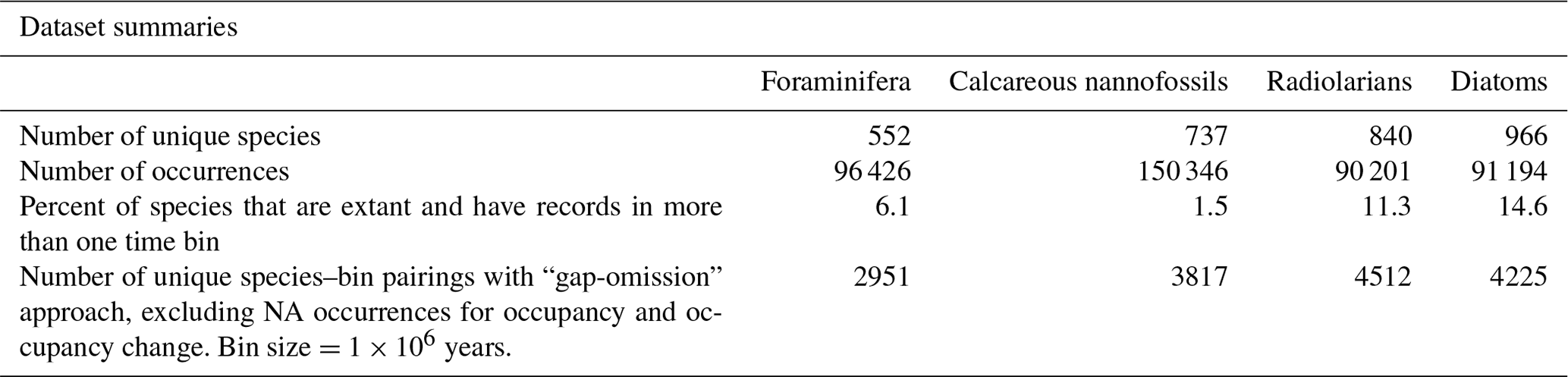
The NSB database includes the estimated age and the modern and estimated paleo-coordinates (longitude and latitude) of each fossil occurrence calculated internally based on the plate tectonic reconstruction by Boyden et al. (2011; Fig. S1 in the Supplement). Each dataset (foraminifera, calcareous nannofossils, radiolarians, diatoms) was cleaned to remove any occurrences that were missing age, paleo-coordinate, and/or relevant taxonomic information. The counts of unique species and the number of occurrence records in each dataset (post-cleaning) are provided in Table 1. All cleaning and subsequent analyses were carried out in R 4.4.3 (R Core Team, 2022).

Table 1 The number of unique species, the number of total occurrence records, the proportion of species that are both extant and occur in more than one bin, and the number of species–bin pairings (post-cleaning).

We assigned occurrences from each dataset to time bins of either 0.1, 0.2, 0.5, or 1.0×10⁶ years, noting that 0.1×10⁶ years is currently the lower limit for global correlation. For each time bin size, the first bin stretched from the present (0 Ma) to either 0.1, 0.2, 0.5, or 1.0×10⁶ years into the past. Each subsequent bin encompassed the following increment stretching progressively further into the past.

We assessed stratigraphic ranges as defined by the oldest and youngest fossil occurrences. Due to reworking and other processes, the documented raw ranges may not reflect the true durations of species. Therefore, we also applied the recommended “Pacman profiling” (Lazarus et al., 2012), a stratigraphic outlier correction, to reduce the impact of outliers and reworking on the data. The degree of Pacman trimming on the NSB data was determined via a calibration process that used speciation and extinction ages of a given subset of each taxonomic group. Based on this subset, the degree of trimming necessary to restore the “true” temporal ranges of species could be estimated. Calibration ages were sourced from the Triton database (Fenton et al., 2021) for foraminifera, Nigrini et al. (2006; obtained from Lazarus et al., 2012) for radiolarians, the “Barron Diatom Catalog” (Lazarus et al., 2014) for diatoms, and a custom species list constructed from Mikrotax (https://www.mikrotax.org, last access: 8 September 2023; Huber et al., 2016) for calcareous nannofossils. Potential trim values ranging from 0 % to 16 % of the raw ranges, at 1 % intervals, were analyzed. Pacman calibration was carried out on datasets after they had been trimmed to the last 66×10⁶ years. Trim values were selected such that they minimized the average absolute difference between the actual and the represented speciation or extinction ages of the species present in the calibration set. The best-performing trim values were implemented in this study, although the key results presented here do not change in the absence of Pacman profiling. Those trim values were as follows: foraminifera (top: 15 %; bottom 3 %), calcareous nannofossils (top: 15 %; bottom: 5 %), diatoms (top: 11 %; bottom: 4 %), radiolarians (top: 10 %; bottom: 7 %). Per capita extinction rates were calculated using the formula from Foote (1999), without normalizing for interval length.

2.2 Analysis of completeness

In order to quantify the degree to which sampling completeness affected downstream analyses, we employed two separate completeness metrics: the three-timer completeness metric (Alroy, 2008) and the simple completeness metric (SCM; Benton, 1985). The three-timer completeness metric is the ratio of “three-timer” taxa (those which occur in bin i−1, bin i, and bin i+1) to all taxa which occur in both bin i−1 and bin i+1 (irrespective of their presence in bin i, “part-timer” taxa). The three-timer metric was calculated from the three-timer and part-timer counts returned by the “divDyn” R extension package (Kocsis et al., 2019; version 0.8.3). The simple completeness metric is the ratio of time bins with confirmed taxon occurrences to the inferred (by recorded observations before and after a focal time interval) number of time bins occupied by that taxon.

2.3 Calculating occupancy

For each dataset, paleo-coordinates of samples were assigned to equal-area geographic cells using the R package “icosa” (Kocsis, 2020; version 0.11.1) for the calculation of proportional grid occupancy. Proportional grid occupancy is a recognized metric for assessing geographic range in the fossil record, where contemporaneous sampling is impossible and incomplete preservation is common (Foote et al., 2007; Darroch et al., 2022). Several cell sizes were analyzed ranging in edge length between 3.33 and 2°. There was little variation in results within this range, so the highest resolution (4002 cells with 2° edge length, mean area of 1.3×10⁵ km²) was selected for this study. The present-day distribution of samples can be seen in Fig. S1.

As counts of occupied cells tend to be biased by sampling (Kiessling, 2005), we calculated the proportional occupancy of each species in every time bin. Proportional occupancy is the number of geographic cells occupied by the species divided by the total number of sampled cells in a given time bin. For simplicity, we refer to what is actually proportional occupancy as occupancy from here forward. Furthermore, the number of unique Longhurst (2007) biogeographic planktonic provinces that were occupied by each species in each time bin was calculated, and the Pearson correlation of this value with the raw number of occupied geographic cells was calculated. Autocorrelation was accounted for by differencing temporally consecutive values prior to calculating correlation values.

2.4 Change in occupancy

In addition to standing occupancy, the change in occupancy between consecutive time bins was calculated by taking the natural log of the ratio of occupancy in time bin i to occupancy in time bin i−1. The log transformation serves to standardize the magnitude of change and produces positive values for increases in occupancy (range expansions) and negative values for decreases in occupancy (range contractions). The correlation of the first differences between occupancy and occupancy change was computed to determine if the data were affected by multicollinearity.

Initially, instances where occupancy values in bin i or i−1 were 0 (no occurrences) were coded as missing data for occupancy change and removed from the final dataset. While removing these records prevents the inclusion of undefined occupancy change values in the final dataset, it greatly reduces the number of occurrences for a given taxon, especially for species whose sampling is fragmentary. This effect is magnified by the fact that, for each time bin with zero occurrences of a given taxon (a “gap” in that taxon's fossil record), two data points are removed from the final dataset for that taxon. This overall loss of data becomes more pronounced with smaller bin sizes.

To combat this effect, we employed a “gap-omission” approach, whereby the change in occupancy was calculated based on the previous occurrence of the taxon (regardless of when that was) rather than the previous time bin per se. Thus, i and i−1 do not necessarily correspond to sequential time bins in this approach but rather to consecutive positive sampling intervals for each given taxon. With this approach, consecutive taxon occurrences are included even when separated by “gaps”, thus retaining more data to the final dataset. Although both approaches yield the same basic results (see Tables S1 and S2 in the Supplement), we used the “gap-omission” approach for the sake of retaining a larger dataset.

2.5 Binomial logistic modeling

For every species, a record of each time bin in which that species occurred was included in the final dataset as a single row. Each unique species–bin pairing (row) is characterized with the occupancy and a binary extinction indicator in the focal time bin and the change in occupancy from the previous time bin. An extinction indicator value of 1 was assigned if an occurrence was the last time bin in which a species occurred for the entire dataset (the species went extinct or permanently disappeared from the fossil record during this interval). An extinction value of 0 was assigned for all other occurrence records (the species did not go extinct during this interval). Species that are still extant, or those which only went extinct during the most recent time bin (which spans to the present), would by default be assigned an extinction value of 1 in the most recent time bin. To avoid this edge effect, all occurrences from the most recent time bin were removed prior to model fitting.

Binomial logistic models were constructed to examine the dependency of extinction on occupancy and occupancy change. Both variables were examined with respect to the per-interval probability of extinction. The saturated generalized linear model structure of “glm(extinction ∼ occupancy * occupancy_change, family = binomial(link = `logit'))” was used. The stepAIC() function in the R package “MASS” (Ripley et al., 2013; version 7.3) was used to select the best-fitting model containing some combination of these variables and their interaction term.

2.6 Model performance and predictor importance

We calculated the adjusted amount of deviance (D² of Guisan and Zimmermann, 2000) accounted for by each computed logistic model. Deviance in a generalized linear model is analogous to variance of ordinary linear regression. In each of the 16 datasets (four groups with four time resolutions each), the Lindeman, Merenda, and Gold (LMG; 1980) indices of correlated input relative importance (henceforth referred to as “relative importance”) were calculated for the occupancy and occupancy change terms with respect to predicting the extinction term. This statistical approach was used to represent the explanatory power of each model term with respect to another, an insight that is not directly apparent with simple model coefficients.

2.7 Extinction probabilities of extant species

The World Register of Marine Species (https://www.marinespecies.org/, last access: 25 September 2023), with the assistance of the R package “taxize” (Chamberlain and Szocs, 2013; version 0.9.100), was used to identify extant species. These data on extant taxa were downloaded on 25 September 2023.

In order to predict the extinction probabilities of extant species, the datasets were reanalyzed and re-fitted to models using only the extinct species. Although this technique reduced the overall amount of data used to fit the model, it allowed the prediction of extinction probabilities of extant species without circularity. Other than removing extant species, all other processes were carried out in the same way as described above.

After selecting the best model for each plankton group, that model was used to predict the extinction probability of extant species. Using the fitted models along with the occupancy and occupancy change values for each extant species in the present bin (that which ends at the present, 0 Ma), a probability of the binary response variable occurring as a 1 (extinction) can be calculated. This represents the probability that the species will not appear again during the next time bin of the same length (that which begins at the present, 0 Ma) or in other future time bins. Extinction predictions were made on extant species subsets without upper Pacman trimming, and the average probability of extinction for all extant species was calculated in each dataset.

2.8 Robustness testing

Further analyses tested the robustness of our results, specifically for the proportional occupancy's utility as a metric of geographic range. The same analyses at a bin size of 1×10⁶ years were carried out using latitudinal range and change in latitudinal range instead of proportional occupancy and its change. Additionally, the same analyses were carried out using proportional occupancy of Longhurst (2007) provinces and the change in proportional occupancy of Longhurst provinces for data sorted into 1×10⁶-year bins. Mixed-effect models, in which each taxon was regarded as a random effect, were also constructed to check if species identity substantially impacted the basic model results.

Although it contains only records of planktonic foraminifers (many of which were sourced from the NSB), the Triton database includes information on the original purpose of each study from which records were sourced, along with the age of speciation and extinction for each species. With this additional information, the Triton dataset can be used to confirm the suitability of methods used with the Neptune dataset with a different collection of fossil occurrences. Given that some studies may not record every present taxon if it is not a zonal marker or thought to be particularly informative, the Triton dataset was subset to include only studies whose purpose was noted as “community analysis” (Fenton et al., 2021). Because studies whose purpose was to analyze community structure would likely document all present species, by using this subset, studies that potentially excluded some species were removed from the final dataset. Additionally, each included species history was subset to exclude any occurrences that occurred before or after the speciation and extinction ages noted in the Triton dataset, respectively, reducing the potential impact of reworked fossils in the analysis. Because each species in Triton was trimmed in this manner, these data did not undergo Pacman profiling as the NSB data did. After these additional data-cleaning actions were taken, the Triton dataset had 197 832 usable occurrence records and was analyzed in the same way as the NSB data.

3 Results

The utilized datasets show all four groups with elevated extinction rates coming out of the end-Cretaceous mass extinction and returning to relative stasis approximately 5–15 Ma after the event (Fig. 1). All groups underwent decreases in diversity, corresponding with the Paleocene–Eocene Thermal Maximum (PETM; Fig. S2). Radiolarians and diatoms show spikes in extinction (>0.4) during the Eocene, including at the Eocene–Oligocene transition and at approximately 44 and 41 Ma. The extinction rates (Fig. 1) and diversity patterns (Fig. S2) of each plankton group match those of previous analyses of Neptune data (Jamson et al., 2022), and various biotic events in the Cenozoic, including the Eocene–Oligocene and the Oligocene–Miocene transitions, can be detected.

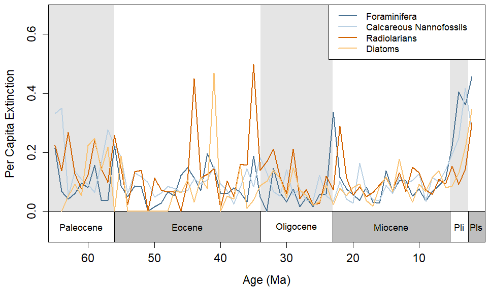
Figure 1 Per capita extinction rates calculated using the formula in Foote (1999) for each of the four taxonomic groups during the Cenozoic, calculated with 1×10⁶-year bins. The timescale of Gradstein et al. (2012) was used here to match age assignments in the NSB.

Occupancy is statistically significant (i.e., statistically non-zero, p=0.05) in all of the analyzed combinations of taxonomic group and bin size. Occupancy change is significant in all models except for calcareous nannofossils with a bin size of 0.2 Ma (Table 2). The term for the interaction between occupancy and occupancy change is significant in all but three models: foraminifera with bin size of 0.2 Ma, foraminifera with a bin size of 0.5 Ma, and diatoms with a bin size of 1.0 Ma (Table 2).

Table 2 Relative importance values shown with standard error for the occupancy, occupancy change, and interaction term for each group at each bin size. The D² values for each model are also reported. Darker blue corresponds to higher values. F = foraminifera, N = calcareous nannofossils, R = radiolarians, D = diatoms.

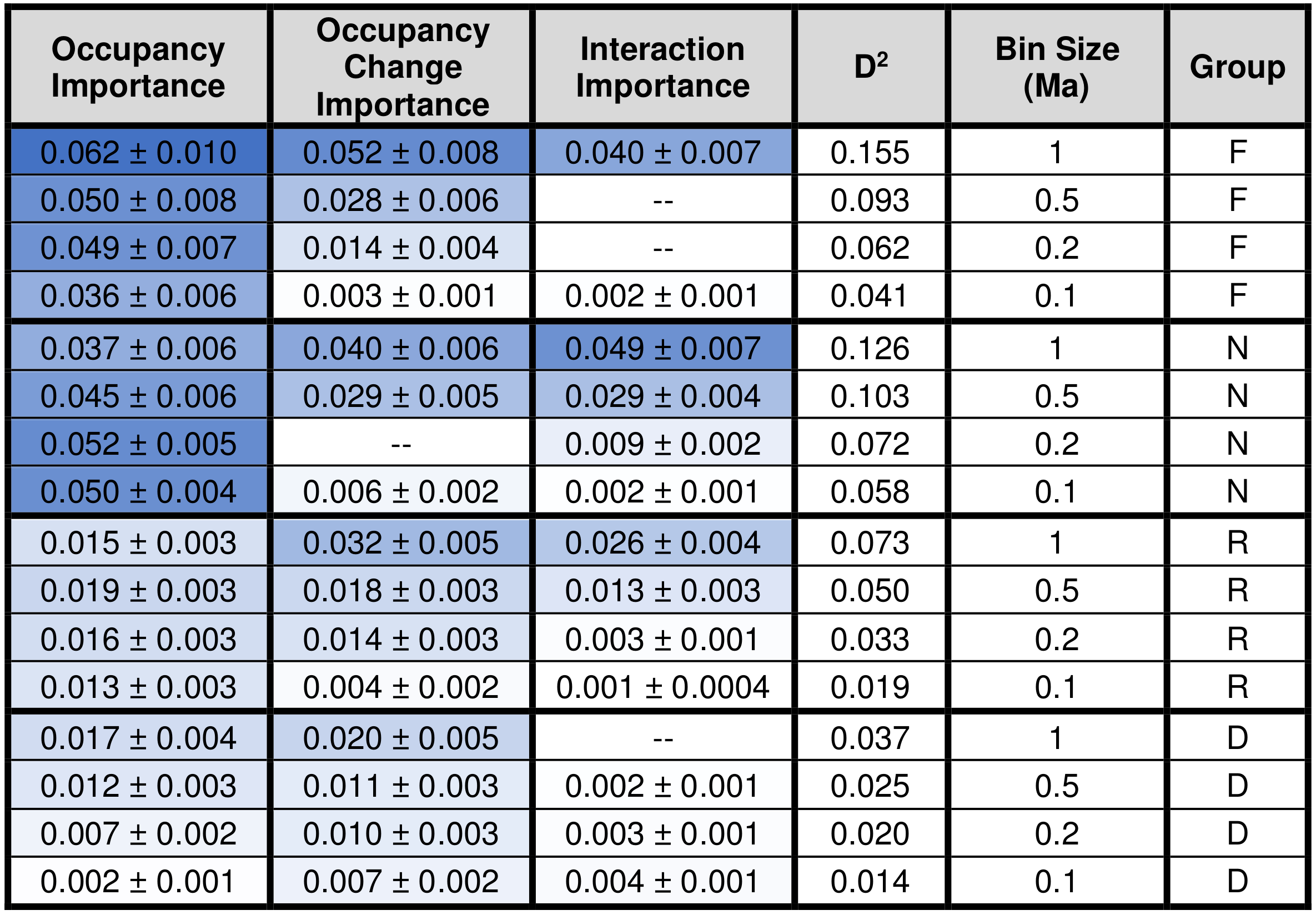
The signs of the occupancy and the occupancy change coefficients are always negative (Table 3), meaning that smaller instantaneous geographic range sizes and more negative changes in geographic range size both correspond to larger extinction probabilities (Fig. 2). The D² values of each analyzed model combination set are shown in Table 2. The maximum D² for any model is 0.155, occurring for the saturated foraminifera model at a bin size of 1.0 Ma. The relative importance of the occupancy change term averages 0.019, or about 41 % of the total explanatory power shared by occupancy and occupancy change, with higher values being achieved with larger bin sizes.

Table 3 Model coefficients for the occupancy, occupancy change, and interaction term for each group and bin size. Darker blue corresponds to more positive values, and darker red corresponds to more negative values. F = foraminifera, N = calcareous nannofossils, R = radiolarians, D = diatoms.

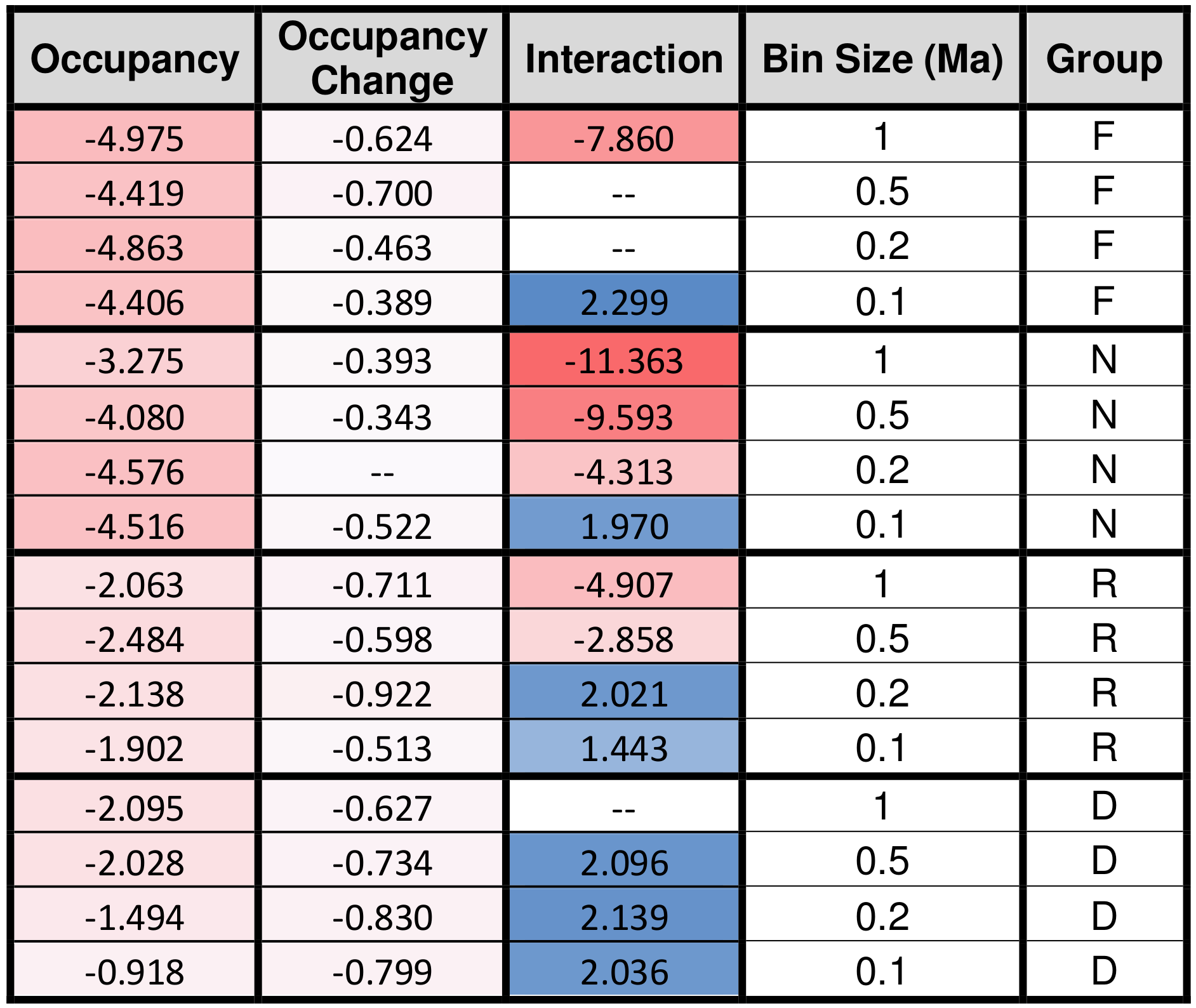
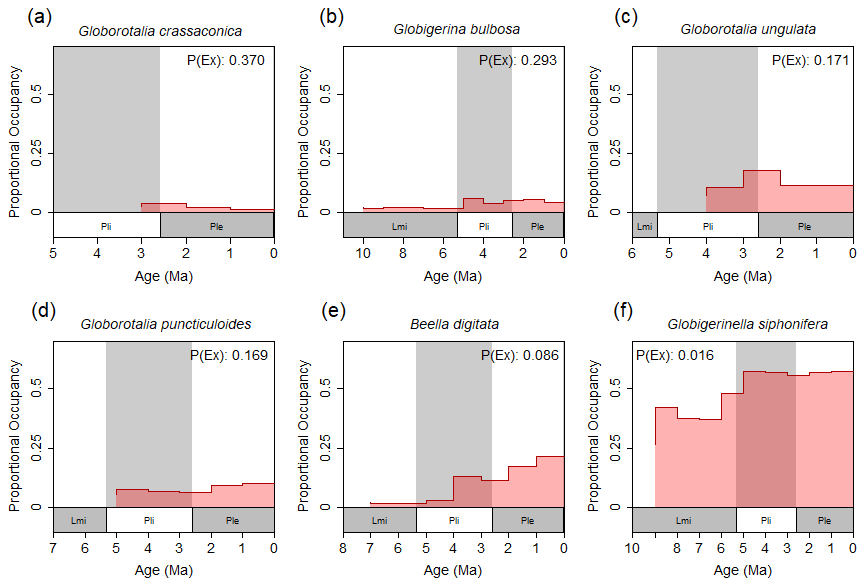
Figure 2 A selection of proportional occupancy through time plots for six species of foraminifers sourced from the NSB with 1×10⁶-year bin size. In each panel, the current extinction probability of that species – predicted for the next 1×10⁶ years using that species' historical geospatial records – is shown. Panels (a) through (f) are ordered according to decreasing current extinction probability. Note the association of relatively small standing occupancy values and relatively large occupancy decreases with increased probability of extinction. “Lmi” = Late Miocene, “Pli” = Pliocene, “Ple” = Pleistocene.

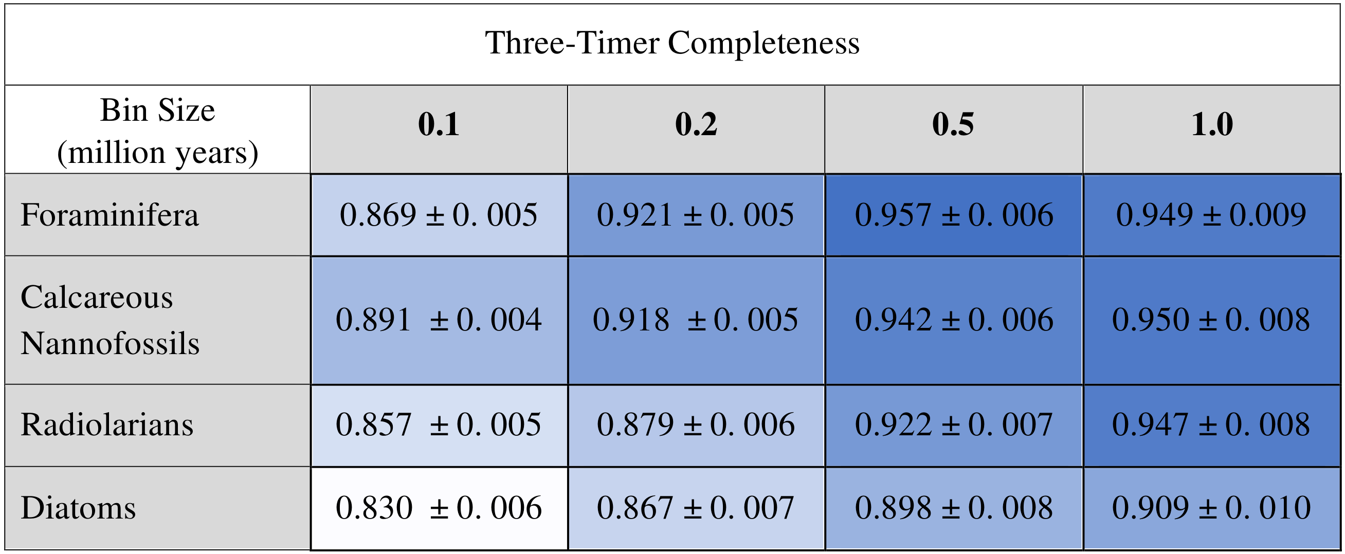
D² values and relative importance values of the occupancy change term increase systematically with bin size, and calcareous organisms tend to have higher values than siliceous organisms for both metrics (Table 2), indicating better overall explanatory power in calcareous organisms. The maximum relative importance value of occupancy is 0.062, and the maximum relative importance value of occupancy change is 0.052, both of which were reported for the foraminifera dataset with a time bin of 1.0 Ma (the D² of this particular saturated model is 0.155). Not surprisingly, sampling completeness increases with larger temporal grain. Foraminifera and calcareous nannofossils have consistently higher three-timer sampling completeness than the siliceous groups across all bin sizes (Table 4; see Table S3 for SCM completeness).

Table 4 Three-timer completeness scores (Alroy, 2008) calculated for each full dataset at each of the four examined bin sizes. Shown with 95 % confidence intervals.

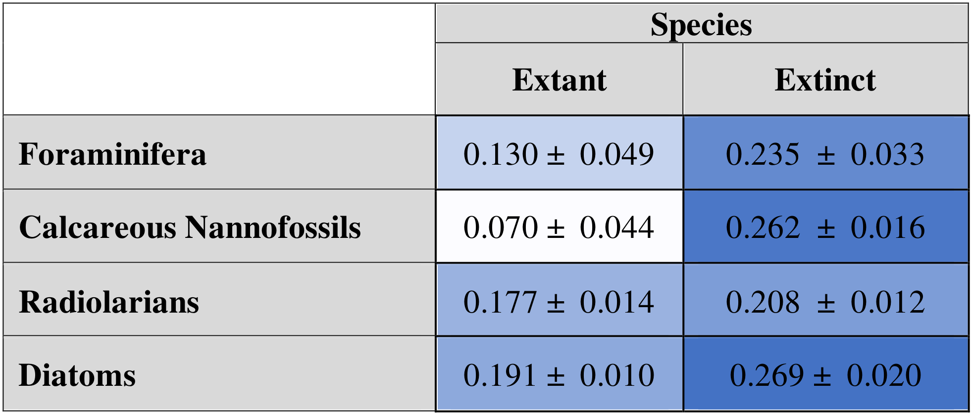
When fit to extinct-only data subsets, AIC-selected models still retain both the occupancy and the occupancy change term for all groups at all bin sizes. Extant diatoms show a significantly higher probability of extinction than the two calcareous groups, and extinct radiolarians have a significantly lower probability of extinction than calcareous nannofossils and diatoms (Table 5).

Table 5 Mean of all extant-organism extinction probabilities (left) and extinct-organism extinction probabilities (right) produced for each dataset. Means are shown with 95 % confidence interval.

The raw number of cells occupied by each species during each time bin shows a strong positive correlation with the number of occupied Longhurst provinces for each taxonomic group at each bin size, even when autocorrelation is removed (Table S4). The same analyses conducted on proportional occupancy of Longhurst provinces and on the change in proportional occupancy of Longhurst provinces, as well as on the latitudinal range of species and the change in latitudinal range of species, yield best-fit models that retain both variables and their interaction term (Tables S5 and S6). When the logistic modeling is applied to the Triton data, both the occupancy and the occupancy change terms are retained across the three largest bin sizes (Table S9). The maximum D² value of 0.072 is achieved with a bin size of 1.0 Ma, and the LMG values of occupancy and occupancy change are 0.050 and 0.016, respectively. Tests for multicollinearity show only minor correlation (mean=0.23, maximum=0.32) between the examined variables (Table S7). Although several datasets failed to reach convergence, the mixed-effect models show similar results to those reported as part of the main analysis (Table S8).

4 Discussion

4.1 Geographic range as a driver of microplankton diversity

While absolute geographic range size is an informative predictor of extinction risk, various other factors relating to geographic range also play an important role in global biodiversity patterns. Powell and Glazier (2017) found that, in the same four groups of microplankton analyzed in this study, latitudinal diversity gradients are produced by asymmetric shifts in geographic range, rather than variations in diversification rate with respect to latitude. On the contrary, Raja and Kiessling (2021) found that the extratropics had higher average origination rates than the tropics. Supporting the finding of Powell and Glazier (2017) that asymmetric shifts in geographic range are key drivers of latitudinal diversity gradients, Raja and Kiessling (2021) showed that dispersal was more likely to occur from the extratropics towards the tropics. Both studies suggest that latitudinal diversity gradients, and thus the geographic distribution of a species, are closely linked to paleoclimate regimes. Indeed, changes in global circulation patterns, water column stratification, and temperature are all among the major influences on global plankton diversity (Lowery et al., 2020)

Although the ranges of marine microplankton have been known to shift in response to climate (Ying et al., 2024; Chaabane et al., 2024), this is not always the case, as species ranges sometimes fail to keep up with shifting temperature zones (Trubovitz et al., 2020). Trubovitz et al. (2023) found that radiolarian abundance is not a significant predictor of extinction risk and that external drivers (such as climate) are more likely to predict extinctions. Thus, while some species do migrate in response to climate change, larger geographic ranges may provide a geographic cushion to species that do not: as local temperatures change, more widespread species undergo a more drawn-out series of local extirpations before global extinction occurs. This agrees with the well-established phenomenon, which we also report here, that larger instantaneous geographic occupancy reduces a species' risk of extinction (Foote et al., 2016, 2007; McKinney, 1997; Payne and Finnegan, 2007; Purvis et al., 2000; Staude et al., 2020).

Additionally, the trajectory of a species' geographic range through time might indirectly reflect shifts in regional or global climate. As paleoclimate zones shift, geographic cells may become inhospitable to a species, and the species may undergo extirpation in that geographic cell. A more rapid change in a species' occupancy through time may reflect a more rapid change in paleoclimate and hospitable regions of Earth. Continued reduction in occupancy over time can thus provide insight into the effects of long-term climatic, geographic, or biological trends on the extinction probability of marine microplankton.

4.2 History of occupancy/legacy effects

The trajectory of various ecological variables through time has been shown to impact the current and future direction of species diversity trends. These legacies may include past climatic events or geographic range shifts influencing modern distributions or extinctions of species (Svenning et al., 2015). The interaction of historic information with current information can provide insight about ecological processes that neither historic nor current information could provide on its own.

The historic trajectory of climate change impacts the probability of extinction occurring with a short-term change in climate. A warming event occurring after a long-term warming trend leads to greater extinction rates (Mathes et al., 2021) than a warming event occurring after a long-term cooling trend. Understanding the historical conditions leading up to a study period of interest may thus be essential to understanding the key drivers as to what goes extinct versus what survives.

Although the effect of climate and geographic range legacies on instantaneous geographic range is well studied (Svenning et al., 2015), the effect of geographic range legacies on instantaneous extinction probability has not received as much attention. Of course, populations of species cannot “look” backwards but are instead influenced by the current conditions present in an environment. The predictive capability of the occupancy change term may thus be an indicator of continued unfavorable conditions (perhaps spanning millions of years) acting on a population at a given time. Kiessling and Kocsis (2016) found that the legacy of geographic range (represented as its change to the present from the previous bin) is an informative predictor for extinction risk in marine macroinvertebrates. Our results build upon those of Kiessling and Kocsis (2016), demonstrating that these findings hold true for marine microplankton and that temporal scale (bin size) is a key variable in detecting the importance of geographic legacy effects.

4.3 Scale dependency of extinction drivers

Although previous studies have analyzed various drivers of extinction through geologic time, relatively little research has gone into understanding the scale dependency of these extinction drivers. Scale dependency in extinction studies manifests in various variables, such as area (Fagan et al., 2005; Guardiola et al., 2013) or taxon age (Henao Diaz et al., 2019). Analyzing data at different temporal scales is also imperative to detect true ecological signals (Hewitt et al., 2010). We find that, as temporal resolution decreases (bin size increases), the relative importance of both the occupancy and occupancy change variables increases (Table 2).

This could result from there being more records in a single temporal bin as bin size increases, thus increasing statistical power. With larger bin sizes, it is easier to detect biological signals that may otherwise be lost in the noise of fragmentary data. We show here that the seemingly arbitrary selection of temporal bin size can have major impacts on conclusions drawn about microplankton diversification and that coarser resolutions may more reliably indicate actual macroevolutionary trends.

4.4 Calcareous vs. siliceous microfossils

In general, the explanatory power of each of the model terms is smaller in the siliceous groups than in the calcareous groups. Although occupancy and occupancy change were found to be informative across all groups, the signals are weaker in diatoms and radiolarians (Tables 2 and 3). This discrepancy likely results from minor variations in sampling, as evidenced by lower three-timer completeness values for the two siliceous groups. The difference may also be a result of variable taphonomic pathways between the calcareous and siliceous organisms (Boltovskoy, 1994). Nonetheless, both occupancy and occupancy change are important predictors of extinction regardless of the group, and these findings further underscore the importance of accounting for sampling when analyzing paleontological data.

4.5 Robustness testing

There is a strong correlation between the number of occupied Longhurst provinces and the number of individual occupied geographic cells for each species–bin pairing. This demonstrates that, although the locations of the various drilling expeditions that sourced much of the data in the Neptune database are not entirely random, when taken together, they still account for a diverse spread of planktonic biogeographic regions around the globe. This supports the idea that the collection of data contained in the Neptune database is comprehensive enough to study large-scale biogeographic trends. Additionally, AIC-selected models contained both the occupancy and occupancy change terms even when geographic range was measured as latitudinal expanse or as a proportion of occupied Longhurst provinces (Tables S5 and S6). This suggests that the significance of proportional occupancy change in predicting extinction is not merely an artifact of data processing.

The AIC-selected model for each bin size in the Triton dataset always retains both occupancy and occupancy change as significant except with a bin size of 0.1 Ma (Table S9). Although the Triton dataset has substantially more occurrence records after preprocessing, it has consistently lower diversity compared to the other taxonomic groups from the NSB (Fig. S2). This could indicate a greater propensity for “lumping” in the Triton dataset than in the NSB, which in turn could change how spatiotemporal signals manifest. The similar results obtained from the Triton dataset further confirm the suitability of these methods with an alternative dataset and reaffirm the importance of occupancy and occupancy change when modeling extinction.

Taken together, our findings suggest that the change in geographic occupancy is an important metric for predicting extinction across marine life. Kiessling and Kocsis (2016) looked exclusively at skeletal macroinvertebrates, whereas we analyze several protist lineages of marine plankton. The broad taxonomic scope of these findings emphasizes the fundamental importance of the trajectory in geographic range as a biological metric, which can be a key aspect of taxon dynamics through time. Although the explanatory power of the model may seem low (up to 15.5 %), it is an important factor given the many other variables that influence extinction risk (McKinney, 1997)

4.6 Future perspectives

Although modern studies can track geographic occupancy change over the course of decades (if there is a history of consistent data collection), estimates of marine species durations average between 5–10×10⁶ years (Foote and Raup, 1996; Raup, 1991), much longer than human-collected records can encompass. To fully understand the change in occupancy through a species' duration, records extending beyond those which could have been manually recorded by conservation biologists are needed. Although some modern conservation practitioners have been hesitant to fully embrace long-term paleontological data, this study provides yet another argument for the incorporation of historical perspectives and fossil evidence in conservation efforts (Dietl et al., 2019; Kiessling et al., 2019; Smith et al., 2018).

While, for simplicity's sake, this study only looked at the interaction of occupancy and the first degree of occupancy change (bin number i to i−1), future iterations could incorporate entire occupancy histories into model fitting using even more advanced techniques. This may help the model overcome variations in sampling intensity or localized paleoenvironmental events and let the models provide information not only on decline but also on continued decline – another hallmark of increased extinction risk.

5 Conclusion

In providing evidence that the geological history of species distributions plays a significant role in species extinction risk, our study demonstrates the importance of paleontological data for assessing modern species extinction risk. These findings provide empirical support for the connection between continued range reduction and ultimate global extinction in marine microplankton. We also demonstrate the importance of temporal grain in detecting biological signal in fragmentary fossil data.