Does increased spatial replication above heterogeneous agroforestry improve the representativeness of eddy covariance measurements?

Spatial heterogeneity in terrestrial ecosystems compromises the accuracy of eddy covariance measurements. Examples of heterogeneous ecosystems are temperate agroforestry systems, which have been poorly studied by eddy covariance. Agroforestry systems have been getting increasing attention due to their potential environmental benefits, e.g. a higher carbon sequestration, improved microclimate and erosion reduction compared to open-cropland agricultural systems. Lower-cost eddy covariance setups might offer an opportunity to better capture spatial heterogeneity by allowing for more spatial replicates of flux towers. The aim of this study was to quantify the spatial variability of carbon dioxide (FC), latent heat (LE) and sensible heat (H) fluxes above a heterogeneous agroforestry system in northern Germany using a distributed network of three lower-cost eddy covariance setups across the agroforestry system. Fluxes from the three towers in the agroforestry were further compared to fluxes from an adjacent open-cropland site. The campaign took place from March 2023 until September 2024. The results indicated that the spatial variability of fluxes was largest for FC, attributed to the effect of different crops (rapeseed, corn and barley) within the flux footprints contributing to the measured fluxes. Differences between fluxes across towers were enhanced after harvest events. However, the temporal variability due to the seasonality and diurnal cycles during the campaign was larger than the spatial variability across the three towers. When comparing fluxes between the agroforestry and the open-cropland systems, weekly sums of carbon and evapotranspiration fluxes followed similar seasonality, with peak values of −50 g C m⁻² week⁻¹ and 40 mm week⁻¹ during the growing season, respectively. The variation of the magnitude depended on the phenology of the different crops. The effect size, which is an indicator of the representativeness of the fluxes across the distributed network of three eddy covariance towers compared to only one, showed, in conjunction with the other results, that the spatial heterogeneity across the agroforestry was better captured by the network of three stations. This supports previous findings that spatial heterogeneity should be taken into account in eddy covariance studies and that lower-cost setups may offer the opportunity to bridge this gap and improve the accuracy of eddy covariance measurements above heterogeneous ecosystems.

1 Introduction

The eddy covariance (EC) technique is the central approach to measuring the exchange of energy, trace gases and momentum between terrestrial ecosystems and the atmosphere (Baldocchi, 2014). The EC technique was established as a standard method within the scientific community when rapid-response instruments, capable of measuring wind speed, temperature and gas concentrations over the major frequency ranges of the turbulent energy spectrum, became commercially available (Aubinet et al., 2012; Wohlfahrt et al., 2009). These instruments provided the capability to measure the exchange of energy and matter between the land surface and the atmosphere, driven by eddies of diverse sizes and frequencies (Kaimal and Finnigan, 1994).

At a majority of flux sites, a single EC station is installed (Hill et al., 2017), and measurements are made based on the ergodic hypothesis. The ergodic hypothesis states that covariances (fluxes) calculated over the time domain are equivalent to covariances calculated over the spatial domain (Higgins et al., 2013). The measured turbulent fluxes and carbon and water balances, when integrated over a defined time interval, are representative of the tower footprint area corresponding to the averaging interval (Vesala et al., 2008). This is true for homogeneous sites where the spatial representativeness of fluxes within the ecosystem of interest is guaranteed with a high degree of confidence (Hurlbert, 1984). However, these conditions of homogeneity are often not met in many ecologically and socioeconomically interesting sites, such as mixed forests, wetlands, urban forest interfaces or small-scale farmlands (Finnigan et al., 2003; Hill et al., 2017).

Agroforestry (AF) systems are an example of heterogeneous agroecosystems. They combine trees and crops on the same agricultural land in order to benefit from the presence of trees on the land (Veldkamp et al., 2023; Kay et al., 2019). These systems offer several benefits, including the potential to prevent wind erosion over crops (van Ramshorst et al., 2022; Böhm et al., 2014), improve soil fertility (Kanzler et al., 2021) or reduce water loss through evaporation in crops (Kanzler et al., 2019). Short-rotation alley-cropping systems, a type of agroforestry, represent an alternative land use practice with the potential to increase carbon sequestration and improve water use efficiency (WUE) in comparison to conventional open-cropland (OC) agriculture (Markwitz et al., 2020; Veldkamp et al., 2023). These AF systems consist of alternating rows of trees and crops. The trees employed in these systems are typically fast-growing species, such as poplar (Populus) or willow (Salix), and are harvested in cycles of 5–6 years for biomass production. Crops are cultivated in an annual rotation.

In general, heterogeneity poses a challenge for EC measurements and, in a broader context, for any type of measurement across the atmospheric boundary layer (Bou-Zeid et al., 2020). Heterogeneity in surface properties induces horizontal advection, secondary mesoscale circulations and non-equilibrium turbulence processes, which occur near to and downstream of changes in the surface properties (Bou-Zeid et al., 2020). As shown by previous studies over heterogeneous sites, such as pine forest (Katul et al., 1999; Oren et al., 2006) or managed grassland (Peltola et al., 2015), spatial heterogeneity induced relevant spatial variability in the EC measured fluxes. According to the classification of Bou-Zeid et al. (2020), the heterogeneity of these AF systems can be classified as unstructured heterogeneity (see their Fig. 1) because the site consists of a certain number of interleaved trees and crop strips, but it is small enough that the AF site might be affected by other elements in the surrounding landscape. Upon changes in surface properties (like roughness or moisture), the mean wind field and the turbulence adjust to the new surface, with more complex effects on the flow when multiple changes in the surface properties co-occur, as is the case with the AF (Bou-Zeid et al., 2020).

The location of the EC station within a land use system has been demonstrated to potentially introduce a bias into the measured fluxes (Chen et al., 2011), indicating that a single EC station may not be sufficient to properly account for the spatial variability of fluxes induced by landscape heterogeneity (Katul et al., 1999). The high cost and labour intensity of deploying an EC station are the main reasons for the lack of spatial replicates of EC measurements in many studies (Hill et al., 2017). The infrared gas analyser (IRGA), the crucial component to measure trace gases, typically accounts for a large proportion of the total installation costs associated with an EC station. Lower-cost EC (LC-EC) setups represent a potential solution to the spatial replication problem of EC measurements as several EC stations could be deployed for the cost of a single conventional station. LC-EC employs a more economical infrared gas analyser and a sonic anemometer, though these instruments necessitate more rigorous post-processing corrections. Notably, previous studies have demonstrated that LC-EC setups can yield comparable results to those of conventional EC (CON-EC) setups. Hill et al. (2017) compared a custom-built LC-EC setup for CO₂ and H₂O measurements with a CON-EC, with very good agreement in terms of CO₂ and H₂O fluxes. In addition, a different LC-EC setup for H₂O flux measurements was compared with a conventional setup (Markwitz and Siebicke, 2019), resulting in good agreement in terms of H₂O fluxes. Furthermore, another version of the LC-EC setup deployed in Hill et al. (2017) was extensively validated in the studies of Callejas-Rodelas et al. (2024) and van Ramshorst et al. (2024), with very good agreement in terms of CO₂ fluxes and good agreement in terms of H₂O fluxes.

The LC-EC setups can allow for a higher degree of spatial replication of EC and support conventional EC setups. In addition, they provide a powerful tool for the verification of carbon and water balances in the agricultural and forestry sectors in developing carbon credit markets (Trouwloon et al., 2023) or for an improved water management. However, the increased uncertainty associated with these setups must be taken into account when calculating balances of energy, carbon or other variables and when comparing different land uses. One of the main differences between LC-EC and CON-EC setups is the spectral response of the sensors. The LC-EC setups used in the Callejas-Rodelas et al. (2024), Cunliffe et al. (2022), Hill et al. (2017) and van Ramshorst et al. (2024) studies were characterized by a slower-frequency response in CO₂ and H₂O measurements, which induces a higher spectral attenuation in the high-frequency range of the turbulent energy spectrum, compared to CON-EC. The higher attenuation introduces a greater degree of uncertainty when applying spectral corrections, as observed by Ibrom et al. (2007) and Mammarella et al. (2009), among others.

The impact of landscape heterogeneity within an AF system on turbulence, latent heat flux (LE), sensible heat flux (H) and carbon dioxide flux (FC) remains to be examined. Markwitz and Siebicke (2019) and Markwitz et al. (2020) conducted evapotranspiration (ET) measurements across multiple AF and OC systems in northern Germany; however, their measurements were not replicated within a single site. In contrast, in the study of Cunliffe et al. (2022), a total of eight LC-EC setups were deployed at different locations across a landscape of ecological interest (Cunliffe et al., 2022). The objective of this study was to capture the heterogeneity of FC and ET across a semiarid ecosystem, with low magnitudes of both FC and ET. Replicated EC measurements in heterogeneous agroforestry systems are so far lacking.

In the present study, a network of three LC-EC setups was deployed, analogous to those utilized in the studies of Callejas-Rodelas et al. (2024), Cunliffe et al. (2022) and van Ramshorst et al. (2024), above an AF site, and one additional LC-EC setup was deployed above an adjacent OC site in northern Germany. To the best of our knowledge, this was the first time a distributed network of EC towers has been installed above a temperate agroforestry system. With 1 and a half years of concomitant flux data from the four EC setups, the objective was to quantify the spatial and temporal variability of FC and LE, as well as the statistical effect of the increased spatial replication of EC measurements above a heterogeneous site. According to Hill et al. (2017), it is possible to estimate the sampling variability and total uncertainty for an ecosystem with independent spatial replication of EC measurements. This allows for the estimation of the effect size (see Sect. 2). The present study tested the hypothesis that the increased uncertainty inherent to the use of slower-frequency response sensors in EC measurements can be counteracted by the improvement of the spatial replication of EC, which increases its statistical robustness. The objectives of this study were threefold: (i) to quantify the spatial and temporal variability of turbulent fluxes and parameters above AF; (ii) to calculate the effect size of the experimental site at the daily scale, following Hill et al. (2017); and (iii) to compare the ecological functioning of the AF to that of the OC in terms of FC and ET balances.

2 Methods

2.1 Site description

The measurements were conducted from 1 March 2023 to 19 September 2024 at an agroforestry system located in Wendhausen (Lehre), Lower Saxony, Germany (52.63° N, 10.63° E). The elevation above sea level is 80 m. The field is divided into two distinct systems: an AF system (17.3 ha) in the north and an OC system (8.5 ha) in the south (see Fig. 1). The crops cultivated within both systems kept a similar distribution from west to east. In 2023, rapeseed was cultivated on the western side, barley was cultivated on the eastern side, and corn was cultivated in the centre (Fig. 1a). In 2024, rapeseed was cultivated on the eastern side, barley was cultivated in the centre, and corn was cultivated on the western side (Fig. 1b). The management of the crops was similar at both the AF and OC sites, and crops were fertilized. The mean long-term annual precipitation is 617 mm, and the mean annual air temperature is 9.9 °C for the reference period 1981–2010 at Braunschweig Airport (DWD, 2024). The soil at both the AF and OC sites was classified as a clay Cambisol, with a soil organic carbon (SOC) content of 5.8 kg C m⁻² at the OC site and 6.75 kg C m⁻² at the AF site. Additionally, the soil bulk density was determined to be 1.0 g cm⁻³ at both the AF and OC sites (Veldkamp et al., 2023). Soil characteristics were last measured in 2019.

The harvest of rapeseed, barley and corn in the 2023 campaign season occurred on 13 July, 22 August and 26 September, respectively. The harvest of rapeseed, barley and corn in the campaign of 2024 took place on 15 July, 5 August and 13 September, respectively. In 2024, rapeseed did not grow well, and a mulch cut was carried out; therefore, the eastern part of the field was covered by a combination of grasses, bare soil and mulch. Canopy height was estimated from pictures taken during field visits. The maximum height attained by the crops at the peak of their development stage was around 1.5 m for rapeseed, 2.5 m for corn and 1.3 m for barley. The trees present at the AF system are fast-growing poplar (Populus nigra and Populus maximowiczii) and are typically harvested every 4 to 5 years. The most recent tree harvest occurred in 2019. Trees grew from around 4.0 m till 5.5 m on average across the measurement period.

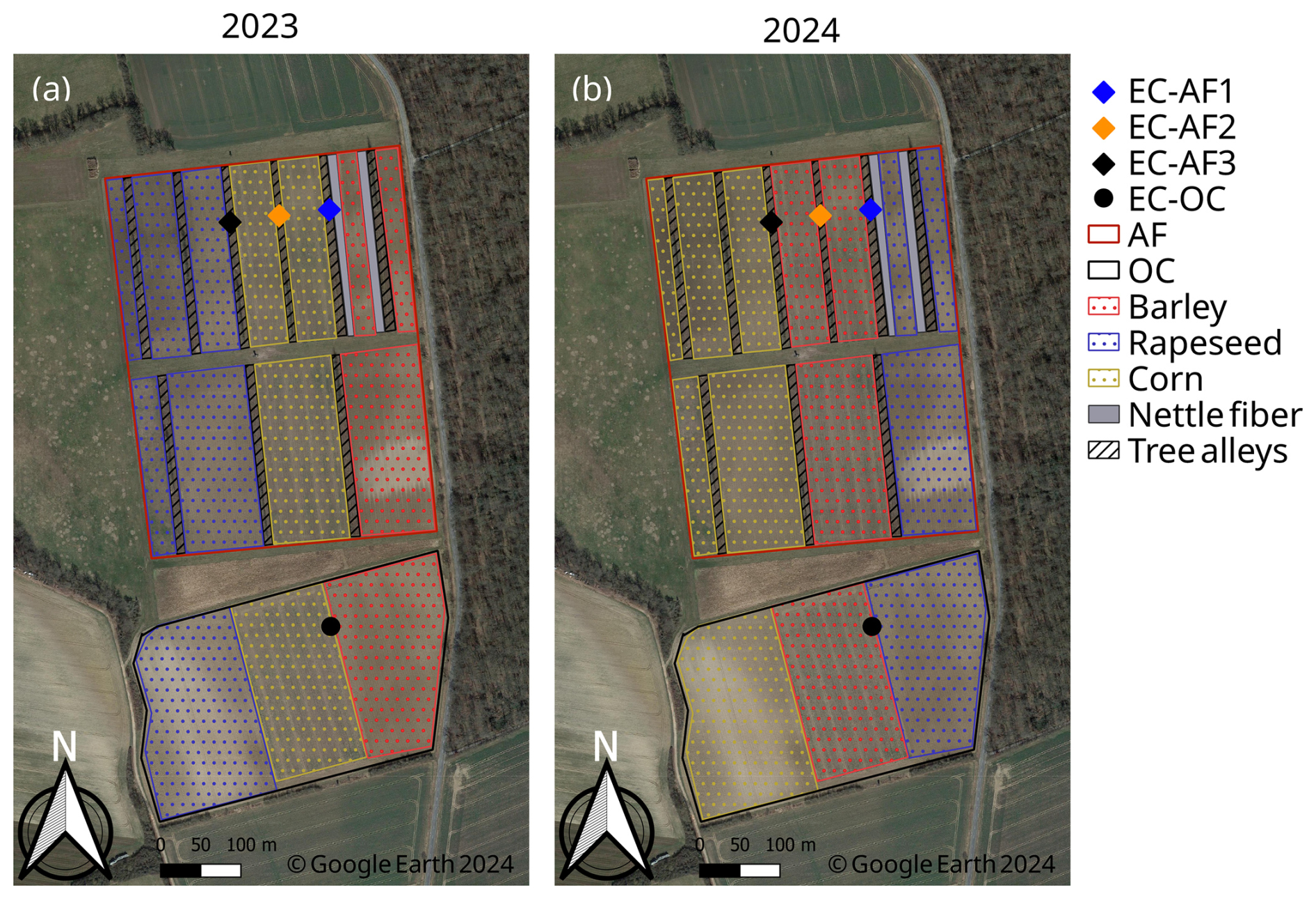
Figure 1 Satellite view and land cover classification of the experimental site for 2023 (a) and 2024 (b), together with the location of the EC stations (blue diamond for EC-AF1, orange diamond for EC-AF2, black diamond for EC-AF3 and black circle for EC-OC). The area bordered by red corresponds to the AF system, and the area bordered by blue corresponds to the OC system. Figure created with QGIS v. 3.22; aerial map by Google Satellite Maps. © Google Earth 2024.

2.2 Experimental setup

Measurements were made at four EC stations, one located at the OC site and three located at the AF site (Fig. 1). The stations are designated as OC, AF1, AF2 and AF3. Each station was equipped with a complete set of meteorological sensors and an LC-EC setup (see Table 1 in Callejas-Rodelas et al., 2024). The measured meteorological variables were air temperature (TA), relative humidity (RH), atmospheric pressure (PA), precipitation (P), global radiation (SW_IN), outgoing shortwave (SW_OUT) and longwave (LW_OUT) radiation, and net radiation (NETRAD). The EC measurement heights were 10 m above ground for AF1, AF2 and AF3 and 3.5 m for OC. Only one photosynthetic active radiation (PPFD_IN) sensor was installed at AF1, and two barometers for atmospheric pressure measurements were installed at AF1 and AF2. All the stations were equipped with two soil heat flux plates to measure soil heat flux (G) at 5 cm depth. Only one soil heat flux plate was installed at AF3. Radiation sensors were placed in a beam facing south at 9.5 m height at AF1, AF2 and AF3 and at 3 m height at OC. TA and RH measurements were taken at 2 m height at all stations. P was measured at 1 (AF1, OC) or 1.5 m (AF2, AF3) height. Meteorological data were recorded on CR1000X data loggers (Campbell Scientific Inc., Logan, UT, USA).

The LC-EC setups consisted of a three-dimensional sonic anemometer for wind measurements (uSonic3-Omni, METEK GmbH, Elmshorn, Germany) and a gas analyser enclosure. The enclosure consisted of an IRGA for CO₂ molar density measurements (GMP343, Vaisala Oyj, Helsinki, Finland) and a RH capacitance cell for RH measurements (HIH-4000, Honeywell International Inc., Charlotte, North Carolina, USA) and was installed at the bottom of the tower. Air was drawn through a 9 m tube at the AF stations and a 2.5 m tube at the OC station. Two temperature sensors were installed, one inside the IRGA measuring cell and one inside the enclosure, along with two pressure sensors, one to measure differential pressure inside the enclosure and another to measure absolute pressure inside the IRGA measuring cell. Measurements from all components were recorded at 2 Hz frequency on a CR6 data logger (Campbell Scientific Inc., Logan, UT, USA). A more detailed description of the setup can be found in Callejas-Rodelas et al. (2024).

The GMP343 sensors were calibrated in February 2023 and February 2024. Frequent inspections were performed to clean the tubing, replace filters, measure flow rate and clean the lens of the GMP343. The nominal flow rate was 5.0 L min⁻¹ at all AF stations, with some drops due to filter clogging.

During the study period, there were generally large percentages of missing data. Missing data were either short gaps (a few 30 min periods or a few hours) caused by data filtering during the quality control after flux processing (see Sect. 2.3.3) or longer gaps (hours to a few days) due to power outages during the winter, mostly at night, at all stations. Due to other technical problems, there were few larger gaps at some stations, particularly a gap of 3 months from mid-July to early October 2023 at AF3, for FC and LE.

Although generally recommended in EC studies (Aubinet et al., 2012), no storage terms were considered in the calculation of FC and LE because no concentration profiles were installed at the stations.

2.3 Flux computation

2.3.1 Pre-processing

Data processing prior to flux calculation included (i) the calculation of CO₂ dry mole fraction measurements from the CO₂ molar density provided by default by the instrument using some sensor-specific parameters and the observed values of pressure and relative humidity in the measurement system (Callejas-Rodelas et al., 2024) and (ii) the calculation of the H₂O dry mole fraction from relative humidity, temperature and pressure measurements inside the measurement cell using the derivation of Markwitz and Siebicke (2019). More details on the pre-processing steps are given in Callejas-Rodelas et al. (2024) and van Ramshorst et al. (2024).

2.3.2 Flux processing

H, LE, FC and momentum flux were calculated using the EddyUH software (Mammarella et al., 2016) in its MATLAB version (MATLAB®R2023a, The Mathworks, Inc., Natick, MA, USA). Raw data were de-spiked using limits for absolute differences between consecutive values. Detrending was performed by block averaging. Wind coordinates were binned into eight sectors of 45° each and rotated according to the planar fit correction procedure of Wilczak et al. (2001), following the default recommendation by ICOS (Sabbatini et al., 2018). Time lag optimization was performed through cross-covariance maximization, using predefined windows of 2 to 10 s for CO₂ and 2 to 20 s for H₂O (Callejas-Rodelas et al., 2024). Low-frequency losses were corrected following Rannik and Vesala (1999), and high-frequency losses were corrected following Mammarella et al. (2009). The latter is based on determining the time response of CO₂ and H₂O separately, calculated from the measured co-spectra. In the case of CO₂, the time response determined by the experimental method was similar to the nominal time response of 1.36 s calculated in Hill et al. (2017) for the GMP343. This time response was used for all flux calculations for all four of the towers. In the case of H₂O, the time response was estimated by a exponential fit as a function of relative humidity. Data quality was flagged from 1 to 9 following Foken et al. (2005).

2.3.3 Filtering and gap filling

Fluxes were filtered using data with quality flags <7 to avoid periods with poorly developed turbulence (Foken et al., 2005). Outliers were removed using a running median absolute deviation (MAD) filter, based on the approach by Mauder et al. (2013), with a window of 2 weeks. The q parameter in Eq. (1) of the paper by Mauder et al. (2013) was set as 7.5. The MAD filter was iterated three times over each time series. Hard upper and lower limits were applied afterwards to remove additional outliers not detected by the MAD filter. Values outside the ranges from −100 to 700 W m⁻² for H, from −20 to 700 W m⁻² for LE and from −50 to 50 µmol m⁻² s⁻¹ for FC were discarded. Additional hard limits were applied specifically to winter (November to February) and transition periods (March and October) separately. The aim was to avoid outliers that went through the previous filters which might bias the application of the gap-filling algorithms. For LE and H, these limits were 50 W m⁻² during winter and 100 W m⁻² in March and October. For the FC, these limits were (in absolute values) ± 10 µmol m⁻² s⁻¹ during winter and ± 15 µmol m⁻² s⁻¹ in March and October. Finally, a friction velocity (USTAR, m s⁻¹) filter was applied to remove periods with non-existent or weak turbulence. The filter of USTAR was applied using REddyProc (Wutzler et al., 2018), which removed values based on a USTAR threshold calculated as the maximum of the seasonally derived USTAR values. These seasonal values were calculated based on Papale et al. (2006). The average USTAR thresholds for the stations were 0.21, 0.21, 0.18 and 0.16 m s⁻¹ for AF1, AF2, AF3 and OC, respectively.

Before filtering, the total available data accounted for 63.4 % (AF1), 80.0 % (AF2), 76.2 % (AF3) and 61.5 % (OC) for FC and LE and 85.7 % (AF1), 86.0 % (AF2), 83.1 % (AF3) and 75.9 % (OC) for H relative to the duration of the entire measurement campaign. These gaps occurred due to instrumental or power failure. After filtering, the available data accounted for 39.3 % (AF1), 49.2 % (AF2), 35.7 % (AF3) and 33.8 % (OC) for FC; 42.0 % (AF1), 53.6 % (AF2), 36.4 % (AF3) and 38.7 % (OC) for LE; and 61.5 % (AF1), 61.4 % (AF2), 56.7 % (AF3) and 52.8 % (OC) for H.

Meteorological data were gap-filled at the 30 min timescale to provide complete time series of the predictor variables for flux gap-filling. The procedure differed slightly for the different variables of interest. Short gaps of up to 1 h were filled using linear interpolation, except for P. Missing data at the AF1 station, when available at the OC station, were filled using linear regression models with the OC data as predictors and vice versa. Missing data at AF2 and AF3 that were available at AF1 were filled using a similar procedure, with AF1 as the reference. Finally, P, TA, RH, vapour pressure deficit (VPD), SW_IN, wind speed (WS) and wind direction (WD) were filled at the stations using ERA5-Land re-analysis data (Muñoz-Sabater et al., 2021) as predictors, following the approach implemented in Vuichard and Papale (2015). Linearly reduced major axis regression models were derived from the ERA5-Land data and the station data using the library pylr2 in Python. The coefficients (slope and intercept) from the linear models were then used to calculate the missing values. PPFD_IN was filled based on global radiation (SW_IN) by multiplying SW_IN by the average ratio between PPFD_IN and SW_IN for the available periods at the site. P was filled by multiplying the ERA5-Land data by the ratio between the station data and the re-analysis data, as in Vuichard and Papale (2015). Any inaccuracies resulting from this replacement did not introduce additional bias into the gap-filled flux time series because precipitation was not used for gap-filling. A quality flag was developed for the meteorological data: 0 indicates measured data, 1 indicates interpolated data, 2 indicates data filled using a nearby station as a reference, and 3 indicates data filled using ERA5-Land as a reference.

Gaps in the flux time series were filled using a double-step procedure, analogous to the approach applied in Winck et al. (2023). Short gaps were filled using the marginal distribution sampling method (Reichstein et al., 2005) with the online version of the REddyProc package (Wutzler et al., 2018). Short gaps were considered by taking the filled data with quality flags of 0 (original measured data) or 1 (highly reliable filled data). Subsequently, the remaining gaps (flagged with 2 or 3 in REddyProc) were filled using a machine learning (ML) tool based on the Extreme Gradient Boosting (XGBoost) algorithm (Chen and Guestrin, 2016). The code was adapted from Vekuri et al. (2023) to include H, LE and FC. The predictor variables of the model were the previously filled TA, VPD, SW_IN, WS and WD. The inclusion of WD followed the recommendation of Richardson et al. (2006) to account for site heterogeneity as different land covers depending on wind sectors can contribute to flux variability. A quality flag was developed for the flux variables: 0 for measured data, 1 for data filled with REddyProc, and 2 for data filled with XGBoost. There were two very long gaps, one for AF3 during summer 2023 (mid-July until beginning of October) and another for AF1 during winter 2023–2024 (beginning of December 2023 until beginning of March 2024), besides gaps with durations of a few days. Such long gaps would introduce significant uncertainty into any gap-filling method, and so the analysis only considered measured and gap-filled data for gaps not exceeding durations of 2 weeks.

The evaluation of the gap-filled fluxes with XGBoost was performed by splitting the initial dataset into 80 % training data and 20 % test data. The root mean squared error (RMSE) between modelled and measured data, for the test dataset, was taken as the error in the individual 30 min flux value (Table 1).

Table 1 Root mean squared error (RMSE) of modelled and measured data for FC, LE and H for the four stations used in this study.

2.3.4 Footprint calculation

A footprint climatology was calculated for all stations for five different periods considered in the study: (i) growing season 2023, from March to 13 July 2023, with the latter being the harvest date of rapeseed; (ii) harvest period 2023, from 13 July to 22 September 2023, with the latter being the harvest date of corn; (iii) winter 2023–2024, from 22 September 2023 to 1 March 2024; (iv) growing season 2024, from 1 March to 15 July 2024, with the latter being the harvest date of the rapeseed; and (v) harvest period 2024, from 15 July to 19 September 2024. The footprint climatology was calculated using the Python version of the model by Kljun et al. (2015).

The input data for the footprint model included non gap-filled wind data (WS, m s⁻¹; WD, °), roughness length (z₀, m), USTAR, Obukhov length (L, m), the standard deviation of lateral wind speed (V_SIGMA, m s⁻¹), boundary layer height (BLH, obtained from ERA5, Hersbach et al., 2023), measurement height (z_m, m) and displacement height (d_h, m). Daytime and nighttime values were used for the footprint modelling. z₀ and d_h were estimated from the aerodynamic canopy height (h_a, m), which was calculated under near-neutral conditions (stability parameter $\left|\right(z-d)/L|\le \mathrm{0.1}$) using the procedure described by Chu et al. (2018). Complete time series of h_a were estimated by calculating the running mean of h_a for eight different wind sectors of 45° each using a running mean of 100 30 min intervals. This procedure is described in more detail in van Ramshorst et al. (2025). This procedure allowed for a more comprehensive representation of the effects of a varying canopy roughness and is therefore more precise than using a single value to represent the average canopy height for the entire site at each time step. d_h and z₀ were calculated as 0.6 and 0.1 times the aerodynamic canopy height, respectively, following Chu et al. (2018). The mean values of d_h were 3.1 m at the AF site and 0.6 m at the OC site, while the mean values of z₀ were 0.5 at the AF site and 0.1 m at the OC site. A thorough discussion about the footprint model uncertainties can be found in Sect. 4.4.

2.4 Spatial and temporal variability of fluxes and turbulence parameters and effect size

To disentangle the spatial and temporal variability of fluxes and turbulence parameters across the site, the data were classified in two ways. First, the data were aggregated into wind sectors of 45° each, similarly to the sectors used for the planar fit division (see Sect. 2.3), and separated into five time periods as described in the previous paragraph. Second, the data were grouped into 1-week periods throughout the entire measurement campaign without division into wind sectors. For each classification, coefficients of spatial variation (CVs) were calculated, and the variance was partitioned into temporal and spatial components. In this analysis, we used only measured data filtered according to the previously described criteria and not gap-filled data.

The CVs were defined as

$$\begin{array}{}\text{(1)}& {\mathrm{CV}}_x=\stackrel{\mathrm{‾}}{\left[{\displaystyle \frac{<\left[x\right(t)-X(t){]}^{\mathrm{2}}{>}^{\frac{\mathrm{1}}{\mathrm{2}}}}{X\left(t\right)}}\right]}\end{array}$$

based on Katul et al. (1999) and Oren et al. (2006). X is the spatial average of variable x across the three towers at the AF site for the respective averaging time interval. Angular brackets ($<>$) denote the spatial averaging operator, and the overbar denotes the temporal average across all of the individual time steps t. This formula was applied to H, LE and FC and to the standard deviation of the vertical wind velocity (W_SIGMA, m s⁻¹), USTAR and WS. The coefficients of variation are dimensionless, normalized by the spatial average of variable x, such that they can be compared between different variables. Lower limits were set for some of the variables in order to avoid biasing the coefficients of variation by some very low fluxes in the denominator of Eq. (1). These limits were 10 W m⁻² for H and LE, ±2 µmol m⁻² s⁻¹ for FC, and 0.5 m s⁻¹ for WS.

The partitioning of the variance into temporal and spatial components was done as presented in Peltola et al. (2015) (Eq. 2 therein) based on Sun et al. (2010):

$$\begin{array}{}\text{(2)}& {\mathit{\sigma }}_{\mathrm{tot}}^{\mathrm{2}}={\displaystyle \frac{m(n-\mathrm{1})}{m\cdot n-\mathrm{1}}}\stackrel{\mathrm{‾}}{{\mathit{\sigma }}_{\mathrm{s}}^{\mathrm{2}}}+{\displaystyle \frac{n(m-\mathrm{1})}{m\cdot n-\mathrm{1}}}{\mathit{\sigma }}_{\mathrm{t}}^{\mathrm{2}}\left(\mathit{\xi }\right)={\mathit{\sigma }}_{\mathrm{s}}^{\mathrm{2}}+{\mathit{\sigma }}_{\mathrm{t}}^{\mathrm{2}},\end{array}$$

with m being the number of temporal data points, n being the number of measurement locations, $\stackrel{\mathrm{‾}}{{\mathit{\sigma }}_{\mathrm{s}}^{\mathrm{2}}}$ being the time average of the spatial variance, and ${\mathit{\sigma }}_{\mathrm{t}}^{\mathrm{2}}\left(\mathit{\xi }\right)$ being the temporal variance of the time series of spatial averages ξ. Consequently, the first term on the right-hand side of the equation is equivalent to the spatial variance (${\mathit{\sigma }}_{\mathrm{s}}^{\mathrm{2}}$), which also includes the instrumental variance, while the second term is equivalent to the temporal variance (${\mathit{\sigma }}_{\mathrm{t}}^{\mathrm{2}}$) (Peltola et al., 2015).

Furthermore, the effect size (d) was calculated in order to assess the statistical robustness of our distributed network, in accordance with the hypothesis of Hill et al. (2017) that the enhanced error observed in LC-EC setups can be counteracted by an improved statistical representativeness of the measurements, provided that the effect size is sufficiently large. In our case, with the three-tower network, we calculated d across the three towers inside the AF site and between the AF and the OC sites. d was calculated, following Hill et al. (2017), as

$$\begin{array}{}\text{(3)}& d=\left|{\displaystyle \frac{f_{\mathrm{1}}-f_{\mathrm{2}}}{\mathit{\sigma }}}\right|,\end{array}$$

where f₁ is the flux from ecosystem 1, f₂ is the flux from ecosystem 2, and σ is the pooled standard deviation of data from both ecosystems. We used daily cumulative sums of gap-filled FC and LE. The value f₁ in Eq. (3) refers to the daily cumulative sums of FC (g C m⁻²) or LE (W m⁻²) at the AF, as an average across the three stations, while f₂ corresponds to the daily cumulative sum of FC or LE for AF1 or for OC, depending on the case under study. We calculated d for two different cases: (i) to test whether fluxes over the AF site (averaged across the three towers) differed significantly from fluxes over the OC site to compare both ecosystems and (ii) to test whether fluxes over the AF site differed significantly from those of the reference tower AF1 in order to compare the increase in the statistical robustness of the distributed network in relation to the hypothetical case in which only one station was installed at the AF. AF1 was selected as the reference tower because it was the longest-running tower on site, having been in operation since 2016. σ was calculated as in Hill et al. (2017):

$$\begin{array}{}\text{(4)}& \mathit{\sigma }=\sqrt{{\displaystyle \frac{(n_{\mathrm{1}}-\mathrm{1}){\mathit{\sigma }}_{\mathrm{1}}^{\mathrm{2}}+(n_{\mathrm{2}}-\mathrm{1}){\mathit{\sigma }}_{\mathrm{2}}^{\mathrm{2}}}{n_{\mathrm{1}}+n_{\mathrm{2}}-\mathrm{2}}}},\end{array}$$

where σ₁ and σ₂ are the standard deviations of both datasets being compared, and n₁ and n₂ are the number of data points in each of the datasets. σ₁ and σ₂ were calculated as the errors of the daily cumulative sums from the individual 30 min errors in the fluxes (see next section). Afterwards Eq. (4) was applied to get the error for the ensemble of stations being compared.

2.5 Uncertainty of the LC-EC setups

The uncertainty in FC and LE was considered by assigning an error to each 30 min flux value. This error was then propagated when aggregating data to daily cumulative sums for the effect size calculations. The error was considered differently for measured and gap-filled data. For measured data, the error in the 30 min FC and LE was obtained from the inter-comparison of LC-EC and conventional EC setups in the studies of Callejas-Rodelas et al. (2024) and van Ramshorst et al. (2024). The error was taken as the worst-case RMSE of all of the comparisons between LC-EC and conventional EC setups separately for FC and LE. The values were 3.1 µmol m⁻² s⁻¹ and 44.1 W m⁻², respectively, for FC and LE. This error was considered to be a systematic deviation from the conventional EC setup and not a random error.

For gap-filled data, the error was addressed differently for the two gap-filling steps. For the data filled with REddyProc, the error was defined as the standard deviation of the data points used for gap-filling (Wutzler et al., 2018), provided as an output from the REddyProc processing. In contrast, for the data filled with XGBoost, the individual error in the fluxes was assigned as the RMSE of the modelled data (Table 1). The uncertainty in a cumulative sum was then calculated using error propagation from the single 30 min uncertainties to the daily sums.

3 Results

3.1 Meteorological conditions

SW_IN followed a seasonal cycle. The maximum magnitude was observed at the end of June 2023, with daily means above 300 W m⁻², followed by a decrease in radiation intensity. Minimum values close to 0 W m⁻² were reached in winter, and then the intensity increased again until reaching similar maximum values in June 2024 (Fig. 2a). Total monthly values of P were large, especially from June to December 2023, and, in July 2024, they reached up to 125 mm (Fig. 2d). There were some very dry months, with P sums lower than 20 mm, especially from March to June in 2024. Compared to the climatological averages (Table 2), all seasons during the measurement period were more rainy than the period 1981–2010, especially during summer and autumn of 2023, when the recorded precipitation was more than 3 times the reference value (272 mm vs. a reference value of 65 mm for summer 2023 and 218 mm vs. a reference value of 52 mm for autumn 2023). Spring 2024 was the only season slightly drier than the climatological reference, with a record of 30 mm of rain instead of 49 mm.

Table 2 Measured and reference climatological averages of TA and P by seasons. Measured seasonal values were calculated as averages across all four stations at the site. Reference values were taken as the seasonal 1981–2010 climatological average from the German Weather Service (https://opendata.dwd.de/climate_environment/CDC/observations_germany/climate/, last access: 25 September 2024) for the nearby station at Braunschweig Airport (ID no. 662).

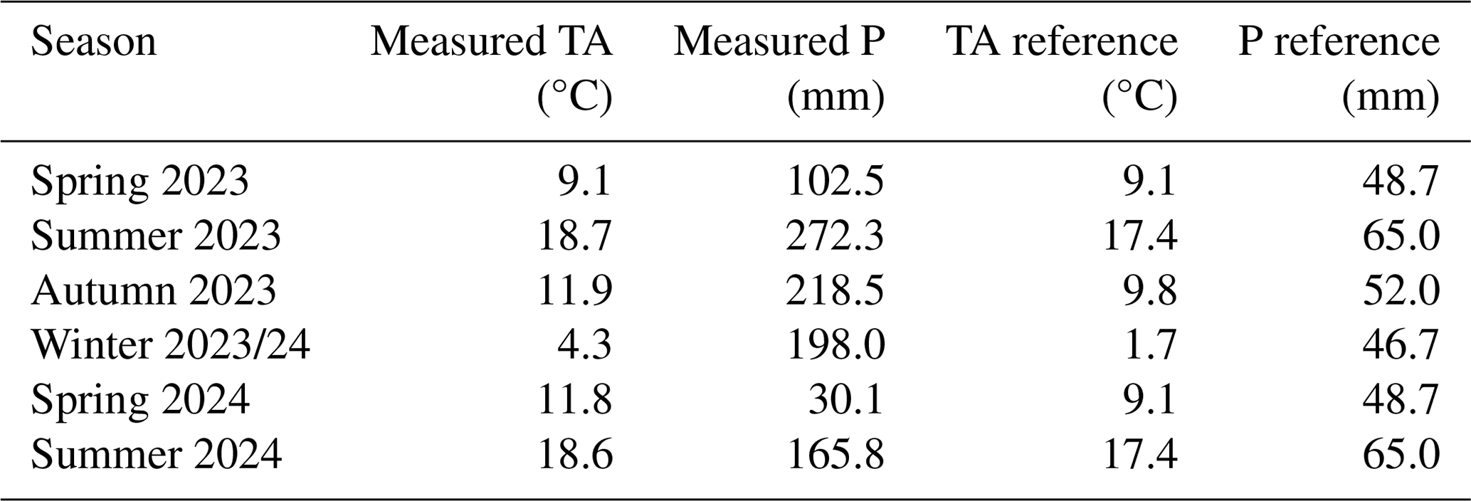
TA followed a seasonal cycle, with the lowest values in winter (daily means between 0 and 10 °C, with occasional lower values) and the highest values in July and August of both 2023 and 2024 (daily means around 20 °C). TA was slightly larger at the OC tower than at the other three AF towers during most of the campaign, with enhanced differences in summer and very small differences in winter. The mean TA during the campaign was 12.86 °C at the OC site, while it was 12.49 °C at the AF site. The three AF stations showed very similar TA values. TA was higher in all seasons compared to the climatological averages (Table 2), except in spring 2023, for which both values were similar (9.1 °C). Summer 2023 and summer 2024 were slightly warmer (18.7 and 18.64 °C, respectively) than the reference value (17.4 °C). Autumn 2023, winter 2023–2024 and spring 2024 were clearly warmer than the climatological averages, with 11.9, 4.3 and 11.8 °C vs. the reference values of 9.8, 1.7 and 9.1 °C, respectively. The absolute difference between measured and historical data was largest in winter.

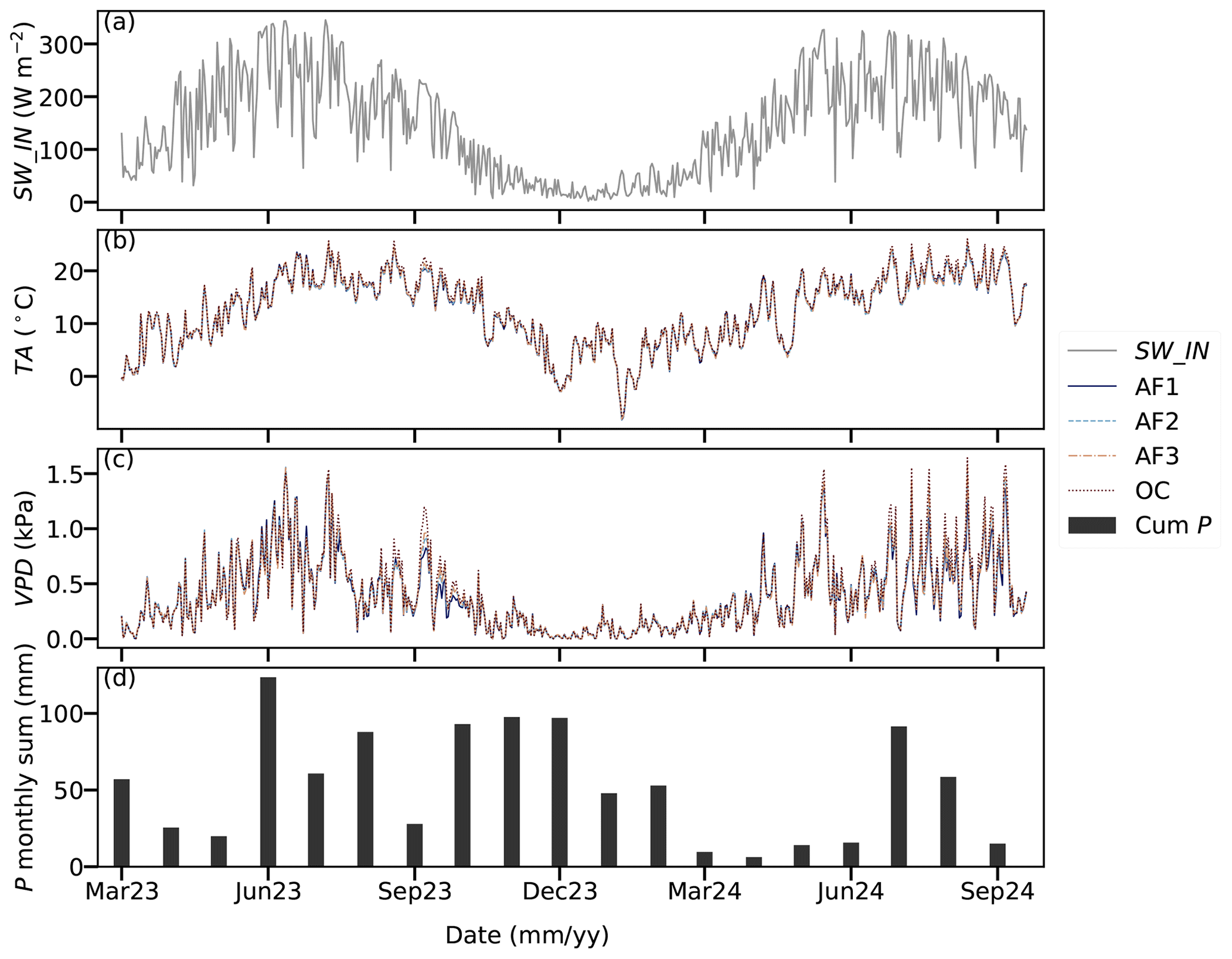
Figure 2 Time series of daily mean meteorological parameter and the cumulative sum of precipitation across the measurement campaign: (a) global radiation (SW_IN), (b) air temperature (VPD), (c) vapour pressure deficit (VPD) and (d) monthly sums of precipitation (P). SW_IN and P were considered to be common to all of the stations because the size of the site is small enough to assume homogeneity in these parameters, whereas TA and VPD were plotted separately for all four stations. Data were filtered for outliers using lower and upper limits; gap-filled as detailed in Sect. 2.3.3; and then aggregated to daily values by taking the daily mean for SW_IN, TA and VPD and the daily sum for P.

VPD values also showed a marked seasonality (Fig. 2c). Values were very low in winter, between 0 and 0.2 kPa, and increased towards summer in both 2023 and 2024, reaching daily means between 1 and 1.5 kPa, while, in the autumn of 2023, VPD was lower, with values of around 0.5 kPa. Comparing the four stations, the OC site experienced a larger VPD from July to October 2023, while, during the rest of the campaign, no significant differences were observed across the stations. The mean VPD was 0.41 kPa at the OC site and 0.4 kPa at the AF site as an average of the three stations. The differences between the three AF stations were very small.

3.2 Footprint climatology

All footprints exhibited larger contributions from the western side of the towers in all periods (growing season of 2023, harvest period of 2023, winter 2023–2024, growing season of 2024 and harvest period of 2024), corresponding to the dominant wind direction at the site (Fig. 3). For all periods under consideration and for both 50 % and 80 % footprint areas, the footprint of the OC tower was smaller than for the three AF towers due to the lower measurement height. At the AF site, footprints decreased from 2023 (Fig. 3a and b) to 2024 (Fig. 3d and e), likely due to the increase in the canopy height of the trees. In the case of the OC site, footprints were similar during the growing season of 2023 compared to the growing season of 2024 (Fig. 3a and d) and smaller during the harvest period of 2023 compared to the harvest period of 2024 (Fig. 3b and e). The 50 % footprint climatology contribution was concentrated in a small area around the stations, covering only the two crop fields at both sides of the stations, plus one or two tree rows in the case of the AF site. There were small variations from season to season and a partial overlap between towers AF1 and AF2 and towers AF2 and AF3.

The 80 % footprint climatology contribution was larger, covering a larger portion of both the AF and OC sites and, therefore, a surface with a larger heterogeneity due to the presence of more diverse crops and/or trees. The three stations at the AF site exhibited partially overlapping footprints for the 80 % footprint climatology, with different sizes and degrees of similarity depending on the evaluated period. The most intense overlap occurred during the growing season of 2023 (Fig. 3a). The 80 % footprint of the three towers covered approximately four tree rows and four crop rows each. The three towers at the AF presented different footprint sizes, with the largest areas being covered by AF3, followed by AF2 and finally by AF1. This rank of magnitude was the same in all seasons. The footprint from the OC tower covered both the western and eastern fields around the tower, but the contribution was larger from the western part in all seasons. For all stations, there were some contributions to the 80 % footprints from the areas beyond the AF or the OC fields, especially remarkable in the case of AF3. However, the contributions of the areas outside the AF site were expected to be negligible with regard to the interpretation of the results.

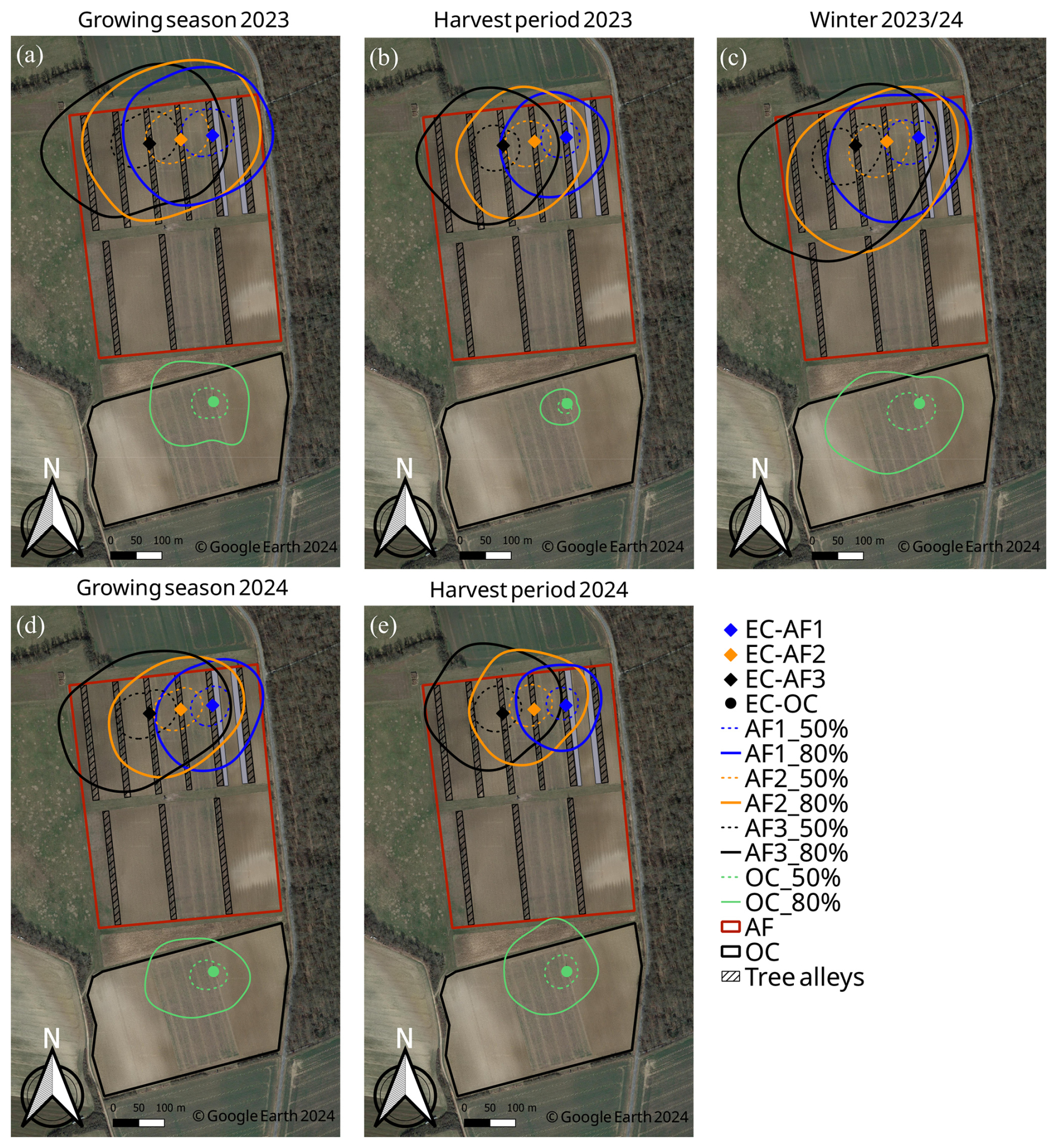
Figure 3 Footprint climatologies, calculated from the model of Kljun et al. (2015), as detailed in Sect. 2.3.4, for the three towers at the AF site (AF1, blue; AF2, orange; AF3, black) and the tower at the OC site (green), divided into five different periods: growing season of 2023 (a), harvest period of 2023 (b), winter period of 2023–2024 (c), growing season of 2024 (d) and harvest period of 2024 (e). The lines plotted in the map represent the 80 % (solid line) and 50 % (dashed line) contribution areas of the footprint. The station locations are marked with diamonds for the AF stations and a circle for the OC station. Figure created with QGIS v. 3.22; aerial map by Google Satellite Maps. © Google Earth 2024.

The analysis of the differences in land cover measured by the different stations revealed seasonal variations. Because all of the AF stations covered some of the tree rows, specifically three or four in the case of AF1 and four to six in the case of AF2 and AF3, the description of the differences will focus on the different crops covered by the 80 % footprints. During the growing season of 2023 (Fig. 3a), the three stations at the AF site covered all crops, whereby AF3 only covered a small portion of the barley field and the nettle fibre. During the harvest period in 2023 (Fig. 3b), AF2 covered all crops, including harvested rapeseed, while AF1 covered corn, barley (harvested at the end of August 2023) and nettle fibre, and AF3 covered rapeseed (harvested) and corn. In winter 2023–2024 (Fig. 3c), all towers covered most of the crop fields, but these were mostly bare soil at this stage. During the growing season of 2024 (Fig. 3e), AF1 covered nettle fibre, rapeseed and barley; AF2 covered all crops; and AF3 covered corn, barley and only a small portion of rapeseed and nettle fibre. Finally, during the harvest period of 2024, AF1 covered nettle fibre, rapeseed (already harvested) and barley (harvested 3 weeks after the beginning of this period); AF2 covered all crops; and AF3 covered corn and barley. In all seasons, the OC tower covered mostly the western field (corn in 2023 and barley in 2024) and partially covered the eastern field (barley in 2023 and rapeseed in 2024).

3.3 Weekly sums of carbon and evapotranspiration

The weekly cumulative sums of FC (Fig. 4a) exhibited a marked seasonal behaviour and similar variability across the four towers. The seasonal cycle was characterized by carbon uptake (negative values) during the growing season and carbon loss (positive values) during winter. The differences were smaller across the three AF towers, with AF1 and AF2 exhibiting more similar behaviour. During the 2023 growing season, there was a strong uptake of around −30 to −40 g C m⁻² per week at all stations from April to September 2023. This was interrupted by a short, 3-week dry period at the end of May and the beginning of June of 2023 (DWD, 2024), during which the AF site turned into a weak carbon source (as measured by AF2) or a weak carbon sink (as measured by AF1 and AF3). AF3 showed stronger uptake until mid-June. After that, OC showed the strongest uptake (−40 to −60 g C m⁻² per week) for the rest of the growing season. After the rapeseed harvest on 13 July 2023, the weekly sums decreased in magnitude but remained substantial at AF1, AF2 and OC (AF3 was missing during this period). Around the barley harvest on 22 August 2023, the sums decreased notably. From October 2023 to March 2024, the values were positive and comparable across all stations, indicating a carbon release from the ecosystems. During the 2024 growing season, carbon uptake diminished compared to the 2023 growing season. The strongest uptake of around −25 g C m⁻² per week occurred in July 2024. AF2 and OC showed the strongest uptake in June and July. However, after the rapeseed harvest on 15 July, the uptake decreased, and AF2 and OC changed to a carbon source. Meanwhile, AF1 and AF3 still showed negative values. After the barley harvest on 5 August 2024, the uptake at AF1 and AF3 decreased further, with AF1 changing to a carbon source. AF3 exhibited a CO₂ sequestration behaviour until the end of the measurement period.

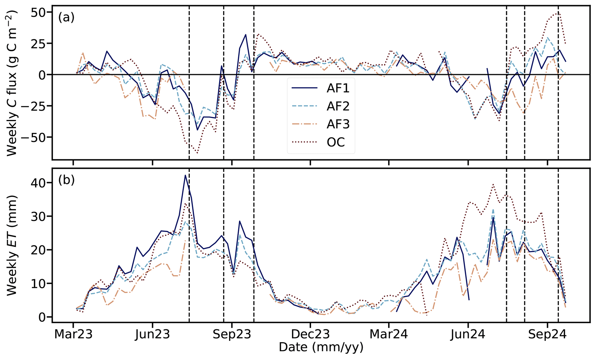
Figure 4 Weekly sums of the net ecosystem carbon exchange as a carbon (C) flux (a) and evapotranspiration (b, ET) measured at the four stations across the measurement campaign. Sums were calculated from the gap-filled time series. Missing values correspond to gaps longer than 2 weeks, which were not considered in the analysis. The horizontal line in sub-plot (a) highlights the zero line, separating the uptake (negative fluxes) from the emission (positive fluxes). Vertical dashed lines represent, from left to right, the harvest dates of rapeseed (13 July 2023), barley (22 August 2023) and corn (26 September 2023) in 2023 and rapeseed (15 July 2024), barley (5 August 2024) and corn (13 September 2024) in 2024. Due to the requirement of taking only gap-filled data for gaps of up to 2 weeks in duration, there were some missing weeks for all stations and two very long gaps, in summer 2023 for AF3 and in winter 2023–2024 for AF1.

The weekly cumulative sums of ET (Fig. 4b) also exhibited a strong seasonality and similar variability across all stations. During the 2023 growing season, the weekly ET sums increased from April (around 10 mm per week) until the maximum values were reached in July, with a magnitude of 30 mm at AF2, AF3 and OC and 40 mm at AF1. Afterwards, there was a progressive reduction in ET, especially enhanced after the rapeseed harvest on 13 July 2023 and the corn harvest on 26 September 2023. AF1 showed the highest values until October 2023. After that, all stations showed low values of around 5 mm per week, coinciding with the winter period, until March 2024. During the 2024 growing season, ET increased progressively at all the stations until reaching the maximum values of 30 and 40 mm. This increase was interrupted only by a reduction in ET in June, more pronounced at the AF towers. After the peak in the growing season, ET was reduced, especially after the rapeseed harvest on 15 July 2024 and the barley harvest on 5 August 2024. The highest values during the 2024 growing season and harvest period were found for the OC site. AF3 exhibited lower values at the beginning of the growing season, but the three towers at the AF site showed good agreement from July onwards.

3.4 Coefficients of variation and spatial and temporal variance

3.4.1 Classification into wind direction bins

The CVs calculated at the half-hourly scale (Eq. 1) were the largest for FC in the eastern and southeastern wind sectors (60–180°) and all of the evaluated periods, followed by the CVs of LE and H (Fig. 5). The largest values of the CVs of FC were reached during the 2023 growing season, reaching up to 8.4. The magnitude of the CVs of FC was comparable to the magnitude of the CVs of LE and H in the other wind sectors and periods, with values of between 0.25 and 0.4. Notably, the CVs of FC were larger during the harvest period of 2024 than during the 2024 growing season. The CVs of WS, USTAR and W_SIGMA were low compared to the CVs of FC, LE and H. The lowest variability across wind sectors in all periods was found for W_SIGMA, followed by USTAR and WS, with CV values below 0.15 in most of the cases.

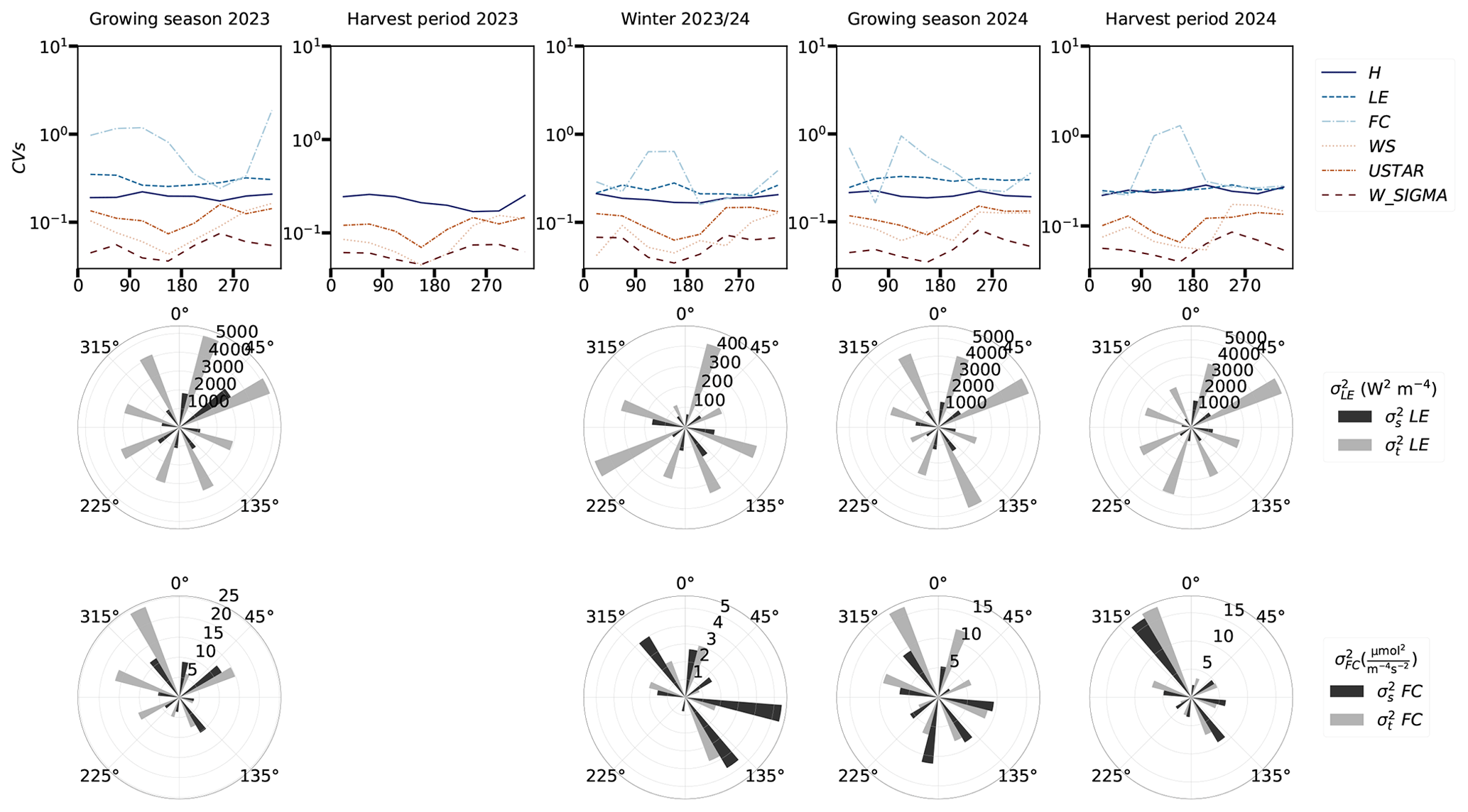
Figure 5 Top row: coefficients of variation (CVs), calculated following Oren et al. (2006), for FC, LE and H, WS, USTAR, and W_SIGMA. Middle row: spatial (σ_s LE) and temporal (σ_t LE) variance for LE. Bottom row: spatial (σ_s FC) and temporal (σ_t FC) variance for FC. Data were grouped in all cases by wind direction bins of 30° each and separated into the five analysis periods (growing season of 2023, harvest period of 2023, winter 2023–2024, growing season of 2024 and harvest period of 2024), detailed in Sect. 2.3.4. Due to the two very long gaps in AF1 and AF3 (see Fig. 4), as well as some shorter gaps, there were no data corresponding to the harvest period in 2023 for FC or LE. Therefore, the sectorial plots for the variance partitioning are missing. Note that, in the first row, due to the large magnitude of some of the CVs of FC, the variability in the lines corresponding to the other variables is more difficult to visualize. Note that the y axis is in a logarithmic scale in the CV plots to facilitate visualization. Note also that the scale is different in the circular plots, depending on the magnitude of what is represented in each season. No gap-filled data were used to create this plot.

For both FC and LE, both variance values were larger during the growing season and the harvest period in both years than during winter due to the larger magnitude of fluxes. Due to the scope of this analysis, it is important to remark in which wind sectors σ_s was larger than σ_t. Looking first at LE (Fig. 5, middle row) σ_s was larger than σ_t only in the sectors of 225–270 and 315–360° during the winter of 2023–2024. For all other wind sectors and periods, σ_s was lower than σ_t.

Regarding FC (Fig. 5, bottom row), the picture was different compared to LE, with a higher relevance of the spatial component of the variance. During the 2023 growing season, σ_s was larger than σ_t in the northeastern sector (0–45°) and the southern half (90–270°). During winter 2023–2024, σ_s was larger than σ_t in all wind sectors. During the 2024 growing season, σ_s was larger than σ_t in the eastern and southern sectors (0–270°). Finally, during the 2024 harvest period, σ_s was larger than σ_t in all sectors, except in the northwest (315–360°).

3.4.2 Classification into weekly intervals

The weekly CVs across the measurement campaign were largest for FC, with a large difference compared to the other evaluated variables (Fig. 6a). The difference was especially remarkable during winter and from March to May in both 2023 and 2024. During most weeks, the CVs of FC ranged between 0.2 and 4.0 but reached high values of around 30 at some specific times of the growing season in both years and during winter. The CVs of FC were much larger than the CVs of LE and H, while in the summer months (after June) and during the harvest period in both 2023 and 2024 the CVs of FC and LE were similar, with values between 0.2 and 0.5, closely followed by the CVs of H. Throughout the entire campaign, the CVs of USTAR and W_SIGMA were much lower than for H, LE and FC, similarly to what is shown in Fig. 5, with values below 0.2 across the entire period. However, the CVs of WS were similar to those of H during the growing season and the 2023 harvest period. After summer 2023, the magnitude of the CVs of WS were reduced. The CVs of USTAR and W_SIGMA were the lowest and did not change much during the campaign. In general, the harvest events did not clearly affect the variation in CVs for all variables.

With regards to partitioning the variance into its temporal and spatial components, σ_t was higher than σ_s for both LE and FC (Fig. 6b and c) during the summer months in both year. During winter and the months of March and April, both variance components were of similar magnitude for LE and FC. The highest variance (for both components) was observed during the end of the growing season in both years and during the harvest period in 2024, while the lowest occurred in winter time. The effect of harvest events in 2024 was shown by a reduction in the difference between σ_t and σ_s compared to previous summer months and a reduction in the variance magnitude (Fig. 6b).

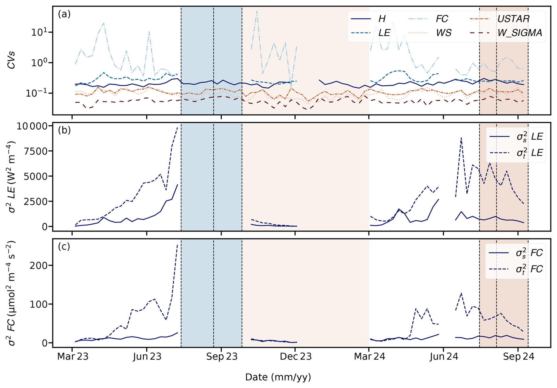
Figure 6 (a) Coefficients of variation (CVs), calculated following Oren et al. (2006), for FC, LE and H, $\overline{u}$, USTAR, and W_SIGMA (logarithmic scale); (b) spatial (σ_s LE) and temporal (σ_t LE) variance for LE; (c) spatial (σ_s FC) and temporal (σ_t FC) variance for FC. The plotted values are weekly means calculated at 30 min temporal resolution from the flux time series. Vertical dashed lines represent, from left to right, the harvest dates of the crops in 2023 for rapeseed (13 July 2023), barley (22 August 2023) and corn (26 September 2023) and in 2024 for rapeseed (15 July 2024), barley (5 August 2024) and corn (13 September 2024). Dashed areas correspond to the 2023 harvest period (dull blue), the winter period (dull yellow) and the 2024 harvest period (dull brown) for a better comparison with Fig. 5. Due to the two very long gaps in AF1 and AF3 (see Fig. 4), as well as some shorter gaps, there were no data corresponding to the harvest period in 2023 for FC or LE, and there were only a few weeks of data in the winter period. Note the logarithmic scale in panel (a), introduced due to the large magnitude of some of the CVs of FC for visualization purposes. No gap-filled data were used to create this plot.

3.5 Effect size and statistical representativeness of the three-tower network

The effect size (d) values were larger in the case of the comparison of LE sums than for the comparison of FC sums (Fig. 7). The values calculated using only the random error as the error in the measured data (Fig. 7a) were larger than the values calculated using the sum of the random and systematic errors as the error in the measured data (Fig. 7b). This is a direct consequence of the inclusion of a larger denominator in Eq. (3).

With regard to effect size, d values were lower in 2023 than in 2024 for FC and LE and in both error cases being considered. For FC, the values of d_AF-MC,FC were larger than the values of d_AF,FC in both years and increased at the end of the growing season and during the harvest period in 2024. In the case of LE, the values of d_AF-MC,LE were lower than the values of d_AF,LE in 2023 but were larger in 2024. The largest values of d were attained during July, August and September of 2024 for LE (magnitudes up to 28), while, in the case of FC, values were largest at the end of the growing season in 2023 (magnitudes up to 12). If only random error was considered, the values of d for LE were larger than those for FC in all periods except for the end of the growing season in 2023 (Fig. 7a). In the case of considering random and systematic errors (Fig. 7b), d values were larger for FC in 2023 and for LE in 2024.

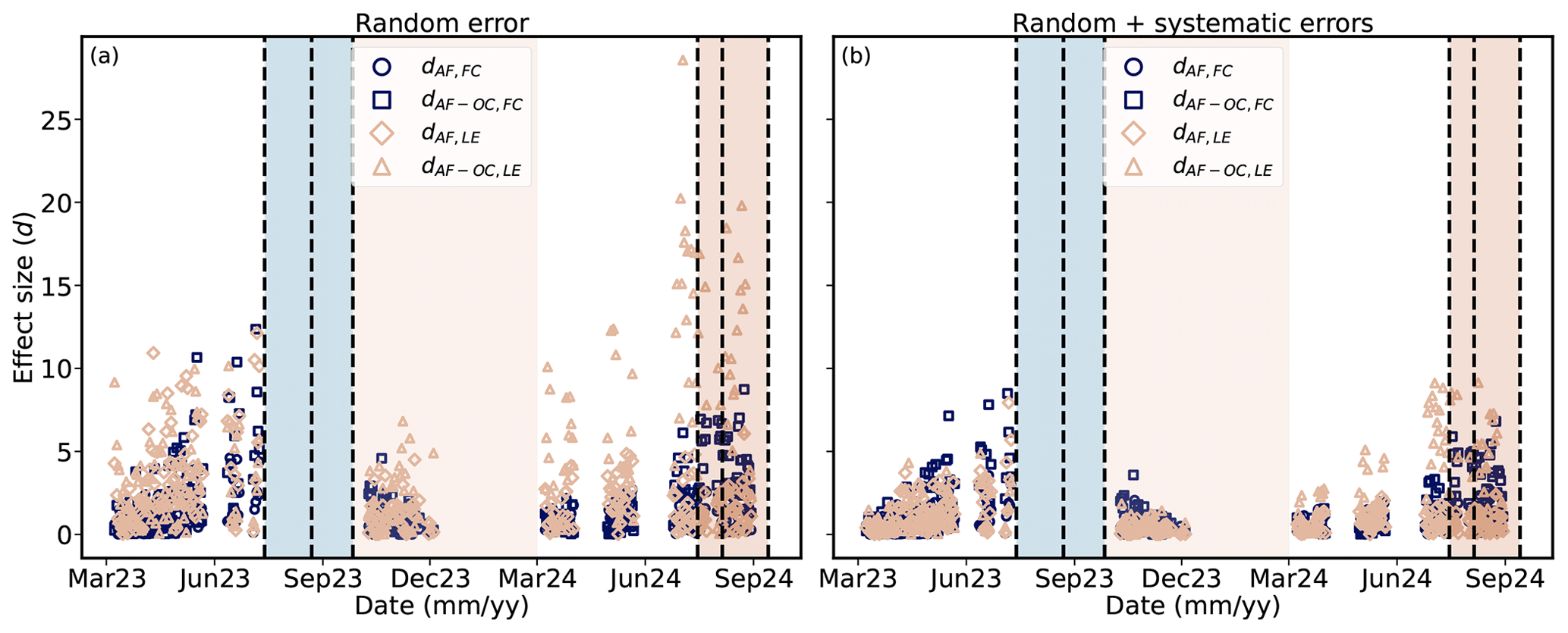
Figure 7 Time series of the effect size (d) for FC and LE, using as the error in the measured data the random error (a) or the sum of the random and systematic errors (b). d was calculated according to Eq. (3), based on the daily sums of FC and LE. Time series of FC and LE had been filtered and gap-filled as described in Sect. 2.3.3, and gaps with a duration over two weeks were excluded from the analysis. Dark blue circles represent the comparison between AF1 and the average of the three stations at the AF (AF1, AF2 and AF3) for the FC. Dark blue squares represent the comparison between the average of the three stations at the AF (AF1, AF2 and AF3) and the OC station for FC. Beige diamonds represent the comparison between AF1 and the average of the three stations at the AF (AF1, AF2 and AF3) for LE. Beige triangles represent the comparison between the average of the three stations at the AF (AF1, AF2 and AF3) and the OC station for LE. Vertical dashed lines represent, from left to right, the harvest dates of the crops in 2023, for rapeseed (13 July 2023), barley (22 August 2023) and corn (26 September 2023); and in 2024, for rapeseed (15 July 2024), barley (5 August 2024) and corn (13 September 2024). Dashed areas correspond to the 2023 harvest period (dull blue), the winter period (dull yellow) and the 2024 harvest period (dull brown), as in Fig. 6.

4 Discussion

4.1 Spatial and temporal variability of FC and LE above the AF system

Using three distributed EC stations over the same AF system, a small spatial variability in meteorological parameters was found, but the spatial variability in CO₂ and energy fluxes was larger. Several rows of trees perpendicular to the main wind direction may potentially influence microclimatic conditions across the AF compared to open croplands (Kanzler et al., 2019), but this AF site (17.3 ha) is smaller than the median farm size (29.4 ha) in Lower Saxony (Jänicke et al., 2022), and the meteorological variables were measured at the AF stations located within the tree strips. These two factors can explain the low variability in meteorological parameters. Therefore, the observed variability in FC and LE should not be attributed to the meteorological drivers but rather to differences in the footprint areas of the three stations. The footprint climatology of the stations partially overlapped (Fig. 3), but the most intense flux contributions originated from a small area around the towers. Differences in crop development and management practices could explain most of the variability in the observed fluxes across the three towers throughout the campaign because of the different crops sown between the tree strips (spatial variability) and the different crop distribution from 2023 to 2024 (temporal variability) (Fig. 1).

The higher spatial variability in turbulent fluxes compared to other turbulence and wind parameters (Fig. 5), especially for FC and LE, was also found in the studies of Katul et al. (1999) and Oren et al. (2006). This can be explained by the complex nature of sources and sinks for CO₂ and H₂O fluxes (Katul et al., 1999) and the effects of landscape heterogeneity (Bou-Zeid et al., 2020). The explanation for the spatial variability in the fluxes is the land cover attribution thanks to the footprint modelling; however, other effects of the heterogeneity were not studied.

The larger CVs of FC at the eastern wind sectors (Fig. 5) during all evaluated periods relate directly to differences in footprint climatology because the footprints differed most at the eastern side of the three AF stations, especially for the 50 % footprint climatology (Sect. 3.2). The harvest events in 2024 did not seem to have a big impact on the CVs (Figs. 5 and 6a), but they reduced the variance magnitude slightly (Fig. 6b and c).

The larger temporal variance, compared to spatial variance, for both FC and LE could be explained by the seasonal and diurnal flux variability, which was more relevant than spatial variability (see Sect. 3.4.1 and 3.5). Nevertheless, σ_t was similar to σ_s in winter for both LE and FC, which can be attributed to the dormant state of the ecosystem, leading to small diurnal variations and, consequently, small temporal variations. In summer 2024, for LE, σ_s was similar to σ_t due to the lower area overlap caused by smaller footprints (Fig. 3) compared to the 2023 growing season. This was also due to the absence of a fully developed crop in the eastern part of the field because of the poor rapeseed growth during this season. This resulted in weaker LE, especially at tower AF1, and led to a lower spatial variation.

In comparison to similar approaches in the literature, Peltola et al. (2015) found a paired temporal and spatial variability in CH₄ fluxes measured at three different heights on a tall EC tower and two additional EC stations over an agricultural landscape. Hollinger et al. (2004) measured fluxes using two towers with non-overlapping footprints in a forest and found that the temporal variability was larger; however, the spatial disagreement in FC was not negligible despite the apparent homogeneity of the studied ecosystem. Rannik et al. (2006) also compared the FC measured from two nearby towers over the same ecosystem, with partially overlapping footprints, and found relevant systematic errors in the daytime fluxes, attributed to the variability in the turbulent flow field caused by the complexity of the terrain. These systematic differences were important for attributing long-term uncertainties in ecosystem carbon uptake, as would be the case in the complex AF site of the present study. Davis et al. (2010) investigated the heterogeneity in FC above arable land and demonstrated the significant impact of spatial heterogeneity on annual carbon balances. Furthermore, Soegaard et al. (2003) quantified the annual carbon budget of an agricultural landscape by combining footprint-weighted fluxes and spatial variability in different crops, demonstrating the large potential of spatial heterogeneity to bias annual flux estimates. In the present study, the influence of different land covers around the towers was detectable for both FC and LE, except during the winter period. However, the differences were smaller than expected for crops with clearly different seasonality. As other effects of heterogeneity on flux measurements cannot be captured with this setup, a first explanation could be the partially overlapping footprints and the buffering effect caused by the presence of the trees. As trees were assumed to behave similarly across the AF site, their similar CO₂ and water fluxes attenuated the potentially larger differences in turbulent fluxes that would be expected among the crops without trees.

The observed variations in the weekly cumulative sums of FC and ET across the campaign (Fig. 4) can be attributed to the developmental and management differences among the crops cultivated around the stations, provided that the trees were growing similarly across the entire AF site. These differences can be directly connected to the previously explained behaviour of the CVs and partitioning of the variance. Spatially replicated experiments demonstrated the potential to more accurately estimate the uncertainty in turbulent fluxes, e.g. by using non-overlapping paired towers, as in Hollinger and Richardson (2005), but this could not be applied in the present study due to the overlapping footprints. Conversely, the deployment of three towers provided a more comprehensive dataset compared to the single-tower approach. However, the choice of the towers location in the present study might not have been optimal (Chen et al., 2011) since footprints were partially overlapping (Figs. 1 and 3). This was due to logistical constraints that precluded the selection of any other location within the AF site, such as in the southernmost part of the field. On the other hand, the purpose of the study was to investigate small-scale variability in the highly heterogeneous AF, a goal that was generally accomplished.

Specifically, the earlier development of rapeseed in 2023 led to an initial carbon uptake at AF3 because the main footprint covered rapeseed (Fig. 3a). This matched the larger CVs of FC on the eastern side of the field (Fig. 5) and during March and April 2023 (Fig. 6a). However, the earlier growth of rapeseed did not increase ET in AF3 (Fig. 4b), leading to comparable CVs of LE for all wind sectors (Fig. 5). This is because rapeseed can maintain a relatively large carbon uptake while using limited water resources (Najibnia et al., 2014). The subsequent development of corn and barley led to similar weekly uptakes of carbon at AF1 and AF2 but a larger ET at AF1, leading to a decrease in the CVs of FC and a modest increase in the CVs of LE. Besides the partially overlapping footprint (Fig. 3), another reason is a different water use efficiency among barley and corn, with this being lower for barley and therefore explaining the similar carbon uptake compared to corn at a higher ET (see, for example, Pohanková et al., 2018). After the short drought in May–June, which affected all three stations by reducing both carbon uptake and ET, weekly carbon uptakes of AF1 and AF2 and weekly ET sums were larger than for AF3 until the harvest period. This can be attributed to corn and barley being less present in the footprint area of AF3 (Fig. 3a). Corn and barley exhibited a more intense physiological activity, immersed in the growing season, while rapeseed was likely to be at its maturity stage.

The rapeseed harvest in 2023 had a negligible effect on the carbon uptake of AF1 and AF2 but seemed to have an effect on ET, which was reduced for both stations. This can be attributed to a period of several precipitation events, low TA and VPD (Fig. 2), which reduced both physiological activity and atmospheric water demand. The barley and corn harvests reduced the carbon uptake and ET. In particular, the corn harvest had a large impact because it was the main crop in the footprints of AF1 and AF2 (Fig. 3b). After the harvest period, the slightly larger difference between the three stations may have been an effect of the larger gap-filling uncertainty due to the longer gaps, agreeing with an enhanced spatial variance compared to the temporal variance (Fig. 6b and c).

In 2024, the very dry spring (Table 2) did not affect weekly sums of ET but reduced the magnitude of the weekly sums of FC compared to 2023. In 2024, there was no earlier development of the rapeseed as this occurred in 2023 due to the very wet winter conditions. The variability in ET was larger than in 2023 due to less overlapping footprints and due to the difference in rapeseed growth (Fig. 3d). The larger carbon uptake at AF2, as well as the larger ET (Fig. 4), during the whole growing season of 2024 can be explained by the influence of barley and, partially, corn, while, at AF1, only parts of the barley field and the non-well developed rapeseed were detected (Fig. 3c). Carbon uptake and ET were smaller at AF3 because corn developed later, but these reached similar values as AF1 once corn started to grow. After the rapeseed harvest, AF1 and AF2 saw both their carbon uptake and ET release being reduced, with AF2 turning into a carbon source. This was explained not by the footprint of AF2 in the rapeseed field (Fig. 3e) but rather by the mature barley and the strong ecosystem respiration under wet conditions. Carbon uptake and ET release at AF3, on the other hand, did not show the effect of the rapeseed harvest because AF3 did not have the corresponding portion of the field measured (Fig. 3e). AF3 maintained a large weekly carbon uptake and similar ET due to the presence of the corn in its footprint area (Fig. 3). Afterwards, the barley harvest reduced the uptake of AF1, turning it into a carbon source, and of AF3; this was also the case for ET due to the footprint covered by both stations (Fig. 3e). Carbon uptake was progressively reduced until it eventually turned into emissions around the corn harvest, which was the main crop in the footprint area of AF3.

4.2 Differences in FC and ET between AF and OC systems

The AF site typically had lower air temperature and higher RH than the OC site (Fig. 2) because the trees at the AF act as a buffer to maintain cooler air temperatures and cooler soil, resulting in a larger RH. This is pointed out in a review by Quandt et al. (2023). The authors stated that, during drought events and under drier and warmer climatic conditions, as projected in future climate scenarios, trees might potentially help in sustaining cooler temperatures and in keeping the air more humid.

Carbon uptake and ET release were enhanced at the AF site at the beginning of the 2023 growing season because of the earlier development of the trees and the rapeseed, both present in the footprint of all three AF stations (Figs. 1 and 3a), while the OC station measured mostly corn (Fig. 3a). Corn is a crop with a later development compared to barley or rapeseed (Lokupitiya et al., 2009; Soegaard et al., 2003), but it is typically very productive (Hollinger et al., 2005; Lokupitiya et al., 2016). Therefore, carbon uptake was larger at the OC site during most of the 2023 growing season after corn started to grow, which occurred later than for rapeseed and barley. A similar ET between OC and AF2 (Fig. 4b) indicated a larger water use efficiency at the OC site. In our study, the short dry period in May–June 2023 took place before corn reached its peak growth stage, while rapeseed and barley were in a more advanced stage and were more affected by the dry conditions. In general, the whole campaign took place during very wet conditions. This might have increased the ecosystem respiration because it led to more soil organic matter decomposition driven by larger litter amounts at the AF site. This, together with a larger respiration from the trees, can explain why AF2, even though it was surrounded by corn, did not take up as much carbon as the other towers in the AF system.

During the 2023 harvest period, the footprint of the OC station was limited to corn and not rapeseed (Fig. 3b). Corn continued to grow in July and August 2023 at the OC site, which explains why, at the OC site, a very large carbon uptake and ET release were observed, while AF2 and AF1 showed reduced fluxes. In winter, the ecosystems were dormant, which explains the small differences between the AF and OC sites. However, fluxes were very small in magnitude, and it was difficult to observe differences between sites.

During the 2024 growing season, carbon uptake at the OC site was similar to that at the AF site, but ET was larger at the OC site, opposite to what occurred in 2023. This could be explained by barley grown in the main footprint area of the OC (Fig. 3d), as well as in a portion of the rapeseed field, which did not grow well in 2024. Barley is a crop with less intense physiological activity and lower water use efficiency than corn (Pohanková et al., 2018). This explains the smaller differences compared to the AF stations in terms of C uptake and the much larger ET. Also, the meteorological conditions were very wet in winter, with a dry spring. During the harvest period in 2024, the carbon uptake and ET were reduced more sharply at the OC site than at the AF site after the rapeseed harvest because of its partially contributing footprint (Fig. 3e). The reduction was more pronounced after the barley harvest, which contributed the most to the footprint covered by the station.

4.3 Effect size and spatial representativeness of the distributed network

The effect size d is a measure of the relative difference of two variables for two different populations (in this case, two ecosystems or towers within an ecosystem) with respect to the pooled standard deviation of the two populations. The interpretation of the calculated values was done according to Fig. 3 in the paper by Hill et al. (2017), where the number of EC replicates over an ecosystem or for comparing two ecosystems was estimated based on the desired statistical power (from 0 to 1) and the effect size value. The statistical power related to the confidence in the accuracy of the measurements, such that a value of 1 means we can be 100 % certain about the measured differences.

In the case of comparing the AF stations, similar values for both LE and FC were attained, mostly between 0 and 5. Values of 5 meant that, with three towers, a statistical power between 0.7 and 0.95 was achieved; however, with values close to 0, the statistical power dropped dramatically so that no confidence in the accuracy of the differences could be drawn. In the case of comparing AF-MC setups, d values were larger than for the comparison of the AF stations, which meant that a larger statistical power was achieved because the daily sums were larger than the pooled uncertainty. Values larger than 2 or 3 – in many cases, reaching up to 15 or 20 – denoted a statistical power above 0.975 and, therefore, a very large confidence in the daily sums. Furthermore, d_LE was larger than d_FC, meaning that the statistical confidence was larger for LE. When using random and systematic errors as the errors attributed to measured data (Fig. 7b), d values were much lower. This matches the interpretation of Hill et al. (2017): if the EC systems are too uncertain, the number of systems needed to achieve a large statistical power (above 0.9) increases exponentially. If the LC-EC setups used in this study were to be a lot less accurate, e.g. with 2 times more systematic error compared to conventional EC, the effect size values would be too low so that no certainty about the data could be ensured, unless the number of towers were to increase in order to counteract the loss of accuracy.

Several studies addressed the spatial representativeness of fluxes and footprint climatology. These studies focused on studying RE (Hollinger and Richardson, 2005), separating ecosystem structure and sampling errors in the spatial variability of fluxes (Oren et al., 2006), disentangling the temporal and spatial variability of fluxes using a single-tower approach and footprint modelling (Levy et al., 2020; Soegaard et al., 2003), the representativeness of single-point measurements at the pixel scale for regional- to global-scale models (Chasmer et al., 2009; Chen et al., 2009; Wang et al., 2016; Ran et al., 2016), or studying the effect of diverse meteorological conditions in the footprint climatology and canopy structure (Abdaki et al., 2024). To the best of our knowledge, the study of Cunliffe et al. (2022) was the only one that deployed several LC-EC setups similar to those used in our study and one additional conventional EC setup to quantify the impact of landscape heterogeneity on turbulent fluxes. They studied a dryland site with very low flux magnitudes, which is different from our site. They obtained a useful agreement between different LC-EC setups and conventional EC setups and attributed the differences between setups to the ecosystem heterogeneity, covered by different bushes and grass species. However, a less detailed analysis of the spatial and temporal variability of the fluxes was performed.

In the EC community, EC replicates are uncommon (Hill et al., 2017; Stoy et al., 2023). Therefore, the effect size of either the means or sums of fluxes is typically not estimated. Hill et al. (2017), as the first paper showing the potential of LC-EC setups in increasing spatial replication in EC studies, estimated the effect size by comparing the average carbon sequestration and the standard deviation of the cumulative sums for ideal and non-ideal FLUXNET sites (Baldocchi, 2014). In the present study, the effect size was calculated similarly but based on daily sums and pooled standard deviations (errors) of the 30 min time series. The concept in Hill et al. (2017) was different since measurement errors tend to decrease relative to the aggregation period when cumulative sums are calculated (Moncrieff et al., 1996). Their calculated standard deviation was based on the uncertainty in the cumulative sums of the half-hourly carbon fluxes rather than on time series with a higher temporal resolution (30 min). These time series are commonly characterized by higher variability and a potentially lower effect size.

In general, there is still an ongoing discussion on how much the landscape heterogeneity affects balances of carbon and H₂O measured by single EC towers. The LC-EC setups could help to bridge the gap of low spatial replication across such heterogeneous sites by allowing the installation of multiple setups due to their reduced cost. This could be complementary to other methodologies developed to understand the effect of spatial heterogeneity on fluxes measured from single towers, such as in Levy et al. (2020) or Griebel et al. (2016), or measured with several conventional EC setups (Soegaard et al., 2003; Hollinger et al., 2004; Katul et al., 1999; Oren et al., 2006).

4.4 Heterogeneity as a challenge to EC measurements and footprint modelling

As mentioned in the Introduction, the heterogeneity in the surface properties of a certain ecosystem induces horizontal advection, secondary mesoscale circulations and non-equilibrium turbulence processes (Bou-Zeid et al., 2020). Horizontal advection at different spatial scales can distort flux measurements (Cuxart et al., 2016). Furthermore, the dynamics of the roughness sublayer (RSL), defined as the atmospheric layer influenced by the roughness elements and located below the inertial sublayer (Katul et al., 1999), can be modified by the wind barrier of trees at the AF site (van Ramshorst et al., 2022). Upon a change in the underlying surface, an internal equilibrium layer (IEL, Brutsaert, 1998) and an internal boundary layer (IBL, Garratt, 1990) develop. Multiple IELs and IBLs can develop if there are multiple transitions in the surface, such as at the AF site (Bou-Zeid et al., 2020). At the AF site, the major change in the surface is represented by the tree rows (Markwitz, 2021). These rows create persistent waves that enhance the differences in the turbulence-related parameters WS, USTAR and W_SIGMA, though these changes are less pronounced than flux variations. Furthermore, the classical tests of stationarity and equilibrium may fail if the EC station is placed above the IEL (Mahrt and Bou-Zeid, 2020) due to a disequilibrium between the mean flow, turbulence and the new surface (Bou-Zeid et al., 2020). Additionally, the complex canopy structure at the AF site could lead to significant carbon and energy storage, particularly at the crop–tree interfaces and within the dense tree rows. These storage terms may influence advection in the horizontal and vertical directions (Mammarella et al., 2007; Aubinet et al., 2010; Feigenwinter et al., 2008). These effects may affect the turbulence and flux measurements; however, they could not be quantified with the current setup.

The footprint size and the overlap between footprints decreased between 2023 and 2024 due to tree growth (Fig. 3). Combined with changes in crop development and meteorological conditions, this increased the spatial components of the variance for FC and LE (Fig. 5). While the three towers at the AF site had partially overlapping 80 % footprint climatology areas (Fig. 3), the main footprint contributions were concentrated in the immediate areas around each tower (Kljun et al., 2002). Therefore, most of the flux variability can be attributed to land cover differences around the stations. The three-tower network helped disentangle the effects of management activities (e.g. crop harvest) and provided insights into small-scale features caused by the alternating structure of the AF site. The division of the data into wind direction bins, as done in, for example, Kutsch et al. (2005), to address spatial variability in fluxes and turbulence parameters, as well as the spatial and temporal components of the variance, complemented the information provided by the footprint maps.

The footprint model used in the present study (Kljun et al., 2015) allowed us to understand, at a basic level, where the source and sink areas of CO₂ and H₂O were located. Nevertheless, the parameterization of the footprint model does not consider the effects of spatial heterogeneity on the basic parameters of roughness length and USTAR or how canopy heterogeneity influences wind speed and turbulence dynamics within the AF site (Markwitz, 2021). Due to the structure of the AF site, the footprint model likely overestimated the footprint area by attributing sources and sinks to areas that do not actually contribute to the flux. Additionally, footprint estimates are sensitive to the vertical distribution of sources and sinks within the canopy and to the time that air parcels spend within it (Launiainen et al., 2007; Prabha et al., 2008). This is likely to be happening at this AF site due to the structure of the tree rows. Implementing the aerodynamic canopy height following Chu et al. (2018) helped to partially account for the heterogeneity of the AF site in the footprint modelling, but this procedure was also limited. More accurate footprint estimates could be obtained by combining flow dynamics and spatial structure information using large-eddy simulations (Markwitz, 2021; van Ramshorst et al., 2022), with a more advanced footprint modelling, as described in, for example, Göckede et al. (2006) to account for the spatial heterogeneity in roughness length and USTAR. Additionally, aggregating the footprint climatology based on weighted footprints, as in Chen et al. (2009), would allow for a more detailed characterization of the sources and sinks of carbon and water vapour.

Furthermore, the sensor location bias, defined as the uncertainty caused by measuring at only one point above a heterogeneous site, depends on the stability conditions (Chen et al., 2011). Under more unstable conditions, the footprint size decreases, and the location bias of each tower increases. This justifies the use of multiple EC towers to sample an entire ecosystem more effectively. A more detailed study of stability regimes, footprint size and spatial variability of fluxes would inform us about this feature. However, this was not performed in this study due to the limited data availability and the difficulty in gap-filling turbulence parameters needed to classify stability regimes, such as Obukhov length. With longer time series and more complete turbulence and footprint information, some of the previously detailed shortness of this study could be addressed.

4.5 Errors in FC, LE and H

Errors affecting flux calculations are difficult to disentangle because they propagate throughout the entire processing routine, from raw data measurements to final flux corrections. Therefore, the uncertainty in the measured fluxes from the LC-EC setups was assigned based on the random error and the previous inter-comparison studies of Callejas-Rodelas et al. (2024) and van Ramshorst et al. (2024), as detailed in Sect. 2.5. This procedure is similar to the approach applied in Peltola et al. (2015), where they used a previous instrument cross-comparison campaign (Peltola et al., 2014) to assign instrumental uncertainty to the setups they deployed. However, the uncertainty in the use of LC-EC setups, defined in relation to conventional EC, was obtained during a specific campaign and under specific site conditions with the same footprint area; therefore, there might be a bias in the LC-EC error attribution. Additionally, as explained in Sect. 2.5, the uncertainty in the gap-filled fluxes was calculated by assigning individual errors to the 30 min fluxes, which can then be propagated when performing the daily cumulative sums. This was detailed as an initial method for easily evaluating and propagating errors through cumulative sums when comparing new EC setups to conventional EC setups and calculating carbon or ET balances using gap-filled data. Other approaches, as described in, for example, Richardson and Hollinger (2007), could potentially be applicable to this dataset as well.

Including all gap-filled data, with some very long gaps, particularly affecting AF3, would have made the analysis more uncertain (Lucas-Moffat et al., 2022). Therefore, only measured data and gaps shorter than 2 weeks were used, although this did not permit a more complete spatial heterogeneity study throughout the campaign. The optimal solution for this study was to use a combination of REddyProc for short gaps and the XGBoost model for long gaps, similarly to what was done in Winck et al. (2023). This solution allowed us to assign individual errors to each 30 min flux, as explained in Sect. 2.5. Additionally, applying more strict filtering criteria, such as a higher USTAR threshold or a lower quality flag, would provide higher-quality data but would also increase uncertainty due to the filling of more gaps.

We used TA, SW_IN and VPD as predictors for gap-filling, which are generally recognized to be the main drivers of CO₂ and H₂O fluxes (Vekuri et al., 2023; Wutzler et al., 2018). WS was used because of its influence on turbulence development and the spatial information carried by eddies, especially above a very rough surface, such as at the AF site. Wind direction was selected to account for the spatial heterogeneity across the different measurement locations of the towers (Richardson et al., 2006). Other meteorological variables were either less relevant for the analysis, such as atmospheric pressure, or more complex to gap fill, such as net radiation.

5 Conclusions

This study presents, for the first time, 1.5 years of measurements from a distributed network of three eddy covariance towers above a temperate heterogeneous agroforestry system, as well as a comparison to an adjacent, open-cropland agricultural system. Using three eddy covariance stations allowed us to capture the spatial and temporal variability across the site, which particularly affected carbon flux. The main differences were attributed to the different developmental stages of the crops across seasons, with larger disturbances in carbon flux and latent heat flux after harvest events. Due to the high degree of spatial heterogeneity, a broader footprint coverage was necessary to capture small-scale differences at the agroforestry site. Furthermore, binning the data by wind direction sectors and weeks provided a detailed picture of the temporal and spatial components of the variance and the coefficients of spatial variation. This was important because the differences between stations were small enough to be masked by a less resolved analysis.

Secondly, this study incorporated a complex gap-filling procedure that complemented previously published recommendations on working with lower-cost eddy covariance data. The datasets gathered during the campaign and the processing scheme added value to the data collection of the project from previous years from several agroforestry and open-cropland sites. Future research will address the contrast between different agroforestry and open-cropland sites in more detail, using more years of data under a broader range of meteorological conditions.

Finally, the footprint coverage required to capture the spatial heterogeneity across the agroforestry site and within the agroforestry and open-cropland sites was improved by using lower-cost eddy covariance setups. We satisfactorily proved the hypothesis that the degree of uncertainty introduced by using slower-response gas analysers for CO₂ and H₂O was counteracted by the better representation of all processes occurring within the agroforestry system. Therefore, we recommend installing multiple eddy covariance setups, including lower-cost setups, whenever the degree of heterogeneity of an ecosystem is large. Future studies could benefit from comparing overlapping and non-overlapping measurements in terms of footprints.