On the challenges of retrieving phytoplankton properties from remote-sensing observations

Remote-sensing satellites provide the only means to observe the entire ocean at high-temporal resolution. Optical sensors assess ocean color through estimates of remote-sensing reflectance (R_rs(λ)). We emphasize a physical degeneracy in the radiative transfer equation that relates R_rs(λ) to the absorption and backscattering coefficients (a(λ), b_b(λ)) known as inherent optical properties (IOPs). This degeneracy stems from R_rs(λ) depending on the ratio $b_{\mathrm{b}}\left(\mathit{\lambda }\right)/a\left(\mathit{\lambda }\right)$, preventing the independent retrieval of non-water IOPs without prior knowledge. We demonstrate that multi-spectral satellite observations lack the statistical power to recover more than three parameters describing non-water absorption and backscattering. Due to exponential-like absorption by colored dissolved organic matter and detritus at shorter wavelengths, multi-spectral R_rs(λ) data cannot detect phytoplankton absorption without strict priors, leading to biased and uncertain estimates. These results challenge decades of IOP retrieval literature, including assessments of phytoplankton growth and biomass. While hyperspectral observations hold promise to recover additional parameters, significant hurdles remain in accurately quantifying IOPs and phytoplankton biomass at a global scale.

1 Introduction

Phytoplankton play essential roles within our ecosystem, serving as the base of the ocean food web and performing ∼50 % of all photosynthesis on Earth. Therefore, assessing phytoplankton growth and death – especially in a changing climate (Behrenfeld et al., 2016; Flombaum et al., 2020) – is critical to any effort to track and predict the health of our planet. Decades of phytoplankton research has revealed significant regional variations in these process and demonstrated that phytoplankton are highly dynamic on relatively short timescales (hours to weeks, especially in coastal areas due to tides, upwelling, pulses of freshwater inflow, and other episodic events (e.g., Cloern and Jassby, 2010)). Therefore, to identify any long-term trend, one must first develop a detailed picture of the variations on seasonal and shorter timescales.

Unfortunately, our ability to measure phytoplankton in situ is greatly hampered by the vast expanse of the ocean. Measurements with high temporal frequency can only be acquired at select, fixed stations such as OceanSITES (Boss et al., 2022). Therefore, oceanographers have turned to remote-sensing satellite observations to perform high-cadence global analyses of the ocean surface. Beginning with the Coastal Zone Color Scanner experiment (Hovis et al., 1980), multi-band observations in optical channels have enabled the inference of phytoplankton and other seawater constituent properties, such as chlorophyll-a concentration and absorption by colored dissolved organic matter (CDOM) and detritus (IOCCG, 2000; Siegel et al., 2002). These properties are obtained from satellite-derived remote-sensing reflectance:

$$\begin{array}{}\text{(1)}& R_{\mathrm{rs}}\left(\mathit{\lambda }\right)\equiv {\displaystyle \frac{L_{\mathrm{w}}\left(\mathit{\lambda }\right)}{E_d\left(\mathit{\lambda }\right)}},\end{array}$$

with L_w the water-leaving radiance and E_d the incident solar irradiance. Their retrieval relies on recovering the absorption coefficient:

$$\begin{array}{}\text{(2)}& a\left(\mathit{\lambda }\right)\equiv {\displaystyle \frac{\mathrm{d}A\left(\mathit{\lambda }\right)}{\mathrm{d}r}},\end{array}$$

with A(λ) the fraction of incident power absorbed and the backscattering coefficient of

$$\begin{array}{}\text{(3)}& b_{\mathrm{b}}\left(\mathit{\lambda }\right)\equiv {\displaystyle \frac{\mathrm{d}B\left(\mathit{\lambda }\right)}{\mathrm{d}r}},\end{array}$$

with B(λ) the fractional incident power scattered out of the beam, which govern R_rs(λ) and are known as inherent optical properties (IOPs).

The underlying physics for IOP retrievals is radiative transfer: the absorption and scattering of sunlight by seawater modulates and directs incident sunlight back to the satellite. While the radiative transfer physics is straightforward (but not simple; Mobley, 2022), there are many factors that complicate the calculations. These include but are not limited to the concentration of the constituents (typically the desired unknown), their variation with depth, the precise wavelength dependence of the absorption and scattering coefficients of each constituent, and the geometric factors associated with the Sun's location relative to the satellite. In addition, Earth's atmosphere attenuates the signal and introduces a dominant background radiation field that must first be estimated and subtracted (“corrected”), which fundamentally limits the precision of any space-based R_rs(λ) estimation (e.g., Frouin et al., 2022).

For decades, researchers have attacked this radiative transfer problem to attempt retrievals of scientifically valuable quantities, including an estimate of the phytoplankton biomass. There is robust and well-founded literature describing (and performing) the translation of apparent optical properties (AOPs, e.g., R_rs(λ)) into inherent optical properties (IOPs; a(λ), b_b(λ)) that depend solely on the water constituents and the water itself. Ideally, one first parameterizes and then estimates (“retrieves”) the absorption and backscattering spectra of the non-water component a_nw(λ), b_b,p(λ) and then infers concentrations or proxies for phytoplankton, CDOM, detritus, etc. From these, one may examine the geographic distribution and temporal evolution of fundamental biological processes across the global ocean (e.g., Behrenfeld et al., 2005; Siegel et al., 2014; Fox et al., 2022).

During the development of a diverse set of IOP retrieval algorithms for this purpose (see Werdell et al., 2018, for a review), the ocean optics community has acknowledged key challenges in the problem that are largely independent of those associated with radiative transfer. These include uncertainties related to the atmospheric corrections, non-uniqueness between common constituents (e.g., CDOM and detritus), and retrieving multiple unknowns from limited datasets (e.g., multi-spectral observations). A few sparsely cited works have also highlighted a more fundamental obstacle to the process: a physical “ambiguity” in the inversion of the radiative transfer equation (Sydor et al., 2004; Defoin-Platel and Chami, 2007). Unfortunately, this problem has often been confused or conflated with the statistical limitations of an insufficient number of bands measuring R_rs(λ) (Werdell et al., 2018; Cetinić et al., 2024). As such, while the community has acknowledged challenges to IOP retrievals from remote-sensing observations, rigorous assessment of the algorithms themselves has been limited and usually only performed in the context of comparisons to sparse in situ observations (e.g., Lee, 2006; Seegers et al., 2018).

Another fundamental aspect of the problem is that we do not know the optimal basis functions that describe a(λ) and b_b(λ), nor even the complete set (e.g., Garver et al., 1994). Indeed, it is an aspiration within the ocean color field to recover (or even discover) the composition of phytoplankton communities (e.g., Mouw et al., 2017). The ocean color research community has hoped that the main limitation is the sparsity of existing multi-spectral bands provided by current satellites and that hyperspectral observations will lead to a major breakthrough. Indeed, Cael et al. (2023) have demonstrated its limited information content from a data-driven analysis of R_rs(λ) spectra, i.e., only ∼2 degrees of freedom in multi-spectral satellite observations. But they also concluded that in situ hyperspectral datasets provide only 1 or 2 additional degrees of freedom to describe the seawater composition. In this paper, we examine this question from a new angle – with the standard approach of IOP retrievals – and reach similar conclusions.

Here, we introduce the Bayesian INferences with Gordon coefficients (BING) package for ocean retrievals in a Bayesian context (see Erickson et al., 2020, 2023, for a complementary Bayesian approach). Our approach follows many of the standard assumptions of widely adopted algorithms in the literature, e.g., the generalized IOP (GIOP) model (Werdell et al., 2013) and the Garver–Siegel–Maritorena (GSM) algorithm (Maritorena et al., 2002). In addition, we emphasize and expand upon the “ambiguity” problem – a physical degeneracy in the radiative transfer equation that couples reflectances to IOPs – which fundamentally limits IOP retrievals. In turn, we demonstrate that IOP retrievals from multi-spectral datasets constrain at most three parameters describing a_nw(λ) and b_b,p(λ). Consequently, if the spectral shape of CDOM absorption is allowed to vary and remains unconstrained, it becomes challenging, even impossible, to independently retrieve phytoplankton absorption with high confidence. This limitation applies to previous satellite missions equipped with multi-band sensors, emphasizing the need for additional constraints or improved observational capabilities for more accurate phytoplankton absorption retrievals. We then examine the prospects for IOP retrievals with hyperspectral observations and discuss additional opportunities to address the deep degeneracies that lurk within.

2 Methods

2.1 Bayesian formalism

At the heart of our analysis is an open-source Bayesian inference algorithm developed for the retrieval of IOPs from remote-sensing reflectances, the BING package. The primary motivations for introducing a Bayesian framework are threefold:

• i.

  it forces one to explicitly describe all of the priors that influence the result;

• ii.

  it leverages well-developed techniques to assess error and correlations in the results without requiring Gaussianity¹, i.e., the assumption that errors, uncertainties, or distributions of the retrieved parameters follow a Gaussian (normal) distribution; and

• iii.

  it permits well-established approaches for performing model selection, i.e., estimating the maximum number of free parameters one can use to describe the data.

BING is conceptually similar to the algorithm presented in Erickson et al. (2020) to analyze diatoms and Noctiluca scintillans, although BING adopts a Monte Carlo Markov chain sampler. In addition, the code base incorporates several previous inference algorithms (e.g., GSM, GIOP) and is extensible to any new user-driven parameterization of the IOPs. The BING package is purely Python and is available on GitHub (Prochaska, 2024).

Provided that there is a forward model (described in the following section) and a parameterization of a(λ) and b_b(λ), the Bayesian inference is straightforward, and a wealth of well-trodden approaches and software packages are available. For BING, we adopt the Monte Carlo Markov Chain (MCMC) formalism, which empirically derives the posterior probabilities for the a(λ), b_b(λ) parameterization P(X|Y), including full uncertainties and all of the cross-correlation terms. This requires the definition of a likelihood function P(Y|X), which will have the form

$$\begin{array}{}\text{(4)}& P\left(Y\right|X)\propto \exp \left\{-{\displaystyle \frac{\mathrm{1}}{\mathrm{2}}}[Y-H(X\left){]}^{\mathrm{T}}C\right[Y-H\left(X\right)]\right\},\end{array}$$

where Y represents the measured R_rs(λ) values, C is the full covariance matrix of R_rs(λ) including correlations, and H(X) is the forward model of R_rs(λ) at the locations of Y.

It can be shown that an MCMC analysis converges to the exact solution if run for an infinitely long time; in practice, the calculations tend to converge after ≈10 000 iterations. For the analysis here, we generally run 75 000 trials with at least 2 walkers per parameter (and at least 16 walkers) and only analyze the last 7000 iterations of each. This release of BING uses the EMCEE sampler (Foreman-Mackey et al., 2013), which was developed for astrophysical applications and has seen widespread adoption in the field (over 8000 citations).

We have also implemented standard χ² minimization (Levenberg–Marquardt; L–M) as a fitting option to speed up model development and portions of the analysis. This also enables one to implement standard inference models in the literature (e.g., GSM and GIOP), which generally use L–M optimization.

Note that the Bayesian approach in BING involves using Bayes' theorem to update the probability of a hypothesis based on prior knowledge and new data. When retrieving IOPs from R_rs(λ), this approach explicitly incorporates all available prior information about the IOPs and their uncertainties into the model. By doing so, it allows for a more transparent and rigorous estimation process. The Bayesian framework considers the likelihood of the observed R_rs(λ) given the IOPs and combines it with the prior probability distributions of the IOPs to obtain a posterior distribution. This posterior distribution provides a probabilistic solution to the inverse problem, highlighting the most likely values of the IOPs while quantifying the uncertainties, leading to more reliable and informed retrievals.

In reference to the detection of phytoplankton, we consider a series of models with and without a_ph(λ) absorption. We then examine the evidence for models with a_ph(λ) in the Bayesian context by applying standard approaches for model selection, i.e., assessing the balance between model fit and complexity. Specifically, we have evaluated the Akaike and Bayesian information criteria (AIC, BIC), which are akin to χ²-difference tests (Bentler and Bonett, 1980):

$$\begin{array}{}\text{(5)}& \mathrm{AIC}=\mathrm{2}k-\mathrm{2}\ln \mathcal{L},\end{array}$$

and

$$\begin{array}{}\text{(6)}& \mathrm{BIC}=k\ln n-\mathrm{2}\ln \mathcal{L},\end{array}$$

with n the number of R_rs(λ) measurements and ℒ the likelihood function calculated assuming Gaussian statistics for uncertainties σ(R_rs(λ)). The likelihood function ℒ quantifies the probability of observing the data given the specific forward model and its parameters. Since it is calculated under the assumption of Gaussian (normal) statistics for the R_rs(λ) uncertainties, this means that the observed data, i.e., the R_rs(λ) measurements, are assumed to be normally distributed around the model predictions with the standard deviation. For our hyperspectral analysis where n≫10, BIC offers a more stringent constraint, but the results with AIC are qualitatively similar. A high AIC or BIC value implies that the model is less likely to be the best model given the data, considering both fit and complexity. Quantitatively, we assess model selection by evaluating the difference in BIC for any two models:

$$\begin{array}{}\text{(7)}& \mathrm{\Delta }{\mathrm{BIC}}_{i,j}={\mathrm{BIC}}_i-{\mathrm{BIC}}_j,\end{array}$$

where $\mathrm{\Delta }{\mathrm{BIC}}_{i,j}<\mathrm{0}$ indicates that model i is preferred and vice versa.

2.2 Radiative transfer with a physical degeneracy

To construct any such algorithm, one must have a well-defined forward model to predict the observables, here remote-sensing reflectances R_rs(λ). For IOP inversion, this means a radiative transfer model – or its approximation – which estimates R_rs(λ) from a(λ) and the backscattering coefficients b_b(λ). The majority of IOP retrieval algorithms developed by the community have used the quasi-single-scattering approximation originally introduced by Hansen (1971) and translated to ocean color by Gordon (1973) (see also Zege et al., 1991). This approach was refined further by Gordon (1986), who approximated the sub-surface remote reflectances r_rs(λ) with a Taylor series expansion:

$$\begin{array}{}\text{(8)}& r_{\mathrm{rs}}\left(\mathit{\lambda }\right)=\sum _{i=\mathrm{1}}^N{G}_{i}u(\mathit{\lambda }{)}^i,\end{array}$$

with

$$\begin{array}{}\text{(9)}& u\left(\mathit{\lambda }\right)\equiv {\displaystyle \frac{b_{\mathrm{b}}\left(\mathit{\lambda }\right)}{a\left(\mathit{\lambda }\right)+b_{\mathrm{b}}\left(\mathit{\lambda }\right)}}.\end{array}$$

Most IOP retrieval algorithms have taken N=2 and set the coefficients to constants, G₁=0.0949 and G₂=0.0794, i.e., values independent of wavelength. In this paper and for the default mode of BING, we adopt the same prescription and coefficients and scrutinize the accuracy of this assumption in Appendix A. For the results in the main text, we assume a perfect forward model; i.e., we use Eq. (8) to generate the target r_rs(λ) and perform the fits on these values. In practice, we work with remote-sensing reflectances R_rs(λ) following a standard conversion from r_rs(λ) (Lee et al., 2002):

$$\begin{array}{}\text{(10)}& r_{\mathrm{rs}}\left(\mathit{\lambda }\right)={\displaystyle \frac{R_{\mathrm{rs}}\left(\mathit{\lambda }\right)}{\mathrm{0.52}+\mathrm{1.17}{R}_{\mathrm{rs}}\left(\mathit{\lambda }\right)}}.\end{array}$$

Despite the approximation of Eq. (8), it does capture a salient aspect of the physics: the functional dependence of R_rs(λ) on u(λ) and thereby on the IOPs a(λ) and b_b(λ). However, this dependence reveals an especially challenging aspect of IOP retrievals: because u(λ) is a function of the ratio of $b_{\mathrm{b}}\left(\mathit{\lambda }\right)/a\left(\mathit{\lambda }\right)$,

$$\begin{array}{}\text{(11)}& r_{\mathrm{rs}}\left(\mathit{\lambda }\right)=\mathrm{Func}\left({\displaystyle \frac{b_{\mathrm{b}}}{a}}\right),\end{array}$$

the radiative transfer solutions are physically degenerate in $b_{\mathrm{b}}/a$. Put succinctly, any IOP solution that recovers a set of R_rs(λ) observations can be replaced by an infinite set that preserves the $b_{\mathrm{b}}/a$ ratio. Therefore, the retrieval is only tractable if one implements strong constraints (known as priors in Bayesian analysis) on the functional forms of a(λ) and b_b(λ). In Sect. 3.1, we examine the consequences of this physical degeneracy for IOP retrievals.

2.3 A hyperspectral IOP dataset

For the development and testing of BING, we have leveraged a hyperspectral dataset of a(λ),b_b(λ) spectra made public by Loisel et al. (2023) (hereafter L23). The spectra sample waters with both Case I and Case II properties, with chlorophyll-a concentrations varying from Chl a ≈0.01 to 10 mg m⁻³.

The IOP spectra were generated from their database of in situ measurements of phytoplankton a_ph(λ) and models of several additional constituents: CDOM a_g(λ), pure seawater a_w(λ), and detritus a_d(λ). L23 then generated estimates of the backscattering coefficients b_b,p(λ) following standard assumptions based on in situ and laboratory work (see Loisel et al., 2023, for additional details). These 3320 a(λ) and b_b(λ) spectra define our dataset, and while they range from 350 to 750 nm, we restrict analysis to λ=400–700 nm.

Although IOP retrievals are greatly challenged by the physical degeneracy in the radiative transfer described in the previous section, a positive aspect of the problem is the presence of water, which introduces an ever-present and precisely known constraint on the problem (except in the ultraviolet, λ<400 nm; Mason et al. (2016)). The absorption a_w(λ) and backscattering b_b,w(λ) spectra of pure seawater impose priors on the model that serve to partially alleviate the physical degeneracy described in the previous section. First, a_w(λ) and b_b,w(λ) span the entire spectrum and therefore couple the otherwise independent R_rs(λ) values. Second, to the extent that the shapes of a_w and b_b,w are unique relative to other constituents, this helps one avoid the $b_{\mathrm{b}}/a$ degeneracy. Third, the strong absorption of water at λ>500 nm and the relatively high magnitude of b_b,w(λ) at λ<450 nm define regions where one may retrieve information on the non-water components (Sydor et al., 2004).

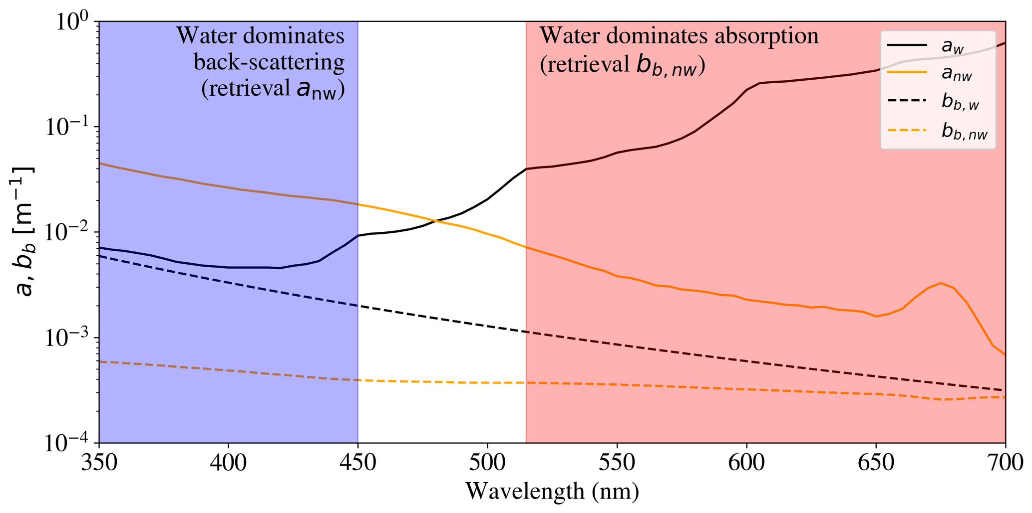
Figure 1 Comparison of the IOP spectra for water ($a_{\mathrm{w}},b_{\mathrm{b},\mathrm{w}}$; solid and dashed black curves) versus one example set of non-water spectra ($a_{\mathrm{nw}},b_{\mathrm{b},p}$; solid and dashed orange curves) from L23 (their index = 170, an example representative of the open ocean with low Chl-a concentration). The red region indicates where absorption by water dominates (a_w>5a_nw). In this region, reflectance measurements constrain the non-water component of backscattering. Similarly, the blue region is where water dominates backscattering, and retrievals may constrain a_nw. In turn, for observations with noise, the inversion problem has very limited constraints on the non-water components.

As for the last point, Fig. 1 compares the absorption and backscattering coefficients of water versus one example of non-water spectra a_nw(λ), b_b,p(λ) from the L23 dataset. As emphasized in the figure, at red wavelengths a≈a_w(λ) and $b_{\mathrm{b},\mathrm{w}}\approx b_{\mathrm{b},p}$ such that the observations may constrain b_b,p. Similarly at λ<450 nm, $b_{\mathrm{b}}\approx b_{\mathrm{b},\mathrm{w}}$ and a_nw(λ)>a_w(λ) such that the observations constrain a_nw. These inferences from Fig. 1, however, rely on the strong (but frequently satisfied) prior that a_w(λ)>a_nw(λ) at λ>500 nm and $b_{\mathrm{b},\mathrm{w}}\left(\mathit{\lambda }\right)>b_{\mathrm{b},p}\left(\mathit{\lambda }\right)$ at λ<450 nm. If this is relaxed, e.g., if a_nw(λ) and b_b,p(λ) may take on any values, then the $b_{\mathrm{b}}/a$ degeneracy forces an infinite set of solutions (i.e., no unique retrieval is possible; see Sect. 3.1).

2.4 Simulating satellite observations

For many of the analyses presented here, we have generated simulated R_rs(λ) spectra for several multi-spectral and hyperspectral missions. For the fits presented in this paper, we ignore the R_rs(λ) spectra provided by L23 (generated with Hydrolight) and instead use Eqs. (8)–(10) to calculate R_rs(λ) from a(λ) and b_b(λ). We then resample these spectra to the bands/channels of several satellite missions.

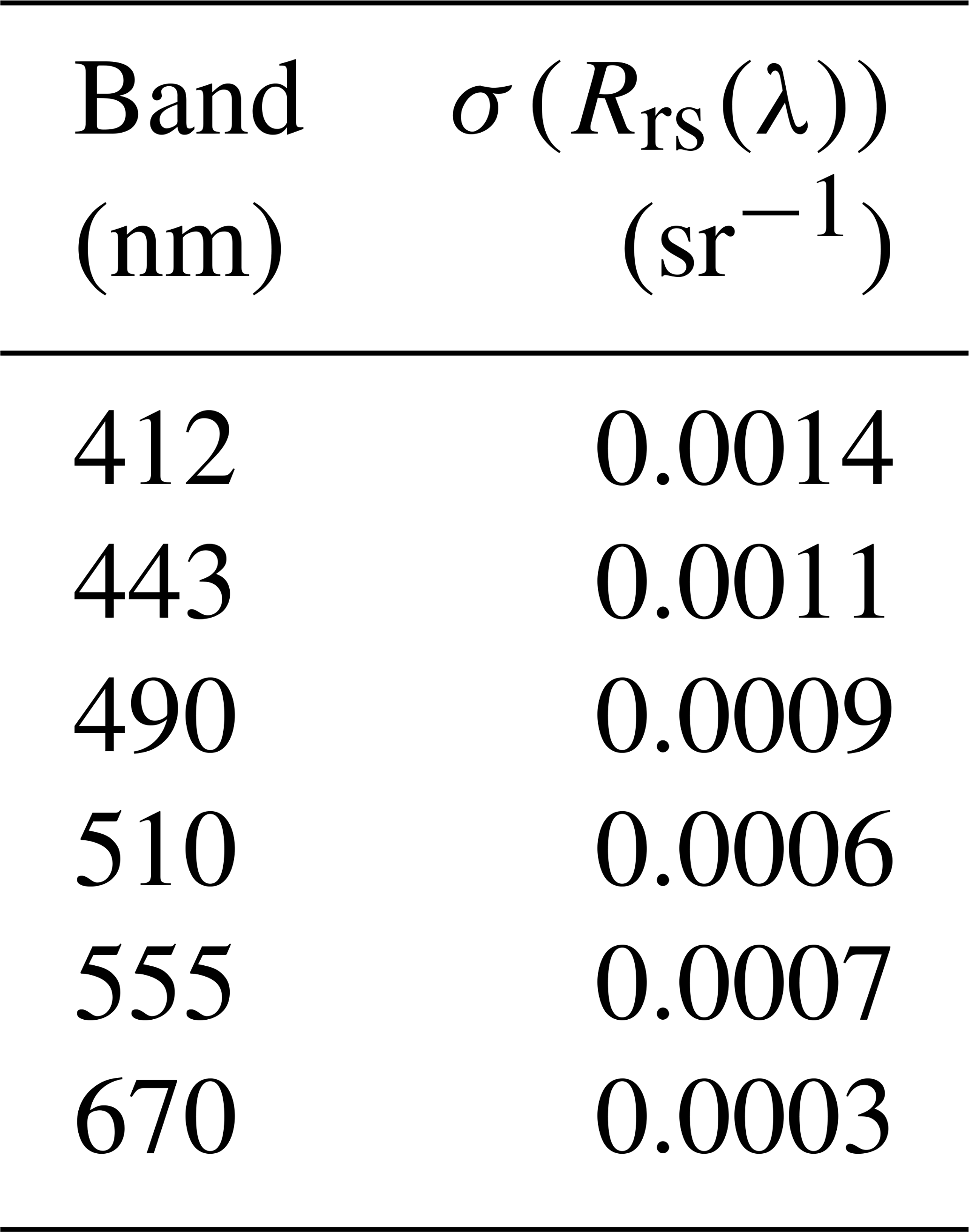
• MODerate resolution Imaging Spectroradiometer (MODIS)/Aqua. We adopt eight multi-spectral bands as listed in Table 1 corresponding to MODIS/Aqua, and we evaluate R_rs(λ) at the center of each. For uncertainties, we have estimated the RMS difference between satellite and in situ R_rs(λ) “match-up” measurements collated with the SeaBASS database (Werdell and Bailey, 2002) after iteratively clipping any 4σ outliers. Figure 2 shows an example of the data and clipping for one band. We further assumed that one-half of the variance is due to the in situ observations themselves. These RMS values are also provided in Table 1, and we find that they are in good agreement with other estimations (Zhang et al., 2022; Kudela et al., 2019).

• Sea-viewing Wide Field-of-view Sensor (SeaWiFS)/SeaStar. We followed a similar procedure for SeaWiFS using six bands and the uncertainties provided in Table 2.

• Ocean Color Instrument (OCI)/Plankton, Aerosol, Cloud, ocean Ecosystem (PACE) Satellite. For simulated OCI spectra, we assumed δ=5 nm sampling and limited the wavelength range between 400 and 700 nm. The lower bound is due to (i) greater uncertainties in the atmospheric corrections, (ii) greater uncertainty in water absorption and scattering, and (iii) greater uncertainty in how best to parameterize the non-water components in the UV bands. The upper wavelength bound is to avoid systematics that likely dominate the uncertainty at the lowest R_rs(λ) signals. Furthermore, we have limited measurements to the absorption of standard seawater constituents (e.g., phytoplankton) at these longer wavelengths.

  For the PACE noise model, we downloaded a single granule (2 175 120 pixels) of Level 2 data, v2.0: PACE_OCI.20240413T175656.L2.OC_AOP.V2_0.NRT.nc. We then took the median uncertainty spectrum (Rrs_unc; Zhang et al., 2022) for all non-flagged data between 33–40° N and 73–78° W. This median uncertainty spectrum is plotted in Fig. 3 at the Level 2 wavelength sampling (≈2.5 nm). We also show the values adopted at our δ=5 nm sampling, and one notes that we did not adjust σ(R_rs(λ)) despite the larger sampling size. This is because OCI is over-sampled at δ=2.5 nm; i.e., neighboring data points are highly correlated. Further work should assess the degree of this correlation to obtain a better noise estimate.

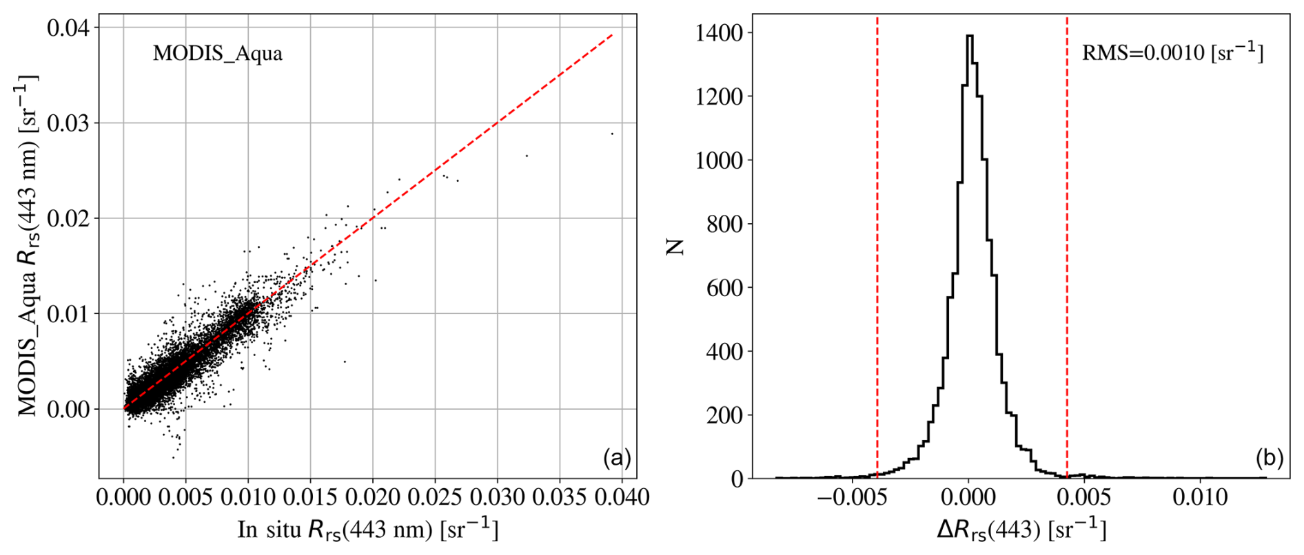
Figure 2 (a) Comparison of the MODIS measurements of R_rs(λ) at λ=443 nm versus in situ observations at the same wavelength. These were taken from the SeaBASS site (Werdell and Bailey, 2002) dedicated to MODIS matchups (NASA Goddard Space Flight Center, 2024). The points follow the over-plotted one-to-one line relatively well, albeit with significant scatter, which we assess to be the RMS noise in the MODIS observations. (b) Distribution of the difference between in situ and satellite $\mathrm{\Delta }{R}_{\mathrm{rs}}\left(\mathit{\lambda }\right)=R_{\mathrm{rs}}(\mathit{\lambda }{)}^{\mathrm{insitu}}-R_{\mathrm{rs}}(\mathit{\lambda }{)}^{\mathrm{MODIS}}$. The dashed red lines show the 4σ interval beyond which we clipped the data when calculating the noise estimate (RMS).

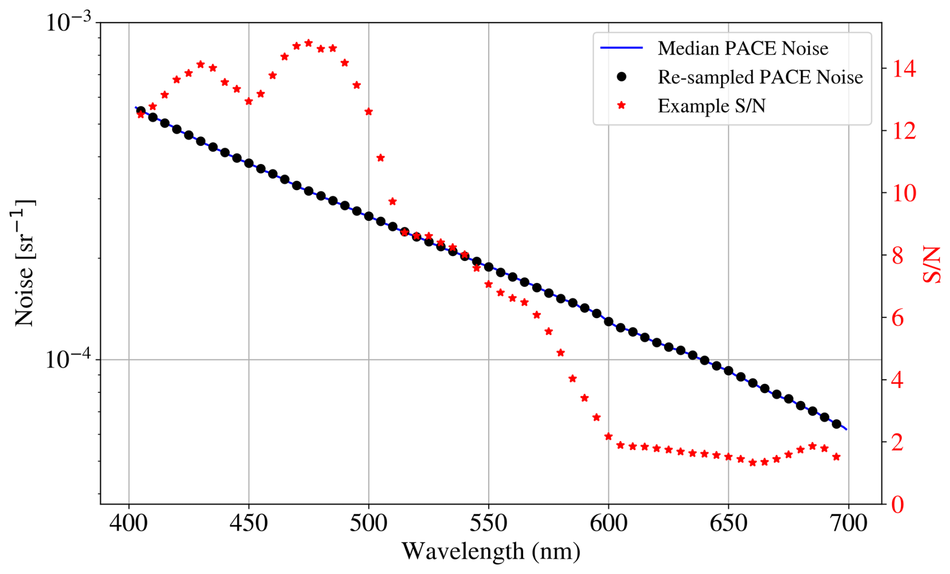
Figure 3 The blue curve is the median PACE uncertainty in R_rs(λ) estimated in the Level 2 product v2.0 for one granule (PACE_OCI.20240413T175656.L2.OC_AOP.V2_0.NRT.nc). The black dots are the values of σ(R_rs(λ)) adopted in this paper when simulating PACE spectra with noise. The red stars show the signal-to-noise (S $/$ N) ratio for an example spectrum.

Table 1 MODIS data.

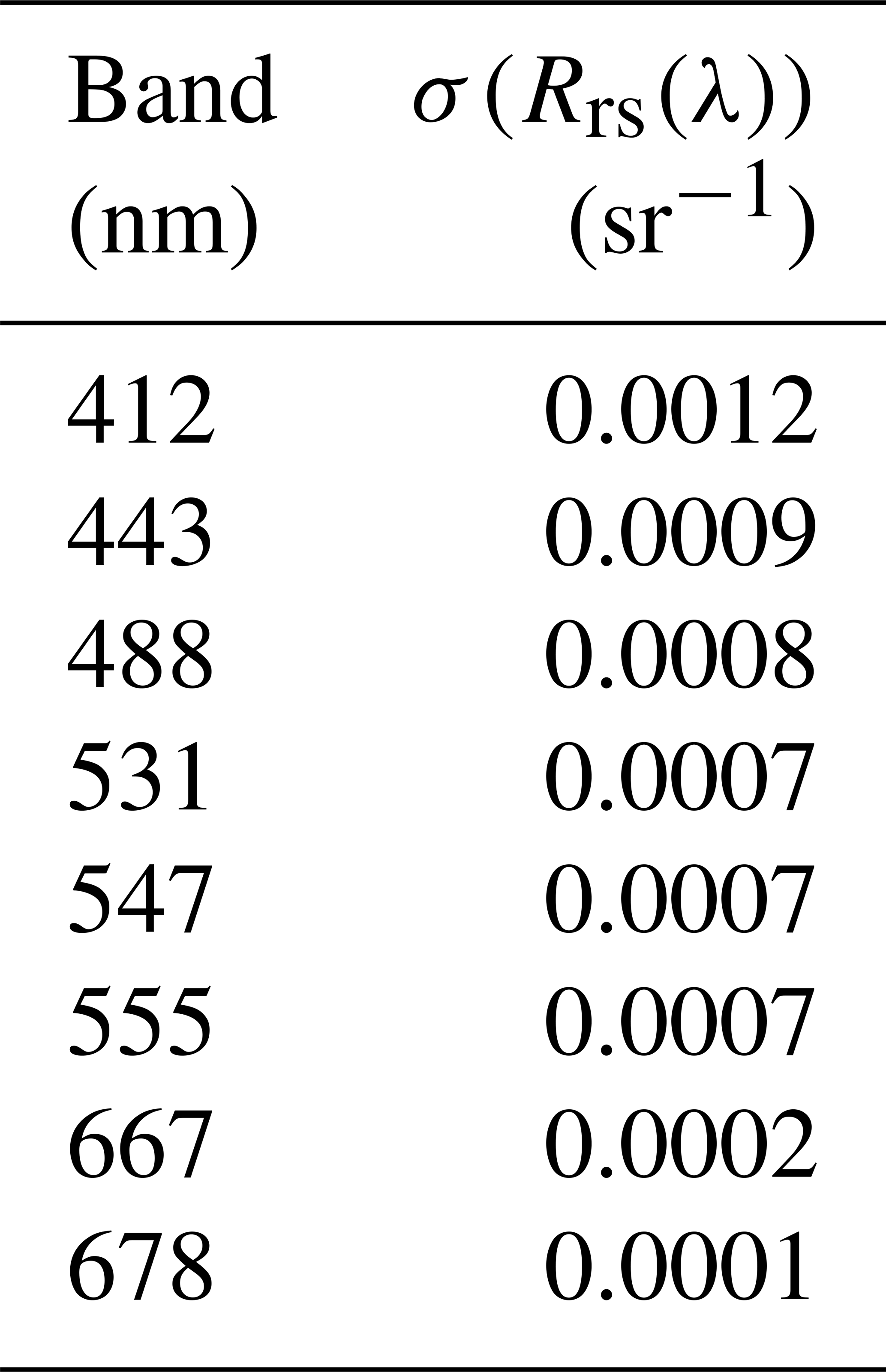
Note that the error assumes that $\mathrm{1}/\mathrm{2}$ of the variance is due to the in situ measurements.

Table 2 SeaWiFS data.

Note that the error assumes that $\mathrm{1}/\mathrm{2}$ of the variance is due to the in situ measurements.

Note that the noise is independent across spectral bands, meaning that no spectral correlation is assumed. However, in standard atmospheric correction procedures, noise is expected to be spectrally correlated due to systematic uncertainties in aerosol and Rayleigh scattering treatments, as well as instrumental effects. Ignoring these correlations could introduce additional uncertainties in the retrievals by misrepresenting the spectral structure of the observed signals. Whether treating noise as being uncorrelated maximizes or underestimates the effective retrieval uncertainty depends on the interplay between error propagation and the constraints imposed by the retrieval algorithm. A more rigorous treatment should incorporate spectral noise correlations to provide a more accurate error characterization.

2.5 IOP models

For the principal analysis of this paper, we will consider a series of increasingly complex models for the IOPs a_nw(λ) and b_b,p(λ). We generally follow common practice for models of a_nw(λ) and b_b,p(λ), which have been informed by in situ and laboratory measurements of ocean constituents. In turn, we will examine the maximum complexity that can be statistically constrained by observations designed to mimic satellite retrievals, e.g., data from multi-band and hyperspectral observations.

Consider first the simplest scenario we may conceive of: a two-parameter k=2 model with both a_nw(λ) and b_b,p(λ) taken as constant at all wavelengths.

$$\begin{array}{}\text{(12)}& {\displaystyle }{a}_{\mathrm{nw}}\left(\mathit{\lambda }\right)=A_{\mathrm{cst}}\text{(13)}& {\displaystyle }{b}_{\mathrm{b},p}\left(\mathit{\lambda }\right)=B_{\mathrm{nw}}\end{array}$$

This model may not have physical merit, but it serves as a baseline for comparison with other physically motivated IOP scenarios.

Now consider three additional models of increasing complexity. The k=3 model,

$$\begin{array}{}\text{(14)}& {\displaystyle }{a}_{\mathrm{nw}}\left(\mathit{\lambda }\right)=A_{\mathrm{dg}}\exp [-S_{\mathrm{dg}}(\mathit{\lambda }-\mathrm{400}\left)\right]\text{(15)}& {\displaystyle }{b}_{\mathrm{b},p}\left(\mathit{\lambda }\right)=B_{\mathrm{nw}},\end{array}$$

where λ is expressed in nm and where one assumes the non-water absorption is strictly an exponential function. This spectral shape is commonly used to describe the absorption by CDOM and/or detritus. In situ absorption measurements show typical values of $S_{\mathrm{dg}}\approx \mathrm{0.015}{\mathrm{nm}}^{-\mathrm{1}}$ for CDOM (Roesler et al., 1989) and $S_{\mathrm{dg}}\approx \mathrm{0.010}{\mathrm{nm}}^{-\mathrm{1}}$ for detritus (Stramski et al., 2001). Our fiducial models only require S_dg>0, but we also consider stricter priors on this parameter.

The k=4 model,

$$\begin{array}{}\text{(16)}& {\displaystyle }{a}_{\mathrm{nw}}\left(\mathit{\lambda }\right)=A_{\mathrm{dg}}\exp [-S_{\mathrm{dg}}(\mathit{\lambda }-\mathrm{400}\left)\right]\text{(17)}& {\displaystyle }{b}_{\mathrm{b},p}\left(\mathit{\lambda }\right)=B_{\mathrm{nw}}(\mathit{\lambda }/\mathrm{600}{)}^{{\mathit{\beta }}_{\mathrm{nw}}},\end{array}$$

adds the commonly adopted power law for backscattering by particulate matter (Gordon and Morel, 1983). For the k= 4 and k= 5 models, we allow β_nw to vary but consider fixed exponents for the other models introduced below (and, strictly speaking, β_nw=0 for models k= 2 and k= 3).

Last in this sequence, the k= 5 model includes a phytoplankton component:

$$\begin{array}{}\text{(18)}& {\displaystyle }{a}_{\mathrm{nw}}\left(\mathit{\lambda }\right)=A_{\mathrm{dg}}\exp [-S_{\mathrm{dg}}(\mathit{\lambda }-\mathrm{400}\left)\right]+A_{\mathrm{ph}}{a}_{\mathrm{ph}}\left(\mathit{\lambda }\right)\text{(19)}& {\displaystyle }{b}_{\mathrm{b},p}\left(\mathit{\lambda }\right)=B_{\mathrm{nw}}(\mathit{\lambda }/\mathrm{600}{)}^{{\mathit{\beta }}_{\mathrm{nw}}},\end{array}$$

with a_ph(λ) introduced to capture “typical” absorption by phytoplankton. It is expected and has been observed that this component may exhibit the greatest complexity. Indeed, scientifically, the community aims to distinguish the potentially large variations in phytoplankton families throughout the ocean and inland waters. For this k= 5 model, we adopt the parameterization of Bricaud et al. (1995):

$$\begin{array}{}\text{(20)}& a_{\mathrm{ph}}\left(\mathit{\lambda }\right)=C_{\mathrm{ph}}\left(\mathit{\lambda }\right)[\mathrm{Chl}a{]}^{E_{\mathrm{ph}}\left(\mathit{\lambda }\right)},\end{array}$$

with Chl a as the Chlorophyll-a concentration in mg m⁻³, and the tabulation of C_ph(λ) and E_ph(λ) are provided by Bricaud et al. (1998). Furthermore, we follow L23 (and the previous literature) and assume

$$\begin{array}{}\text{(21)}& \mathrm{Chl}a=a_{\mathrm{ph}}\left(\mathrm{440}\mathrm{nm}\right)/\mathrm{0.05582}{\mathrm{m}}^{-\mathrm{1}}\end{array}$$

so that phytoplankton absorption is described by one free parameter: a_ph(440 nm) (a.k.a. A_ph).

We also include a k= 2b model that has two parameters, Chl a and B_nw (we assume a constant value), and we set the A_ph using Eq. (21). This model has no CDOM or detritus absorption.

For these models, we impose the following priors (constraints) on the five parameters. For each amplitude (A_dg, A_ph, B_nw), we assume a uniform log prior from 10⁻⁶ to 10⁵ m⁻¹ in magnitude. For the shape parameters, we assume a uniform prior for S_dg in the interval $\mathcal{U}=[\mathrm{0.1},\mathrm{0.2}]$ and that β_nw has a uniform prior with values $\mathcal{U}=[\mathrm{0},\mathrm{2}]$. These priors for the shape parameters are motivated by the range of measured in situ values for each (Roesler et al., 1989; Lee et al., 2002).

We have also generated a series of “flexible” models with one free parameter at each of 61 wavelengths, and the model is the linear interpolation between each parameter. We will refer to this as the arbitrary IOP model.

For a portion of the analysis, we consider the GIOP and GSM models, which have been widely adopted within the community, including operational implementations by NASA. These two models are effectively constrained versions of the k= 5 model with different priors on the parameters. In particular, both GSM and GIOP adopt a fixed S_dg – 0.018nm⁻¹ for GIOP and 0.0206 nm⁻¹ for GSM. The models also either adopt a fixed value for β_nw (1.0337 for GSM) or estimate it from the R_rs(λ) measurements (GIOP) with a separate prescription (Lee et al., 2002).

Each model also has a different approach to setting the shape of a_ph(λ) compared to our k= 5 model. The standard GIOP model estimates Chl a from a separate prescription (typically the OC4 algorithm from O'Reilly et al. (1998) and then adopts Eq. (18) for the shape of a_ph(λ). For GSM, we adopt their multi-spectral description of a_ph(λ) and interpolate to hyperspectral resolution as needed.

We consider one final scenario, a many-parameter model (k= free) with one free parameter per wavelength channel for each a_nw(λ) and b_b,p(λ) This model is used to attempt retrievals with any arbitrary shape for the IOPs.

3 Results

3.1 Failed attempts at arbitrary IOP retrievals

The physical degeneracy in the radiative transfer relating R_rs(λ) to IOPs (Sect. 2.2) implies that the greater the freedom that one allows for a_nw(λ) or b_b,p(λ), the more degenerate the solutions. This fundamentally limits our ability to retrieve arbitrary a(λ) or b_b(λ), even in the presence of perfect data (an infinite number of channels and no uncertainty). Therefore, no algorithm can retrieve arbitrary or even highly complex a(λ) and b_b(λ). To make progress, one most also impose strong constraints on a_nw(λ) and b_b,p(λ) to recover unique or most probable solutions. These priors, however, must ensure that the values of a and b_b cannot vary freely at any individual wavelength, where one seeks a retrieval in a way that holds their ratio constant.

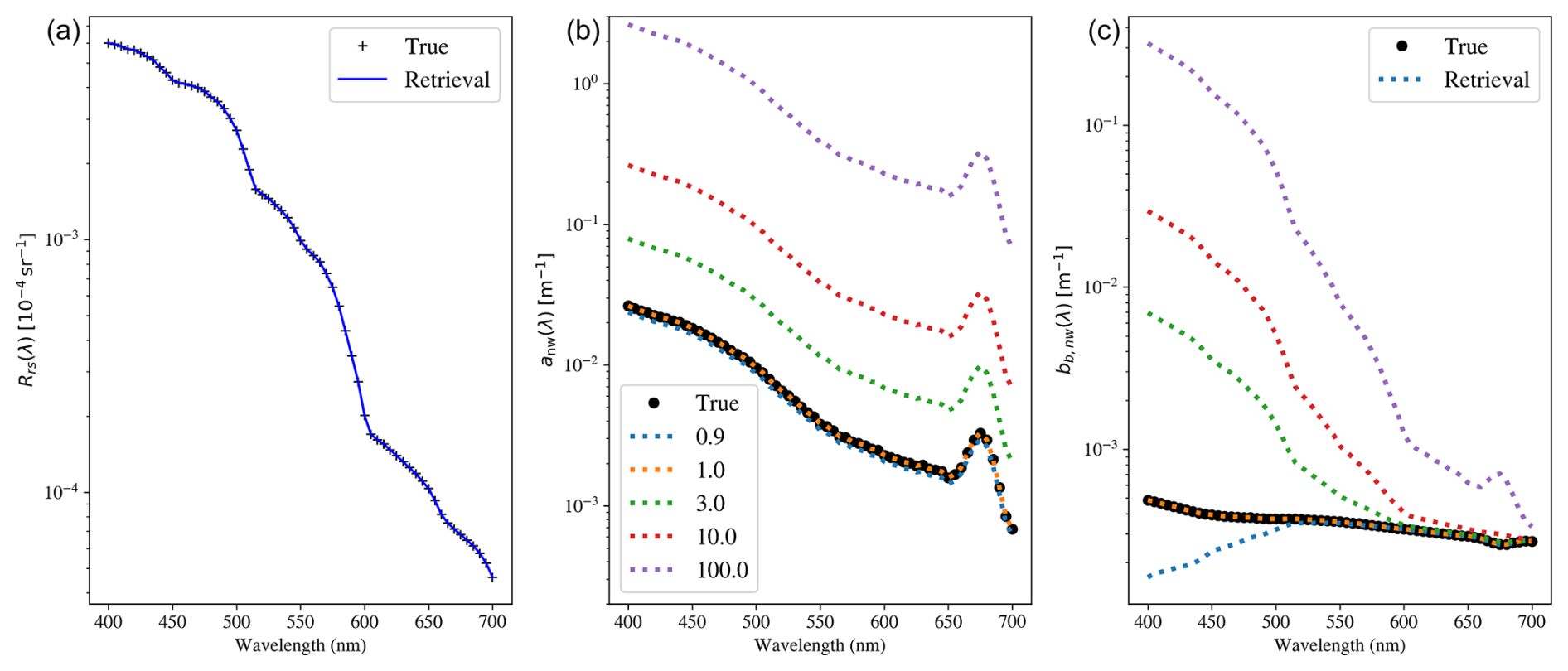
Figure 4 A series of R_rs(λ) “fits” to an example R_rs(λ) spectrum (a) for varying a_nw(λ) (b) and b_b,p(λ) (c) using the arbitrary IOP model. We show a series of solutions with scaling factors of 0.9, 1.0, 3.0, 10.0, and 100.0 relative to the true model for a(λ). Owing to the physical degeneracy in the radiative transfer equation, $R_{\mathrm{rs}}\left(\mathit{\lambda }\right)=F(a/b_{\mathrm{b}})$, there are an infinite number of such solutions, yielding infinite uncertainty in a_nw(λ) and b_b,p(λ).

To demonstrate this with an example, we performed a series of IOP retrievals of b_b,p(λ) assuming a perfect forward model (Eq. 8), perfect knowledge of the uncertainties, and perfect knowledge of water (a_w, b_b,w). In this case, we adopt the arbitrary IOP model and show the fits to R_rs(λ) for the index = 170 spectra of L23 in Fig. 4, assuming the exact answer, and then a_nw(λ) with a series of assumed scale factors. We then solved for the corresponding b_b,p(λ) spectra that provide the same best fit to R_rs(λ). Indeed, there are an infinite number of a_nw(λ), b_b,p(λ) solutions; one cannot retrieve arbitrary IOPs from R_rs(λ) spectra.

This physical degeneracy limits the information content of retrievals and precludes arbitrary functional forms for a_nw(λ) and b_b,p(λ), e.g., models that strive to retrieve arbitrary a_nw(λ) are ruled out (e.g., Loisel et al., 2018). Instead, one must impose constraints (priors) on the functional forms of a_nw(λ) and b_b,p(λ) (i.e., parameterize them) and, ideally, priors on the parameters themselves.

3.2 Parameterized IOP retrievals with BING

We now perform attempted retrievals of the IOPs a_nw(λ) and b_b,p(λ) using assumed spectral shapes with a set of increasingly complex prescriptions. We begin by fitting the k= 2 model to two examples from the L23 dataset (Fig. 5): one chosen to be representative of their full dataset and the other chosen to have a higher-than-typical phytoplankton absorption a_ph(λ) relative to the combined CDOM and detritus components a_dg(λ) (i.e., a_ph(440 nm)>a_dg(440 nm). Both have relatively low Chl-a concentrations ($\approx \mathrm{0.1}\mathrm{mg}{\mathrm{m}}^{-\mathrm{3}}$). For these, we fit to the R_rs(λ) values calculated directly from Eq. (8) and assume a constant $\mathrm{S}/\mathrm{N}=\mathrm{50}$ for the R_rs(λ) values for the likelihood calculation. Despite the extreme simplicity of this k= 2 model, the R_rs(λ) fits are not too dissimilar from the true values, especially for the high-$a_{\mathrm{ph}}\left(\mathit{\lambda }\right)/a_{\mathrm{dg}}\left(\mathit{\lambda }\right)$ example, and we note that this a_ph-dominated spectrum has a low total non-water absorption, i.e., weak a_dg absorption. This follows from our discussion in Fig. 1: water backscattering and absorption dominate the solution at short and long wavelengths, respectively, and the non-water components have limited impact on the R_rs(λ); i.e., we primarily measure seawater from IOP retrievals, especially for ocean waters with low chlorophyll concentrations.

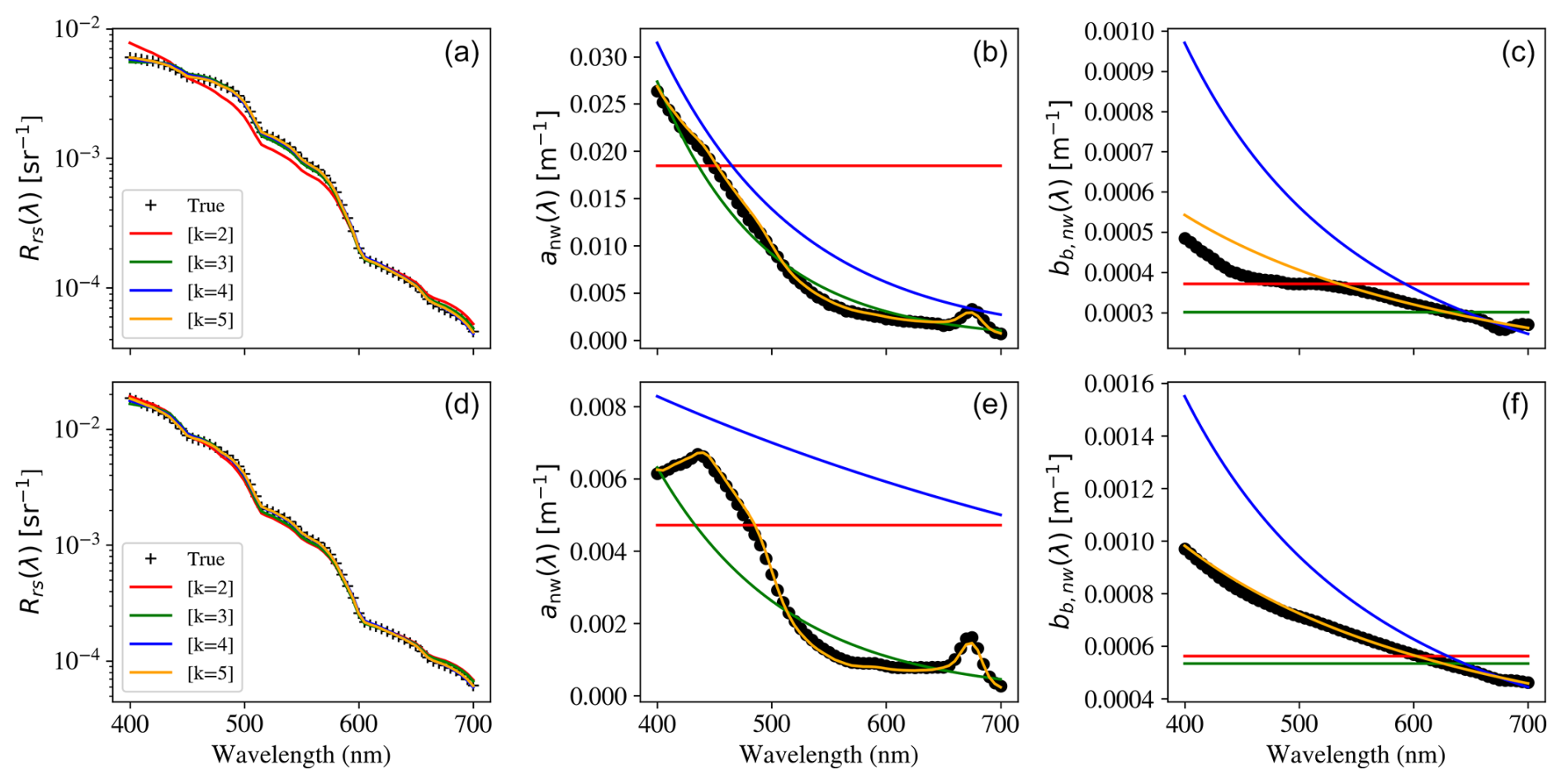
Figure 5 Retrievals of IOPs – (b, e) a_nw(λ) and (c, f) b_b,p(λ) – from fits to (a, d) remote-sensing reflectances R_rs(λ) assuming perfect radiative transfer and without adding noise. The black points are the true values of R_rs(λ), a_nw(λ), and b_b,p(λ) for two examples from the L23 dataset: index = 170, which we chose as representative of the full dataset, and index = 1032, which has a_ph>a_dg at 440 nm. The figure shows solutions for a series of models with increasing complexity and number of free parameters k. These models are (k= 2; red) constant a_nw(λ) and b_b,p(λ), (k= 3; green) constant b_b,p(λ) and a two-parameter exponential for a_nw(λ), (k= 4; blue) exponential a_nw(λ) and a power law for b_b,p(λ), and (k= 5; orange) power law b_b,p(λ) and a_nw(λ) modeled by the exponential and a phytoplankton function (see text for further details). It is evident that all of the k≥3 models produce excellent fits to the R_rs(λ) data at the few percent level.

Figure 5 shows the best solutions derived with BING for the k= 2–5 models. While the log scaling of the R_rs(λ) panels hides differences at the few percent level, it emphasizes that distinguishing between models requires nearly perfect observations. Notably, when k=2, the model does not fit the observed a_nw(λ) and b_b,p(λ) well, suggesting that this level of complexity is insufficient to fully capture the IOP variability. However, despite these discrepancies in IOPs, the R_rs(λ) fit remains relatively good, which indicates that multiple IOP configurations can produce similar reflectance spectra due to the underlying ill-posed nature of the inversion problem. As model complexity increases, the R_rs(λ) fit improves. k= 3 reproduces the reflectance spectrum to within 10 % at all wavelengths, and the k= 4 and k= 5 models achieve even better agreement, at the several percent level or less. The k= 4 model achieves a reduced chi-squared ${\mathit{\chi }}_{\mathit{\nu }}^{\mathrm{2}}\approx \mathrm{1}$ when assuming 5 % uncertainties (S $/$ N = 20) in R_rs(λ), suggesting that the model complexity is well-matched to the information content in the data. We have also considered the k= 2b model (not shown) but find that because it does not capture the exponential-like absorption of CDOM and detritus, it is generally a poorer model.

This progression implies that increasing k improves retrieval fidelity up to a certain point. If k=5 continues this trend, one might expect a reasonably good retrieval of a_nw(λ) and b_b,p(λ) under ideal conditions. However, Fig. 5 also underscores a fundamental limitation in IOP retrievals: beyond a certain level of complexity, additional parameters may not significantly enhance the retrieval unless supported by sufficiently independent spectral information. This illustrates the inherent degeneracy in the inversion problem, where different IOP parameterizations can yield similar R_rs(λ), making it difficult to extract unique IOP solutions. Thus, while a k= 5 model might provide a better fit, it remains constrained by the amount of independent spectral information available in the data, reinforcing the challenge of retrieving detailed IOP spectra from multi-spectral or even hyperspectral observations.

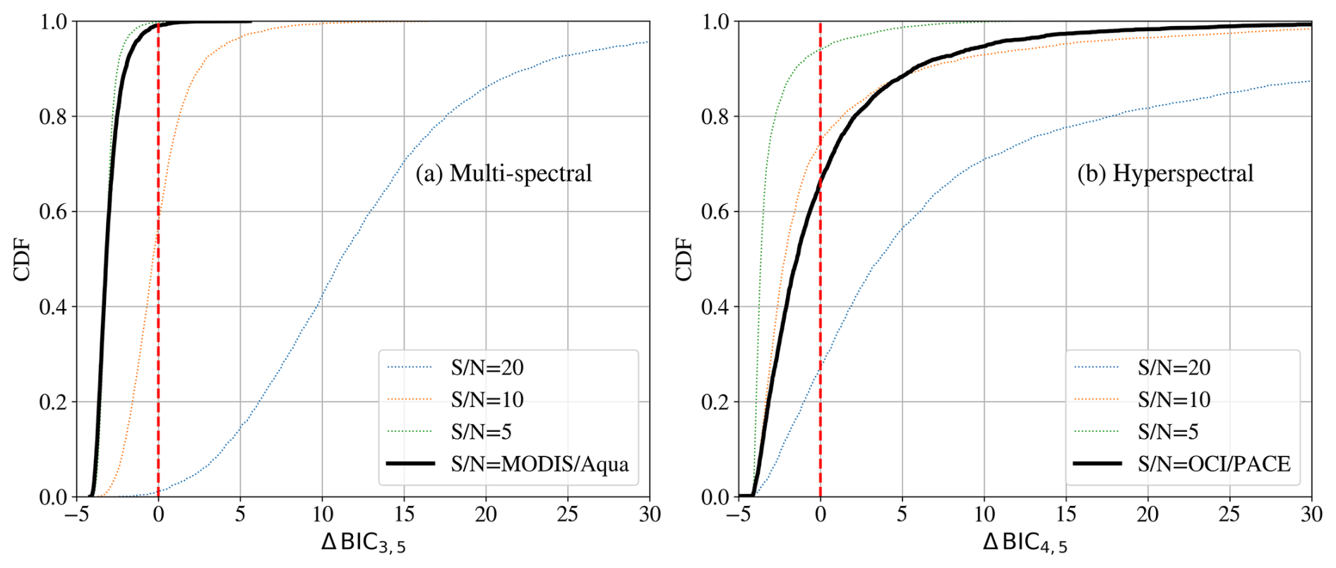
Figure 6 Evaluations of the difference in BIC values, ΔBIC, for fits to reflectance data derived from the 3320 spectra of L23. The curves describe the cumulative distribution function of the ΔBIC values. (a) Simulated MODIS observations (eight bands) with a series of signal-to-noise (S $/$ N) assumptions (colored curves) and for retrievals adopting actual MODIS noise estimates from NASA validation (Werdell and Bailey, 2002). The > 99 % negative ΔBIC_3,5 values for the realistic noise case indicate that the L23 spectra greatly favor models with only three parameters and without phytoplankton. (b) Similar analysis but for OCI-/PACE-simulated observations with fixed S $/$ N and for a best guess at nominal OCI/PACE performance (Sect. 2.3). We find, even with OCI, that only ≈30 % of the L23 dataset favors the model with phytoplankton.

We can statistically evaluate the constraining power of the data with the BIC formalism introduced in Sect. 2.1. Figure 6 shows the ΔBIC values for simulated MODIS observations of the L23 spectra (see Sect. 2.3 for details). The cumulative distribution function (CDF) on the y axis represents the cumulative probability that the ΔBIC values (Eq. 7) for the 3320 fits to the L23 R_rs(λ) data are less than or equal to a specific value. Each ΔBIC value corresponds to a comparison between two models, specifically the BIC values for a model with and without phytoplankton parameters (k= 3 and k= 5 in the multi-spectral case (Fig. 6a) and k= 4 and k= 5 in the hyper-spectral case (Fig. 6b)). If the CDF value is y_CDF at a specific ΔBIC value, it means that the 100×y_CDF % of the ΔBIC values in the dataset are less than or equal to that specific value. Thus, the CDF curve shows the proportion of the dataset for which the simpler model is preferred as a function of the ΔBIC value. The higher the CDF value at ΔBIC=0, the higher the fraction of the dataset that favors the simpler model over the more complex one.

For the analysis with a realistic MODIS noise model, fewer than 1 % of the spectra prefer the k= 5 model with phytoplankton. This holds true even though our analysis assumed a perfect forward model and perfect knowledge of the measurement uncertainties, without correlated errors. Allowing for these uncertainties would result in zero cases with ΔBIC<0. In fact, we find that one cannot retrieve more than three parameters from MODIS observations and that even the k= 2 model is satisfactory for low-Chl-a waters (Appendix B). Without perfect knowledge of the absorption by CDOM, one cannot retrieve phytoplankton from MODIS observations alone.

The curve corresponding to $\mathrm{S}/\mathrm{N}=\mathrm{20}$ in Fig. 6a shows that while there is some support for the simpler model, indicated by the CDF values for positive ΔBIC, the more complex model, which includes additional parameters for phytoplankton, is generally preferred. This is because the CDF for negative ΔBIC values is low, indicating that the simpler model is not favored in most of the dataset. In other words, although the simpler model is supported in some cases, the overall trend indicates that the more complex model is usually favored for $\mathrm{S}/\mathrm{N}=\mathrm{20}$. Thus, reducing noise in the R_rs(λ) data is essential when increasing model complexity. However, achieving $\mathrm{S}/\mathrm{N}=\mathrm{20}$ is challenging, even at blue wavelengths in open-ocean Case 1 waters, as demonstrated in numerous validation studies. Moreover, achieving $\mathrm{S}/\mathrm{N}=\mathrm{20}$ at λ>600 nm, where absorption by seawater alone is very high, may be impossible (Zhang et al., 2022).

We reach even stronger conclusions for simulated SeaWiFS observations that have fewer bands. Unless one identifies an approach to regularly achieve $\mathrm{S}/\mathrm{N}\gg \mathrm{10}$ measurements in the presence of all error terms (e.g., atmospheric corrections), phytoplankton cannot be retrieved from multi-spectral observations without strong additional priors. In Appendix B, we examine the GIOP and GSM models, which assume a fixed and steep S_dg shape parameter and examine the negative outcomes of this assumption. These results are central to our broader conclusion that multi-spectral satellite observations, such as from MODIS and SeaWiFS, lack the statistical power to constrain more than three parameters describing non-water absorption and backscattering. They also emphasize that retrieval performance depends on not only the number of parameters but also how they are structured within the model. Model design must account for both physical realism and statistical identifiability, especially when working with data of limited spectral resolution and a limited signal-to-noise ratio.

Now consider an assessment with simulated OCI hyperspectral observations for the PACE satellite (see Sect. 2.3 for details). Our fiducial case uses the L23 spectral sampling, and we limit the observations to $\mathrm{400}\mathrm{nm}<\mathit{\lambda }<\mathrm{700}$ nm, outside of which systematics of the L23 dataset and instrumentation dominate the uncertainties in R_rs(λ), and poor knowledge of the wavelength dependence of the ocean's constituents precludes confident analysis. Figure 6b shows the distribution of the difference in BIC values, ΔBIC, between the k= 4 and 5 models, assuming several choices for the S $/$ N ratio and our estimate for the OCI/PACE noise from v2.0 Level 2 products. We find that OCI/PACE may not recover an absorption signature of phytoplankton from water with properties similar to those represented by less than half of the L23 dataset (primarily those with lower Chl-a concentrations). We are led to conclude that one may retrieve four parameters for IOPs from an OCI-like observation and possibly a fifth. Two of these numbers describe the amplitude and shape of a_nw(λ) parameterized as an exponential, and two numbers describe b_b,p(λ) modeled as a power law. Absent strong priors that account for one of these four, extracting even one number describing a_ph(λ) (at all wavelengths) will be challenging. The following section explores such hyperspectral retrievals in greater depth.

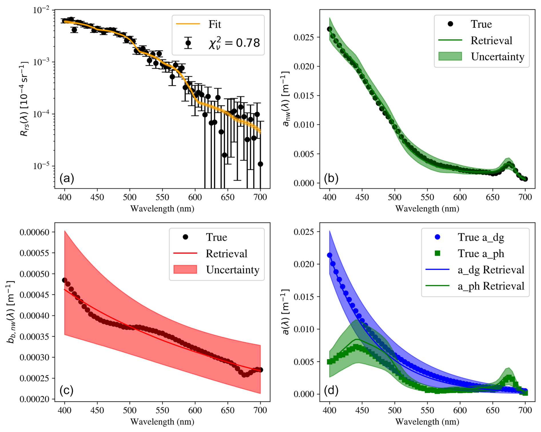
Figure 7 IOP retrievals from a BING analysis of a PACE-simulated spectrum (a) for the k= 5 model with its standard priors. For this low-Chl-a example (index = 175 of the L23 dataset), we recover estimates of a_nw(λ) and b_b,p(λ) and their uncertainties (colored curves and shaded regions that encompass the 68 % confidence intervals) that are in good agreement with the true values (solid points). However, the 99 % uncertainty interval for a_ph(440 nm) includes vanishingly small values, and we would not conclude that phytoplankton is detected at even 3σ significance.

3.3 Retrieving a_ph(λ) with NASA/PACE

The results in Fig. 6b indicate that hyperspectral observations with characteristics representative of data from the NASA/PACE mission should have the statistical power to infer the presence of phytoplankton in the majority of ocean waters. With BING, we may explore further the promise of such a_ph(λ) retrievals, as well as assess potential biases. This analysis complements the hyperspectral assessment of a portion of the NOMAD dataset of in situ observations by Erickson et al. (2023).

For the following analysis, we adopt the k= 5 model and compare results with the GIOP and GSM algorithms, re-emphasizing that the latter was only designed for multi-spectral observations and is only included for illustration. Figure 7 shows the results for the k= 5 model fit to the top spectrum in Fig. 5 but now with random noise included and with the 68 % confidence interval illustrated. The model provides an excellent description of the R_rs(λ) measurements, but the reduced ${\mathit{\chi }}_{\mathit{\nu }}^{\mathrm{2}}$ being much less than 1 suggests potential overfitting of the data. Furthermore, the retrievals are well matched to the known a_nw(λ) and b_b,p(λ) spectra and are fully encompassed by the uncertainty. This includes the individual a_dg(λ) and a_ph(λ) spectra that comprise a_nw(λ).

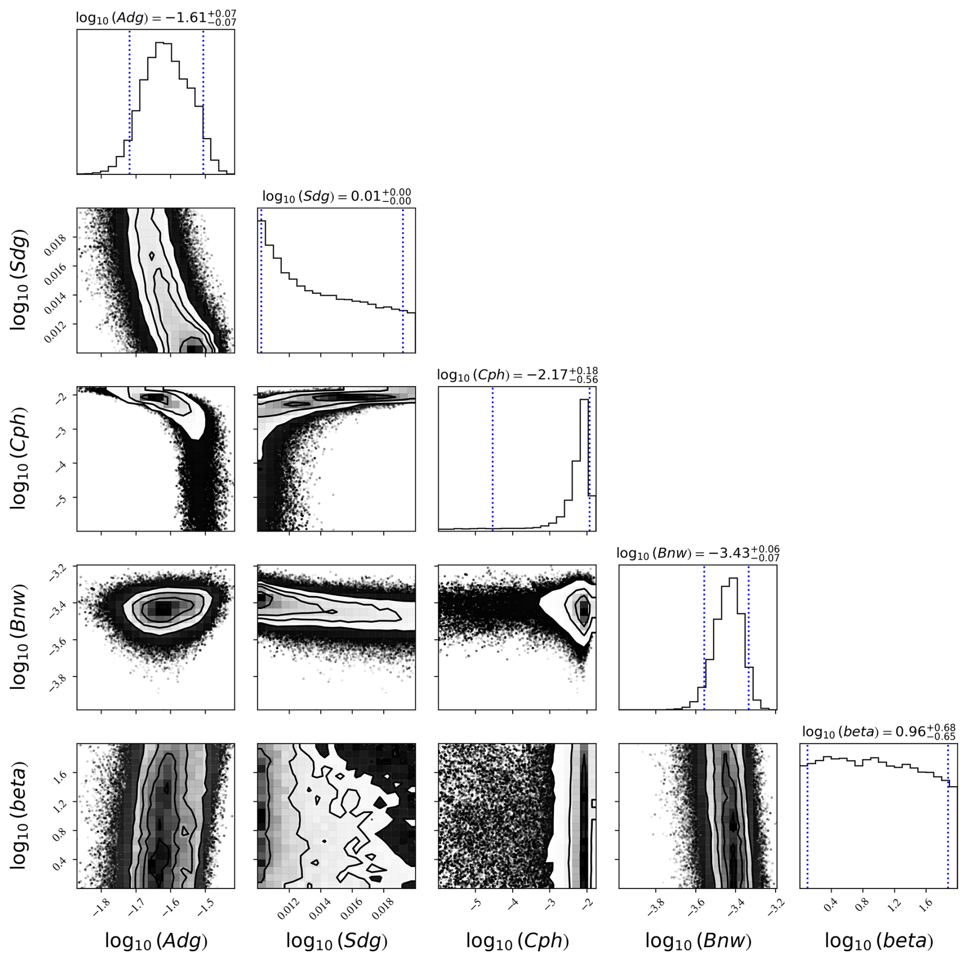
Figure 8 A corner plot showing the ≈500 000 samples of the k= 5 model fit shown in Fig. 7. The histogram panels show the marginalized posterior distributions of each parameter, with the dotted blue lines showing the 68 % confidence interval. The contour plots describe the correlations between parameters. Note especially the correlations between A_ph and both A_dg and S_dg: models with shallower S_dg and higher A_dg can describe the data without any phytoplankton absorption. Also note the very poor constraint on β_nw.

Quantitatively, on the positive side, we recover $a_{\mathrm{ph}}\left(\mathrm{440}\mathrm{nm}\right)=\mathrm{0.0084}\pm \mathrm{0.0033}{\mathrm{m}}^{-\mathrm{1}}$, which lies within 1σ of the correct value (0.0073 m⁻¹). On the negative side, the uncertainty implies less than 3σ detection; i.e., over 1 % of the MCMC samples have values 10× lower than the true a_ph(440 nm). This is due to the degeneracy between a_dg(λ) and a_ph(λ), as illustrated in Fig. 8, which shows a “corner” plot for the five-parameter model. The very low a_ph(440 nm) values ($<{\mathrm{10}}^{-\mathrm{3}}{\mathrm{m}}^{-\mathrm{1}}$) are correlated with lower (shallower) S_dg and higher A_dg, i.e., a degeneracy between CDOM/detritus and phytoplankton absorption. We also see from Fig. 8 that the R_rs(λ) offers effectively no constraint on β_nw; its values are almost entirely defined by the prior we have imposed.

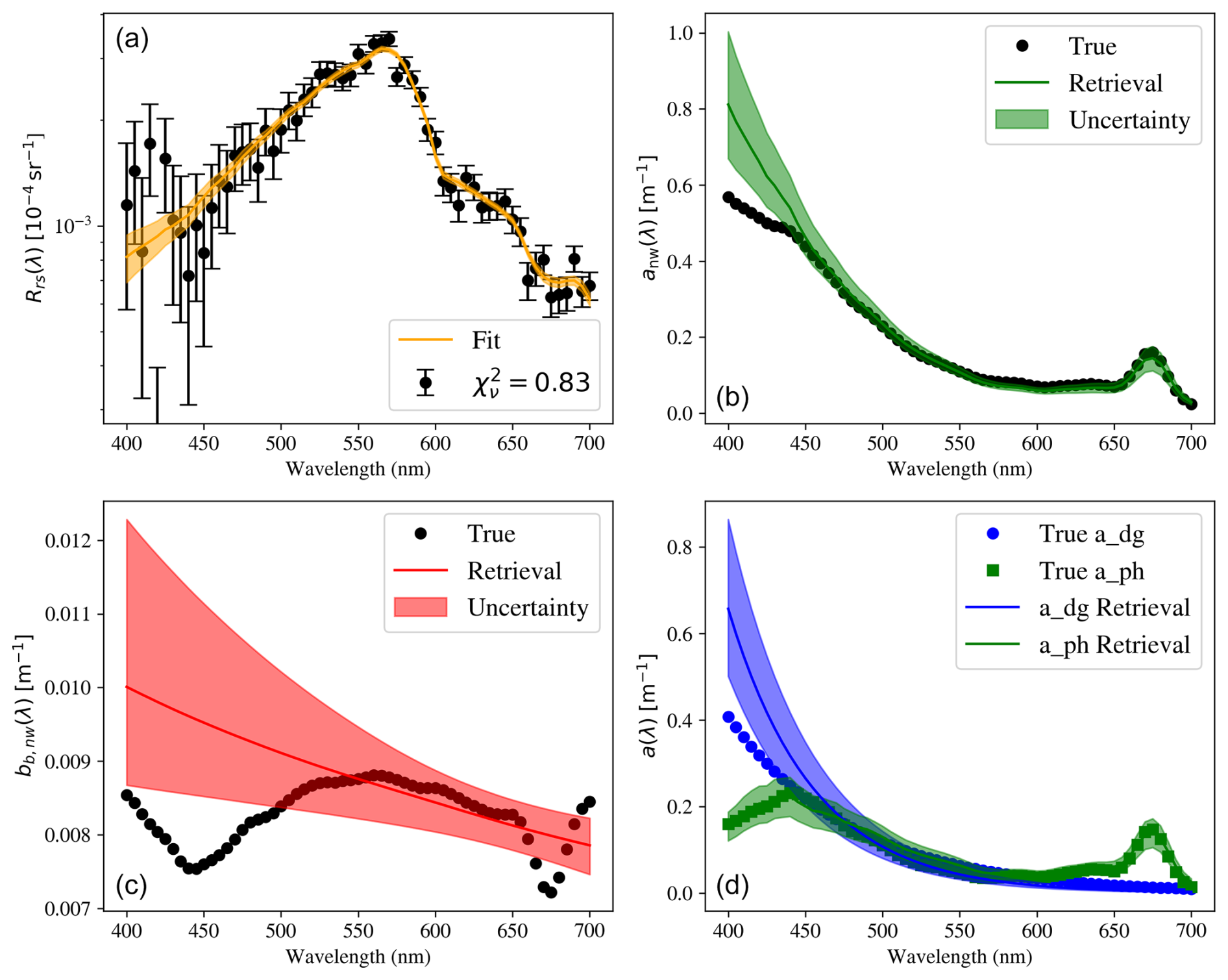
Figure 9 Similar to Fig. 7 but for an example spectrum with high Chl-a concentration and strong detrital absorption. As with the low-Chl-a case, this fit yields ${\mathit{\chi }}_{\mathit{\nu }}^{\mathrm{2}}<\mathrm{1}$ despite the overestimates of a_nw(λ) and b_b,p(λ) at λ<450 nm. This is because of the degeneracy in the radiative transfer ($b_{\mathrm{b}}/a$) and the poorer S $/$ N ratio in R_rs(λ) at these wavelengths.

Now consider an example with high Chl-a concentration. Figure 9 presents the BING fit for the k= 5 model to an example representative of eutrophic (Case II) waters (index = 2773 of the L23 dataset). The resultant R_rs(λ) spectrum shows the effects of strong detrital and phytoplankton absorption at blue wavelengths, peaking at λ≈550 nm. As with the low-Chl-a example, the a_ph(λ) and a_dg(λ) retrievals are generally in agreement with their true values, aside from an excess of a_dg(λ) absorption at the shortest wavelengths. This excess is due to the combination of a lower S $/$ N ratio in the R_rs(λ) data at λ<450 nm and errors in the adopted basis functions. In particular, our model does not capture the variations in b_b,p(λ) at λ<500 nm due to phytoplankton, and these are compensated (in part) by the higher a_dg(λ): yet another manifestation of the $b_{\mathrm{b}}/a$ degeneracy in IOP retrievals. Despite these issues, the resultant ${\mathit{\chi }}_{\mathit{\nu }}^{\mathrm{2}}$ is approximately 1 (i.e., the model fits the data well), and a more sophisticated model introduced to capture the variations in b_b,p(λ) may result in over-fitting.

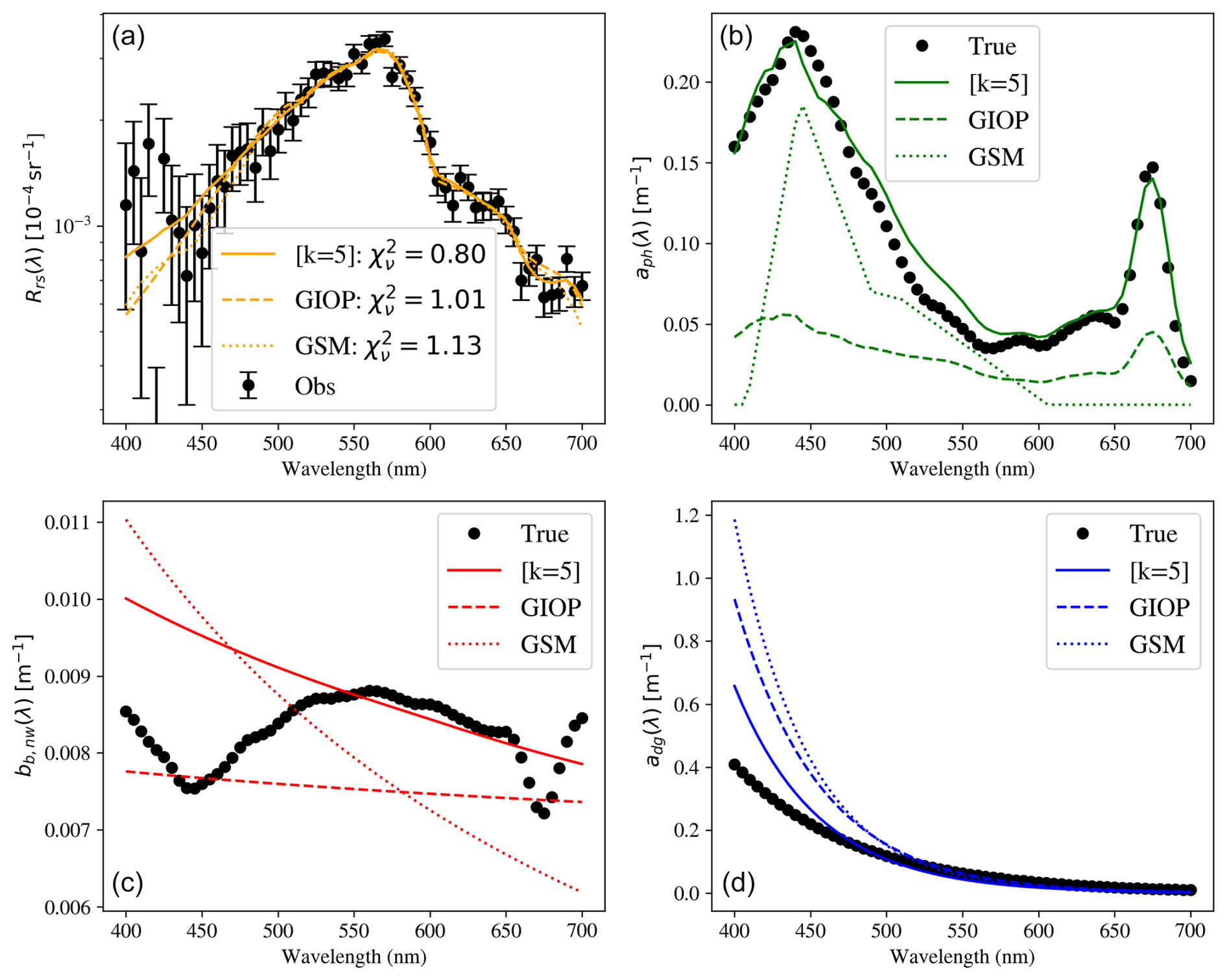
Figure 10 A series of fits and IOP retrievals for the high-Chl-a spectrum also shown in Fig. 9. The solid, dashed, and dotted curves are the results for the k= 5, GIOP, and GSM models, respectively, each with an uncertainty similar to that for the k= 5 model in Fig. 9. We find that each model provides a statistically acceptable fit to the R_rs(λ) data (${\mathit{\chi }}_{\mathit{\nu }}^{\mathrm{2}}\approx \mathrm{1}$) despite the large differences in their IOP retrievals.

We may explore the impacts of imposing priors on model parameters by comparing the fits from GIOP and GSM to this high-Chl-a example. Figure 10 shows the fits to R_rs(λ) and the IOP retrievals for these three models. All three yield a reduced ${\mathit{\chi }}_{\mathit{\nu }}^{\mathrm{2}}\approx \mathrm{1}$ and would be considered acceptable models (GSM is marginal). These results further demonstrate the physical degeneracy within the radiative transfer; here, the GIOP model systematically underestimates both a_ph(λ) and b_b,p(λ), but these compensate to yield very similar R_rs(λ) to that of the k= 5 model. We also emphasize that the GIOP model is driven to this solution by the strong prior on S_dg, the error in the estimate of Chl a from the OC4 algorithm, and the shallower slope for β_nw estimated from the Lee et al. (2002) prescription. As is obvious from Fig. 10, the best-fit a_ph(440 nm) values vary by a factor of over 400 %, much larger than the estimated uncertainties for each. These large variations occur even though the models have statistically acceptable fits. The low ${\mathit{\chi }}_{\mathit{\nu }}^{\mathrm{2}}$ values of the k= 5 and GIOP models further emphasize that the data have limited statistical power to retrieve any additional constraints on phytoplankton beyond what is described in the Bricaud et al. (1998) prescription. While different retrieval models yield substantially different estimates of a_ph(440 nm), the spectral information in R_rs(λ) alone is insufficient to independently resolve phytoplankton absorption without relying on empirical parameterizations. This points to the need for additional observational constraints, such as hyperspectral measurements, to break the degeneracy and improve the accuracy of phytoplankton absorption retrievals.

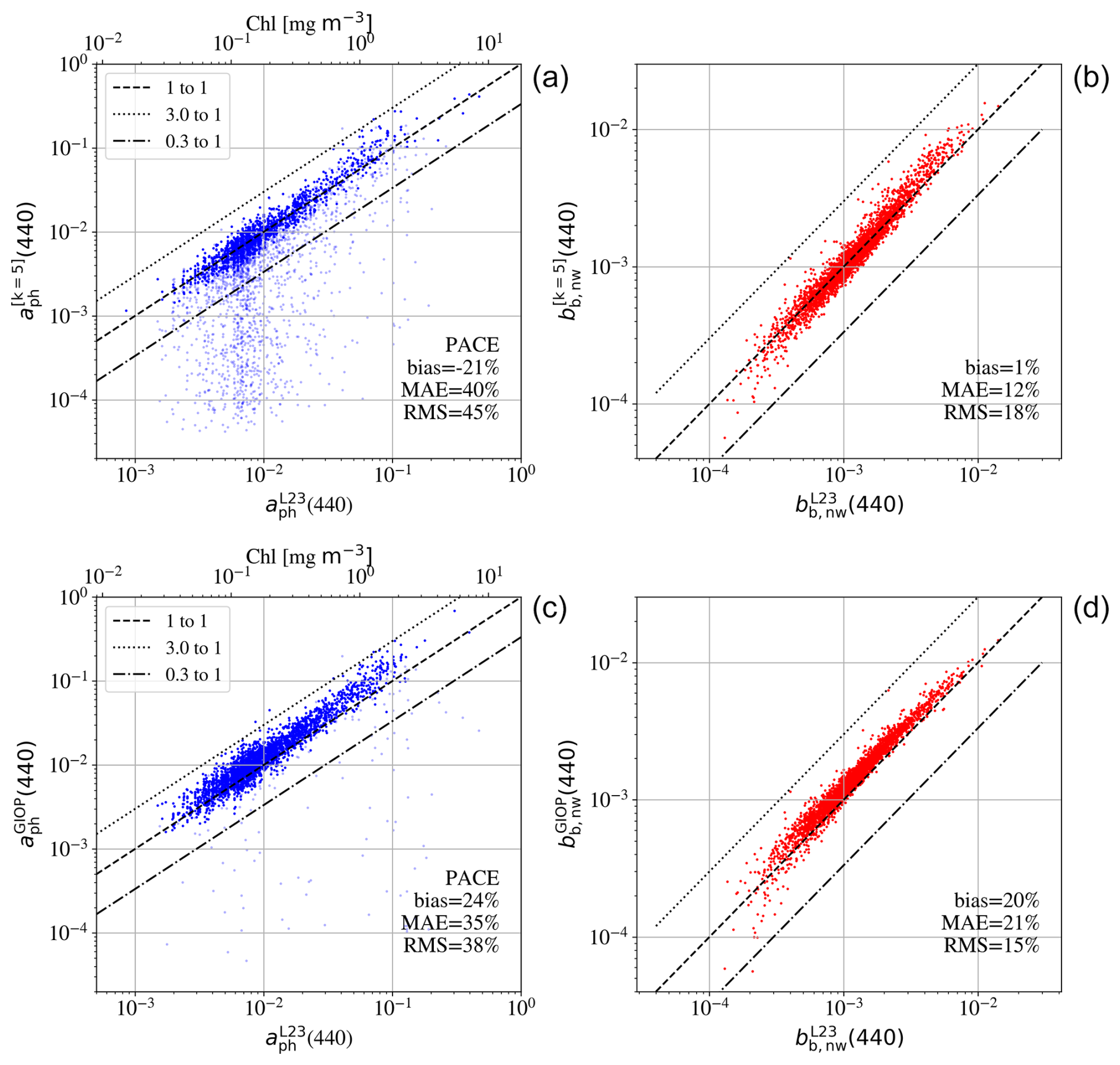
Figure 11 Panels (a) and (c) show the retrievals of a_ph(440 nm) for simulated PACE spectra versus the true values for the k= 5 (a, b) and GIOP models (c, d) using the BING package. When the error in a_ph(440 nm) exceeds 3 times the best value, we plot the measurement in light blue. The dashed curve is the 1:1 line. The right panels show the retrievals for the particulate backscattering at 440 nm. The bias, median absolute error (MAE), and root mean square (RMS) are indicated in each panel.

We have performed BING fits with the k= 5 and GIOP models to simulated PACE spectra for the full L23 dataset to estimate a_ph(440 nm) and b_b,p(440). As above, we limit the range to 400–700 nm, adopt the PACE uncertainties (Fig. 3), and have injected random noise into each spectrum. Figure 11 compares the a_ph(440 nm) and b_b,p(440) retrievals with BING versus the true values. For a_ph(440 nm), on the positive side, the retrievals track the known values over nearly 3 orders of magnitude. At low a_ph(440 nm), however, the k= 5 model systematically underpredicts a_ph(440 nm) for many of the retrievals, leading to a negative bias, and the majority of these are formally upper limits (plotted in a lighter shade of blue). Furthermore, the scatter is higher than the PACE Level 2 requirements (35 %; Cetinić et al., 2018). If we limit to cases with true $a_{\mathrm{ph}}\left(\mathrm{440}\mathrm{nm}\right)>\mathrm{0.01}{\mathrm{m}}^{-\mathrm{1}}$, the bias is reduced (15 %), but the MAE remains large (40 %). One of the primary reasons the k= 5 model underestimates low a_ph(440 nm) values is the spectral degeneracy between a_ph(λ) and a_dg(λ). When a_ph(440 nm) is weak, the total absorption is largely dominated by CDOM, making it difficult to separate the phytoplankton contribution from the background absorption (Houskeeper and Hooker, 2025). The k= 5 model allows for flexibility in the spectral shape of a_dg(λ), which can lead to overestimation of CDOM/detritus absorption and a corresponding underestimation of phytoplankton absorption.

The GIOP model, in contrast, constrains CDOM absorption using a fixed spectral slope (S_dg) that is typically prescribed from empirical studies such as Lee et al. (2002). This constraint prevents the retrieval from assigning excess absorption to a_dg(λ) at short wavelengths, reducing the risk of underestimating a_ph(440 nm). While this approach limits retrieval flexibility, it also helps stabilize the separation between phytoplankton and CDOM absorption, ensuring that even at low a_ph(λ) values, the retrieval does not shift excessive absorption to CDOM. The right panels of Fig. 11 show the retrievals for b_b,p(440). The k= 5 model provides better overall agreement with the true values, although some scatter persists, particularly at low b_b,p(440) values. The bias and MAE are smaller compared to the GIOP results, suggesting that the additional flexibility in the k= 5 model helps capture variations in backscattering more accurately. In contrast, the GIOP retrievals exhibit a consistent bias in b_b,p(440). This can be attributed to the model's prescribed functional form for backscattering, which lacks flexibility when representing natural variations in b_b,p(440) across different water types. The constrained power law exponent used in GIOP may not accurately reflect regional or case-specific spectral slopes, leading to systematic errors. As a result, while GIOP provides a reasonable fit to R_rs(λ), its retrieved b_b,p(440) values tend to be biased relative to the true values, particularly in optically complex waters.

To improve the Bayesian approach and reduce the underestimation of a_ph(440 nm) at low values, one may consider refining prior constraints on CDOM absorption, incorporating additional spectral information, and enhancing regularization techniques. Strengthening Bayesian priors on the CDOM spectral slope (S_dg) based on climatologies or independent datasets can help prevent over-attribution of absorption to CDOM. Incorporating near-UV bands (350–400 nm), where CDOM absorption dominates, provides an additional constraint to improve separation from phytoplankton absorption. Enhancing Bayesian regularization with priors that favor realistic a_ph(λ) spectral shapes and implementing adaptive noise weighting can help mitigate retrieval biases in low-absorption regimes. Finally, performing ensemble retrievals, where multiple runs with varied priors are averaged, can further stabilize the retrieval versus noise. These refinements will improve retrieval accuracy and reduce systematic underestimation of a_ph(440 nm) in low-chlorophyll waters.

4 Discussion and future prospects

In this paper, we have introduced BING, a Bayesian inference algorithm for IOP retrievals utilizing the Gordon coefficients for radiative transfer. We have reemphasized a known but underappreciated physical degeneracy in the radiative transfer – r_rs(λ) as a function of $b_{\mathrm{b}}/a$ – which strictly limits one's ability to retrieve a(λ) and b_b(λ) without strong priors. Two of the priors are natural: water both absorbs and scatters light with precisely known coefficients, at least for wavelengths λ>400 nm. We demonstrated, however, that even these constraints are insufficient; indeed, water frequently dominates the model, limiting the extraction of additional information. Consequently, we found that multi-spectral observations with published uncertainties (Zhang et al., 2022) cannot reliably retrieve phytoplankton absorption and that even hyperspectral observations (e.g., OCI/PACE) will be challenged (Fig. 6).

Previously, Cael et al. (2023) reached a similar inference as one of our primary conclusions – the limited information content of remote-sensing observations. Specifically, they analyzed the degrees of freedom (DoFs) of R_rs(λ) data through a standard principal component analysis, finding that in situ R_rs(λ) data with MODIS sampling has only 3 DoFs and inferred only DoF=2 for remotely sensed R_rs(λ). Our analysis, which includes several constraints such as water absorption and scattering, yields at least one additional parameter, but the overarching implication is similar: retrievals from R_rs(λ) observations have limited information content.

On statistical grounds, retrieving a_ph(λ) from R_rs(λ) is fundamentally challenging because CDOM and detrital absorption, which are always present, exhibit strong spectral overlap with phytoplankton absorption in the blue region. In fact, this component (a_dg) tends to exceed a_ph, even in the open ocean (Siegel et al., 2013; Hooker et al., 2020; Houskeeper and Hooker, 2025). When a_dg(λ) is parameterized as an exponential function, small variations in its spectral slope can lead to compensatory shifts in a_ph(λ), making it difficult to separate their contributions. Since R_rs(λ) depends on the combined effects of absorption and backscattering rather than direct measurement of individual IOPs, this spectral degeneracy prevents a unique retrieval of a_ph(λ) without additional constraints or priors. Previous work that published estimates of a_ph(λ) required very strict priors on the shape of S_dg (Appendix B), leading to significant bias in estimates of a_ph(λ). In the cases where S_dg was allowed to vary (Boss & Roesler, Chapter 5 Lee, 2006), the errors in a_ph(λ) were severe and limited retrievals to only upper limits, consistent with this work.

Do our results therefore invalidate the past several decades of research and data products using satellite-based ocean color observations? At the very least, all previous retrievals from R_rs(λ) must be further scrutinized. We assert that uncertainties and biases were frequently (possibly always) underestimated, and substantial correlations between retrieved parameters will be present. Unfortunately, even relative analyses of a_ph(λ) may be subject to large error. There are, however, key products that are primarily (and very nearly exclusively) empirical, i.e., generated without any radiative transfer modeling (Stramski et al., 2022). These empirically based algorithms may circumvent the radiative transfer issues raised here, but, as emphasized by Cael et al. (2023), one cannot retrieve an arbitrary number of such quantities from visible-domain R_rs(λ) observations. Therefore, the suite of products generated by the community to date are highly coupled and correlated. The limited information content of R_rs(λ) measurements subject to realistic uncertainties is inherent to the problem.

While the results from Fig. 6b indicate that hyperspectral observations offer a substantial improvement over multi-spectra data, even detecting phytoplankton remains challenging. We reemphasize that the results presented here have assumed a perfect forward model (i.e., no error in the radiative transfer calculation), uncorrelated uncertainties, a perfect model for water absorption and backscattering, and homogeneous seawater (no vertical or horizontal spatial variations). Furthermore, even if we surmount these issues, we may only be able to extract a single parameter describing phytoplankton, e.g., the a_ph amplitude at λ≈440 nm. And, strictly speaking, this may be attributed to any absorption component (not solely a_ph) that does not follow the exponential description of CDOM and detritus absorption.

Note that our findings refer to the number of statistically independent parameters that can be retrieved from ocean color reflectance data under realistic noise conditions. This does not imply that the true biogeochemical variables in nature are independent. On the contrary, many of the optical components, such as phytoplankton absorption and backscattering, are physically coupled. For example, phytoplankton both absorb and scatter light, and their associated IOPs are often correlated through cell size, composition, and pigment content. Such natural correlations are reflected in datasets like those shown in Fig. B3.

However, in an inverse problem, retrieving both components independently from reflectance requires that the reflectance spectrum contain sufficient information to statistically distinguish them. The BIC and MCMC approaches quantify how many distinct degrees of freedom are supported by the measurements and not how many physically or biologically separate variables exist, which in turn determines the number of parameters that can be reliably estimated in models of a(λ) and b_b(λ). In situations where optical properties are highly correlated, as is often the case for a_ph(λ) and b_b,p(λ), the effective dimensionality of the solution space is reduced. This reinforces our conclusion that even when additional parameters are included in the forward model, they are not necessarily identifiable unless the reflectance data provide enough information to constrain them independently. Incorporating prior knowledge about natural covariation between variables is one promising strategy to improve retrievals. Future work should explore how physically informed priors can be integrated into the inversion framework without artificially inflating confidence in individual parameter estimates.

5 Conclusions

The ocean color remote-sensing community faces a fundamental challenge in retrieving IOPs from remote-sensing reflectance due to a physical degeneracy in the radiative transfer equation. Our analysis demonstrates that this degeneracy severely limits the number of parameters that can be reliably extracted from R_rs(λ) observations. For multi-spectral satellite data with realistic noise levels (e.g., MODIS, SeaWiFS), we find that only three parameters can be reliably constrained, which is insufficient to independently retrieve phytoplankton absorption without strong, potentially biasing priors on the spectral shape of CDOM/detritus absorption. Even with hyperspectral observations like those from OCI/PACE, retrievals remain limited to four or five parameters at most, and the detection of phytoplankton absorption is still challenging in many oceanic conditions. In essence, this sets a limit on the information content available in ocean color observations (Cael et al., 2023).

These findings suggest that previous IOP retrieval algorithms likely underestimated uncertainties and may have introduced systematic biases into their estimates of phytoplankton absorption. The widespread practice of fixing the spectral slope of CDOM/detritus absorption (S_dg) to a steep value in models like GSM and GIOP allows for phytoplankton detection but at the cost of potentially significant biases in a_ph(λ) estimates. Our Bayesian approach explicitly incorporates priors and their uncertainties, providing a more transparent and rigorous assessment of the retrieval problem. While hyperspectral observations offer improvement over multi-spectral data, they still cannot fully overcome the fundamental limitations imposed by the physical degeneracy in the radiative transfer equation.

How might we proceed? It is abundantly clear that we must identify the optimal way to parameterize the problem to make the most effective use of the four or five parameters that describe a_nw(λ) and b_b,p(λ). For example, if we know β_nw (i.e., fix its value as a prior), we would not “waste” a free parameter to estimate its value. In short, we must harness our knowledge of the ocean from previous in situ measurements (or current, if one can afford them) to set priors on the model. These priors should be geographically and temporally variable to reflect different oceanic conditions. Because strict and biased priors have been shown to lead to inaccurate and uncertain retrievals, one must proceed cautiously. Empirically derived priors can help mitigate these issues by providing a more accurate representation of the ocean's optical properties.

One obvious community-wide effort would be to develop and agree upon strong priors for S_dg. This is current practice in many existing algorithms (e.g., GIOP or GSM, which set S_dg to a single value), but we describe the negative consequences of this extreme approach in Appendix B. Instead, we encourage the community to generate S_dg priors as probability distribution functions that vary with geographic location and time and then revisit these in our changing climate. Additionally, we must include more observations from both space and in situ measurements. From space, we must leverage the Chl-a fluorescence signal at ≈685 nm (Wolanin et al., 2015), whose production and radiative transfer are distinct from that of IOP retrievals. From the ocean, in situ observations provide invaluable validation data and may establish priors like those for S_dg. Non-visible in situ optical observations have been shown to improve retrievals of CDOM absorption and could be retained to better partition signals related to CDOM and phytoplankton biomass. Constraints on β_nw, as a function of location and season, and physical priors on the coupling of a(λ) to b_b(λ) for individual components from the physics of absorption and scattering could be impactful.

Developing community-wide Bayesian retrieval algorithms is also recommended. The ocean color remote-sensing community should be encouraged to adopt a Bayesian framework for IOP retrievals such as BING, explicitly including all priors and their uncertainties. A Bayesian approach allows for a more transparent and rigorous incorporation of prior knowledge and uncertainties, leading to more reliable retrievals. Unlike BING, however, Bayesian algorithms must adopt an accurate forward model and its uncertainties, include correlated and systematic error in the observations, and harness new data sources. We have initiated such a project – Intensities to Hydrolight Optical Properties (IHOP) – and encourage community adoption and development. The scientists focused on atmospheric corrections have already embarked on this journey, following the original insight of Frouin and Pelletier (2015).

The development of machine learning techniques for scientific exploitation is another tempting and potentially viable path to address some of the challenges presented in this paper. Optimistically, one can hope to train models that learn correlations in the R_rs(λ) spectra to predict quantities like Chl a or even signatures of phytoplankton communities (e.g., Woo Kim et al., 2022; Kramer et al., 2022). While we appreciate the potential power of such data-driven approaches, one must be mindful of the physical degeneracy of Eq. (8), which leads to very similar or even identical R_rs(λ) spectra from distinct IOPs (e.g., Fig. 10). A machine learning model cannot learn how to distinguish between these, especially in the presence of noise, nor will most industry-developed algorithms properly assess the uncertainties in such degeneracies. In practice, they would behave only according to the datasets they were trained upon; this is an implicit prior (Gray et al., 2024). Lastly, such models will not, on their own, discover new signatures of absorption in the ocean.

Increasing the spectral resolution of satellite observations can provide more detailed information about the absorption and backscattering properties of phytoplankton, thereby reducing the impact of degeneracies. Thus, the development and deployment of hyperspectral satellites with high spectral resolution across the visible and near-infrared spectrum are recommended. The recently launched PACE satellite will lead the way. Additionally, exploring alternative remote-sensing techniques, such as lidar and fluorescence-based methods, and incorporating polarization information to complement traditional ocean color observations should be considered. It is possible that inelastic processes, such as Raman scattering and chlorophyll fluorescence, will at least partially mitigate the degeneracies emphasized here by introducing spectrally distinct signals that, when accurately modeled, will provide independent constraints on phytoplankton absorption and scattering, thereby improving retrieval accuracy. These advanced techniques may provide independent measurements that help resolve ambiguities and improve the overall accuracy of phytoplankton estimates, although information gained using these new techniques should be clearly demonstrated and defined first in the field.

Several of the strategies we proposed can be practically implemented with modest adaptation of existing workflows. For instance, incorporating near-UV bands (e.g., 350–400 nm) into standard atmospheric correction and retrieval chains could significantly improve the ability to constrain CDOM absorption. Many modern sensors (such as PACE/OCI) already acquire data in this spectral region, although it is typically excluded from ocean color retrievals due to atmospheric correction uncertainties. Operational implementation would require further validation of atmospheric correction performance in the UV bands, but the gains in constraining a_dg(λ) could justify the investments in refining these procedures. UV bands could also be incorporated into empirical and semi-analytical models by extending existing parameterizations (e.g., for S_dg) and evaluating retrieval sensitivity in this region.

Refining priors on CDOM spectral slope (S_dg) can also be made operational by leveraging existing climatology and in situ datasets to generate geographically and seasonally resolved prior distributions. These priors could be implemented in a Bayesian retrieval framework as either lookup tables or probability distributions that are dynamically assigned by location and time. NASA and other agencies already maintain in situ repositories (e.g., SeaBASS), and these could support the development of such prior climatology. Incorporating them would not necessarily require a full Bayesian inversion at the operational level but could instead inform constrained retrievals with flexible priors, much like how empirical coefficients are regionally tuned in current algorithms.

Adaptive regularization techniques, which vary the strength of constraints based on the apparent information content of the input R_rs(λ) spectrum, can be integrated into operational pipelines through data-driven diagnostic metrics. For example, spectra with low S $/$ N ratios or low total absorption could trigger stronger regularization (e.g., narrower priors or more constrained parameterizations), while higher-quality spectra would allow for more flexible models. This adaptive scheme could be encoded through decision trees or lookup-based thresholding embedded in the processing architecture. Given the modular nature of existing algorithm frameworks like GIOP, such adaptive behavior could be implemented with minimal disruption.

Promoting interdisciplinary collaboration is also essential. Fostering collaboration between oceanographers, remote-sensing experts, and radiative transfer modelers to address the complex challenges of IOP retrievals can bring together diverse expertise and perspectives, leading to more innovative and effective solutions. These should include individuals with mastery of statistics, who can rigorously assess uncertainty and help develop robust and transparent algorithms.

By implementing these recommendations, the remote-sensing community can significantly enhance the accuracy and reliability of phytoplankton IOP retrievals, leading to better-informed biogeochemical models and ecological assessments. This comprehensive approach will help ensure that remote-sensing data accurately reflect the true state of the ocean's biological and chemical processes, thereby supporting more effective environmental monitoring and management efforts.

Appendix A: Scrutinizing the Taylor series expansion approximation to the radiative transfer

To examine the use of Eq. (8) as an approximation for the radiative transfer, consider Fig. A1, which plots the Hydrolight-derived R_rs(λ) of L23 converted to r_rs(λ) with Eq. (8) versus the evaluated u(λ) values using Eq. (9) at four distinct wavelengths. These evaluations follow an approximately quadratic pattern with zero y intercept. Overplotted with a dashed line is the Gordon approximation using the standard G₁, G₂ coefficients and Eq. (8). Qualitatively, the Hydrolight outputs follow the relation yet lie systematically above the curve. At its extreme, the Taylor series approximation is offset by ≈10 % at λ=370 nm and u(λ)=0.35.

To further illustrate the difference, we have fitted the G₁, G₂ coefficients to the data at select wavelengths and recover similar G₁ values but G₂ values that vary significantly with wavelength (G₂≈0.07 at λ=370 nm, $G_{\mathrm{2}}\approx -\mathrm{1.2}$ at λ=600 nm). We also find that there is significant scatter around each of the fits, with a relative RMS of ≈5 % at shorter wavelengths and of 20 % at the reddest wavelengths. We expect that this scatter is inherent to Eq. (8) and would be unavoidable if one uses this approximation, even with wavelength-dependent coefficients. An accurate retrieval algorithm would need to account for these variations or otherwise suffer from this systematic error. This is the focus of a separate algorithm that we are developing, and we also refer the readers to recent advances in approximations of the radiative transfer equation (Twardowski et al., 2018).

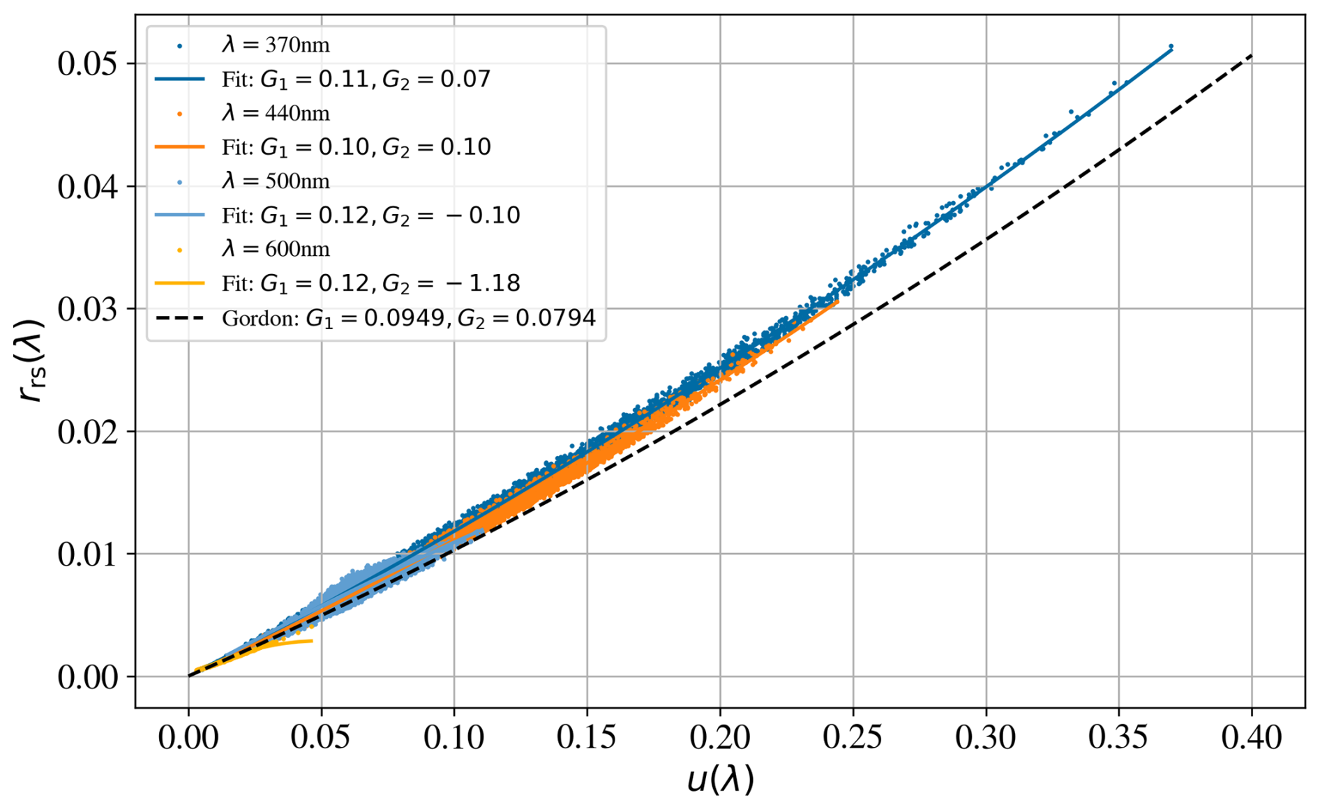
Figure A1 Sub-surface reflectances r_rs(λ) generated with the Hydrolight radiative transfer code by L23 (converted from R_rs(λ) using Eq. 10) versus u(λ) as defined by Eq. (9). The dashed black line shows the second-order Taylor expansion of r_rs(λ) in u(λ) (Eq. 8) with the Gordon coefficients that are most widely adopted by the community. In general, this curve underpredicts the r_rs(λ) calculated with Hydrolight, with a maximum offset of ≈10 % at u(λ)=0.35 and λ=370 nm. We also show a series of individual fits of Eq. (8) to the data, with the legend indicating the derived G₁,G₂ coefficients. Note that G₁ is largely independent of wavelength but that G₂ is strongly wavelength dependent (and anti-correlated).

Appendix B: Revisiting previous models

The simple IOP models examined in Sect. 3.2 resemble prescriptions adopted previously in the literature and/or implemented operationally by NASA. In light of our results, we are motivated to further examine two such models: GSM and GIOP. As described in Sect. 2.5, both GSM and GIOP adopt strict (fixed) priors on S_dg and β_nw such that these are effectively three-parameter models.

We find that by adopting these priors, these three-parameter GSM and GIOP models are statistically favored (ΔBIC>0) relative to the k= 3 model without phytoplankton for ≈50 % (GSM on SeaWiFS) or more (GIOP on MODIS) of the simulated spectra (Figs. B1 and B2). At the same time, if we relax the prior on either S_dg or B_nw, over 99 % of the spectra have ΔBIC<0 and favor the k= 3 model.

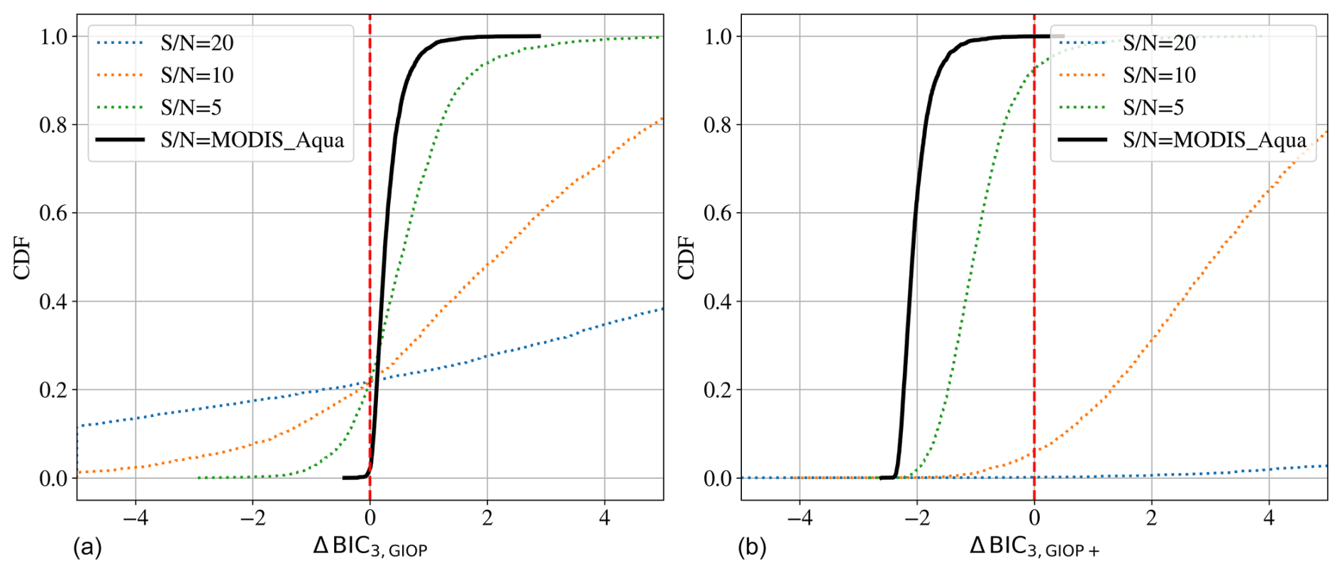
Figure B1 These panels describe the BIC analysis assuming MODIS-like observations for two models designed to match standard GIOP configurations. Panel (a) compares our k= 3 model versus the standard k= 3 parameter configuration of GIOP (see text for full details). We find that this GIOP model is preferred, which we speculate is due to the extra freedom to fit the R_rs(λ) at blue wavelengths where the S $/$ N ratio in MODIS is highest. (b) Results for the GIOP+ model (k= 4 parameters), which lets β_nw be an additional free parameter. This model is not favored for the entire dataset, further evidence that one cannot recover four parameters from MODIS observations.

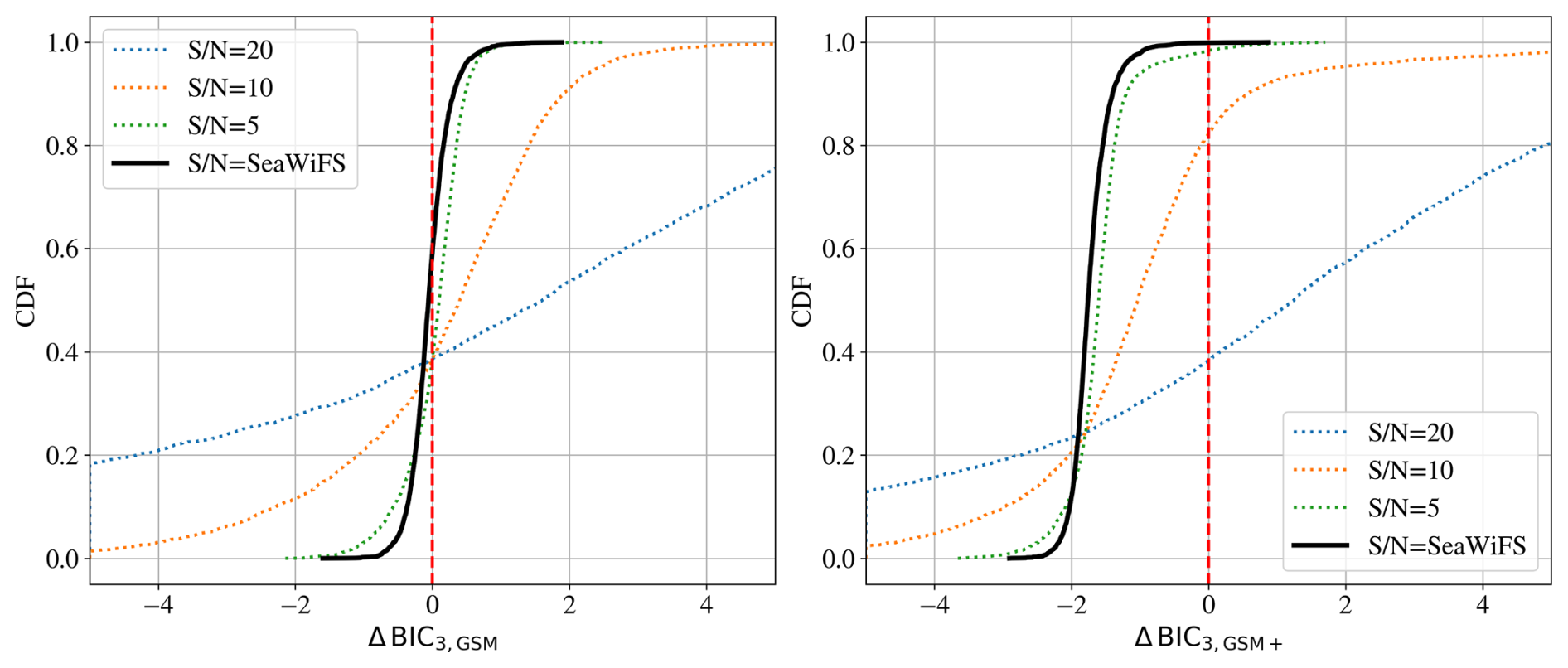
Figure B2 Similar to Fig. B1 but for GSM models and using simulated SeaWiFS spectra. As with the GIOP models, we find that the GSM model is favored over our k= 3 model but that a k= 4 parameter version – GSM+, which lets β_nw be free – is highly disfavored.

Furthermore, the fixed S_dg value adopted in each of these models is relatively steep, which imposes a significant bias on the a_ph(λ) retrievals. Let us scrutinize these priors, as they affect the potential to retrieve phytoplankton and any other constituents. Figure B3 shows the S_dg values derived with the k= 4 model (no phytoplankton) versus the fraction of non-water absorption associated with phytoplankton at 440 nm in the L23 spectra, $a_{\mathrm{ph}}/a_{\mathrm{nw}}$. The two quantities are anti-correlated because the increased presence of phytoplankton relative to CDOM and detritus tends to give a shallower non-water absorption spectrum. We find, as anticipated, that the majority of retrieved S_dg values lie within the loci of shape parameters assumed by L23 for CDOM and detritus based on Lee (2006). There is, however, a non-negligible set of retrieved S_dg values that are lower than the lowest value assumed by L23; these are partially due to strong ​​​​​​​​ ​​​​​​​​ phytoplankton absorption. Overplotted on the figure are the fixed values of S_dg for the GSM and GIOP models, where we see that their priors lie at the upper end of S_dg values measured in the ocean (GIOP) or even beyond (GSM). This was intentional for GSM (Maritorena and Siegel, 2005), as its designers derived fixed values for S_dg and β_nw by achieving the best retrievals compared to in situ data. When one adopts a relatively steep S_dg value, the absorption at λ>450 nm cannot be correctly described by CDOM/detritus, and the model will favor a higher phytoplankton contribution. If, however, the S_dg values are too steep, then one may anticipate biased a_ph(440 nm) retrievals.

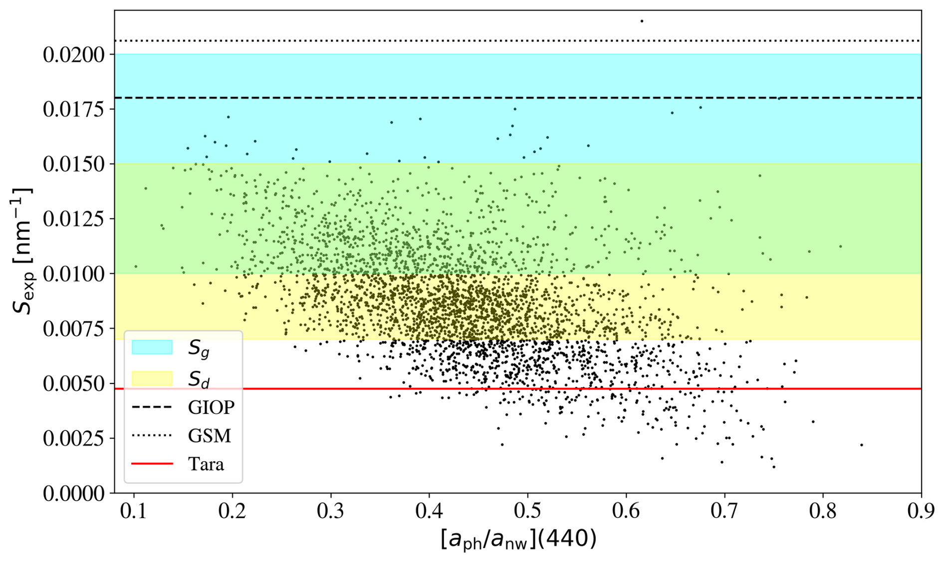
Figure B3 The dots plot the best-fit shape parameter S_dg for the L23 spectra using the k= 4 model (no phytoplankton component) versus the amplitude of a_ph to a_nw at 440 nm. The two are correlated, albeit with large scatter. The blue and yellow shaded regions indicate the ranges of exponential shapes for CDOM and detritus (S_g,S_d), respectively, adopted by L23. Not surprisingly, the majority of retrieved S_dg lie within these loci. The ones with shallower slope, however, may be attributed to the presence of phytoplankton, which effectively flattens a_nw(λ) at λ≈450 nm. The dotted/dashed black lines demarcate the fixed values of S_dg assumed by the GIOP/GSM algorithms for a_dg(λ). These are steeper values than the typical S_g (and all S_d) values adopted by L23. In addition, we show the S_dg derived from an extreme CDOM-subtracted Tara absorption spectrum collected off the coast of Africa (see Prochaska and Gray, 2024), which demonstrates at least one instance of a very low S_dg in the ocean.

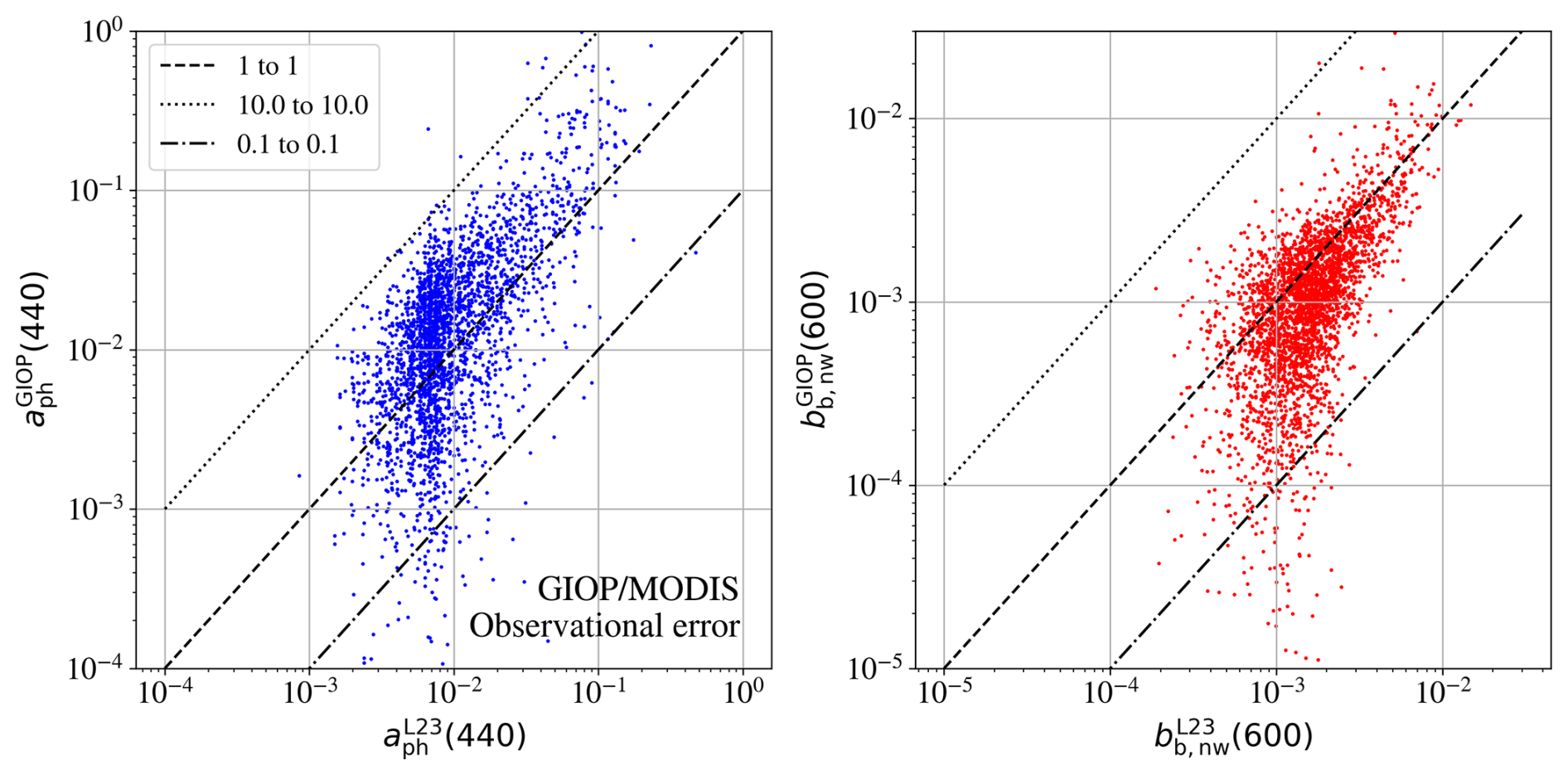
Figure B4 Retrievals of a_ph(440 nm) and b_b,p at 600 nm for the GIOP model, with simulated MODIS spectra and perturbations of the R_rs(λ) values by the typical noise. We find that the values are biased and scatter by 1 order of magnitude or more.

Figure B5 Same as Fig. B4 but for the GSM model and the simulated SeaWiFS spectra.

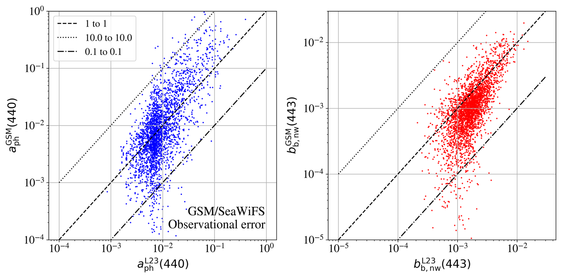
We then performed a new set of inferences on the entire L23 dataset, assuming MODIS- and SeaWiFS-simulated spectra for the GIOP and GSM models, respectively. In both cases, we calculated R_rs(λ) from Eqs. (8) and (10) and performed the inversion with the same model after perturbing the R_rs(λ) values due to the presence of noise. The retrievals are presented in Figs. B4 and B5. Clearly, the retrievals of a_ph and b_b,p are biased and highly uncertain at all values, with nearly 2 orders of magnitude of scatter. Therefore, the detection of a_ph(λ), if it were possible with multi-spectral observations, would be highly uncertain.

The constraints inherent within inversion algorithms like GSM and GIOP do affect the confidence when interpreting changes in maps of retrieved variables such as chlorophyll concentration, absorption coefficients, and backscattering coefficients. The spectral ambiguity in R_rs(λ) data can lead to changes influenced by variations in other optical properties not fully addressed by the models, making it difficult to attribute changes solely to biological factors. Moreover, the interdependence of retrieved parameters, such as chlorophyll, a_CDOM, and b_b,p, means that errors in one can propagate to others, complicating the interpretation of these maps. For example, inaccuracies in backscatter coefficient estimates can affect chlorophyll retrievals. Additionally, variability in environmental conditions can impact the accuracy of the retrieved variables. Algorithm performance may vary across different water types and regions, necessitating further caution when interpreting these changes.

Results from tests of IOP retrieval models have been presented in multiple publications over the years since the beginning of their development (e.g., Mouw et al., 2017; Werdell et al., 2018; Seegers et al., 2018), and a discussion of all of these lies beyond the scope of this paper. Nevertheless, we wish to highlight one in-depth effort summarized by the International Ocean Colour Coordinating Group (IOCCG) Report 5 (Lee, 2006). Similar to our work, the participants applied their IOP retrieval algorithms to a simulated (i.e., known) dataset to assess performance. The majority of these algorithms assumed an exponential term for CDOM/detritus absorption with fixed S_dg and a steep value ($S_{\mathrm{dg}}>\mathrm{0.015}{\mathrm{nm}}^{-\mathrm{1}}$). Similar to the results we found for GIOP and GSM (Figs. B5, B4), these consistently over-estimated a_ph(λ) at 440 nm.

Only one team (Boss and Roesler) allowed S_dg to vary (from 0.008 to 0.023 nm⁻¹) in their algorithm, which followed from the Roesler et al. (1989) publication. Referring to their Fig. 8.1, one notes less biased a_ph(λ) values than from the other algorithms and sees that they were the only group to include an error estimation. Given that the axes are a log scaling, one might miss that the uncertainties in a_ph(λ) are large enough to be consistent with zero. This implies that the retrieved values are not statistically distinguishable from zero at the given confidence level. In other words, the results from the only algorithm that allowed S_dg to vary freely indicate that a_ph(λ) could not be reliably constrained by the simulated data.