Methane ebullition as the dominant pathway for carbon sea-air exchange in coastal, shallow water habitats of the Baltic Sea

Shallow coastal marine habitats are hotspots for carbon dioxide (CO₂) and methane (CH₄) exchange with the atmosphere, yet these fluxes remain poorly quantified, limiting their integration into global and regional carbon budgets. Using floating chambers, this study quantified seasonal and annual CO₂ and CH₄ fluxes in common Baltic Sea habitats, including macroalgae-covered coarse sediments, sparsely to densely vegetated sands, submerged plant-covered mixed substrates, and reed-dominated muds. Monthly average CO₂ fluxes ranged from −937 ± 161 to 3512 ± 704 mg CO₂ m⁻² d⁻¹, with macroalgae and reed habitats exhibiting distinct flux ranges. Apart from macroalgae, all habitats exhibited a net annual CO₂ efflux. Diffusive CH₄ fluxes varied seasonally, from 0.1 ± 0.01 to 26 ± 1.5 mg CH₄ m⁻² d⁻¹, with peak emissions in summer. Ebullition occurred from March to October, reaching up to 232 mg CH₄ m⁻² d⁻¹ and contributed substantially to annual carbon-based greenhouse gas fluxes in the sand, mixed-substrate, and reed habitats. Contrary to previous findings that ebullition is confined to muddy, organic-rich sediments, this study found the highest CH₄ ebullition in vegetated sand habitats, indicating a broader spatial extent of intense CH₄ release than previously assumed. Upscaling to the shallow-water (< 6 m) zone of the Stockholm archipelago yielded total CO₂-equivalent fluxes of between −0.01 and 0.2 Tg CO₂-eq yr⁻¹ (100-year timescale). For comparison, Stockholm's energy- and transport sectors emit ∼ 1.2 Tg CO₂-eq yr⁻¹, suggesting the shallow coastal zone could be a small, but non-negligible regional source for carbon-based greenhouse gases.

1 Introduction

Coastal marine environments play a vital role in the global carbon cycle, functioning as atmospheric sources or sinks of carbon dioxide (CO₂), and as sources of methane (CH₄) (Friedlingstein et al., 2022). The sea-to-air exchange of these gases is governed by the water-air boundary layer conditions, which determine the gas transfer velocity and the gas saturation of surface waters (Liss and Slater, 1974). Coastal zones exhibit intense biogeochemical cycling fuelled by high rates of primary production, which, in combination with both terrestrial and riverine inputs of dissolved carbon species (Bauer et al., 2013), facilitates the exchange of CO₂ and CH₄ with the atmosphere (Resplandy et al., 2024).

Vascular plants and algae fix CO₂ via photosynthesis as organic material, while respiration and decomposition recycle it back to CO₂ (Gattuso et al., 1998). Dissolved CO₂ levels are also regulated by alkalinity, which affects the balance of carbonate species and is influenced by riverine input, groundwater input, sediment-seawater, and shelf-coastal exchange (Middelburg et al., 2020). In addition, CaCO₃ precipitation and dissolution can significantly modulate CO₂ dynamics in aquatic habitats (Champenois and Borges, 2021). In contrast, CH₄ in surface waters is mainly produced via methanogenesis in anaerobic, organic-rich, and sulphate-depleted sediments, and escapes via diffusion or ebullition (Reeburgh, 2007). Around 70 % of coastal CH₄ emissions are believed to come from sediment ebullition (Weber et al., 2019) which occurs when the partial pressure of the gases in the sediment exceeds their solubility at hydrostatic pressure, leading to the release of excess free gas in the form of bubbles. Due to its rapid rise rate, a large fraction of the free gas does not dissolve in the water column and hence avoids microbial oxidation before reaching the water-air boundary layer as ebullitive flux (Mao et al., 2022), adding to the diffusive exchange across the sea-air boundary (Hermans et al., 2024), particularly in shallow waters as ebullition increases with decreasing water depth (McGinnis et al., 2006). While ebullition may be the dominant flux pathway for CH₄ in coastal waters, the size of the flux remains uncertain due to its highly stochastic nature (Lohrberg et al., 2020).

There is increasing interest in using the carbon sequestration potential of the coastal ocean as a climate mitigation tool to help contain global warming as close to the 2015 Paris Agreement as possible (Claes et al., 2022). Emission reduction strategies could potentially benefit from coastal mitigation measures but require accurate quantification of emission or uptake of greenhouse gases in coastal areas. Significant uncertainties remain in the CO₂ and CH₄ budgets of coastal regions as a consequence of the scarcity of in-situ flux measurements and the difficulties of upscaling existing data due to the high spatial and temporal variability, both within and between individual habitats (Dai et al., 2022; Bange et al., 2024). Habitat-based classifications are commonly used to upscale CO₂ and CH₄ fluxes in coastal environments, particularly in well-studied systems such as mangroves, seagrass meadows, and saltmarshes, where high productivity and sediment carbon storage potential have centred most research efforts (Rosentreter et al., 2023). These classifications are often tailored to tropical and subtropical environments but may not capture the full spectrum of coastal habitat diversity, especially in northern, temperate systems.

In regions like the Baltic Sea, habitats such as macroalgal beds, mixed vascular plant communities, and sparsely vegetated sediments have been shown to exchange significant amounts of CO₂ and CH₄ with the atmosphere (e.g. Lundevall-Zara et al., 2021; Asmala and Scheinin, 2023; Roth et al., 2023). These coastal shallow-water habitats vary between annual atmospheric sources of CO₂ (Honkanen et al., 2024) and annual sinks of CO₂ (Roth et al., 2023). At the same time, recent studies indicate they exhibit CH₄ fluxes up to the same order of magnitude as mangroves (Rosentreter et al., 2018) or two orders of magnitude higher than more offshore areas of the Baltic Sea (Lundevall-Zara et al., 2021). However, the lack of a standardized, widely adopted classification system for these habitats limits the comparability and upscaling of these flux estimates. This challenge is globally further compounded by the scarcity of high-resolution coastal habitat maps (Rosentreter et al., 2023).

Only a few habitats in the Baltic Sea have observations of both CO₂ and CH₄ fluxes (Asmala and Scheinin, 2023; Roth et al., 2023), and among them almost none has a full annual coverage of flux estimates, which is crucial for the effect of the sea-air exchange on radiative forcing in the atmosphere. CH₄ has a sustained-flux global warming potential that is 45 or 96 times as efficient as CO₂ on a 100- or 20-year timescale, respectively (Neubauer and Megonigal, 2015), and as such, even relatively small mass quantities of CH₄ can significantly contribute to the net radiative forcing added to the atmosphere by the habitat (Roth et al., 2023). Since CH₄ ebullition is not included in many estimates due to the difficulties in capturing the ebullitive flux, the contribution from CH₄ is highly uncertain (Weber et al., 2019).

Various methods exist for measuring gas exchange between the water and atmosphere. These are either based on water and air concentration sampling and determination of fluxes through a gas transfer velocity parametrisation (e.g. Humborg et al., 2019; Asmala and Scheinin, 2023; Roth et al., 2022, 2023), eddy covariance (e.g. Gutiérrez-Loza et al., 2019), or floating chamber techniques (e.g. Lundevall-Zara et al., 2021), each with their own strengths and limitations (Bastviken et al., 2022). The floating chamber technique, together with the eddy-covariance method, has the benefit that the flux is determined directly, therefore avoiding the use of a gas transfer velocity parametrisation and is capable of resolving the ebullitive flux from the diffusive flux component (Iwata et al., 2018; Żygadłowska et al., 2024). However, since the floating chamber measurements have a high (analyser-dependent) sensitivity and small footprint, small-scale habitat differences can be resolved, and low fluxes can be included in habitat budgets. The floating chamber technique has been criticised for interfering with the boundary layer, inducing extra turbulence, as well as creating an environment within the chamber that is not representative for outside conditions in terms of wind, temperature and pressure (Mannich et al., 2019). However, taking caution in chamber design and use, these biases have been shown to have minor effects on the flux and for the chamber technique to produce similar flux values as other, non-interfering methods (Cole et al., 2010; Gålfalk et al., 2013; Lorke et al., 2015).

In this study, we conducted year-round floating chamber experiments in shallow (< 4 m) coastal habitats in the Stockholm and Trosa archipelagos of the northwestern Baltic Proper to quantify diffusive CO₂ and diffusive and ebullitive CH₄ fluxes. The objective was to constrain flux variability based on five habitat groups, including macroalgae-covered coarse sediments, sparsely to densely vegetated sands, submerged plant-covered mixed substrates, and reed-dominated muds. These habitats commonly occur along both the Swedish and Finnish Baltic Sea coast (Al-Hamdani and Reker, 2007). We hypothesized that CO₂ and CH₄ fluxes would vary systematically among these habitats, and that while within-habitat variability would occur, the boundaries for this variability would differ between the habitats. In this case, the habitat classification could help identify habitats that are the major contributors to the uncertainty associated with the coastal, shallow-water CO₂ and CH₄ flux. Further, the study aimed to quantify the relative contributions from CO₂ flux, diffusive CH₄ flux and CH₄ ebullition to the total CO₂-equivalent flux, identifying the dominant pathway for carbon-based greenhouse gas exchange in these habitats.

2 Methods and materials

2.1 Sampling locations and habitat classification

The sampling was carried out in seven locations in the Stockholm and Trosa archipelago seas in the north-western Baltic Proper (Figs. 1 and S1 in the Supplement). Six out of seven sampling locations were on the island of Ingarö and the seventh sampling location was on the island of Askö.

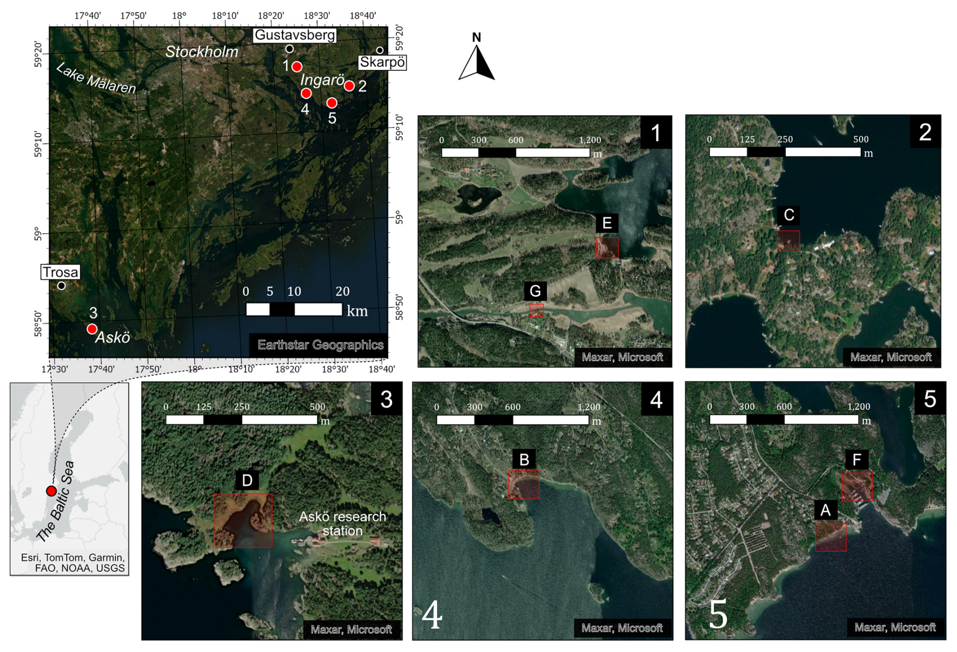
Figure 1 Map showing the sampling locations (A–G) on Ingarö and Askö. Marked out are also the weather stations in Trosa, Gustavsberg and Skarpö. Basemap imagery: Esri, TomTom, Garmin, FAO, NOAA, USGS, Earthstar Geographics, © Maxar, and © Microsoft.

The archipelagos are brackish systems where the salinity spans from close to zero in the inner archipelago near the outflow from Lake Mälaren and up to 8 ‰ in the outer archipelago (Fig. 1). The coastal biotopes consist of exposed rocky coastline, long and narrow fjord-like bays, and sheltered inlets (Hill and Wallström, 2008; Kautsky, 2008). The Stockholm archipelago is considered one of the most eutrophic archipelagos along the Swedish coastline (Hill and Wallström, 2008).

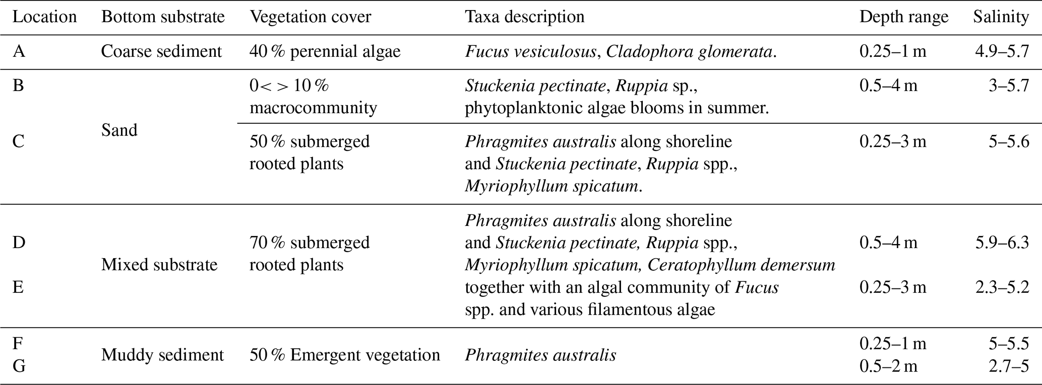
The classification scheme applied in this study is HELCOM HUB, an underwater biotope and habitat classification system developed for the Baltic Sea by HELCOM (HELCOM, 2013). The sampling locations were categorised based on bottom substrate and vegetation (Table 1). The seven sampling locations were divided into five distinct habitats: Coarse sediment with perennial algae cover (location A), sand with sparse epibenthic macrofauna community (location B), sand with submerged rooted plants (location C), mixed substrate with submerged rooted plants (locations D and E) and muddy sediment with emergent plants Phragmites australis (locations F and G). The classification was completed in September 2020. For further details on the HELCOM HUB classification and how it was carried out in the study, see Sect. S1.

Table 1 Descriptions of the sampling locations A–G as shown in Fig. 1. Descriptions of the sampling locations A–G as shown in Fig. 1. Vegetation cover refers to the average coverage in the warmer months May, June, July and September, and as an average over the whole sampled area.

2.2 Field methods

Sampling was carried out between September 2020, and October 2022, with seasonal sampling periods broadly in January (25–26 January 2021), March (27 February–2 April 2021), May (28 April–20 May 2021), June (16–17 June 2021), July (8–9 July 2021), September (14–15, 14–22 September 2022), October (26–29 October 2022), and the shift between November and December (25 November–10 December 2020).

To directly measure CH₄ and CO₂ fluxes, a floating plastic chamber was connected to an Off-Axis Integrated Cavity Output Spectroscopy (OA-ICOS) Los Gatos Research DLT-100 Greenhouse Gas Analyser (GGA). The chamber design and anchoring function is similar to those used in Schilder et al. (2016), but without an ebullition shield. The round chamber was covered with aluminium foil to reduce internal solar heating and had a volume of 7500 mL covering a surface area of 0.073 m². Foam was attached to the downward-facing sides of the chamber for flotation, and the walls submerged 1.5–2 cm into the water depending on sea state and the chamber was anchored to the seafloor. See Fig. S1a for a picture of the chamber.

The chamber was connected to the GGA via two strands of 20 m long, plastic tubing with an inner diameter of 3 mm. The tubing was connected to the inlet of the GGA via two 100 mL Winkler bottles and an Acro^® 50 vent filter to avoid particles and water droplets entering the GGA. The total volume of the chamber, tubing, Winkler bottles, filters, and cavity of the GGA was ca. 7700 mL. Air was circulated using the GGA's internal pump and sampled at a frequency of 20 s. The flux was determined from the concentration gradient during the sampling time (see section “Diffusive flux calculations”).

Each flux measurement lasted ∼ 20 min, after which the chamber was lifted from the water surface and the GGA allowed to equilibrate with the air. This short measurement time minimises bias from the effect on the flux of the increasing gas concentration within the chamber (Mannich et al., 2019). Flux measurements were conducted without compensating for potential pressure changes within the chamber as such variations have been shown to be minor (< 1 %) in light-weight floating chambers like the one used in this study (Martinsen et al., 2018). Pressure gradients of this magnitude between the ambient air and chamber environment would have a negligible effect on the flux.

At each sampling location flux measurements were typically carried out in transects from close to shore to maximum 30 m away from shore. The chamber was placed to account for variations in vegetation community and density equally and, where present, also placed over emerged vegetation. Between 3 and 76 flux measurements were done at each location, each sampling period. The sampled area per location was between 40 and 800 m².

Local wind speed, wind direction, air temperature, atmospheric pressure, and precipitation were measured during flux sampling using a Eurochron wireless weather station, ECWCC1080, mounted on a mast 1.5 m above the water surface close to the sampling location. Wind speed was adjusted to 10 m height (U₁₀) assuming a neutral logarithmic profile (Amorocho and DeVries, 1980). Equation (1):

$$\begin{array}{}\text{(1)}& U_{\mathrm{10}}={\displaystyle \frac{U_z}{\mathrm{1}-\frac{\sqrt{C_{\mathrm{10}}}}{\mathit{\kappa }}\ln \left(\frac{\mathrm{10}}{z}\right)}}\end{array}$$

where U_z is the wind speed at the measurement height (m s⁻¹), C₁₀ is the drag coefficient for shallow water (0.0013), κ is the von Kármán constant (0.4) and z is the measurement height (m). C₁₀ was chosen as the lower end of the range of 0.0013 and 0.0015 suggested by Stauffer (1980), since C₁₀ tends to decrease over shallow waters (< 3 m) and in the presence of surface films (Van Dorn, 1953; Hicks et al., 1974).

Regional timeseries of wind speed and air temperatures for the Stockholm and Trosa archipelagos were obtained from the Swedish Meteorological and Hydrological Institute (SMHI) from the weather stations in Gustavsberg, Skarpö and Trosa (Fig. 1). Wind speed was only available from Skarpö (SMHI, 2024a, b).

Water salinity and temperature were measured close to the surface (at ∼ 5 cm depth, and within 10 m of the chamber deployments) with a handheld sensor (conductivity WTW 340i).

2.3 Diffusive flux calculations

The diffusive fluxes of CO₂ and CH₄ were calculated from the change in gas concentration in the chamber-GGA system, according to Eq. (2):

$$\begin{array}{}\text{(2)}& F_{\mathrm{d}}={\displaystyle \frac{\mathrm{\Delta }C\cdot V}{A\cdot \mathrm{\Delta }t}}\end{array}$$

where F_d is the diffusive flux (mg CO₂ or CH₄ m⁻² d⁻¹), ΔC is the gas concentration change (mg L⁻¹), derived from the change in mole fraction as measured by the GGA, V is the volume of the chamber-GGA system (L), A is the chamber footprint (m²) and Δt is the duration of the measurement.

For diffusive flux measurements, the rate of concentration change measured by the GGA is expected to be near-linear. The variations in the rate of change due to changing gas transfer velocity (changes in turbulence in the boundary layer) or variations in the gas concentration during the measurement are expected to be small. This contrasts with ebullition events, which are apparent in the measured gas concentration as large, sudden changes. To exclude such events and also periods with other measurement artifacts (e.g., fitting leakage or induced turbulence from chamber deployment), we divided each measurement into five segments (each ∼ 4 min long) and performed least-squares linear regression analysis on each segment. Segments that showed an approximate linear change (R²>0.7) were used for calculating the ΔC.

For a description of the extrapolation of daily fluxes into annual fluxes, see Sect. S2 and Table S1.

2.4 Ebullitive flux

Ebullition was detected in the measurements as abrupt changes (at least three times the standard deviation of the change from the diffusive flux for a 20 s measurement interval) in concentration detected by the GGA (Fig. S2). The ebullition events either appeared as a simple, step-up in concentration, or as a peak, followed by a more gradual increase in concentration characteristic of diffusive exchange afterwards. The approach used to detect ebullition events is similar to Żygadłowska et al. (2024), and is discussed in more detail in Sect. S3.

The amount of CH₄ released per event was calculated using Eq. (3):

$$\begin{array}{}\text{(3)}& m_{\mathrm{e}}=(\mathrm{\Delta }{C}_{\mathrm{e}}\cdot V)-m_{\mathrm{d}}\end{array}$$

where m_e is the amount of CH₄ released per event (mg), ΔC_e is the concentration increase during the ebullition event, from when it started to deviate from the diffusive gradient to the time the diffusive gradient restabilized (mg L⁻¹), V is the volume of the chamber-GGA set-up (L) and m_d is the amount of CH₄ released via diffusive flux for the same time as the ebullition event lasted (mg) which could be derived from Eq. (2) and the gradient prior to the ebullition event (Fig. S2).

The daily CH₄ emission from ebullition was extrapolated from the total mass of CH₄ released by ebullition as measured by all chamber deployments during the sampling period. Spatial extrapolation was conducted by assuming that the number of chamber measurements detecting ebullition for that sampling location and period relative to the total number of chamber measurements for that sampling location and period was proportional to the areal fraction of the bay that released ebullition. The flux per m² for the period of sampling was then extrapolated over 24 h to obtain a daily ebullitive flux. The extrapolation is summarized in Eq.  (4).

$$\begin{array}{}\text{(4)}& F_{\mathrm{e}}=m_{\mathrm{e}\mathrm{tot}}\cdot {\displaystyle \frac{\mathrm{Ch}}{A}}\cdot {\displaystyle \frac{\mathrm{24}}{t}}\end{array}$$

where F_e is the ebullitive flux (mg CH₄ m⁻² d⁻¹), m_e tot is the total released CH₄ by ebullition during sampling in the specific period (mg), Ch is the number of chamber measurements with ebullition (each measurement containing between 1 and 4 ebullition events) divided by the total number of chamber measurements for the specific period, A is the footprint of the chamber (m²), t is the total time that sampling was performed in a location for that period (h).

Although diurnal variability in ebullitive flux has been reported in aquatic systems, the patterns are inconsistent across habitats and plant growth stages (Kajiura and Tokida, 2024; Zhu et al., 2025). In this study, no clear relationship was found between ebullitive flux and time of day or other diurnally varying factors such as temperature or wind speed (see Table S1 and Fig. S3). Therefore, fluxes were scaled to 24 h without applying corrections for potential diurnal variation.

2.5 Statistics

All statistical analyses were done using MATLAB R2022b. The confidence intervals of the average diffusive flux across different habitats were determined using bootstrapping to resample the flux data (Nelson, 2008). Bootstrapping involves generating multiple new datasets by randomly sampling the observed data with replacement (when a data point is selected from the original dataset to create a new dataset, it is not removed from the pool of possible selections). Each new dataset has the same size as the original dataset and includes repeated values from the original data. By resampling this way, the method estimates the variability of the sample average without assuming a normal distribution.

The data were first divided into two seasonal groups: “summer” (May, June, July, and September) and “winter” (March, October, and December). January was excluded as only two locations were sampled during that period, making the data insufficient for robust analysis. For each habitat and season, the flux data was resampled 2000 times from the original dataset.

Habitat differences in ebullition were evaluated with a Kruskal-Wallis test (Kruskal and Wallis, 1952) which does not assume normal distribution in the data. The Kruskal-Wallis test was complemented with a Bonferroni Multiple Comparison test (Francis and Thunell, 2021), which corrects for type I errors. Differences where p < 0.05 was considered to be significant.

3 Results

Throughout the text we use the convention that positive fluxes indicate emission of gas from the water surface to the atmosphere, while negative fluxes indicate uptake by the water surface from the atmosphere. Uncertainties in average flux values are reported as the standard error of the mean. Uncertainties in meteorological and environmental data are given as standard deviations.

3.1 Meteorological and environmental data

During the sampling periods, locally measured air temperatures ranged from −2.0 to 24.0 °C, with the lowest temperatures recorded in January 2021 and the highest in July 2021. By comparison, daily mean air temperatures from the SMHI records for the same dates were, on average, 13 % lower than those measured locally (Fig. 2a).

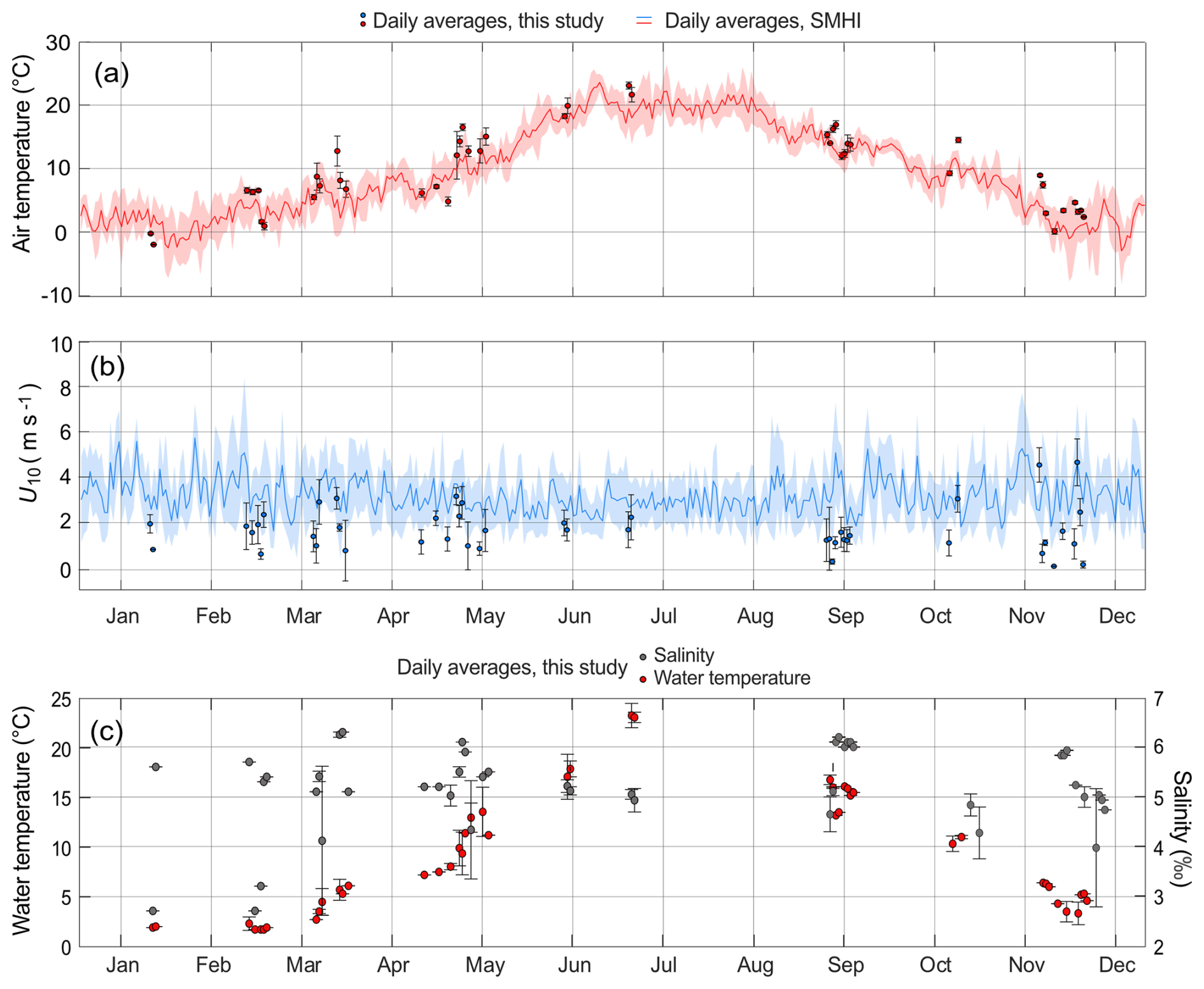
Figure 2 Daily average air temperatures (a), wind speeds at 10 m height, U₁₀ (b) and water temperatures and salinity (c). The local measurements during the flux sampling are shown as circle markers, with whiskers representing standard deviations. The plotted lines in (a) and (b) are daily average data from SMHI between the years 2020 and 2022. Shaded areas are standard deviations. x axis tick marks are on the 15 of every month.

Locally measured U₁₀ varied from near zero to 5.8 m s⁻¹, with an average of 1.6 ± 1.1 m s⁻¹ (Fig. 2b). Greater variability in local U₁₀ was observed from October to May, whereas measurements during June, July, and September were less variable. However, the monthly-averaged local U₁₀ did not exhibit a clear seasonal pattern. When compared to the SMHI wind data for the corresponding dates and times at Skarpö station, about 30 km to the northeast (Fig. 1), the local daily average U₁₀ was on average 44 % lower. Over the entire sampling campaign, the local average U₁₀ was 47 % lower than the SMHI station's long-term average between 2020 and 2022, which included both day- and nighttime data.

Observed surface water temperatures were between 1.7 and 24.5 °C (Fig. 2c), with the highest temperatures observed in July, and the lowest in January, similar to the air temperatures. Surface water salinity was between 2.3 ‰ and 6.3 ‰ (Table 1 and Fig. 2c), with > 90 % of observed salinities above 4.0. Salinities below 4.0 were measured between January and April, which was coinciding with the period following ice break-up and during spring snowmelt (Fig. 2c).

3.2 CO₂ sea-to-air fluxes

The sea-to-air CO₂ fluxes at each of the different sampling locations are shown in Fig. 3a. Omitting January where only two locations were sampled, the monthly average fluxes ranged from −937 ± 161 to 363 ± 87 mg CO₂ m⁻² d⁻¹ in the macroalgae-covered coarse sediment habitat (A), from −670 ± 8 to 1496 ± 68 mg CO₂ m⁻² d⁻¹ in the sparsely vegetated sand habitat (B), from −673 ± 27 to 1494 ± 77 mg CO₂ m⁻² d⁻¹ in the submerged plant-covered sand habitat (C), from −328 ± 17 to 1725 ± 139 mg CO₂ m⁻² d⁻¹ in the submerged plant-covered mixed substrate habitats (D and E), and from 294 ± 26 to 1757 ± 95 mg CO₂ m⁻² d⁻¹ in the reed-covered muds (F and G).

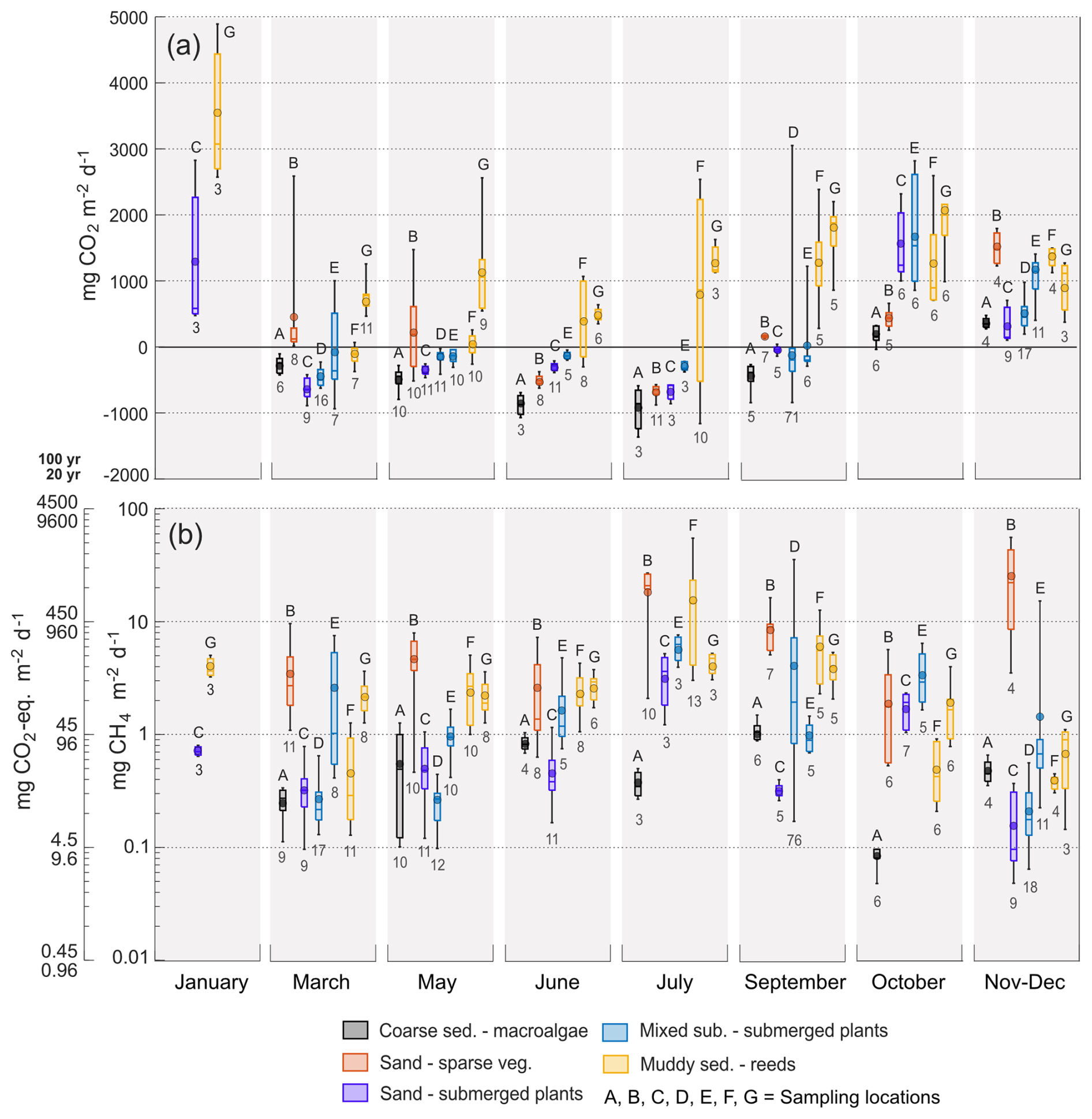
Figure 3 Boxplots with diffusive sea-air (a) CO₂ and (b) CH₄ fluxes from the chamber measurements, at each location and sampling period. CH₄ fluxes are plotted as both mg CH₄ m⁻² d⁻¹ and as mg CO₂-eq. m⁻² d⁻¹ over a 100 and 20 year time scale. Boxes represent 25th and 75th percentiles, lines within the boxes are the median, whiskers are 100th and 0th percentiles, circle markers are the mean. Note the logarithmic scale in (b). Numbers underneath the boxes are number of measurements and letters above are sampling location.

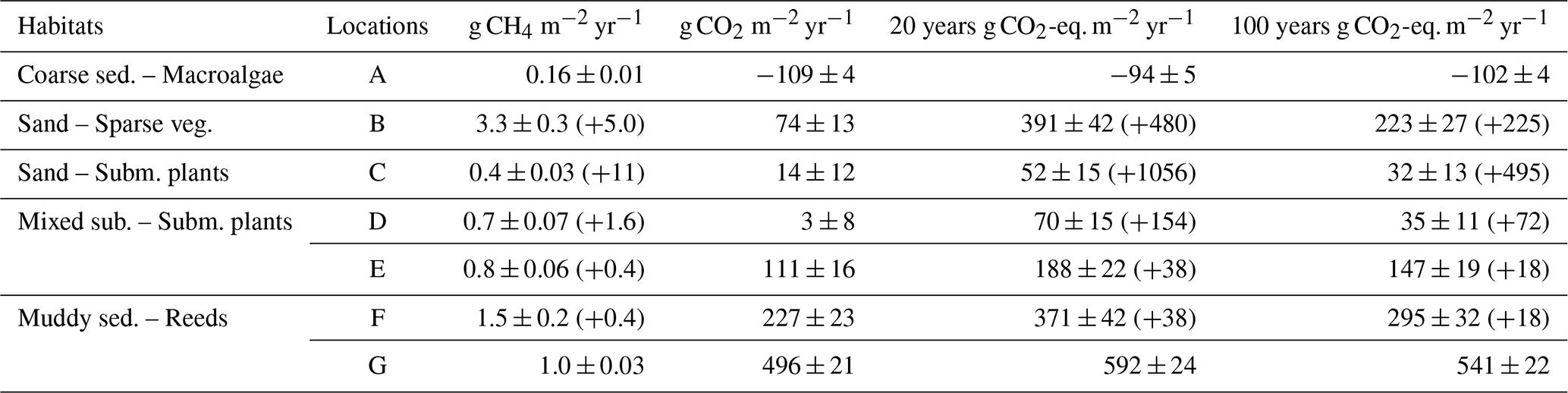
The macroalgae habitat (A), the submerged plant-covered sand habitat (C) and the mixed substrate habitats showed net CO₂ uptake throughout the warmer period of the year between March and September, while the sparsely vegetated sandy habitat (B) only took up CO₂ in June and July. The macroalgae habitat (A) was a net annual sink of −109 ± 4 g CO₂ m⁻² yr⁻¹ since it only emitted small quantities of CO₂ in the autumn months of October to December (Table 2, Fig. 3a). In the sand and mixed substrate habitats, the summer uptake was counterbalanced by high emissions in the autumn and winter months, so that these locations were acting as weak sources annually, spanning between 3 ± 8 and 111 ± 16 g CO₂ m⁻² yr⁻¹ (Table 2). The reed-covered muds differed from the other habitats by persistently showing net emission of CO₂, except for location F in March. Annually, this habitat was a relatively strong source of CO₂ between 227 ± 23 and 496 ± 21 g CO₂ m⁻² yr⁻¹ (Table 2). While seasonal changes in CO₂ fluxes were apparent in most habitats, the sensitivity of the fluxes to environmental parameters such as water temperature and wind speed was generally low (see Table S1).

Table 2 Yearly fluxes (diffusive and ebullitive) of CH₄, CO₂ and CO₂-equivalent flux of both CO₂ and CH₄ calculated for all locations. Uncertainties are given as standard errors of the mean. CH₄ ebullitive fluxes are within brackets.

In January the CO₂ emission from the two sampled locations, the submerged plant-covered sand habitat C, and the reed habitat G, were noticeably higher than during adjacent sampling periods of March and November–December. These elevated CO₂ fluxes in January corresponded with a time when the other locations and much of the coastline were ice-covered, while these locations were ice-free. The monthly average emissions in January in C and G were up to three times higher than those in March and November–December.

3.3 Diffusive CH₄ sea-to-air fluxes

All sampling locations were sources of CH₄ throughout the entire annual cycle (Fig. 3b). The average monthly diffusive sea-to-air CH₄ fluxes varied greatly between habitats. The macroalgae habitat (A) had the lowest flux, ranging from 0.1 ± 0.01 to 1.1 ± 0.1 mg CH₄ m⁻² d⁻¹, with no clear seasonal pattern. In contrast, the submerged plant-covered sand habitat (C) exhibited slightly higher fluxes, ranging from 0.2 ± 0.01 to 3.3 ± 0.3 mg CH₄ m⁻² d⁻¹, and displayed a clear seasonal trend, with elevated

fluxes during warmer months. The mixed substrate habitats (D and E) had fluxes ranging from 0.7 ± 0.1 to 4.6 ± 0.7 mg CH₄ m⁻² d⁻¹, and similar to sand habitat C the fluxes were higher in summer. The reed habitats (F and G) also showed increased fluxes in summer, but with a wider range from 0.5 ± 0.1 to 15 ± 3.6 mg CH₄ m⁻² d⁻¹. The sparsely vegetated sand habitat (B) had the highest fluxes overall, with monthly averages ranging from 2.3 ± 0.3 to 26 ± 11 mg CH₄ m⁻² d⁻¹. Similar to the macroalgae habitat (A), this habitat demonstrated little seasonal dependence, with the highest fluxes recorded during November–December. Annually, the diffusive CH₄ fluxes ranged from 0.16 ± 0.01 g CH₄ m⁻² yr⁻¹ in the macroalgae habitat (A) to 3.3 ± 0.3 g CH₄ m⁻² yr⁻¹ in the sparsely vegetated sand habitat (B) (Table 2). Significant relationships between diffusive CH₄ flux and water temperature were more consistent than for the CO₂ flux but had generally low predictability (see Table S1).

As observed for CO₂, the diffusive CH₄ fluxes from the ice-free locations in January were unusually high. Fluxes from the sand habitat C (0.7 ± 0.02 mg CH₄ m⁻² d⁻¹) were an order of magnitude higher, while fluxes from the reed habitat G (4.0 ± 0.3 mg CH₄ m⁻² d⁻¹) were approximately three times greater than the respective fluxes measured at these locations during November–December.

3.4 CH₄ ebullition

CH₄ ebullition was detected during measurements in all habitats except the macroalgae habitat (A) (Fig. 4) and while some ebullition was measured from March to October, most events were observed between July and September (Fig. 4c). During the ebullition events, the amount of CH₄ released per bubble ranged from 0.05 to 2688 µg (Fig. 4a), with both the lowest and highest values recorded in the submerged plant-covered sand habitat (C). The sparsely vegetated sand habitat (B) released between 332 to 1455 µg per bubble, which was significantly higher than that observed in the mixed substrate habitats (D and E) (1.2–679 µg) and the reed habitat (F) (36–151 µg).

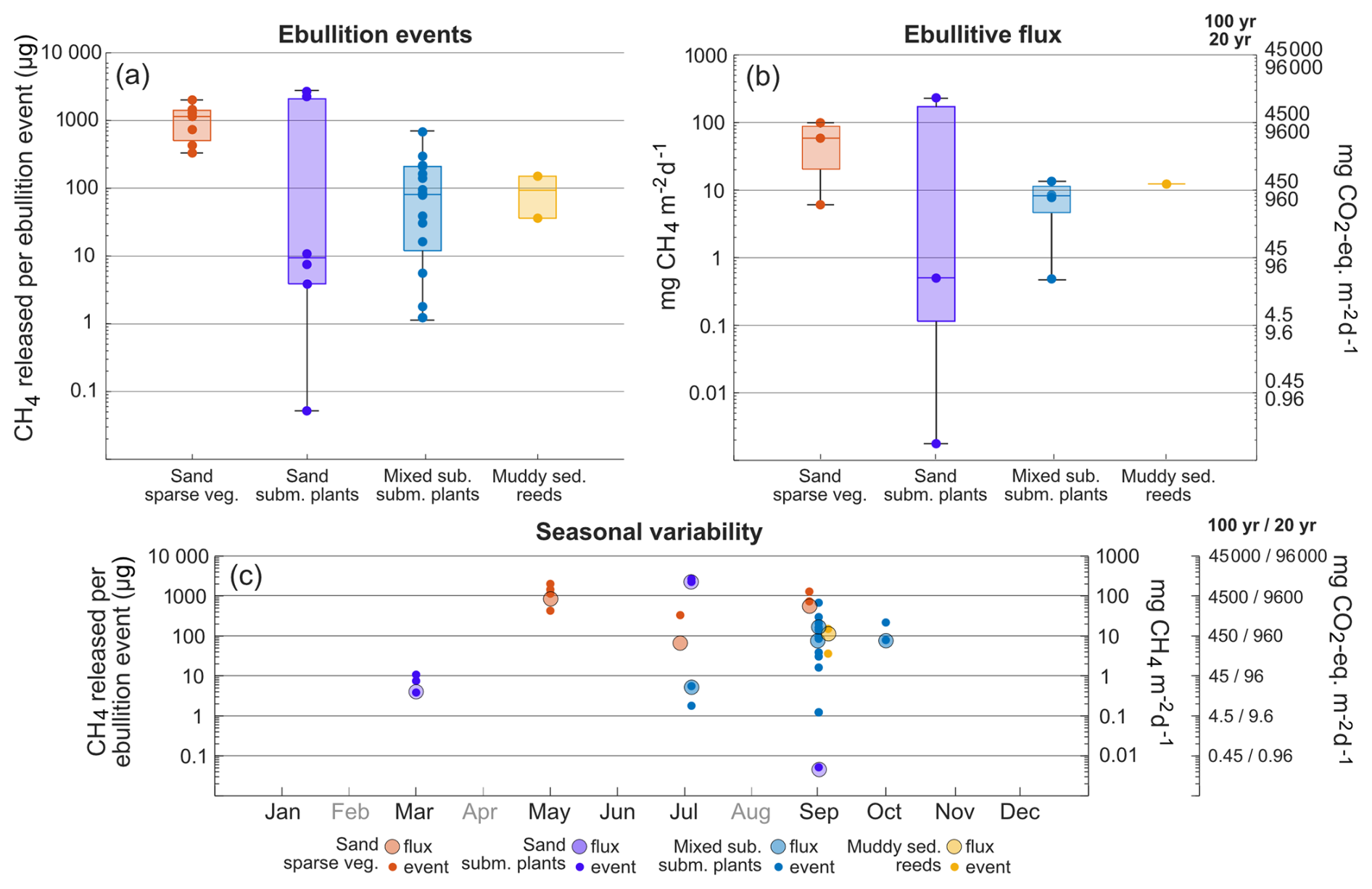
Figure 4 Boxplots with CH₄ released per ebulliton event (a) and CH₄ ebullitive flux calculated for a specific location and period, reported as CO₂-eq. flux as well (b). Boxes represents 25th and 75th percentiles, line within the box is the median, whiskers are 100th and 0th percentiles. Circle markers within boxplots are single events or single fluxes. CH₄ released per ebulliton event and CH₄ ebullitive flux is also plotted for the specific months where it was detected (c). Months that has not been sampled are in grey.

At the locations and during the months when ebullition was detected, between 4 %–40 % of the chamber experiments recorded ebullition. Extrapolating the ebullition over a 24 h period yielded CH₄ ebullitive fluxes between 0.001 and 232 mg CH₄ m⁻² d⁻¹ (Fig. 4b). The sparsely vegetated sand habitat (B) had ebullitive fluxes between 6 and 83 mg CH₄ m⁻² d⁻¹, the submerged plant-covered sand habitat (C) had the largest range from 0.001 to 232 mg CH₄ m⁻² d⁻¹, the mixed substrate habitats (D and E) ranged between 0.5 and 83 mg CH₄ m⁻² d⁻¹, and the reed habitat (G) had only one ebullitive flux recorded in September, 12 mg CH₄ m⁻² d⁻¹. No statistically significant differences could be found between the habitats, possibly due to the low number of calculated ebullitive fluxes, but generally the sand habitats showed the highest fluxes.

Ebullition was confined to depths of 3 m or less, with 90 % of events occurring at surface water temperatures above 11 °C. However, the magnitude of the ebullitive flux events did not consistently vary with either depth or temperature. Statistical analysis revealed inconsistency in the significance of the relationships between these variables and flux magnitude across the habitats (see Table S1). Thus, while depth and temperature thresholds may govern the onset of ebullition, they appear less influential on the magnitude of the flux within the ranges where ebullition was occurring. For the locations that showed bubble emission, between 0.3 % and 96 % of the total (ebullitive + diffusive) CH₄ flux could be attributed to ebullition for a specific sampling month. When extrapolating both fluxes over a year, assuming that ebullition was absent the months where the measurements did not detect it, the ebullitive flux accounted for between 21 % and 98 % of the total annual flux (Table 2).

3.5 Habitat differences and variability

The bootstrapping (Fig. 5) determined that the summer average CO₂ flux (May to September) in the macroalgae habitat (A) had a 95 % confidence interval of −720 to −481 mg CO₂ m⁻² d⁻¹, while the reed habitats (F and G) had an average between 575 and 1011 mg CO₂ m⁻² d⁻¹. These two habitats stood out as being statistically distinct at the 95 % level from any of the other habitats in summer (Fig. 5a). In contrast, the sparsely vegetated sand habitat (B), with a summer flux confidence interval of −386 to −48 mg CO₂ m⁻² d⁻¹ could not be differentiated from either the submerged plant-covered sand habitat (C) (−389 to −258 mg CO₂ m⁻² d⁻¹) or the mixed substrate habitats (D and E) (−202 to −36 mg CO₂ m⁻² d⁻¹). However, the latter two habitats did exhibit statistical differences from each other.

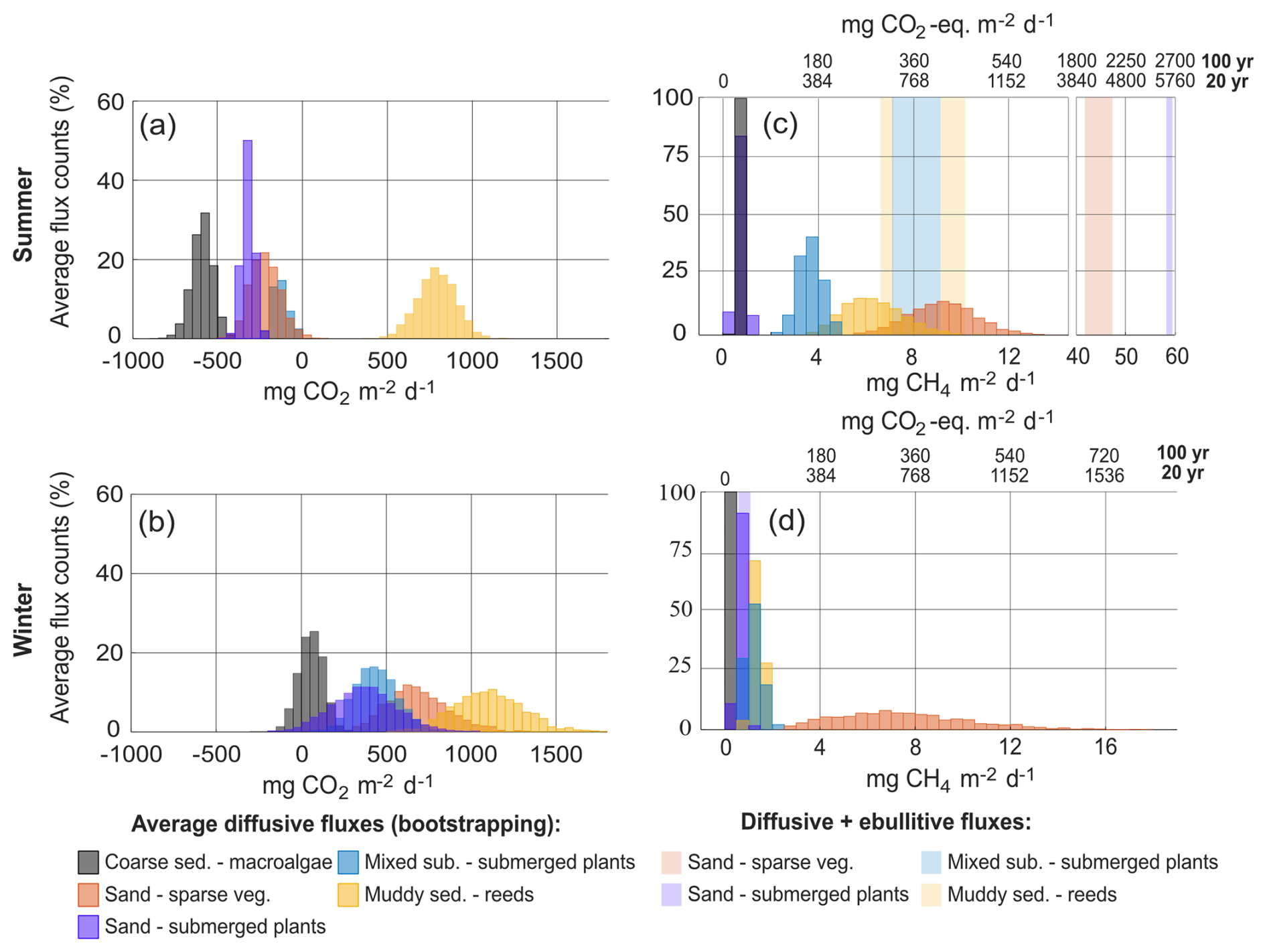
Figure 5 Average diffusive flux values obtained from the bootstrapping exercise for CO₂ (a, b) and CH₄ (c, d), divided up into the summer months May, June, July, and September (a, c) and winter months March, October, and November-December (b, d). January has been excluded since only two locations were sampled. The 95 % confidence intervals of the diffusive CH₄ have been added together with the average ebullitive flux and are displayed as pale blocks in (c) and (d).

During the ice-free months in winter (October, November, December, and March) none of the habitats had a distinct average CO₂ flux and each habitat overlapped at least one other habitat (Fig. 5b), although visual examination of the distributions of the average flux values indicates an increase from the macroalgae habitat (A) (−90 to 191 mg CO₂ m⁻² d⁻¹) followed by the submerged plant-covered sand habitat (C) (−91 to 631 mg CO₂ m⁻² d⁻¹), the mixed substrate habitats (D and E) (216 to 691 mg CO₂ m⁻² d⁻¹), the sparsely vegetated sand habitat (B) (375 to 1040 mg CO₂ m⁻² d⁻¹) and lastly the reed habitats (F and G) (677 to 1327 mg CO₂ m⁻² d⁻¹).

During summer, the average diffusive CH₄ flux in the macroalgae habitat (A) (0.5 to 0.9 mg CH₄ m⁻² d⁻¹) was indistinguishable from the submerged plant-covered sand habitat (C) (0.4 to 1.1 mg CH₄ m⁻² d⁻¹), although both these habitats were statistically distinct from the other habitats (Fig. 5c). However, when ebullition was included for the two sand habitats (B and C) the higher average total (diffusive + ebullitive) summer fluxes of around 45 and 60 mg CH₄ m⁻² d⁻¹, respectively, clearly separated these two habitats from the rest. The mixed substrate habitats (E and D) and the reed habitats (G and F) could not be distinguished from each other in summer when both ebullition and diffusion were considered, and both had an average flux centred around 8 mg CH₄ m⁻² d⁻¹. In winter, all habitats except the sparsely vegetated sand habitat (B) had an average flux under 2 mg CH₄ m⁻² d⁻¹, while the sand habitat (B) had a confidence interval between 3.1 and 14 mg CH₄ m⁻² d⁻¹ (Fig. 5d).

3.6 CO₂-equivalent fluxes

To calculate the CO₂-equivalent flux for CH₄ over a 20- and 100-year time period, the flux was multiplied by 96 or 45, respectively, to account for the sustained global warming potential of CH₄ (Neubauer and Megonigal, 2015). Considering both time scales, the CO₂-equivalent flux of CH₄ accounted for between 83 % and 99 % of the total radiative forcing added to the atmosphere from the sand habitats on an annual basis (B and C), between 33 % and 99 % from the mixed substrate habitats (D and E) and between 8 % and 45 % in the reed habitats (F and G) (Table 2). In the macroalgae habitat (A) the CO₂-equivalent flux of CH₄ offset the annual CO₂ uptake with between 7 % and 14 %. On a monthly basis, the CO₂-equivalent fluxes of CH₄ had the greatest impact in the summer months due to the contributions from ebullition (Fig. 6).

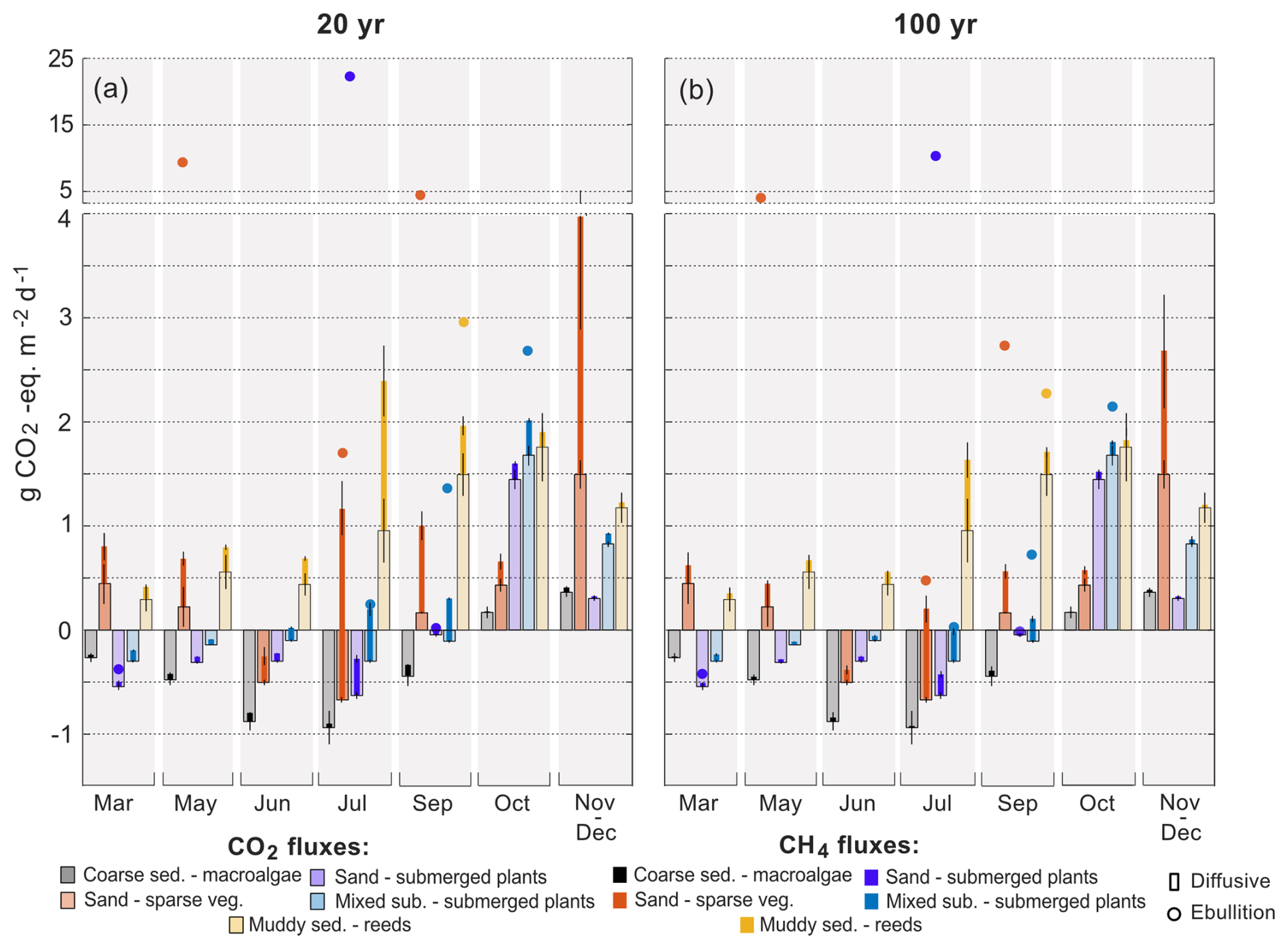
Figure 6 Diffusive CO₂ and CH₄ as average habitat CO₂-equivalent fluxes for each sampling period, except January when only two locations were sampled, for both a 20-year time period (a) and 100-year time period (b). The CO₂-equivalent CH₄ ebullitive fluxes are not averages for each habitat but plotted as the calculated values for each location containing ebullition. Note the broken y axis. CH₄ fluxes (diffusive + ebullitive) are stacked on the CO₂ fluxes and therefore represent the flux value of both gases. Error bars are the standard error of the mean.

4 Discussion

4.1 Sediment and vegetation type as predictor for flux

It is well known that the shallow-water coastal zone has significant variability in CO₂ and CH₄ fluxes that can span two orders of magnitude over short spatial (< 50 m) and temporal (< 24 h) scales (Asmala and Scheinin, 2023; Roth et al., 2023). This variability complicates efforts for quantification and upscaling of the coastal contribution to the atmospheric budget. To address this, we assessed whether these fluxes could be reliably constrained by habitat types of the Baltic Sea defined within HELCOM HUB (HELCOM, 2013). Linking flux variability to habitat types offers a potential pathway to streamline upscaling efforts.

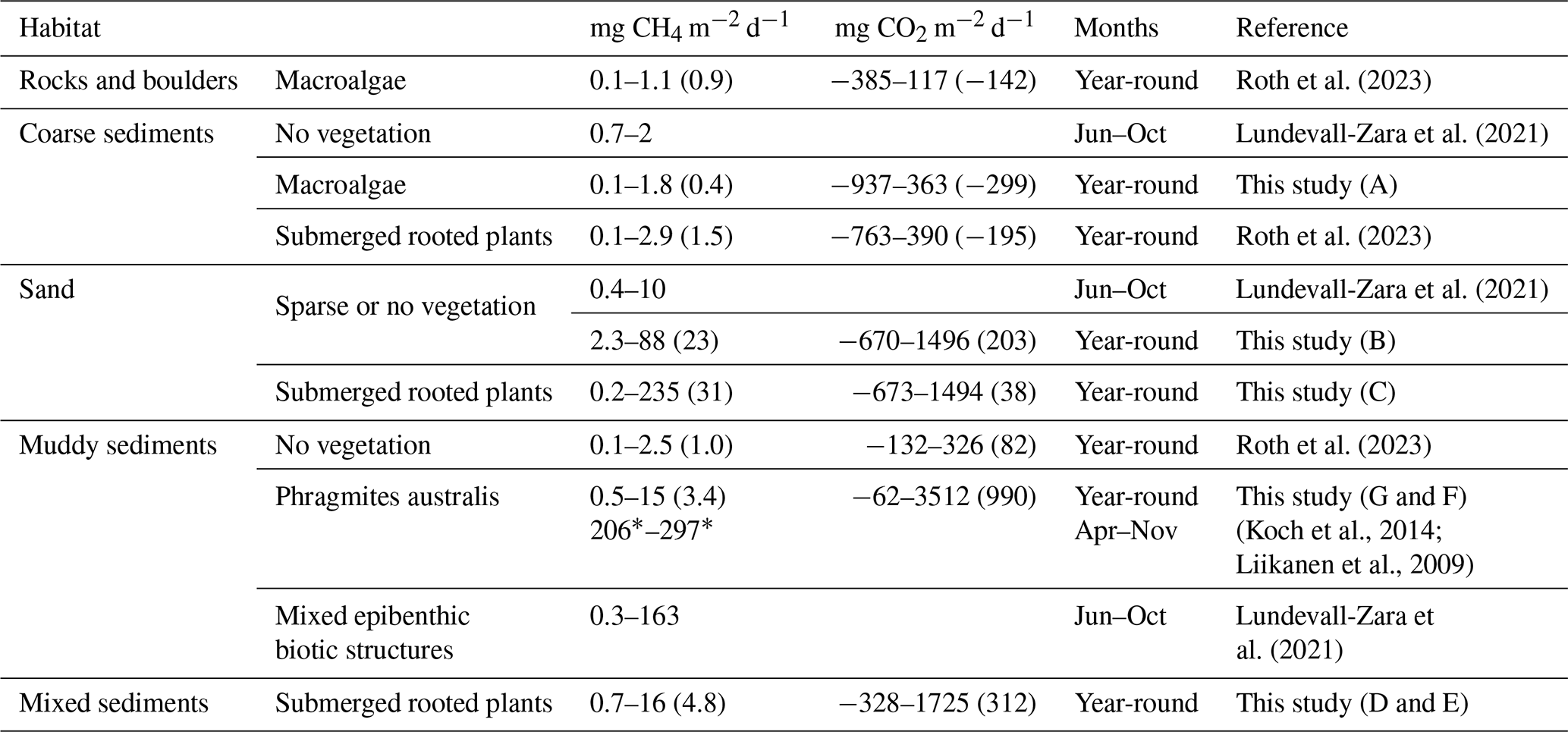
Coarse sediment habitats with macroalgae demonstrated low CO₂ and CH₄ flux variability and a total absence of CH₄ ebullition, likely reflecting limited organic matter deposition and restricted rates of sediment respiration and methanogenesis (Chen et al., 2022). Our measurements within this habitat exhibited annual net CO₂ uptake that agrees with prior studies of similar environments, including macroalgae on rocks and boulders and submerged rooted plants on coarse sediment (Roth et al., 2023). The CH₄ fluxes also align well with other studies of coarse sediments in the Baltic Sea differing by less than 1.1 mg CH₄ m⁻² d⁻¹ (Lundevall-Zara et al., 2021; Roth et al., 2023) (Table 3). This consistency positions coarse sediment as a robust reference category for regional CO₂ and CH₄ flux scaling. Moreover, their similarity to rock and boulder habitats suggests potential for broader classification schemes.

Table 3 Sea-to-air CO₂ and/or CH₄ (diffusive + ebullitive) fluxes in shallow, near-shore waters (mean depth < 4 m) in the Baltic Sea, where the study periods have stretched at least a few months. Fluxes are reported as the range of monthly averages and with annual averages within brackets where available, if not denoted with a *, in which case it is an average over the whole study period.

Reed-dominated muddy habitats displayed greater variability in CO₂ fluxes. While brackish wetlands with Phragmites vegetation are typically reported as CO₂ sinks in summer outside the Baltic Sea (Martin and Moseman-Valtierra, 2015; Sanders-DeMott et al., 2022), this study found predominantly net emissions during summer. Persistent CO₂ oversaturation during all seasons distinguishes the habitat in this study and likely reflects high remineralisation rates of either allochthonous or autochthonous carbon (Chen et al., 2022). While CO₂ fluxes of this habitat type are less consistent with the existing literature, the clear deviation from the other habitats in this study underscores the need for a separate categorisation.

The sand and mixed substrate habitats, despite their variable submerged plant composition, exhibited overlapping CO₂ flux ranges and similar seasonal dynamics, indicating broadly comparable biogeochemical characteristics. While differences in primary production, respiration, and carbon burial, linked to the vegetation community may exist and could be responsible for a part of the variability in flux magnitudes or temporal patterns (Gattuso et al., 1998), these differences appear insufficient to separate the habitats in terms of the averaged flux. Consequently, for large-scale flux estimations or upscaling efforts, detailed knowledge of vegetation community composition or sediment grain size may be less critical for predicting the CO₂ flux. Instead, focusing on dominant habitat features, such as overall sediment type and general vegetation presence, could provide a sufficiently practical and reliable framework for flux prediction in these habitat groups.

CH₄ winter fluxes were consistently low across all habitats, aligning with the temperature sensitivity of methanogenesis (Yvon-Durocher et al., 2014). Habitat differences appeared less influential during this season, although the sparsely vegetated sand habitat exhibited anomalously elevated and variable fluxes with a 10 mg CH₄ m⁻² d⁻¹ confidence interval of the average winter flux. This outlier may reflect unaccounted drivers or localised factors not described by the HELCOM classification.

In summer, CH₄ flux variability increased drastically, mainly due to ebullition which amplified total fluxes by up to an order of magnitude. Our findings suggest that, in the coastal shallow-water zone, the variability in diffusive CH₄ fluxes may be of secondary importance when compared to the significant contribution of sea-air ebullition. Bubble emission not only overshadowed diffusive flux variability but also defined the upper limit of the flux magnitude in many habitats, similar to previous findings in the Baltic Sea shallow-water zone (Lundevall-Zara et al., 2021). The upper limits of CH₄ fluxes in sand, mixed substrate and muddy sediment habitats are variable between the studies performed in the Baltic Sea (Table 3), but are up to two orders of magnitude higher for the studies using floating chambers which can incorporate the bubble flux (Liikanen et al., 2009; Koch et al., 2014; Lundevall-Zara et al., 2021) than for the studies using concentration gradients between the water and air and then calculate a diffusive flux (Roth et al., 2023).

Contradicting previous findings that the majority of ebullition comes from muddy, organic-rich sediments (Crawford et al., 2014; Lundevall-Zara et al., 2021), this study identified the sand habitats as those most prone to ebullition. While it cannot be rules out that organic-rich sediment underlies the sand and contributes to the ebullition, the finding shows that assumptions that widespread ebullition is isolated to a habitat that would be classified as a muddy sediment habitat will underestimate the area of the coastline that exhibits intense CH₄ ebullition.

4.2 Constraining the ebullitive flux

The ebullition data from this study not only corroborate previous findings that CH₄ ebullition dominates coastal CH₄ emissions (Weber et al., 2019), but further demonstrates that ebullition could be the dominant component of the coastal shallow-water carbon-based greenhouse gas flux. Most of the previous estimates for coastal CO₂ and CH₄ fluxes in the Baltic Sea have relied on bulk methods based on sea-air concentration gradients and k parameterisation (e.g. Ma et al., 2020; Roth et al., 2022; Asmala and Scheinin, 2023). While effective for assessing diffusive exchange, and hence also for the sediment-derived gas ebullition that subsequently dissolves in the water column (Hermans et al., 2024), these approaches fail to account for direct bubble-mediated transport across the water-air interface, thereby leading to systematic underestimation of coastal CH₄ fluxes.

A common characteristic of ebullition studies in near-shore waters, including this one, is the large range of the observed fluxes which typically vary by over four orders of magnitude (Lundevall-Zara et al., 2021; Wang et al., 2021; Żygadłowska et al., 2024). However, our findings indicate that habitat type provides a useful predictor of both the frequency of ebullition events and, to a lesser extent, the amount of CH₄ released per event. This suggests that habitat-based classifications could serve as a valuable tool for constraining ebullitive flux estimates, offering a more structured framework for quantifying CH₄ emissions in coastal ecosystems.

A key challenge remains in scaling episodic ebullition events into time- and space-averaged fluxes. Variability in bubble size, release frequency, and lateral distribution introduces significant uncertainty in determining representative flux values. Consequently, the methodological approach used to integrate ebullition events into broader estimates can significantly influence reported fluxes. Nevertheless, our results align with previous observations from a eutrophic coastal basin of the North Sea (Żygadłowska et al., 2024), and from the island of Askö in the Baltic Sea (Lundevall-Zara et al., 2021). Reported ebullitive fluxes in the North Sea study were up to 3920 mg CH₄ m⁻² d⁻¹, while at Askö the average monthly ebullitive and diffusive fluxes were up to 163 mg CH₄ m⁻² d⁻¹. The maximum monthly diffusive and ebullitive flux observed in this study (235 mg CH₄ m⁻² d⁻¹) falls within the same range, despite differences in methods used to integrate ebullition into time-averaged estimates.

4.3 The importance of winter fluxes for the annual budget

In January, the emission fluxes of both CO₂ and CH₄ at ice-free locations were high despite the coldest water temperatures of the sampling campaign, when both methanogenesis and respiration are expected to be lowest (Thamdrup et al., 1998; Yvon-Durocher et al., 2014). While wintertime efflux of CO₂ is expected to be higher compared to summertime when photosynthesis counteract the respiration, peak CO₂ emissions are usually observed in the autumn when temperatures are still sufficient for elevated respiration, but photosynthesis has decreased (Honkanen et al., 2024; Lainela et al., 2024). However, the CO₂ fluxes in January were substantially higher than in October in this study. Furthermore, since the solubility of CO₂ and CH₄ increases with decreasing water temperature, it should result in less outgassing to the atmosphere (Lucile et al., 2012; Guo and Rodger, 2013).

Previous studies have found increased gas fluxes following ice breakup in aquatic environments and suggested it to be a period of significant contribution to the annual flux budget (Jansen et al., 2019; Wang et al., 2023). During ice-covered periods, dissolved gas and bubbles accumulate under the ice, with little-to-no sea-air exchange and limited oxidation of CH₄ due to the low temperatures. The accumulated gas is later allowed to escape during ice-breakup (Denfeld et al., 2018; Roth et al., 2022). In our study, no active ice-melt or break-up was observed at the time of sampling, and ice observations were not made prior to the sampling periods. We speculate that the higher fluxes may be due to earlier ice-breakup, or horizontal transport of water from ice-covered areas.

Assuming that this elevated flux would persist for half a month to a full month (depending on whether it originates from previous local ice breakup or from transport from other ice-covered areas), its contribution to the annual exchange of CO₂ would range between 10 % and 22 %, and between 3 and 12 % to the annual diffusive emission of CH₄. However, from the perspective of the coastal greenhouse gas budget, these emissions may simply represent a shift in the timing or location of release rather than an overall increase in total flux. Establishing baseline winter emissions of CO₂ and CH₄ during ice-free conditions may suffice for budgetary assessments, as the presence of ice would primarily redistribute these emissions across time and space rather than add to the annual total emission.

4.4 Coastal CO₂ and CH₄ budget of the Stockholm archipelago

Given the diversity of habitats along the Baltic Sea coastline and the relatively high anthropogenic pressure on the Stockholm archipelago (Hill and Wallström, 2008; Kautsky, 2008), extrapolation beyond this region could introduce large uncertainties. The Stockholm archipelago, which absorbs much of the city's anthropogenic load, differs from other urban coastal areas in the Baltic Sea, where habitat-specific flux ranges must be assessed independently. However, despite this regional specificity, the archipelago holds roughly one-fourth of Sweden's total coastline (mainland and islands) (Statistics Sweden, 2020), making it representative of a significant portion of the Swedish near-shore shallow-water zone.

The agreement of the temperature and wind data between the SMHI record (SMHI, 2024a, b) and the local measurements suggests that the dataset has captured the seasonal cycle in the area, with deviations likely arising from differences in geographical settings of the SMHI stations and the sampling locations, as well as shorter averaging periods of the local measurements. However, we note that sampling was limited to wind speeds below 5.8 m s⁻¹. Due to the commonly suggested non-linear dependence of gas transfer on wind speed (Wanninkhof et al., 2009), infrequent high wind periods may disproportionately influence the average flux.

Another source of uncertainty is the absence of nighttime flux data. While diurnal variations in CH₄ fluxes have been observed in coastal waters of the Baltic Sea (Roth et al., 2022) and on Sweden's west coast (Henriksson et al., 2024), daytime increases were inconsistent across habitats and months. Further, reported CH₄ variability generally falls within the diffusive bootstrapping confidence interval for summertime fluxes in this study (0.02 to 6 mg CH₄ m⁻² d⁻¹), making it a minor uncertainty compared to the ebullitive flux. For CO₂ fluxes, photosynthesis is expected to peak in the summer afternoons which may have led to a slight overestimation of uptake (Roth et al., 2023), although measured summer CO₂ fluxes in this study align with prior estimates for coastal habitats which include nighttime values (Honkanen et al., 2024).

Despite these uncertainties, the dataset can provide a first estimate of the coastal shallow-water sea-air gas budget for the Stockholm area. Mattisson (2005) mapped the Stockholm archipelago based on the EUNIS classification scheme (Davies et al., 2004), a habitat classification scheme developed for Europe, and compatible with the HELCOM HUB, with the difference that the latter was specifically developed for the Baltic Sea (HELCOM, 2013). The mapping found that the most common habitat groups in shallow waters (< 6 m) were bedrock or coarse sediments, which take up 40 % of the area (total mapped area: 681 km²). Applying the annual flux of the coarse sediment with macroalgae habitat to this area yields fluxes of −30 Gg CO₂ yr⁻¹ and 0.04 Gg CH₄ yr⁻¹. Reed beds account for 1.6 % of the total area, and muddy sediments without specified vegetation account for another 18 %. Applying the fluxes from the muddy sediment with reeds habitats yields fluxes of between 30 and 67 Gg CO₂ yr⁻¹ and 0.01 to 0.03 Gg CH₄ yr⁻¹. Sublittoral sand, with or without vegetation (not distinguished in Mattisson, 2005), covers 2 % of the shallow water area. Applying the lowest and highest flux estimate for the sand habitat yields fluxes ranging between 0.04 and 1.7 Gg CO₂ yr⁻¹ and 0.1 and 0.2 Gg CH₄ yr⁻¹. The remaining 38 % is described as a mixture of consolidated clay, bedrock, and more mobile sediments, but is not described in terms of its vegetation. Applying the highest and lowest values from the annual fluxes from the coarse sediment habitat, the sand habitats and the mixed substrate habitats yields a large possible range of −28 to 29 Gg CO₂ yr⁻¹ and 0.04 to 2.9 Gg CH₄ yr⁻¹.

Combining both CO₂ and CH₄ fluxes, the CO₂-equivalent flux of the shallow-water coastal zone in the Stockholm archipelago adds up to between 0.005 and 0.4 Tg CO₂-eq yr⁻¹ and between −0.01 and 0.2 Tg CO₂-eq yr⁻¹ over a 20- or 100-year time period, respectively. At a regional scale, the Stockholm urban area emits approximately 1.2 Tg CO₂-eq yr⁻¹ (100-year timescale) from the energy and transport sectors alone (Stockholms stad, 2024). While the coastal zone's emissions are small by comparison, its contribution to the regional carbon budget still has the potential to offset efforts to reduce overall emissions.

4.5 Implications for the coastal zone as a tool in climate mitigation

Distinguishing between air-sea fluxes and sediment carbon sequestration is crucial for accurately determining and communicating the climate mitigation potential of a habitat (Johannessen and Christian, 2023). While most of the sampling locations show a net efflux of CO₂ to the atmosphere, they could still sequester organic carbon. An aquatic system can act as both a sink for organic carbon in the sediments and at the same time show net sea-air CO₂ and CH₄ emissions to the atmosphere, due to the addition of allochthonous carbon that subsidises habitat respiration, indicating that these two properties are not always linked (Santoso et al., 2017). In fact, the coarse sediment with macroalgae habitat that showed the highest net uptake of CO₂ most likely has the lowest sediment carbon sequestration due to the exposed setting, limiting deposition. While it is true that carbon buried in anoxic sediments can be stored and isolated from atmospheric exchange for 1000+ years (Dahl et al., 2024), it is the actual exchange at the sea-air interface that directly affects atmospheric concentrations (Van Dam et al., 2021).

Integrating the carbon burial in coastal sediments into Nationally Determined Contributions (Herr and Landis, 2016) or in carbon trading (Claes et al., 2022) as a means of offsetting fossil fuel CO₂ emissions, without simultaneously accounting for the coastal sea-air exchange, risks undermining national and global climate targets (Williamson and Gattuso, 2022). Including the coastal zone in national carbon budgets is therefore more complex than the terrestrial environment and should in all cases include simultaneous measurements of CO₂ and CH₄ over the sea-air boundary layer. As evident from the results in this study, CH₄ can play a substantial, if not dominant, role in the annual exchange and should be assessed with a method that can account for the ebullition component of the flux as well.

5 Conclusions

The study quantified seasonal and annual fluxes of CO₂ and CH₄ from five distinct coastal, shallow water habitat types (macroalgae-covered coarse sediments, sparsely or densely vegetated sands, submerged plant-covered mixed substrates, and reed-dominated muds) in the archipelago surrounding Stockholm and Trosa along the central Baltic Sea coast. Significant differences between the flux distributions in the various habitats were found for both diffusive CO₂ and CH₄ fluxes, primarily in summertime. Macroalgae-covered coarse sediments and reed-dominated muds stood out as having distinct CO₂ flux ranges, whereas the other three habitats showed more similarities. The occurrence of CH₄ ebullition and variation in flux magnitude allowed for a clear distinction between the habitats where the sand habitats had the highest emissions, followed by the reeds and mixed substrate habitats and lastly, the macroalgae habitat. The annual net CO₂-equivalent exchange indicated that four out of five habitats were net sources of CO₂ and CH₄ to the atmosphere where CH₄ ebullition dominated the exchange in three out of five habitats. An initial estimate of the budget of carbon-based greenhouse gases in the shallow-water coastal zone of the Stockholm archipelago suggests that this area is likely a weak source of carbon-based greenhouse gases to the atmosphere, with a range of 0.005 to 0.4, or −0.01 to 0.2 Tg CO₂-eq yr⁻¹ over a 20- and 100-year time scale respectively.