Environmental drivers constraining the seasonal variability in satellite-observed and modelled methane at northern high latitudes

Methane emissions from Northern Hemisphere high-latitude wetlands are associated with large uncertainties, especially in the rapidly warming climate. Satellite observations of column-averaged methane concentrations (XCH₄) in the atmosphere exhibit variability due to time-varying sources and sinks as well as atmospheric transport. In this study, we investigate how environmental variables, such as temperature, soil moisture, snow cover, and the hydroxyl radical (OH) sink of methane, explain the seasonal variability in XCH₄ observed from space over Northern Hemisphere high-latitude wetland areas. We use XCH₄ data obtained from the TROPOMI instrument aboard the Sentinel-5 Precursor satellite, retrieved using the Weighting Function Modified Differential Optical Absorption Spectroscopy (WFMD) algorithm. In addition, we perform the analysis using two atmospheric inversion model configurations: one based on non-optimized prior fluxes and another using fluxes optimized with in situ atmospheric observations. The aim was to assess the consistency between satellite-based and model-based results and to explore differences in how environmental variables drive the variability in XCH₄.

Environmental variables are derived primarily from meteorological reanalysis datasets, with satellite-based data used for snow cover and soil freeze–thaw dynamics and modelled data used for the OH sink. Our analysis focuses on five wetland-dominated case study regions over Northern Hemisphere high latitudes, including two in Finland and three in Russian Siberia, covering the period from 2018 to 2023.

Our findings reveal that environmental variables have a systematic impact on satellite-based XCH₄ variability. Seasonal variability is primarily driven by the OH sink and snow, particularly the snow water equivalent, while daily variability is most strongly affected by air temperature. The results are largely consistent with local in situ studies, although the role of snow appears more pronounced in our analysis. We observe interesting differences in the environmental drivers influencing satellite-based and model-based XCH₄. The posterior results after in situ data assimilation were better aligned with the satellite-based results than the prior, suggesting that, while there remains room for improvement in model priors and configurations, there is already some consistency between the modelled and observed total-column methane dynamics. However, the prior fluxes used in the model could benefit from improved snow information.

Overall, our results demonstrate how satellite-based XCH₄ observations can be used to study the seasonal variability in atmospheric methane over large wetland regions. The results imply that satellite observations of atmospheric composition and other Earth observations and meteorological reanalysis data can be jointly informative with respect to the processes controlling emissions in Northern Hemisphere high latitudes.

1 Introduction

Methane (CH₄) is the second most important anthropogenic greenhouse gas (GHG), in terms of its total radiative forcing, following carbon dioxide (CO₂). In recent decades, methane concentrations in the atmosphere have experienced a rapid growth rate, the drivers of which are being debated (e.g. Turner et al., 2017; Skeie et al., 2023). The highest growth rates were observed in 2020–2021; this has been explained by increased emissions from wetlands in both the tropics and high Northern Hemisphere latitudes (Peng et al., 2022; Zhang et al., 2023; Feng et al., 2023; Qu et al., 2024). Globally, approximately 65 % of methane emissions are anthropogenic, with agriculture and waste management being the primary contributors (Saunois et al., 2025; Jackson et al., 2024). The main natural source is wetlands and inland freshwater systems. The main sink of methane is chemical loss by hydroxyl radicals (OH), primarily in the troposphere. According to Saunois et al. (2020, 2025), 65 % of the global emissions originate from south of 30° N, and methane emissions from high latitudes (north of 60° N) represent only 4 % of the global total. However, uncertainties in the high-latitude regions are notably larger, with atmospheric-measurement-based top-down estimates having uncertainties exceeding ± 20 %, compared to less than ± 5 % globally. Since 1979, the high Northern Hemisphere latitudes have been warming nearly 4 times faster than the global average (Rantanen et al., 2022), a phenomenon with potentially significant consequences for methane emissions in these sensitive areas: for example, a warming climate can lead to an extended growing season or longer shoulder seasons, during which emissions are higher on a monthly basis, compared to colder months (Zona et al., 2015; Bao et al., 2021; Rößger et al., 2022). Additionally, warming can directly increase methane emissions from specific land cover types (Rehder et al., 2023) or thaw permafrost, potentially leading to rising emissions, as regions with less permafrost have been found to have lower methane fluxes compared to continuous-permafrost regions (Erkkilä et al., 2023; Rößger et al., 2022).

Seasonal variability in the methane concentration in the Northern Hemisphere is driven by the seasonality of its sinks and sources, whereas the sink dominates in the Southern Hemisphere (East et al., 2024). Although anthropogenic methane emissions show seasonal variability in the high latitudes in some sectors (Tsuruta et al., 2023), likely related to factors such as gas production or biomass burning (Berchet et al., 2015), natural emissions show much stronger seasonal variability, mainly driven by wetland emissions (East et al., 2024; Tsuruta et al., 2023). Methane emissions from wetlands are influenced by wetland conditions and environmental variables, including, for example, temperature (Howard et al., 2020; Rinne et al., 2018; Kittler et al., 2017), soil moisture and water table level (Virkkala et al., 2024), and snow cover and soil frost (Rößger et al., 2022; Zona et al., 2015; Mastepanov et al., 2013; Rinne et al., 2007). The methane emissions from wetlands are primarily driven by anaerobic processes, where methanogens produce methane by reducing carbon dioxide with hydrogen or breaking down acetate (Bridgham et al., 2013). Such processes are sensitive to environmental conditions that can limit microbial activity, particularly through changes in water availability. Both overly dry and overly wet soils can reduce microbial activity, as suitable moisture levels are required for microbial decomposition. Freezing of the soil, in particular, can limit the availability of liquid water, slowing microbial processes. Furthermore, the main sink of methane, oxidation by OH radicals, has a strong seasonality driven by the number of OH radicals, which is influenced by seasonal variations in their production: OH is primarily produced by the photolysis of ozone in the presence of water vapour, and its concentration fluctuates with factors such as temperature, humidity, and UV radiation (Zhao et al., 2019; Travis et al., 2020). These meteorological factors vary seasonally, especially in the middle and high latitudes, leading to seasonal variation in the OH sink. Additionally, when considering methane concentrations throughout the atmosphere, transport must be accounted for due to methane's lifetime of approximately 9 years (Saunois et al., 2025). Transport patterns can affect the seasonal variability in methane over long timescales, and changes in transport patterns and emissions in other regions might influence observed concentrations elsewhere (Dowd et al., 2023).

The seasonal variability in methane has often been studied using in situ measurements and models. In situ measurements can accurately measure the methane concentration or flux at a single point close to the ground or in a tower. The advantage of these measurements lies in their high accuracy and continuous time series, allowing the use of a network of stations for precise calculations of the regional or global methane budget. However, gaps in the measurement network hamper the precise localization of emissions, and the results are difficult to extrapolate to larger areas. This is because in situ flux measurements often represent specific conditions, such as particular land cover, vegetation type, soil humidity, and local climate. Additionally, these measurements require electricity and access to the measurement site; therefore, the flux measurements are often limited to the thaw and snow-free seasons for maintenance reasons. Models, in contrast, can describe large-scale phenomena, but they require comprehensive observations to model processes accurately.

The use of satellites in GHG studies has been possible since the 2000s. Satellite observations of methane concentrations in the near-infrared wavelengths started in 2002, when SCIAMACHY was launched aboard Envisat (Buchwitz et al., 2005). The Greenhouse Gases Observing Satellite (GOSAT), launched in 2009, was the first satellite dedicated to GHG observations (Kuze et al., 2009), followed by the TROPOspheric Monitoring Instrument (TROPOMI) aboard the Copernicus Sentinel-5 Precursor satellite in 2017. In addition to these missions, small satellites such as GHGSat also measure methane concentrations, but their utility for large-scale analysis is limited due to their narrow swath and infrequent revisit times. From SCIAMACHY to TROPOMI, both the spatial and temporal resolutions have significantly improved; for example, pixel sizes have decreased from tens of kilometres to a few kilometres, and revisit times have been reduced from several days to 1 d.

Satellites observe the column-averaged dry-air mole fraction of methane (XCH₄), which is retrieved from solar radiation in the near-infrared wavelengths reflected by the atmosphere or ground surface. Therefore, satellite observations of methane are dependent on sunlight. At high latitudes, the lack of sunlight causes a so-called winter gap in GHG satellite observations, as measurements cannot be conducted due to the Sun being close to or beyond the horizon. In addition to large solar zenith angles, cloud cover presents challenges for retrieval algorithms. Additionally, surfaces with a spectrally dependent reflectance, such as snow cover (Mikkonen et al., 2024), can introduce retrieval errors (Lorente et al., 2022). Despite these factors that limit data availability in the Northern Hemisphere high latitudes, updated and improved retrieval algorithms and the high spatial coverage of TROPOMI have reduced the length of the winter data gap in these regions. For the latest version of Weighting Function Modified Differential Optical Absorption Spectroscopy retrievals (WFMD v1.8; Schneising et al., 2019, 2023), the observational coverage is, in principle, gapless when considering areas above 50° N overall (Lindqvist et al., 2024). Satellite observations of methane have been used in a wide range of studies, for example, to identify the location and intensity of local point sources (Vanselow et al., 2024; Barré et al., 2021) as well as to investigate variations in methane trends (Hachmeister et al., 2024; Kivimäki et al., 2019). Additionally, methane satellite retrievals have been widely utilized to inform inversion models on methane concentrations (e.g. Tsuruta et al., 2023; Liang et al., 2023; Pandey et al., 2016).

In this study, we investigate how environmental variables explain the seasonal variability in satellite-observed column-averaged methane concentrations over high-latitude wetland areas. As shown by East et al. (2024), the seasonal methane cycle in the Northern Hemisphere remains poorly understood due to gaps in wetland emission inventories. Satellite observations of methane concentrations can offer a more detailed view, both spatially and temporally, of the processes shaping this cycle in high northern wetlands. Our aim is to determine how (1) environmental variables related to methane emissions and (2) methane loss by OH influence total-column concentrations. Based on the in situ measurement findings presented above, we focus particularly on the roles of temperature, soil moisture, snow cover, soil freeze and thaw, and the impact of the OH sink, while also examining whether our results align with these in situ findings. In addition, we assess the consistency of satellite-based results and those from an atmospheric inverse model optimized with in situ measurements of methane. The purpose is to compare the variability in column-averaged methane concentrations as driven by the environmental variables. The model simulations are performed using the CarbonTracker Europe – CH₄ (CTE-CH₄; Tsuruta et al., 2017) system and include two configurations: (1) a forward simulation using prior (non-optimized) fluxes and (2) an inversion simulation in which fluxes have been optimized using in situ atmospheric observations. In Sect. 2, we introduce the datasets used; the methods are given in Sect. 3; Sect. 4 presents and discusses the results; and the conclusions are presented in Sect. 6.

2 Datasets

2.1 TROPOMI WFMD XCH₄ product

The TROPOspheric Monitoring Instrument (TROPOMI) aboard the Copernicus Sentinel-5 Precursor (S5P) satellite was launched in October 2017 and is dedicated to producing observations for air quality and climate monitoring. With its wide swath of approximately 2600 km, a daily global coverage can be attained. Currently, two retrieval algorithms are generated to retrieve the column-averaged dry-air mole fraction of methane (XCH₄) from the near-infrared spectra: the operational TROPOMI XCH₄ product, developed by the SRON Netherlands Institute for Space Research (Hu et al., 2018; Lorente et al., 2021), and the Weighting Function Modified Differential Optical Absorption Spectroscopy (WFMD) algorithm, developed by the University of Bremen (Schneising et al., 2019, 2023). In this study, we use XCH₄ concentrations retrieved by the WFMD algorithm due to its accuracy and suitability for our analysis (University of Bremen, Institute of Environmental Physics, 2024). The WFMD v1.8 product shows no seasonal bias when comparing it to high-latitude ground-based observations and AirCore data, resulting in a lower mean bias and standard deviation (Lindqvist et al., 2024). Furthermore, the WFMD product provides significantly more data from high Northern Hemisphere latitudes, particularly during the spring months, and features a shorter winter gap.

The WFMD algorithm simultaneously retrieves the column-averaged dry-air mole fractions of CH₄ and carbon monoxide (CO). It employs a linear least-squares retrieval that uses scaling or shifting of pre-selected atmospheric vertical profiles. The linearized radiative transfer model is fitted to the measured Sun-normalized radiance to obtain the vertical columns of CH₄ and CO. The retrieval uses look-up tables for fast solutions and accounts for a range of typical atmospheric conditions, e.g. different solar zenith angles, surface albedos, and temperatures. The latest version of WFMD, version 1.8, includes significant changes, compared to the previous version, aimed at improving retrieval performance for different spectral albedos and updating the digital elevation model to reduce bias associated with topography, especially at high latitudes (Schneising et al., 2023; Hachmeister et al., 2022). In addition, the quality filter was refined in the post-processing step, which improved cloud filtering over the Arctic. The improvement was particularly pronounced for water areas in the Arctic, but the precision of the cloud-free classification for land observations also increased significantly.

2.2 Atmospheric inverse model CTE-CH₄

CarbonTracker Europe – CH₄ (CTE-CH₄; Tsuruta et al., 2017) is a global atmospheric inverse model that estimates surface methane fluxes by optimizing scaling factors for prior emissions using an ensemble Kalman filter (Evensen, 2003; Peters et al., 2005). The model set-up follows Tenkanen et al. (2025), but it uses updated prior fluxes and atmospheric in situ observation datasets. Methane fluxes are optimized weekly at a 1° × 1° resolution over Europe, Russia, Canada, and the USA, whereas they are optimized at a regional resolution elsewhere. Spatial correlation lengths are set to 100 km in 1° × 1° regions, 500 km in coarser land areas, and 900 km over oceans. Anthropogenic and wetland fluxes are optimized independently but simultaneously; other (fires, termites, ocean, and geological) sources remain fixed to their prior estimates. The prior anthropogenic fluxes are taken from GAINS (Höglund-Isaksson et al., 2020) for the European Union, Norway, Switzerland, and the United Kingdom and from EDGAR v8 (European Commission and Joint Research Centre et al., 2023) elsewhere. Wetland priors are based on JSBACH-HIMMELI (Raivonen et al., 2017; Kleinen et al., 2020) in Europe (35–73° N, 12° W–37° E) and LPX-Bern DYPTOP v1.4 (Lienert and Joos, 2018; Stocker et al., 2014; Spahni et al., 2011) elsewhere, both including peatland and mineral soil fluxes as well as soil sinks. Biomass-burning fluxes are from GFEDv4.1s (van der Werf et al., 2017), excluding agricultural waste burning to avoid overlap with anthropogenic priors. Termite, ocean, and geological fluxes follow published estimates (Saunois et al., 2025; Weber et al., 2019; Etiope et al., 2019), with geological fluxes downscaled to a global total of 21 Tg yr⁻¹. All prior fluxes were monthly averages, and anthropogenic, wetland, and biomass-burning fluxes varied from year to year. Since LPX-Bern DYPTOP provides estimates only until 2019, we used the 2010–2019 average for 2020–2022. Prior uncertainties are set to 80 % for terrestrial and 20 % for oceanic sources (and assumed to be uncorrelated). We use an ensemble size of 500, a 5-week fixed lag, and prior uncertainties of 80 % for terrestrial and 20 % for oceanic fluxes, assuming no correlation between land and ocean, following Tsuruta et al. (2017) and Bruhwiler et al. (2014).

The TM5 transport model (Krol et al., 2005) is used as the observation operator. It runs globally at a 6° × 4° resolution, with nested zooms including a 1° × 1° domain over Europe (24–74° N, 21° W–45° E) and a 3° × 2° buffer (14–82° N, 36° W–54° E). The model has 25 hybrid sigma-pressure levels and is driven by 3-hourly European Centre for Medium-Range Weather Forecasts (ECMWF) ERA5 meteorology (Hersbach et al., 2020). It includes monthly varying atmospheric sinks from reactions with OH, Cl, and O(¹D) (Houweling et al., 2014; Jöckei et al., 2006; Kangasaho et al., 2022), without interannual variability (see also Sect. 2.7 for OH sinks). Simulated mole fractions are compared to in situ observations from the Integrated Carbon Observation System, the National Oceanic and Atmospheric Administration ObsPack (v4.0 in 2018–2020 and v7.0 in 2021–2022) (Schuldt et al., 2021, 2024), and the Finnish Meteorological Institute (Kumpula, Sodankylä). The dataset includes weekly discrete samples and hourly continuous measurements, which are averaged to daily means. Site-specific uncertainties (4.5–75 ppb) account for both measurement accuracy and representativeness errors. Measurements differing by more than 3 times their uncertainty from modelled values are excluded during assimilation to minimize biases from unresolved local sources or meteorological mismatches.

Later on the study, the terms CTE-CH₄/Prior and CTE-CH₄/Posterior are used to refer the model concentration estimates derived from prior and posterior fluxes, respectively. To calculate these prior and posterior concentrations, the TM5 transport model was run globally at a resolution of 6° × 41°.

2.3 IMS Daily Northern Hemisphere Snow and Ice Analysis product

Interactive Multisensor Snow and Ice Mapping System (IMS) snow cover and sea ice analysis products from the U.S. National Ice Center (USNIC) are derived from a variety of different data sources, including satellite images and in situ observations. The daily dataset has been available since February 1997 and is produced at three different spatial resolutions: 1, 4, and 24 km. The data have a four-class classification method for a surface regarding snow and ice: open water, land without snow, sea or lake ice, and snow-covered land.

In our analysis, we used only data over land, i.e. land without snow and snow-covered land classes. We used the 24 km resolution data version for the time period from 2018 to 2023 (U.S. National Ice Center, 2008).

2.4 The Copernicus Global Land Monitoring Service Snow Water Equivalent product

The Copernicus Global Land Service Snow Water Equivalent (SWE) product provides daily estimates of the equivalent amount of liquid water stored in the snowpack across the Northern Hemisphere, with a spatial resolution of 5 km (Takala et al., 2011; Luojus et al., 2021; Copernicus Global Land Monitoring Service, 2018). Snow presence is identified using optical satellite observations, while SWE values are derived via the assimilation of passive microwave satellite data and snow depth measurements. Areas covered by lakes, sea ice, mountains, glaciers, and permanent ice are excluded from the dataset. The daily dataset has been available since January 2006 and is updated in near real-time.

To describe the amount of snow in our case study regions, we used SWE data from 2018 to 2023.

2.5 SMOS Level 3 Soil Freeze and Thaw product

The European Space Agency (ESA) Soil Moisture and Ocean Salinity (SMOS) Soil Freeze and Thaw (F/T) product provides an operational, satellite-derived, Level 3 soil freeze and thaw state dataset across the Northern Hemisphere (Rautiainen et al., 2016; ESA, 2023). The observations from the SMOS satellite, primarily designed to measure soil moisture over land and surface salinity over oceans, are the basis for the F/T product. This dataset is generated by the Finnish Meteorological Institute using SMOS Level 3 gridded brightness temperature data provided by the Centre Aval de Traitement des Données SMOS (CATDS) (CATDS, 2022; Al Bitar et al., 2017).

The processing algorithm for the SMOS F/T product integrates two auxiliary datasets, 2 m air temperature and snow cover data, to refine the accuracy of the freeze–thaw classifications and mitigate obvious misclassifications. The soil state is categorized into three levels: frozen, partially frozen, and thawed soil.

The product covers the time period from 2010 to the present, with daily operational updates available at a latency of approximately 1 d, ensuring its relevance for ongoing research and applications. The data resolution is 25 km × 25 km, structured on the Equal-Area Scalable Earth (EASE2) grid. For this study, we utilized SMOS v3 data for the years 2019–2023, focusing on ascending-orbit data, as these are less affected by radio frequency interference (RFI) over the Eurasian continent (Oliva et al., 2016) compared to the descending orbits. Since late 2022, the war in Ukraine has significantly increased RFI, particularly over Europe, leading to a substantial reduction in usable data in 2023. This has affected the analysis and results presented in this paper.

2.6 ERA5 reanalysis data

ECMWF produces the ERA5 reanalysis, which is widely used as a global meteorological dataset for scientific purposes (Hersbach et al., 2020). ERA5 provides large datasets of variables related to atmosphere, ocean waves, and land surface quantities. Reanalysis is a scientific method whereby the global past observations are integrated into current advanced computer models, allowing the reconstruction of past atmospheric or land conditions globally, even over areas without in situ observations. ERA5 is based on the Integrated Forecasting System (IFS) and is, therefore, primarily an atmospheric model, but it is coupled with a land surface model and a wave model to estimate land and ocean parameters. ERA5-Land (Muñoz Sabater et al., 2021) variables are generated using advanced data assimilation techniques that integrate various observations to provide accurate and high-resolution land surface data. The horizontal resolution of ERA5 is 31 km, there are 137 vertical layers, and the current hourly data on single levels cover the time period from 1940 to present. For the public reanalysis product, the data have been regridded for 0.25° × 0.25° regular grid. ERA5 is widely used for meteorological research and has been developed since 1950.

For this study, we used hourly data on single levels from 2018 to 2023 (Hersbach et al., 2018; Copernicus Climate Change Service, 2018). The obtained variables were 2 m temperature, soil temperature, and volumetric soil water at layer 1. Layer 1 represents the soil depth between 0 and 7 cm, where the surface is located at 0 cm. In the model, the 2 m temperature is calculated by interpolating between the lowest model level and the Earth's surface. Soil temperature represents the temperature at the middle of the layer, calculated by estimating heat transfer between the layers. The soil water volume takes into account soil texture and classification, soil depth, and the underlying groundwater level (ECMWF, 2018).

2.7 CH₄ loss by OH radicals

The tropospheric OH concentrations were estimated based on Spivakovsky et al. (2000) but were scaled by 0.92 globally following the optimized estimates using methyl chloroform data (Huijnen et al., 2010; Houweling et al., 2014). The stratospheric OH loss was calculated based on Brühl and Crutzen (1993). The CH₄ loss based on the OH fields was calculated using the global Eulerian atmospheric chemistry transport model TM5 (Krol et al., 2005). TM5 was run at a resolution of 6° × 4° (latitude × longitude) × 25 vertical levels globally constrained by 3-hourly interpolated ECMWF ERA5 meteorological fields, and it used posterior CH₄ fluxes from CTE-CH₄ (Tsuruta et al., 2017) produced for the Global Methane Budget (Saunois et al., 2025). The chemical reactions were calculated off-line, such that the prescribed monthly climatological OH fields and reaction rates were used in the simulation. The monthly total OH losses were calculated for the entire latitude zone from 57 to 70° N. Note that the TM5 set-ups here differ slightly from those used to derive CTE-CH₄ concentrations (Sect. 2.2).

3 Methods

The methods used to define the case study areas, process the datasets, and study the links between the environmental variables and the variability in XCH₄ are described as follows. First, the case study areas are defined based on wetland data. Next, the gap-filling process and the fitting of the seasonal cycle to the XCH₄ time series are explained. The methods for gridding and averaging environmental variables to align them with the XCH₄ time series are then outlined. Finally, the application of random forest importance methods and partial dependence plots, used to investigate the connections between the time series, is described.

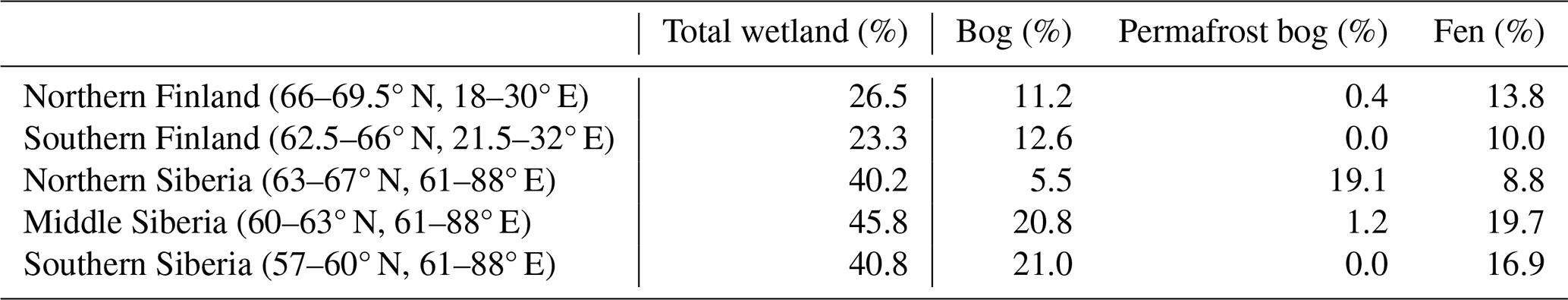
Table 1 Total wetland fraction and the three most significant wetland types in the five case study regions based on BAWLD wetland data (Olefeldt et al., 2021). In some of the regions, there are also other wetland types. Therefore, the total fraction does not necessarily match the sum of the three types listed here.

3.1 Defining the case study areas

To investigate how environmental variables explain the seasonal variability in XCH₄ over Northern Hemisphere high-latitude wetland areas, we needed to define case study regions that are both representative of wetland areas and exhibit seasonality in environmental variables. A general challenge in defining a case study area is that, on the one hand, it has to be large enough to host a sufficiently representative set of concentration observations but, on the other hand, small enough so that the area is to some extent homogeneous when considering the emissions and sinks. We tested different case study areas over Canada and Eurasia based on inversion results of natural methane fluxes (e.g. Tsuruta et al., 2023; Erkkilä et al., 2023) and wetland coverage from the Boreal–Arctic Wetland and Lake Dataset (BAWLD; Olefeldt et al., 2021). We selected five areas in northern Eurasia with sufficient spatiotemporal coverage of TROPOMI data to constrain the fit for the XCH₄ seasonal cycles and perform further analysis. The areas are shown in Fig. 1 and are called Northern Finland, Southern Finland, Northern Siberia, Middle Siberia, and Southern Siberia. The borders of the case study areas were defined based on the BAWLD dataset. Figure 1 shows the case study areas over the BAWLD total wetland fraction map. In addition, the latitude and longitude borders of the areas are listed in Table 1. The total wetland and wetland-type fractions for each case study area are also listed in Table 1. Based on the map in Fig. 1 and on Table 1, the total wetland fraction is over 40 % for the Siberian case study areas and over 20 % for the Finnish case study areas. The main wetland type is fen for Northern Finland, whereas it is bog for Southern Finland and Middle and Southern Siberia. Northern Siberia is the only area where permafrost bog is the main wetland type and also where the permafrost bog fraction is significant. The border between the Northern and Middle Siberia case study regions was defined in such a way that it separates areas where permafrost bog or bog is the dominant bog type.

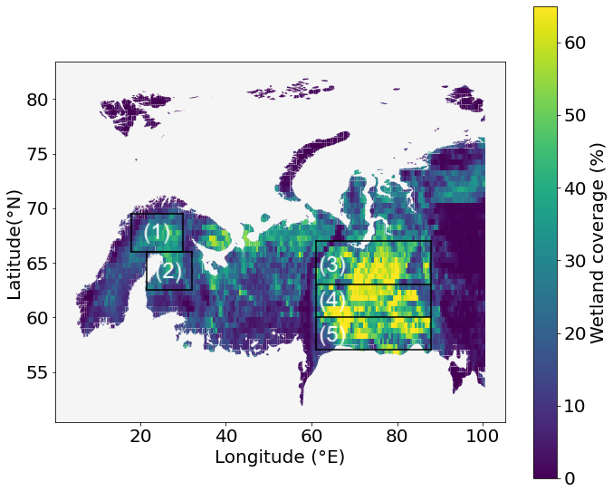
Figure 1 The Northern Finland (1), Southern Finland (2), Northern Siberia (3), Middle Siberia (4), and Southern Siberia (5) case study areas marked over the BAWLD total wetland coverage map.

3.2 Comparison of satellite-based XCH₄ to model-based XCH₄

Before applying any time series analysis, we collected all quality-flagged TROPOMI/WFMD v1.8 data for each case study region, covering the period from January 2018 to December 2023. To enable comparison between satellite-retrieved column-averaged methane and model-based estimates, each satellite observation was first co-located with the corresponding model grid cell. The modelled XCH₄ values were then calculated using the satellite averaging kernel, following the formulation by Schneising (2025):

$$\begin{array}{}\text{(1)}& {\mathrm{XCH}}_{\mathrm{4},\mathrm{mod}}=\sum _l\left(X_{\text{apr}}^l+A^l\left(X_{\text{mod}}^l-X_{\text{apr}}^l\right)\right)w^l,\end{array}$$

where A^l is the satellite averaging kernel, $X_{\text{apr}}^l$ is the prior methane profile used in the retrieval, $X_{\text{mod}}^l$ is the modelled methane profile, and w^l is the pressure-based weighting function for layer l. The modelled methane profiles were linearly interpolated from the model vertical levels to the satellite retrieval levels using the logarithm of the pressure profiles. For each day, we computed the regional daily median XCH₄ for both the satellite observations and the model estimates. Due to the relatively large grid cell size of CTE-CH₄ (6° longitude × 4° latitude) and because the WFMD prior profile is similar within each region, the modelled XCH₄ values were very similar across one region, and the variations were mainly caused by the averaging kernels of the TROPOMI/WFMD observations.

3.3 Time series gap filling and fitting of the seasonal cycle of XCH₄

After calculating the daily values, we applied a Kalman filter for gap filling the data for the fitting, and the seasonal cycle was fitted using NOAA's curve-fitting routine (CCGCRV; Thoning et al., 1989; NOAA, 2012). CCGCRV is a non-linear fitting routine developed by Thoning et al. (1989) to smooth and separate the seasonal cycle and long-term trend. CCGCRV fits the long-term trend with a third-order polynomial function, and the seasonal cycle is modelled with harmonic functions:

$$\begin{array}{}\text{(2)}& \begin{array}{rl}y=& a_{\mathrm{0}}+a_{\mathrm{1}}x+a_{\mathrm{2}}{x}^{\mathrm{2}}\\ & +\sum _{n=\mathrm{1}}^{\mathrm{4}}\left[a_{\mathrm{2}n+\mathrm{1}}\sin \left(\mathrm{2}n\mathit{\pi }x\right)+a_{\mathrm{2}n+\mathrm{2}}\cos \left(\mathrm{2}n\mathit{\pi }x\right)\right],\end{array}\end{array}$$

where the terms a₀, a₁, and a₂ represent the trend components, while the summation term captures the seasonal variation through the sine and cosine functions. The function is fitted with a linear least-squares regression routine that also gives the covariance of the fitting parameters and, therefore, the uncertainty of the parameters estimated. The fitting process produces a constant seasonal cycle, and to account for interannual and short-term variations, the residuals are filtered (NOAA, 2012; Pickers and Manning, 2015). As output, CCGCRV gives the fitted trend, harmonic seasonal cycle with no interannual variability, and smoothed seasonal cycle, where the interannual and short-term variations are included. When considering the seasonal cycle of methane, CCGCRV has been previously used, for example, to study the decreasing seasonal cycle of methane in the Northern Hemisphere high latitudes (Dowd et al., 2023) and the year-to-year anomalies of satellite observations of methane in tropical wetlands (Parker et al., 2018).

The fit for each individual day in the CCGCRV method can be described as a combination of the function fit, which represents the harmonic cycle without interannual variability, and the filtered residuals, which account for interannual and short-term variations. Similarly, the uncertainty of each component can be estimated by combining the variances of these different elements (NOAA, 2012). For example, the uncertainty of the smoothed seasonal cycle is calculated by combining the variances of the function fit and the residual filter:

$$\begin{array}{}\text{(3)}& {\mathit{\sigma }}_{\text{smooth}}^{\mathrm{2}}={\mathit{\sigma }}_{\text{function}}^{\mathrm{2}}+{\mathit{\sigma }}_{\text{filter}}^{\mathrm{2}}.\end{array}$$

Likewise, the uncertainty of the trend can be determined by combining the variances of the polynomial fit and the filter (NOAA, 2012).

Pickers and Manning (2015) investigated the possible biases related to three different curve-fitting programs, with CCGCRV being one of them. The aforementioned authors concluded and generated general recommendations on the use of these curve-fitting programs and their suitability for time series analysis. Based on these recommendations, we considered CCGCRV suitable for our analysis, as it was endorsed for cases in which the year-to-year anomalies or the magnitude or timing of the seasonal cycle are studied.

To avoid the limitations of CCGCRV related to missing observations, it was suggested by Pickers and Manning (2015) that the data are gap-filled before applying the program, as CCGCRV only interpolates over the gaps. We experimented with different gap-filling methods and studied their effect on the seasonal cycle in the Middle Siberia region. The methods tested included (1) the interpolation that CCGCRV can perform on its own and (2) Kalman filtering. For the Kalman filter, we experimented with several different parameter settings. Based on our analysis, the timing and the shape of the harmonic cycle fitted by Eq. (2) were quite similar regardless of the gap-filling method, for the time outside the winter gap in the satellite data. The main differences in the fitted cycles were related to the amplitude of the seasonal cycle, as the winter maximum often coincided with a winter data gap, and the timing of this maximum also varied slightly between fits. Based on our tests, we decided to use the Kalman filter for gap filling, as it initially provided the lowest chi-squared values for the function fit and the smallest residual standard deviation. The Kalman filter settings were further optimized to minimize the chi-squared value and the residual standard deviation, although the differences between these metrics were small and varied slightly between the model and the satellite data and between case study areas. The finalized Kalman filter configuration was kept consistent across all case study areas and for both the satellite and model datasets. For the analysis, the winter gap was excluded to avoid drawing conclusions from periods without observations.

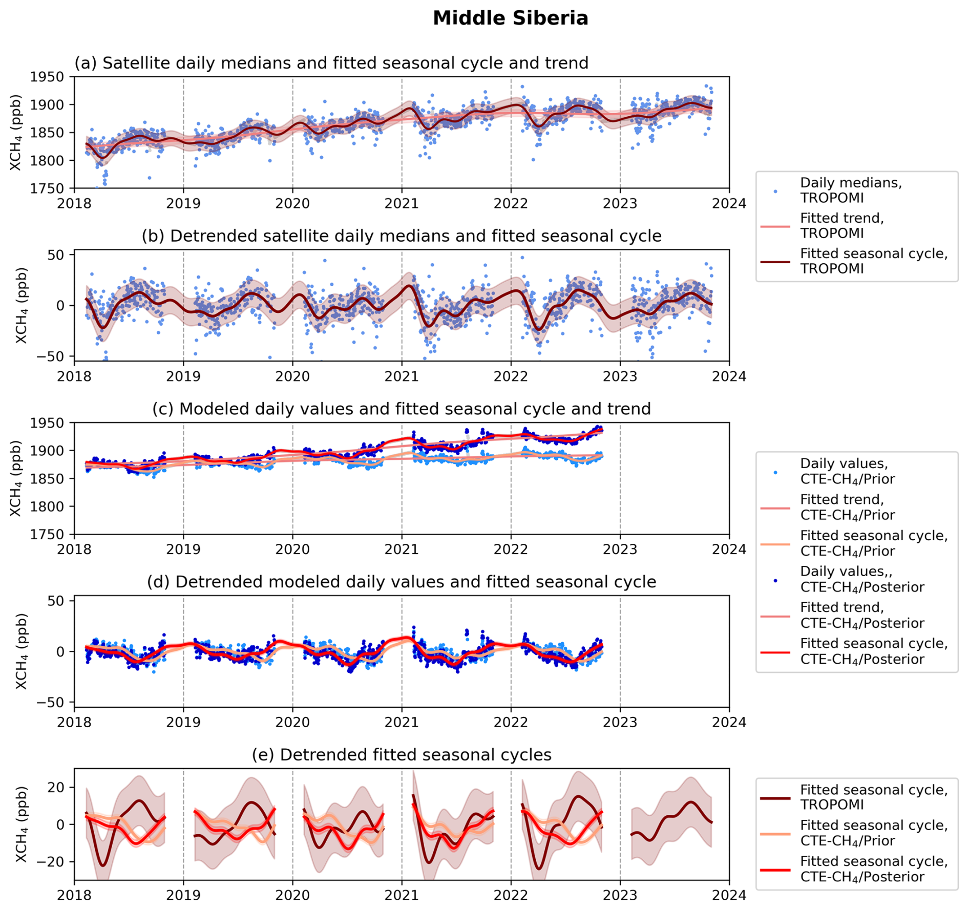
Figure 2 (a) TROPOMI/WFMD daily median XCH₄ values (blue dots) with the fitted seasonal cycle and trend, including their uncertainties (red and shaded red), for Middle Siberia. Panel (b) is the same as panel (a) but shows detrended TROPOMI/WFMD XCH₄ time series. (c) CTE-CH₄/Prior and Posterior daily XCH₄ values (lighter- and darker-blue dots, respectively), along with their fitted seasonal cycle and trend and their uncertainties (lighter- and darker-red lines and corresponding shaded areas). Panel (d) is the same as panel (c) but shows detrended CTE-CH₄ time series. (e) Detrended fitted seasonal cycles and their uncertainties for TROPOMI/WFMD and CTE-CH₄/Prior and Posterior XCH₄.

After filling data gaps using the Kalman filter, we applied CCGCRV to the gap-filled time series for each study region, both for satellite-based and model-based XCH₄. We then calculated the uncertainties associated with the smoothed seasonal cycles derived from the fitted curves. Figure 2 shows an example of the XCH₄ daily values and the fitted smoothed seasonal cycles, including their uncertainty estimates, as well as the fitted trends for Middle Siberia, based on both satellite and model data. Similar figures for other case study areas can be found in Appendix B, specifically Figs. B1–B4.

To investigate the springtime seasonal minima and maxima of the satellite-based XCH₄ seasonal cycle in relation to factors such as snowmelt, we needed to determine the dates of these minima and maxima, along with their uncertainty estimates. To calculate the uncertainty estimates, we utilized the fitted harmonic seasonal cycle and the parameters a_n provided by the CCGCRV fit (as shown in Eq. 2), along with the uncertainty estimates derived from the covariance matrix using a Monte Carlo approach. We sampled 10 000 states of the fitted cycle and calculated the dates of the minima and maxima for each state using the find_peaks function from the Python scipy.signal package. For each minimum and maximum, we computed the standard deviation across these 10 000 states and used these standard deviations as the uncertainty estimates for the results presented in Sect. 4. The distribution of the values around each individual minimum and maximum was found to be Gaussian, allowing us to use the computed standard deviation for each minimum and maximum reliably as an uncertainty estimate. This analysis was not applied to the modelled XCH₄ seasonal cycles, as their temporal behaviour did not allow for a consistent investigation of these features across regions.

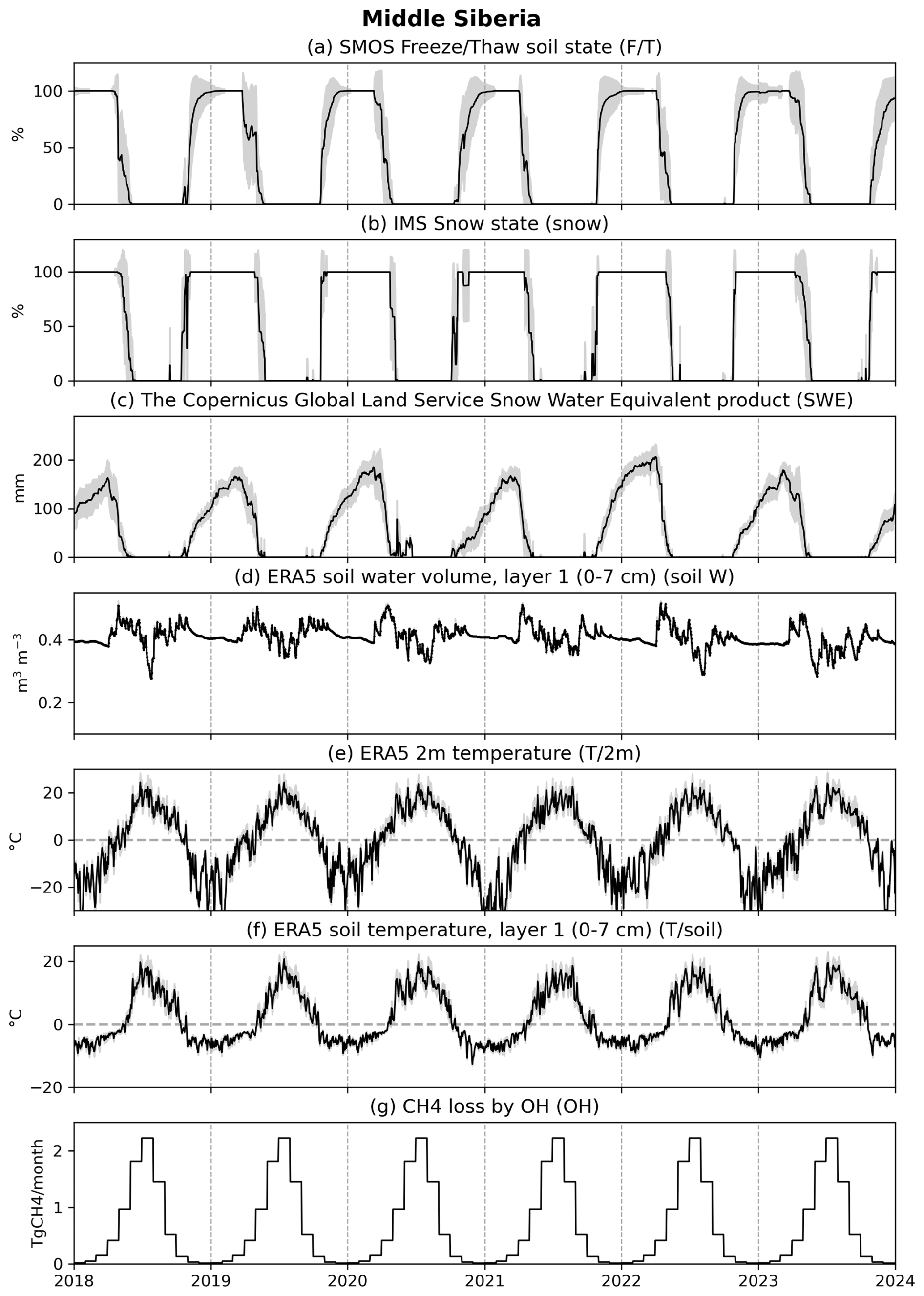
Figure 3 The black line shows the daily mean and the filled grey area shows the standard deviation of the (a) soil freeze–thaw state, (b) snow cover state, (c) snow water equivalent, (d) layer-1 soil water volume, (e) 2 m air temperature, (f) layer-1 soil temperature, and (g) CH₄ loss by OH for Middle Siberia. The abbreviation given in parentheses in the panel title is the abbreviation to be used for that environmental variable in Sects. 4 and 5.

3.4 Gridding and averaging of environmental variables

As environmental datasets in this study, we used the SMOS freeze–thaw state (F/T), IMS snow state (snow), the Copernicus Global Land Service Snow Water Equivalent product (SWE), ERA 2 m temperature (T/2m), ERA5 soil temperature at layer 1 (T/soil), ERA5 volumetric soil water at layer 1 (soil W), and CH₄ loss by OH (OH). These datasets are described in detail in Sect. 2, where, for example, the spatial and temporal resolutions are provided for each dataset. The abbreviations in parentheses correspond to the variable names used in Sect. 4.

All environmental data were initially collected for the case study areas, presented in Sect. 3.1, and daily mean values, along with their standard deviations, were calculated over the areas. There was no need to gap fill the environmental datasets, as they consist of daily time series. Variations in the temporal and spatial resolution of the datasets required slight adjustments in averaging methods. SMOS F/T and IMS snow cover are categorical datasets: SMOS F/T has three categories, whereas IMS has two. For SMOS, we defined frozen as 1, partially frozen as 0.5, and thawed soil as 0. We then averaged these values across each case study area to obtain the regional mean soil freeze–thaw state. In the IMS snow cover data, snow-covered areas were defined as 1, whereas snow-free areas were defined as a −70° N latitude band, making this consistent regardless of the study area or year. Figure 3 illustrates the environmental time series for Middle Siberia. Similar figures for other case study areas can be found in Appendix C, specifically Figs. C1–C4.

The environmental datasets have a relatively coarse spatial resolution, with the smallest grid cell size being 5 km in the SWE data and the largest being approximately 27.8 km in the ERA5 data along the longitudinal direction. The environmental variables in this case, such as snow cover or temperature, can vary significantly within these grid cells, depending on factors such as land type. For example, a transition from forest to wetland within a grid cell can lead to substantial variation in the variables. Therefore, in addition to the variability in environmental variables within the case study area, it is important to consider that there may also be variability within the grid cells.

For seasonal timing comparison (Sect. 4.2), we required estimates of the start and end dates of snow cover melt and the beginning of decreasing SWE, along with their uncertainties. We defined the start of snow cover melt as the date when the IMS snow state over the area was below 0.9, and snow cover was considered completely melted when the mean snow cover fell below 0.1. To estimate uncertainties for these dates, we examined when the mean snow cover ± 1σ uncertainty fell below 0.9 for melt onset and below 0.1 for complete melt. This approach provided uncertainty bounds in both directions for the start and end dates of snow cover melt. To obtain the date on which SWE began to decrease significantly, we normalized the SWE data for each study area for each winter and identified the first day in spring on which the normalized SWE was below 0.75; this day was used to represent the beginning of SWE decline. The uncertainties for this timing were estimated similarly to those for snow cover melt: by identifying the days when the mean SWE ± 1σ uncertainty dropped below 0.75.

3.5 Random forest feature importance and permutation importance

To study the links between the environmental variables and variability in XCH₄ on the daily level, we applied the random forest (RF) regression method, using two different importance metrics, random forest feature importance (RFFI) and permutation importance (PI), within the random forest model. Here, the environmental variables act as features in the random forest, allowing us to assess their individual contributions to XCH₄ variability. In addition, we used partial dependence plots (PDPs) to illustrate how the RF model predicts the XCH₄ concentrations as a function of a single environmental variable. PDPs can provide detailed insight into the relationship between individual environmental drivers and XCH₄.

In general, random forest is a robust and well-established ensemble learning method that averages multiple decision trees to avoid overfitting and improve accuracy (Breiman, 2001). RFFI and PI are importance metrics that can be used to evaluate the relationship between environmental variables and the seasonal variability in XCH₄. RFFI measures variable importance based on tree structure, while PI evaluates it by shuffling values within the variable, assessing the resulting impact on model performance. By analysing these scores together with PDPs, we can study the connections of environmental variables and seasonal variability in XCH₄ in more detail. The scores provide different types of information, and the calculated importance values can either support each other or highlight some differences.

The first importance method, RFFI, measures how each variable contributes to the decision-making process within the random forest model. RFFI is normalized to provide a relative ranking of variable importance so that the sum of importance values over the variables is 1. The second method, PI, describes the performance of the model when the values of each environmental variable are shuffled. PI directly measures the impact of each environmental variable on the random forest model's predictive accuracy, which provides additional information about the relevance of each environmental variable by showing how much the prediction error increases when a particular variable is disrupted. It is important to note that the calculated RFFI and PI importance values are not directly comparable, as they measure different aspects and their units are different. Using both methods together allows for a more comprehensive understanding of variable importance by comparing the effects of different importance methods and settings on the results.

Additionally, high correlations between environmental variables can influence the RFFI results, as highly correlated variables may share importance, making it difficult to distinguish their individual contributions. In contrast, PI is less sensitive to correlations, as it measures the independent impact of each variable on model performance, although it may still be affected by shared information in cases of strong correlations. For this reason, using both importance methods is advisable, as environmental variables are often correlated. The PDPs allow us to assess how each environmental variable contributes to the model's predictions. However, when interpreting PDPs, it is important to note that they may yield unrealistic results for strongly correlated variables, as the model may evaluate data combinations that do not occur in reality. Among the environmental variables that we use in our analysis, the following were highly (i.e. correlation coefficient |r|≥0.85) correlated: snow cover and snow water equivalent (r=0.89), snow cover and soil freeze–thaw state (r=0.91), snow cover and soil temperature (r = −0.85), snow water equivalent and soil freeze–thaw state (r=0.96), 2 m air temperature and soil temperature (r=0.93), and soil temperature and OH (r=0.86). These high correlations can mostly be explained by physical mechanisms and are not surprising. It is important to take these correlations into account, especially when interpreting the RFFI results or evaluating the PDPs.

The random forest model performance requires a large data volume; therefore, we collected data from all of the case study regions. For the XCH₄ satellite observations, the number of daily median values from all regions combined was 5399, whereas for the modelled XCH₄ data, the number of daily values was 4435. This difference is due to the fact that the modelled data end at the end of 2022, while the satellite time series continues until the end of 2023. The regional distribution of daily values for TROPOMI and CTE-CH₄ data, respectively, was as follows: Northern Finland, 818 and 676; Southern Finland, 820 and 675; Northern Siberia, 1201 and 993; Middle Siberia, 1218 and 1001; Southern Siberia, 1342 and 1090.

We separately studied (1) the relationship of environmental variables and the fitted seasonal cycle of XCH₄ (e.g. Fig. 2b, red line) and (2) the relationship of environmental variables and detrended daily XCH₄ values (e.g. Fig. 2b, blue dots), using both satellite and model data. The aim was to identify potentially different drivers of variability at different timescales. For both the seasonal cycle and the daily values, we used only those days on which we had TROPOMI XCH₄ observations. Therefore, the analysis and results can be considered to apply only to the spring–summer–fall period, as we are missing XCH₄ values from wintertime.

We used the scikit-learn Python module and its built-in methods and functions for fitting the model and to calculate the RFFI and PI (Pedregosa et al., 2011). The random forest model was set up with 100 decision trees and trained using 80 % of the available data, with the remaining 20 % used for testing the model's performance. The model was implemented without pruning. We tested different numbers of trees, but the model's performance did not significantly improve as the number of trees increased. Given the relatively small size of the dataset, it was important to keep the number of trees small enough. For permutation importance, we defined the number of repetitions to be 20 to obtain a robust estimate of each variable's contribution. The PDPs were also calculated using the pre-built method in scikit-learn and the brute-force approach, which generates predictions for modified input data to directly estimate the marginal effect of each variable. The brute-force method was used for its flexibility and compatibility with correlated variables and various model types.

For the results presented in Sect. 4, the number of features to consider when determining the best split (parameter “max_features”) was set to “sqrt”, meaning the number of features considered at each split was the square root of the total number of features in the model. In addition to “sqrt”, we also tested with “n_features”, where all features are considered when determining the best split. The choice of the number of features had no effect on the ranking of the feature importance, indicating robust identification of key drivers regardless of the model configuration. Model performance was assessed by calculating the coefficient of determination (R²) and root-mean-square error (RMSE) using cross-validation. For each of the three XCH₄ datasets, the R² and RMSE were slightly better with “n_features” than with “sqrt” for the seasonal cycle (e.g. for TROPOMI XCH₄, the mean R² = 0.75 ± 0.02 and RMSE = 4.33 ± 0.13 vs. R² = 0.73 ± 0.02 and RMSE = 4.50 ± 0.12 over 1000 random forest model iterations). However, for the daily medians, “sqrt” produced either better or identical metrics compared to “n_features” (e.g. for TROPOMI XCH₄, R² = 0.28 ± 0.03 and RMSE = 14.00 ± 0.37 vs. R² = 0.30 ± 0.02 and RMSE = 13.82 ± 0.37). Although the changes in performance metrics were small and the sensitivity analysis showed that the better-performing setting varied between the seasonal cycle and daily medians, “sqrt” was chosen as the final configuration because it increases tree diversity, reduces the risk of overfitting, and generally improves model generalization.

To evaluate the uncertainty of the RFFI and PI and assess the robustness of the calculated feature importance values and rankings, we performed repeated training–test splits using 1000 different random seeds and random forest model iterations. The final feature importance values presented in the results in Sect. 4 were calculated as the average across these 1000 fits, and the uncertainties of the importance values were estimated by calculating their standard deviation. In addition, PDPs, presented in Sect. 4 were computed as the mean over 1000 RF model fits, and the uncertainties are calculated by taking the standard deviation of PDPs over those 1000 fits.

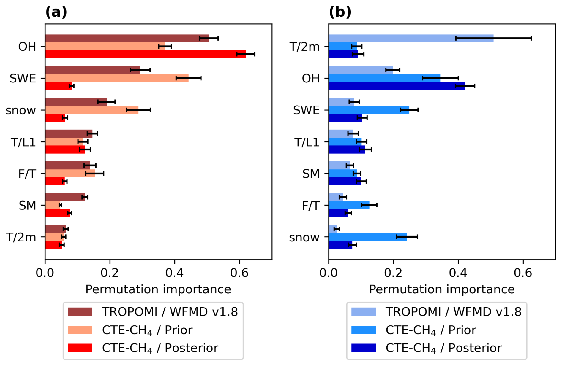
Figure 4 Permutation importance metrics for (a) XCH₄ seasonal cycles and (b) XCH₄ daily values. Different colours represent TROPOMI/WFMD, CTE-CH₄/Prior, and CTE-CH₄/Posterior. Environmental variables are ordered according to the TROPOMI/WFMD importance scores, with the most important variable at the top and the least important at the bottom. Importance values are calculated as the average of 1000 random forest model fits, and the uncertainties (black lines) represent the standard deviations across these fits.

In addition, to assess the consistency of the importance rankings, we performed a 10-fold cross-validation, repeating the entire procedure 10 times with different random seeds. The final importance scores were calculated by averaging across all folds and repetitions to obtain robust estimates. The results calculated over the ten 10-fold cross-validation runs showed similar feature rankings compared to those obtained from the 1000 random seed–based RFFI and PI results. The calculated mean importance scores were also largely consistent and fell mostly within the calculated standard deviation uncertainty ranges. Some variation was observed in individual 10-fold runs, particularly for the RFFI results, which is expected. As shown in Table A1, for example, the mean RFFI scores of four environmental variables influencing the satellite-based XCH₄ seasonal cycle fall within a narrow range of 0.11–0.13. Moreover, Fig. 4 illustrates the uncertainty ranges for the PI scores, indicating variability across the 1000 random seed iterations.

4 Results

4.1 Links between environmental variables and XCH₄

Figure 4 shows the PI scores of each of the studied environmental variables in explaining the variability in the detrended seasonal cycles of XCH₄ seasonal cycles and XCH₄ daily values. The results are shown separately for the satellite-based TROPOMI/WFMD and for the model-based CTE-CH₄/Prior and CTE-CH₄/Posterior. In addition to the visual representation in Fig. 4, Table A1 lists the mean importance scores calculated using both PI and RFFI methods over the 1000 model iterations. Table A2, on the other hand, lists the rankings of the environmental variables based on their importance scores.

Based on Fig. 4, PI indicates that OH and SWE are the two most important environmental drivers of the XCH₄ seasonal cycle for both the TROPOMI/WFMD v1.8 and CTE-CH₄/Prior dataset. For TROPOMI, OH is the most important variable, followed by SWE. For CTE-CH₄/Prior, however, SWE ranks first and OH second. These results are consistent between PI and RFFI for TROPOMI (Table A2). For environmental variables unrelated to snow, the ranking varies substantially more between PI and RFFI in both TROPOMI and CTE-CH₄/Prior, although the importance scores of these variables are generally similar (Table A1). In contrast, the importance scores and rankings for the CTE-CH₄/Posterior dataset differ markedly from those of the other two XCH₄ seasonal cycles. OH is clearly the dominant driver in this case, while all other variables exhibit significantly lower importance scores, particularly in the PI results where the separation between OH and other variables is the most pronounced. The consistency of these findings is further supported by the overall performance of the random forest models. The mean coefficient of determination (R²) for the XCH₄ seasonal cycle is 0.73 for TROPOMI/WFMD, 0.89 for CTE-CH₄/Prior, and 0.84 for CTE-CH₄/Posterior. This indicates that seasonal variability is captured by the environmental variables selected in the three datasets.

For the daily values of XCH₄, both CTE-CH₄/Prior and CTE-CH₄/Posterior show that OH is the most important variable according to the PI. However, for TROPOMI/WFMD, air temperature is the most important driver. Despite the relatively wide uncertainty range associated with air temperature (Fig. 4), its dominant role is clearly evident and further supported by the RFFI (Table A2). The ranking of environmental variables varies considerably between the PI and RFFI for both CTE-CH₄/Prior and CTE-CH₄/Posterior. For example, while the PI identifies OH as the most important driver in the CTE-CH₄/Prior case, the RFFI ranks OH only sixth. Nevertheless, the mean coefficient of determination (R²) for the XCH₄ daily values is 0.30 for TROPOMI/WFMD, 0.59 for CTE-CH₄/Prior, and 0.51 for CTE-CH₄/Posterior. These values are notably lower than those for the XCH₄ seasonal cycle.

Figure 5 presents PDPs of the detrended seasonal cycle of XCH₄, showing the modelled response of XCH₄ seasonal variability to changes in each environmental variable. The results are shown separately for TROPOMI/WFMD, CTE-CH₄/Prior, and CTE-CH₄/Posterior. Figure 6 shows the corresponding PDPs for the detrended daily values of XCH₄. A decreasing line in the PDPs indicates that the RF model predicts lower XCH₄ values as the environmental variable increases. Conversely, an increasing line suggests that XCH₄ increases with the environmental variable. A steady line implies minimal dependency between the variable and the modelled XCH₄ response. When analysing the PDPs, it is important to focus on the shape and trends of the curves rather than absolute values, as these plots should be used to illustrate relative dependencies rather than quantitative predictions.

Figure 5 Partial dependence plots of the seasonal cycle of XCH₄. The red lines show the average RF model response to each environmental variable, calculated over 1000 RF fits. Shaded areas represent the standard deviation across RF model runs, indicating the uncertainty of the partial dependence. The results are shown for three data sources (TROPOMI/WFMD, CTE-CH₄/Prior, and CTE-CH₄/Posterior), each plotted in different shades of red, with their corresponding uncertainties shown as shaded areas. Panels illustrate the modelled partial dependence of the XCH₄ seasonal cycle on the (a) soil freeze–thaw state (F/T), (b) snow cover (snow), (c) snow water equivalent (SWE), (d) layer-1 soil moisture (SM), (e) 2 m air temperature (T/2m), (f) layer-1 soil temperature (T/L1), and (g) CH₄ loss by OH (OH).

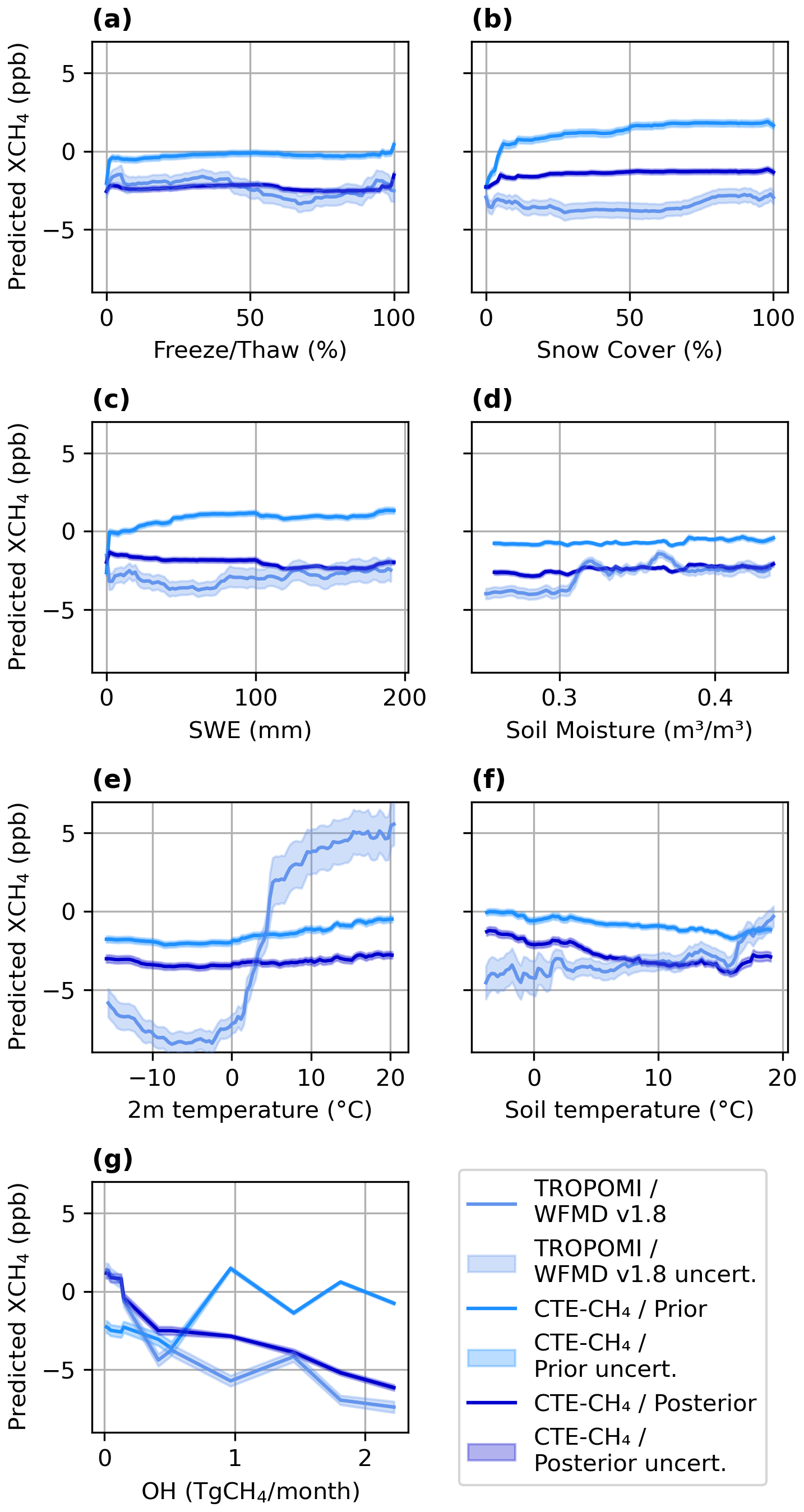
Figure 6 Partial dependence plots of the daily values of XCH₄. The blue lines show the average RF model response to each environmental variable, calculated over 1000 RF fits. Shaded areas represent the standard deviation across RF model runs, indicating the uncertainty of the partial dependence. The results are shown for three data sources (TROPOMI/WFMD, CTE-CH₄/Prior, and CTE-CH₄/Posterior), each plotted using different shades of blue, with their corresponding uncertainties shown as shaded areas. Panels illustrate the modelled partial dependence of XCH₄ daily values on the (a) soil freeze–thaw state (F/T), (b) snow cover (snow), (c) snow water equivalent (SWE), (d) layer-1 soil moisture (SM), (e) 2 m air temperature (T/2m), (f) layer-1 soil temperature (T/L1), and (g) CH₄ loss by OH (OH).

Overall, the partial dependence of TROPOMI/WFMD XCH₄ on the studied variables is closer to the dependence of CTE-CH₄/Posterior XCH₄ compared to CTE-CH₄/Prior. The partial dependence of the seasonal cycle is the strongest for OH: OH exhibits a consistent negative relationship with XCH₄ for TROPOMI/WFMD and CTE-CH₄/Posterior. In contrast, the response of CTE-CH₄/Prior is more irregular and even anti-correlated with the predicted TROPOMI/WFMD XCH₄. The XCH₄ daily values have similar partial dependence on OH to the seasonal cycle; however, for TROPOMI/WFMD XCH₄, air temperature has the most pronounced marginal effect. The model predicts a strong increase in XCH₄ as air temperature rises from 0 °C to approximately 5 °C, after which the response continues to increase but at a lower rate. For the model-based daily values, the partial dependence on air temperature, as well as other variables, is relatively flat and indicates a minimal marginal effect. In addition to air temperature, the dependence on soil temperature in the model-based values, both seasonal cycle and daily, is opposite in direction compared to the satellite-based case. For TROPOMI/WFMD, the response is positive, indicating that higher soil temperatures are associated with increased XCH₄. In contrast, both CTE-CH₄/Prior and Posterior exhibit a negative dependence, suggesting a divergent behaviour between satellite-based and model-based seasonal cycles.

Snow water equivalent shows a strong relationship with the TROPOMI-based XCH₄ seasonal cycle for SWE values below 50 mm, after which the response flattens. For CTE-CH₄/Prior, the relationship with SWE is increasing, such that higher SWE values are associated with higher XCH₄ values, while CTE-CH₄/Posterior shows slight decreasing trend, similar to TROPOMI/WFMD. For TROPOMI/WFMD and CTE-CH₄/Prior, snow cover shows similar pattern to SWE, but it is almost flat for CTE-CH₄/Posterior.

In addition to seasonal cycles and daily values, we tested the capability of the RF model to predict the daily value–seasonal cycle difference. The coefficient of determination (R²) for this difference was between 0.11 and 0.13 for all three datasets, indicating that only slightly over 10 % of the variability in the difference could be explained with the RF model. As the R² values were this low, we did not perform an importance score analysis. While such an analysis could have indicated which of the environmental variables had the most significant contribution to the explained 10 %, the overall explained variability was considered too limited for a meaningful interpretation. The mean daily value–seasonal cycle difference varied between case study areas: for TROPOMI/WFMD, the range was −0.43 to 0.29 ppb; for CTE-CH₄/Prior, it was −0.04 to 0.9 ppb; and for CTE-CH₄/Posterior, it was −0.01 to 0.16 ppb.

4.2 Seasonal timing of XCH₄ minima and maxima in relation to snow

Our results in Sect. 4.1 demonstrate that snow-related variables, specifically snow water equivalent and snow cover, influence the seasonal cycle of satellite-based XCH₄. To further investigate the temporal connection between snow and the seasonal cycle of XCH₄, we focused on spring, particularly on the minimum XCH₄ in early spring and the local maxima in late spring or early summer, coinciding with snowmelt. We focused on spring and not on the annual maximum, as the annual maximum often coincides with a time when TROPOMI observations are not possible, due to polar night or low solar elevation (e.g. Fig. 2; see data gaps in winter 2021 and 2022). Additionally, the onset of snow cover frequently occurs during this period (Fig. D1), further complicating late-autumn or early-winter analyses. For the analysis, we defined the end of snowmelt based on snow cover, rather than SWE, because it is a simpler method for determination, and in SWE time series, it is observed that significant amounts of snow may still fall after SWE approaches zero, for example, in Fig. 3c in the spring of 2020. When determining the end of snowmelt based on snow cover, these situations were more precisely defined. The onset of snowmelt, however, must be defined through the start of SWE reduction, as SWE begins to decrease much earlier than snow cover (Fig. D1), i.e. snowpack begins to melt from the top before the ground becomes completely snow-free. Threshold-based methods for defining the onset and end of snowmelt are described in Sect. 3.4.

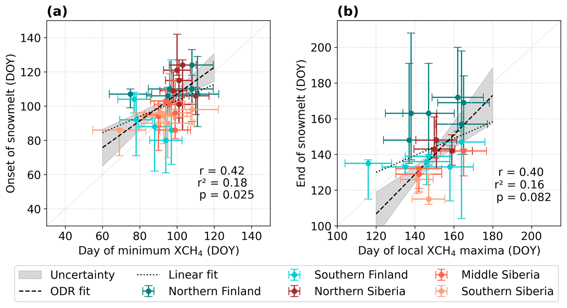
Figure 7 Scatterplots show (a) the onset of snowmelt (y axis) vs. the day of the year on which the XCH₄ seasonal cycle reaches its minimum (x axis) and (b) the end of snowmelt (y axis) vs. the day of the local maxima in XCH₄ (x axis). Both panels also display the one-to-one line (grey dots), a linear fit (dotted black line), and an orthogonal distance regression (ODR) fit (dashed black line). The ODR fit accounts for uncertainties in both directions, with all uncertainties calculated based on the data. Additionally, the panels display the Pearson correlation coefficient (r), the coefficient of determination (R²), and the corresponding p value.

The seasonal cycle of XCH₄ generally reaches its minimum in early spring and its maximum during autumn or winter. In some years, particularly in the Finnish case study areas, local minima and maxima in XCH₄ are observed during late spring, often coinciding with snowmelt (Fig. D1). Figure 7a shows the day of minimum XCH₄ relative to the onset of snowmelt, whereas Fig. 7b presents the day of a local maximum in XCH₄ compared to the end of snowmelt. In Fig. 7a, the 2023 data point for Southern Finland is excluded because the XCH₄ minimum falls at the edge of the TROPOMI time series and is, therefore, not considered reliable. Both panels include a linear fit, represented by a dotted line, and an orthogonal distance regression (ODR) fit, indicated by a dashed line. The ODR approach accounts for uncertainties in both the x and y directions. Both figures also display the Pearson correlation coefficient (r), the coefficient of determination (R²), and the corresponding p value. Uncertainties related to the timing of snowmelt and the phase of the XCH₄ seasonal cycle are calculated as presented in detail in Sects. 3.3 and 3.4.

Based on Fig. 7a, the onset of snowmelt shows a moderate positive correlation with the timing of the XCH₄ seasonal minimum, within uncertainties. When the potential outlier from the Southern Finland case study area in 2023 is excluded, as discussed earlier, the Pearson correlation coefficient (r) is 0.42. Including the outlier reduces the correlation to 0.32, highlighting the sensitivity of the result to individual data points given the small sample size (N=30, covering 6 years and five case study areas). Nevertheless, with a p value below 0.05, the relationship can be considered statistically significant, indicating a non-random association between snowmelt onset and XCH₄ minimum timing. In contrast, the correlation between the timing of the local XCH₄ maximum and the end of snowmelt is slightly weaker, with a Pearson correlation coefficient of 0.40. However, the associated p value of 0.082 indicates that this relationship is not statistically significant at the 0.05 threshold. This analysis is further constrained by a smaller number of observations (N=20; Fig. D1), increasing the influence of individual data points on the statistical outcome. The relationship between the XCH₄ phase and snowmelt timing appears to be clearest in the Finnish case study areas, where a local maximum of XCH₄ occurs in conjunction with snowmelt in every year studied. In Northern and Middle Siberia, this pattern is observed in 3 years, whereas it is observed in 2 years in Southern Siberia, but the local maximum is less distinct in the latter region compared with the Finnish areas. However, in Southern Siberia, even in those 2 years, the timing of the local XCH₄ maximum does not align with the end of snowmelt. In both cases, the slopes of the ODR and linear fits differ similarly, reflecting the influence of the uncertainty distribution and potential outliers. Overall, the ODR fits indicate that the onset of snowmelt tends to occur after the XCH₄ minimum, while the local XCH₄ maximum generally follows the end of snowmelt.

5 Discussion

5.1 Links between environmental variables and XCH₄

The driving factors and conditions of the seasonal variability in methane emissions from different land and vegetation types have previously been widely studied with in situ measurements as well as modelled CH₄ fluxes and concentrations. As stated in Sect. 1, the seasonal variability in the column-averaged dry-air mole fraction of methane is a combination of the seasonality in CH₄ emissions and sinks and in atmospheric transport patterns. Therefore, the results from local flux studies cannot be directly compared to our findings, although fluxes influence the observed XCH₄ concentrations.

Next, we compare our results with previous findings from in situ measurements and modelling studies and examine how the dependencies of methane on environmental variables identified in those studies are reflected by our results. We will also discuss key differences between satellite and model-based results, with the aim of identifying similar patterns and discrepancies as well as the possible reasons behind them. The comparison against CTE-CH₄/Prior concentrations provides insight into how well the prior fluxes, especially process-model-based wetland CH₄ fluxes, which are expected to be the main driver of the flux seasonality in the study regions, can reproduce the observed seasonal variability in total-column methane and its dependence on environmental drivers. In contrast, the posterior results assess the capability of surface-based inversion simulation to optimize and capture key features of the total column. In the inversion simulations, surface observations are used to optimize the posterior fluxes so that the model reproduces the observed surface concentrations. XCH₄ is then calculated from the modelled concentrations using these fluxes, and since part of the column variability originates higher in the atmosphere, the resulting total-column values can differ substantially from satellite-based XCH₄.

Role of the OH sink

East et al. (2024) studied the hemispheric differences and the drivers of the seasonality in methane concentrations based on model simulations. They showed that the seasonal cycle in the Southern Hemisphere is smooth and primarily driven by the OH sink, whereas the cycle in the Northern Hemisphere is asymmetric and exhibits a sharp increase during summer. Based on their chemical transport model results, they concluded that, in addition to the role of OH, the magnitude, latitudinal distribution, and seasonality of wetland emissions are critical factors influencing the seasonal cycle of methane in the Northern Hemisphere, as they determine the timing and magnitude of the summer increase. In our results, OH was identified as the most significant factor for the TROPOMI/WFMD and CTE-CH₄/Posterior XCH₄ seasonal cycles, based on both the PI and RFFI scores. This finding is consistent with East et al. (2024) and demonstrates that, for total-column methane, atmospheric CH₄ loss is one of the key drivers of seasonal variability. For the CTE-CH₄/Prior seasonal cycle, OH was the second most important factor. For daily values, there was a clear difference between satellite-based and model-based results, as both CTE-CH₄/Prior and Posterior ranked OH as the most important variable, whereas OH was clearly less important for satellite data. For satellite daily medians, there was a difference in the OH rankings between the PI and RFFI, but this may be due to the high correlation between OH and soil temperature (r=0.87). For TROPOMI/WFMD and CTE-CH₄/Posterior XCH₄, the partial dependencies showed a pattern that we expected based on East et al. (2024): as OH (i.e. CH₄ loss by OH) increases, the predicted XCH₄ decreases. The observed non-smooth pattern in PDPs is a result of the monthly resolution of the OH data used. For the model-based results, the significant role of OH in determining XCH₄ is, to some extent, expected, as a similar method (Sect.2.7) for representing the OH sink is applied in the CTE-CH₄ model (Sect.2.2).

The method used to describe the effectiveness of the OH sink is a simplification, as we assumed that large-scale OH loss, monthly zonal mean CH₄ loss values calculated for the 57–70° N latitude band, is sufficient to examine the variability in XCH₄ in this study. This is based on the assumption that OH loss does not vary significantly between the study areas at a monthly resolution. However, this assumption does not account for the fact that OH concentrations depend on factors such as UV radiation and humidity (Lelieveld et al., 2016; Zhao et al., 2019) and that reaction rates with CH₄ depend on air temperature and, thus, exhibit shorter-term and interannual variability. This might be one reason why OH had less impact on the daily variability in satellite-based XCH₄ than in the seasonal cycle. As we focus on Northern Hemisphere high latitudes, we are dealing with surfaces that are both spectrally and seasonally variable, particularly due to snow cover, which can influence OH levels via changing UV reflectivity. For instance, Prinn et al. (2001) showed that, during El Niño–Southern Oscillation (ENSO) events, increased cloud cover corresponds to reduced OH concentrations, likely due to decreased near-surface UV radiation. Consequently, snow cover may impact not only methane fluxes but also the atmospheric methane sink indirectly. Studying the effectiveness of the OH sink in more detail would require more accurate OH estimates or the use of new proxies that can capture small-scale spatiotemporal variability. Given that the lifetime of OH is extremely short (typically around 1 s) and that it is highly sensitive to perturbations in both its sources and sinks (Wolfe et al., 2019), it is challenging to measure OH directly or to model its spatial variability reliably. Until now, atmospheric methyl chloroform concentrations have often been used as a proxy for OH; however, this approach is becoming increasingly difficult as methyl chloroform levels decline (Zhang et al., 2018).

Role of snow conditions and frozen ground

Snow and frost require similar conditions, specifically temperatures below 0 °C. Moreover, they are closely interconnected: snow acts as an insulating layer, influencing soil freezing and thawing. For methane emissions, snow plays an important role, as it hinders methane from entering the atmosphere from the soil. Snow also contributes to soil thawing, as water from melted snow thaws the soil from above and increases the soil water volume. Studies that have carried out measurements outside of the growing season have mainly focused on quantifying fluxes during the cold season and comparing them to annual emissions. However, only few studies have directly studied the relationship between snow and methane fluxes, partly due to the difficulty in accessing in situ observation sites during the winter months. The cold-season emissions can cover a major part of the annual emissions, despite snow and soil frost (e.g. Zona et al., 2015; Rößger et al., 2022). The emissions during the cold season are relatively stable, with a monthly distribution accounting for 4 %–8 % of the annual emissions (Rößger et al., 2022). However, as the cold season lasts from early October to early May in some parts of the high latitudes, a significant amount of emissions is accumulated over this time period; therefore, the cold-season emissions are important to the annual methane budget in these areas. As mentioned in Sect. 2.5, the quality of SMOS F/T product data near Russia is affected by RFI interference. However, in our case, it was observed that the interference significantly impacted the data quality only for the year 2023. Our earlier results, which did not yet include data from 2023, were consistent with the current findings. This consistency suggests that the interference has not impacted our results, which is logical given the relatively low importance of soil freezing (Fig. 4).

From studies that have directly investigated the connections between snow and methane, Mastepanov et al. (2013) found that the springtime increase in the CH₄ flux was strongly correlated with the timing of snowmelt. Additionally, Rößger et al. (2022) reported that earlier snowmelt and higher early-summer temperatures in June have increased the early-summer CH₄ fluxes in Siberian tundra. Both Zona et al. (2015) and Rößger et al. (2022) showed a significant rise in methane emissions over a wetland following the spring thaw, followed by strong monthly emissions that lasted over the thaw season. They both defined the seasons based on temperatures, either air or soil.

Our results show that, for the seasonal cycle, especially for the satellite-based XCH₄, snow is a more important determining factor than for the XCH₄ daily medians; the amount and coverage of snow help determine the phase of the XCH₄ seasonal cycle along with OH. For the TROPOMI/WFMD seasonal cycle of XCH₄, the partial dependence of SWE and snow cover (Fig. 5b and c) behaves as expected based on Zona et al. (2015) and Rößger et al. (2022): when the snow is melting or close to melting, XCH₄ increases. This pattern is visible in the seasonal cycle PDPs, whereas the curves for daily medians are flatter (Fig. 6b and c). For CTE-CH₄/Posterior, the snow-related partial dependence curves are nearly flat, which is as expected, since OH was clearly more important for the seasonal cycle than other environmental variables. For CTE-CH₄/Prior, however, the snow-related environmental variables do not behave as expected: for daily values, the curves are nearly flat, whereas for the seasonal cycle, they show an increase in XCH₄ with increasing snow, which would imply higher methane concentrations in the presence of snow than without it. This possibly indicates inaccuracy of the LPX-Bern DYPTOP process-based model with respect to estimating CH₄ fluxes under snow conditions.

Mastepanov et al. (2013) and Rößger et al. (2022) examined the effects of snow on small, well-defined land cover types, whereas in our study, the SWE data resolution is 5 km, approximately the same as the TROPOMI pixel size. Despite this relatively fine resolution, it still encompasses a mixture of land cover types with varying snowmelt timings. In addition, when averaging across the entire case study area, further variability arises due to the diverse land cover types present. As listed in Table 1, none of the areas had a total wetland fraction exceeding 50 %, indicating that more than half of the area consists of non-wetland types.

For the model results, the significance of snow in the CTE-CH₄/Prior seasonal cycle of XCH₄ is somewhat surprising, as the prior fluxes are monthly and do not account for the exact annual timing of snowmelt or detailed snow cover information. Moreover, since the partial dependence behaviour of snow-related variables is also not as expected, it is possible that other processes or correlations are confounded with snow in the CTE-CH₄/Prior results. The comparison between satellite and model-based results suggests that the agreement in variable importance could be improved if the calculation of prior fluxes incorporated more detailed, year-specific information on snow cover and melt timing, as snow and its melting appears to play a clearly more important role in the seasonal cycle of XCH₄ based on satellite observations.

Role of air and soil temperature and soil moisture

Based on flux studies, it can be stated that there is a positive correlation between methane flux and soil temperature during the growing season (e.g. Mastepanov et al., 2013; Howard et al., 2020; Kittler et al., 2017). This relationship is linked to microbiological activity, which is enhanced by higher soil temperatures, leading to increased methane emissions from wetlands. Zona et al. (2015) showed that CH₄ emissions are small when the soil temperature is below 0 °C, but as the soil temperature increases toward 0 °C and above, methane emissions begin to rise, with the highest emissions occurring during July and August. Similarly, Kittler et al. (2017) showed that emissions peak during July and August and follow the soil temperature.

According to both the PI and RFFI scores, air temperature is the most important factor influencing the detrended satellite-based XCH₄ daily medians, although the uncertainty range for the PI is relatively high. Nevertheless, air temperature remains clearly the most important variable within this range. The partial dependence plot (Fig. 6e) shows that the predicted XCH₄ starts to increase sharply when the air temperature approaches 2 °C, which is theoretically in line with Zona et al. (2015) and Kittler et al. (2017), although in our case the variable is air temperature, not directly the soil temperature. When interpreting PDPs, it must be noted that strongly correlated variables may lead to shared attribution in the PDPs, and the correlation between air temperature and soil temperature was high (r=0.93). Nonetheless, soil temperature (Fig. 6f) exhibits a similar trend, although clearly weaker; i.e. as temperature increases, the predicted XCH₄ also increases. This is consistent with the hypothesis that rising temperatures enhance methane emissions, which should in turn be reflected as an increase in total-column methane. In addition, the importance of air temperature may also reflect the influence of dynamical weather events on the daily variability in XCH₄. However, as the explanatory power of the RF model for TROPOMI/WFMD daily medians was relatively low (R² = 0.32), we cannot conclude that daily variability in XCH₄ is driven by temperature alone, since only approximately one-third of the variability can be explained by the model.

The CTE-CH₄/Prior and CTE-CH₄/Posterior results mainly show a weak dependence on temperature. For the seasonal cycle, CTE-CH₄/Prior displays a slight increase at the highest air temperatures, while for soil temperature, both versions show a decreasing trend, which is opposite to that observed in the satellite data and expected based on in situ studies. For daily values, both model versions show a slightly increasing trend with air temperature but a decreasing trend with soil temperature. Taken together, the importance scores and partial dependence plots suggest that the modelled XCH₄ responds less strongly to temperature variations compared to the satellite-based results and that it does not reflect short-term fluctuations in temperature between days. This is at least partly expected, as day-to-day variability is considerably lower in the model than in the satellite data (e.g. Fig. 2b and d).

The effect of soil moisture on methane emissions is complex, and the process is significantly influenced by factors such as wetland type or the time period (month, season, or year) being studied. For example, Kittler et al. (2017) compared methane emissions from a drained area to a moister control area on moist tussock tundra that is located on a Siberian permafrost area. They showed that the annual amount of methane emissions is correlated with soil moisture; in the drained area, annual methane emissions were lower than in the moister control areas. On the other hand, Zona et al. (2015) studied emissions from the Alaskan tundra and showed that, at the driest sites, cold-season emissions dominated the annual emissions. Our results do not indicate a systematic impact of soil moisture on XCH₄ variability, as the ranking of soil water volume varies between satellite-based and model-based data and seasonal cycle and daily values (Table A2). In addition, the importance scores of soil moisture are generally low (Table A1).

The lack of a systematic response may arise from relatively strong day-to-day variability in soil moisture during the summer as well as significant local variations, such as differences in soil types (e.g. Kittler et al., 2017, and their comparison between two adjacent areas). Aalto et al. (2025) studied how process-based ecosystem models responded to air temperature and precipitation in Fennoscandia. They found that models with a more pronounced peatland component were more temperature-driven, whereas models with a more pronounced wet mineral soil component were more precipitation-driven. The CTE-CH₄ posterior wetland emissions, based on fluxes from two models with contrasting response patterns, depended on both air temperature and precipitation. In addition, Hyvärinen et al. (2025) found that, when large-scale methane emissions were studied, the process-model-based methane emissions increased when the snow melted and the soil thawed, and at the same time, the air temperature rose above 0 °C. They also observed a peak in methane fluxes caused by an inundation component, potentially brought about by melted snow. Since the environmental variables used in this study are relatively sparse with respect to the spatial grid resolution and are then averaged over larger areas, there are inevitably many different land cover and wetland types within each grid cell and within the case study area. To study the effect of soil moisture on XCH₄ at a more detailed level, it would likely be necessary to consider different soil types individually, permafrost areas, and the relationship between soil moisture and individual XCH₄ satellite observations. We tested the analysis using satellite-based soil moisture data (Dorigo et al., 2017); however, these are not daily data, and there were significant data gaps during springtime. This prevented a comprehensive satellite-based analysis and was the reason that we used ERA5 soil water volume instead.

Synthesis of satellite and model results

The similarities and discrepancies between the PI and RFFI scores and the PDPs suggest that, for the TROPOMI/WFMD XCH₄ seasonal cycle, the RF model performs relatively consistently. OH and SWE emerge as the main drivers of the seasonal cycle, and their influence aligns with physical expectations based on in situ observations. The robustness of the results is further supported by the high explanatory power of the model, as indicated by the coefficient of determination for the seasonal cycle (R² = 0.73), showing that the model captures most of the seasonal variability. However, for the satellite-based short-term XCH₄ variability, the RF model is less stable, indicating that the mechanisms explaining daily variability are more complex and that short-term environmental variability has little systematic impact on the total column, which is reasonable. This is reflected by the lower coefficient of determination (R² = 0.32). Nonetheless, our results on the effect and importance of temperature are consistent with in situ studies that demonstrate the role of temperature in driving methane variability.

We expected differences between the satellite and model-based results, as it has been shown that the CTE-CH₄ model, and inversion models in general, estimate global total emissions well, while regional estimates are strongly dependent on the prior emission datasets used (e.g. Tenkanen et al., 2025). In our analysis, we used surface-observation-based posterior results, meaning that the posterior fluxes are optimized to match surface methane concentrations. However, part of the XCH₄ variability originates in the upper atmosphere. For example, the OH sink is not specifically located near the surface (Saunois et al., 2025). Moreover, in the optimization, there was a difference between 2018–2021 and 2022: for 2022, no surface observations were available from Russia, which covers a large part of the high-latitude region.

Generally, we found that the environmental variables had a stronger and more consistent effect on TROPOMI/WFMD and CTE-CH₄/Posterior than on CTE-CH₄/Prior. Furthermore, the mechanisms through which environmental variables influenced the total-column concentrations were better explained and more coherent for TROPOMI/WFMD and CTE-CH₄/Posterior than for the Prior. For example, increasing OH sink led to a decreasing response in total-column methane for both TROPOMI/WFMD and CTE-CH₄/Posterior, whereas the response was irregular and even increasing for CTE-CH₄/Prior. This decreasing response is expected, as the OH sink is the main removal process of methane in the atmosphere. The effect of snow was fairly weak in CTE-CH₄/Posterior, while for TROPOMI/WFMD, a decreasing amount of snow corresponded to the increasing phase of the XCH₄ seasonal cycle; i.e. when snow melts, methane increases. In contrast, for CTE-CH₄/Prior, the seasonal cycle increased with increasing snow amount and coverage, which is not consistent with expectations based on in situ results. It should be noted that these results apply only to spring, as our time series was limited by the winter gap in satellite observations. If winter periods had been included, they would have required a separate analysis, although it remains unclear how XCH₄ behaves during winter in high Northern Hemisphere latitudes. During this period, wetland emissions are minimal, and the OH sink is also weak due to the absence or low level of sunlight. Therefore, no conclusions can be drawn regarding winter conditions, and the results presented here apply exclusively to the spring–summer period.

The time series of CTE-CH₄/Prior, CTE-CH₄/Posterior, and TROPOMI/WFMD showed that the background level of total-column methane concentrations differs between datasets (e.g. Fig. 2a and c), with the model consistently overestimating XCH₄ across regions and years. This feature has been previously noted by Tsuruta et al. (2023), and potential causes include vertical transport (stratosphere–troposphere exchange), atmospheric chemistry, tropopause height estimation, and model resolution in both the horizontal and vertical directions (Tsuruta et al., 2025, 2023). These may also contribute to the differences in environmental variable importance for the model-based seasonal cycles: for CTE-CH₄/Prior, snow amount was found to be the most important variable and OH sink the second, whereas for CTE-CH₄/Posterior, the OH sink was clearly dominant, with other environmental variables being much less important and having only small differences between them. It seems that, when optimizing the posterior fluxes, the model tries to produce the seasonality of the sinks rather than the sources. In addition, since we used a surface-data-based inversion, the model does not necessary aim to match the total column concentrations, which have different phases in seasonal cycles (e.g. Tsuruta et al., 2023).

The transport model was run at a relatively coarse spatial resolution of 6° × 4°, which corresponds to roughly 200–350 km in the west–east direction and nearly 450 km in the south–north direction. Compared to the TROPOMI pixel size, the model grid cell area is over 2000 times larger, and each grid cell contains a wide range of land cover types and environmental conditions. The same applies to our case study areas, which also exhibit considerable variation in land cover and environmental conditions. For the satellite data, we used the daily median to reduce the influence of within-area variability, so that each daily median represents a central estimate across the region. In addition, as discussed earlier, day-to-day variability is significantly higher in the satellite observations than in the model, which is expected, since the modelled daily concentrations are based on weekly posterior fluxes and monthly prior fluxes, making it challenging to capture finer temporal dynamics.

Generally, our satellite-based findings support the results of East et al. (2024), who used multiple chemical transport model simulations and found that the magnitude, latitudinal distribution, and seasonality of wetland emissions are critical for the methane seasonal cycle in the Northern Hemisphere, as they determine the timing and magnitude of the summer increase. Our results highlight the importance of OH and further specify this relationship between the seasonal cycle and wetland emissions by demonstrating that environmental variables directly linked to wetland emissions, such as temperature and SWE, including water from snowmelt, are key factors for methane production in high-latitude wetlands, either directly or indirectly, by influencing the soil water cycle and soil temperature.

5.2 Seasonal timing of XCH₄ minima and maxima in relation to snow

Snow influences wetland methane emissions in multiple ways; for instance, it acts as an insulating layer for the soil, affecting soil temperatures and freezing processes, thereby directly impacting methane production in the soil. Snow also hinders methane emissions entering the atmosphere from the soil. In spring, as snow melts, a pulse of methane emissions is often observed, resulting from methane that accumulated beneath the snow and ice during winter being released after the snowmelt and soil melt (Rinne et al., 2007). Additionally, soil moisture is closely linked to snowmelt in spring; Figs. C3, 3, and C4 show that the soil water volume in the Siberian case study areas typically increases sharply to a distinct peak during the period between the onset and the end of snowmelt. This increase in soil water volume is linked directly to melting snow. In Northern and Southern Finland, this pattern is less distinct, although similar features can still be observed to some extent (Figs. C1 and C2).

In situ and modelling studies have mainly focused on the effect of soil freeze and thaw on methane emissions rather than on the impact of snow (e.g. Bao et al., 2021; Tenkanen et al., 2021). Based on previous studies, we were not able to draw clear conclusions regarding whether the coincidence between the onset of snowmelt and the day of minimum XCH₄ is due to a relationship between the two. This uncertainty originates from limited knowledge about the amount of methane released during the early stages of snowmelt, when snow cover persists and the soil may still be frozen.

The possible correlation between the day of local maxima in XCH₄ and the end of snowmelt may be related to the known connections between snow and methane, as discussed in Sect. 5.1. For example, Mastepanov et al. (2013) showed a strong correlation between the springtime increase in CH₄ and the timing of snowmelt, while Rinne et al. (2007) observed an emission pulse during intense melting. However, in our analysis, the correlation between the day of local maxima in XCH₄ and the end of snowmelt was not statistically significant, likely due to the limited number of observation points. Further analysis of this potential relationship would require a larger dataset to either prove or disprove this hypothesis.

Bao et al. (2021) showed that the hourly mean emissions during spring thaw are lower than those during autumn freeze at high-latitude tundra sites. Additionally, the mean duration of spring thaw is typically less than 1 month (Hyvärinen et al., 2025), whereas autumn freeze lasts nearly 2 months (Erkkilä et al., 2023). Since our analysis suggests that spring snowmelt may influence the seasonal cycle of XCH₄, it is reasonable to expect that the impact of autumn snow onset or soil freeze could also be detectable if we had the necessary observations. Based on Fig. D1, the winter gap begins between late October and mid-November and ends between mid-February and late March, depending on the year and case study area. The winter gap occurs because Northern Hemisphere regions experience very large solar zenith angles (SZAs) during this period, with a period of no sunlight at all in areas above the Arctic Circle. The interannual variation in the winter gap duration is mostly driven by cloud cover and other meteorological conditions. These winter challenges are similar to what is expected for the upcoming missions, e.g. Copernicus's Sentinel-5, CO2M, and GOSAT-GW. Consequently, reducing the winter gap and analysing the effect of autumn freeze on XCH₄ remains a particularly challenging task. However, for instance, methane observations in the thermal-infrared range could be used to address this, especially if combined with data from current shortwave-infrared observations or active observations (e.g. the upcoming MERLIN mission).

6 Conclusions

Studies directly utilizing GHG satellite observations provide valuable information to complement atmospheric inversion results and offer insights that can help reduce uncertainties in the global methane budget and improve our understanding of increasing and variable methane trends. To better understand the factors influencing observed total-column methane, we studied the links between environmental variables and satellite-based XCH₄ and assessed the impact of different drivers of variability on different timescales. These include the fitted seasonal cycle, which captures the seasonal changes and their interannual variability but cannot detect short-term variations or extremes, and day-to-day variability, which is more sensitive to small-scale atmospheric changes and can exhibit larger fluctuations than the seasonal cycle. In addition, we performed a similar analysis for model-based prior and posterior (optimized with surface methane concentrations) total-column concentrations to examine how environmental drivers are captured in the model output and how they compare with satellite-based results.

Based on previous in situ measurement studies for wetland methane emissions, we choose to focus on snow, soil freeze and thaw, temperature, soil moisture, and the impact of the OH sink. We further examine the connection between snowmelt timing and the phase of the XCH₄ seasonal cycle. The analysis covers the period from 2018 to 2023 and includes five case study areas over Northern Hemisphere high-latitude wetlands, two in Finland and three in Siberia. The satellite-based XCH₄ data used in this study (TROPOMI WFMD v1.8) show good agreement with reference datasets across all seasons (Lindqvist et al., 2024), supporting their reliability with respect to capturing both seasonal and daily variability throughout the study period. The analysis was performed using the random forest regression method, applying the PI and RFFI importance scores, which describe the influence of each variable on the observed methane concentration variability. In addition, we used partial dependence plots to examine the relationship between individual variables and the predicted XCH₄, allowing us to explore how the variables behave and whether their effects are physically interpretable as expected.

Our results show that the main drivers of the seasonal variability in satellite-based column-averaged methane over Northern Hemisphere high-latitude wetland areas are the OH sink and snow, particularly the snow water equivalent. The main driver of day-to-day variability in satellite-based XCH₄ is air temperature. Other environmental variables included in this study showed some influence on both the seasonal cycle and daily variability in XCH₄, but their effects were less pronounced compared to OH, snow, and temperature. These findings are based on satellite data analysis and cover much larger areas than in situ measurements, but the results still align with and are further validated by previous in situ studies. Our results showed partial agreement in the environmental drivers influencing satellite-based and model-based XCH₄. The posterior results after in situ data assimilation were better aligned with the satellite-based results than the prior, showing that there is already some consistency between the modelled and observed total-column methane dynamics. Although we applied multiple approaches to evaluate the robustness of the RF model and the resulting feature importance rankings, we acknowledge that strong correlations between environmental variables remain a potential source of bias in the results. In addition, for day-to-day variability, the random forest model was able to explain only about one-third of the total variation, suggesting that the environmental variables included in the analysis do not fully account for the short-term variability, which can be expected due to the significant impact of transport.

Our results emphasize the need for more regionally focused model configurations and for prior emissions with higher spatial and temporal resolution, including daily snow cover and snowmelt timing, to better reproduce the satellite-based concentrations and seasonal cycles and to better capture the environmental processes behind methane emissions. However, addressing this would require significant computational resources and improved in situ and ground-based understanding of how methane fluxes and concentrations evolve during snowmelt. Nevertheless, the model results were able to capture some of the same mechanisms and patterns as the satellite-based data, which is a notable achievement given the substantial differences in the spatial and temporal resolution. Moreover, our findings showed that the surface-based inversion posterior results were more aligned with the satellite observations than the prior. This indicates that, while there is clear room for improvement in model priors and configurations, particularly in the stratosphere, there is already some consistency between the modelled and observed total-column methane dynamics. In addition, as the role of OH is found to be important in determining the seasonal cycle of XCH₄, it would be valuable to have a more spatially and temporally variable product to describe its effect, as the method used was simplified both temporally and spatially.

To investigate the connection between snow dynamics and the XCH₄ seasonal cycle, we conducted a time series analysis. The results indicate that the phase of the seasonal cycle is associated with snowmelt timing: XCH₄ minima typically occur near the onset of snowmelt, while local maxima tend to coincide with its end. The correlation between the minima and snowmelt onset was statistically significant, whereas the association with snowmelt end was not, likely due to a smaller number of observations. Although snowmelt alone cannot account for the observed increase in XCH₄, the timing suggests a potential link, possibly related to the insulating properties of snow and the subsequent release of water into the soil. These relationships should be further investigated with larger datasets or in situ measurements to improve confidence in the results.

Our analysis focused exclusively on spring and summer, as the onset of snowfall in autumn coincides with the winter gap in satellite methane observations, making it difficult to reliably study the XCH₄ seasonal cycle during a period with no data. Acquiring observations from autumn and winter would be essential to determine whether the onset of freezing and snow cover can be detected from the XCH₄ seasonal signal. Accurately quantifying the amplitude of the seasonal cycle is also important, as it is directly related to the magnitude of CH₄ fluxes. In addition to emission-related dynamics, understanding the role of the OH sink, especially in relation to day-to-day variability and the influence of the summer maximum, could be improved by exploring new proxies that describe the effectiveness of the OH sink.

Overall, our findings suggest that satellite-based XCH₄ observations are suitable for studying the seasonal variability in methane on a large scale. We also find substantial local differences in both seasonal cycles and day-to-day variability. In addition, the model comparison shows interesting differences between the satellite and model results that call for further investigation. This study demonstrates how the combination of different satellite and model datasets can be used to investigate the underlying physical processes driving environmental phenomena.

Appendix A: Importance tables

Table A1 Mean permutation importance (PI) and random forest feature importance (RFFI) scores for TROPOMI/WFMD, CTE-CH₄/Prior, and CTE-CH₄/Posterior, for each environmental variable in predicting the seasonal cycle and detrended daily values of XCH₄.

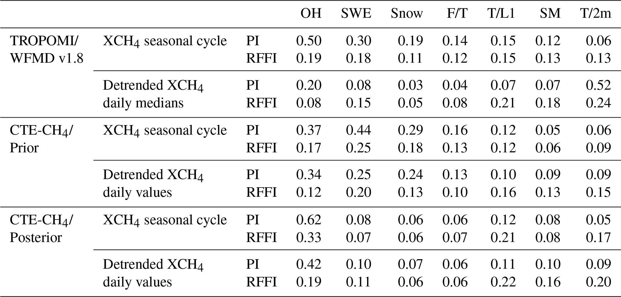
Table A2 Variable importance rankings based on permutation importance (PI) and random forest feature importance (RFFI) for TROPOMI/WFMD, CTE-CH₄/Prior, and CTE-CH₄/Posterior. Rankings are shown separately for the seasonal cycle and detrended daily values of XCH₄, for each environmental variable. A lower rank indicates higher importance (with 1 being the most important).

Appendix B: XCH₄ time series and fitted seasonal cycles

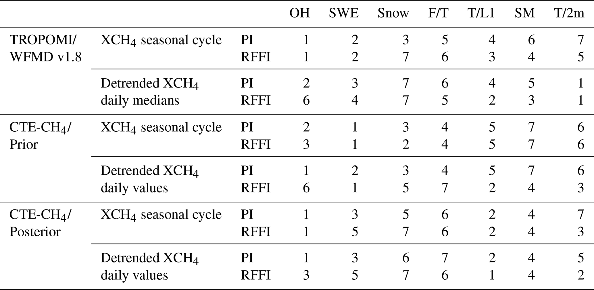
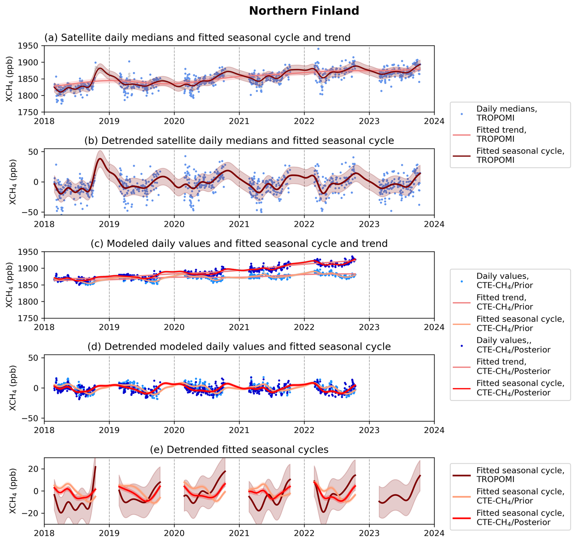
Figure B1 (a) TROPOMI WFMD daily median XCH₄ values (blue dots) with the fitted seasonal cycle and trend, including their uncertainties (red and shaded red), for Northern Finland. Panel (b) is the same as panel (a) but shows detrended TROPOMI WFMD XCH₄ time series. (c) CTE-CH₄ prior and posterior daily XCH₄ values (lighter- and darker-blue dots, respectively) and their fitted seasonal cycle and trend and uncertainties (lighter- and darker-red lines and corresponding shaded areas). Panel (d) is the same as panel (c) but shows detrended CTE-CH₄ time series. (e) Detrended fitted seasonal cycles and their uncertainties for TROPOMI WFMD and CTE-CH₄ prior and posterior XCH₄.

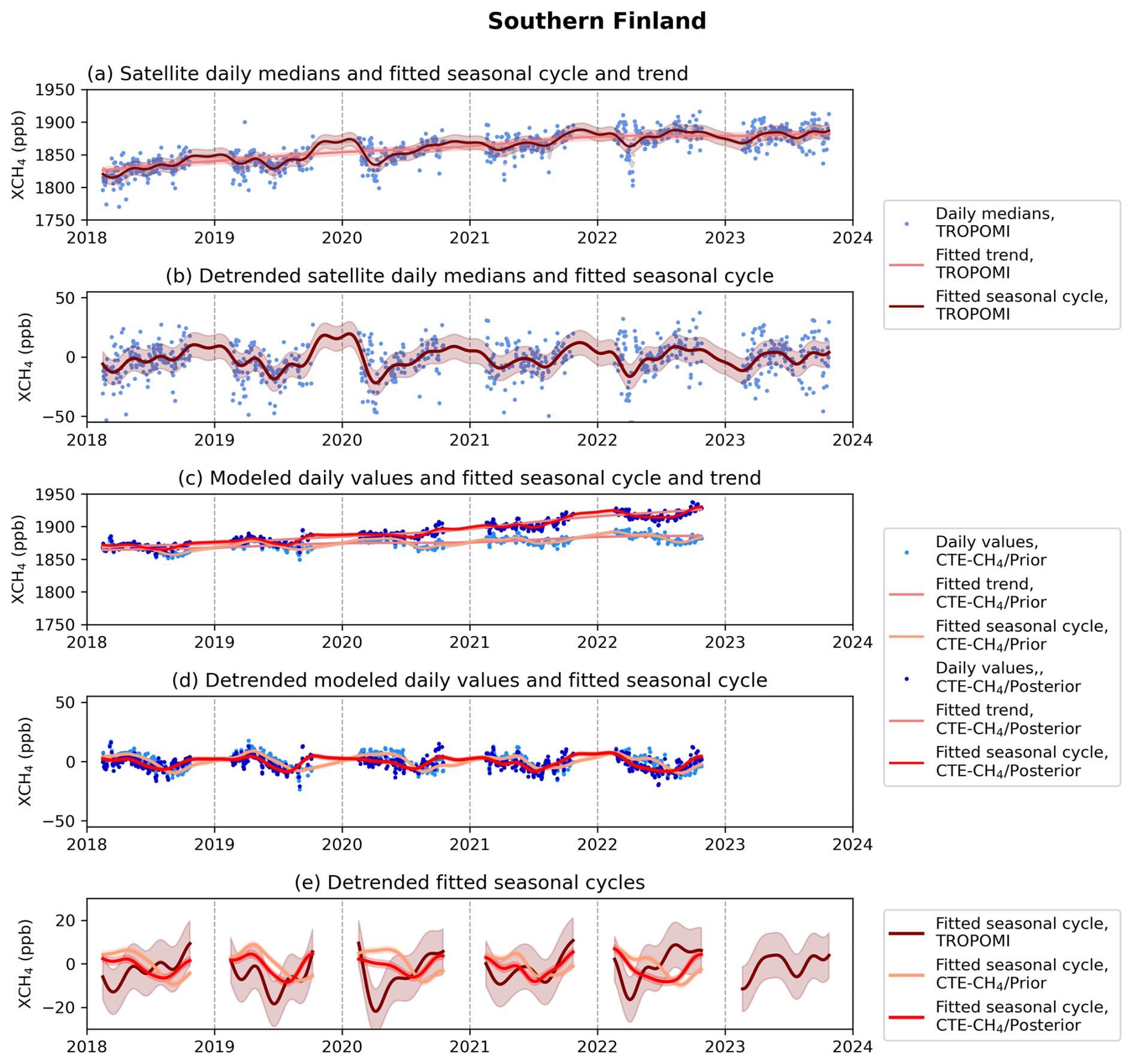
Figure B2 (a) TROPOMI WFMD daily median XCH₄ values (blue dots) with the fitted seasonal cycle and trend, including their uncertainties (red and shaded red), for Southern Finland. Panel (b) is the same as panel (a) but shows detrended TROPOMI WFMD XCH₄ time series. (c) CTE-CH₄ prior and posterior daily XCH₄ values (lighter- and darker-blue dots, respectively) and their fitted seasonal cycle and trend and uncertainties (lighter- and darker-red lines and corresponding shaded areas). Panel (d) is the same as panel (c) but shows detrended CTE-CH₄ time series. (e) Detrended fitted seasonal cycles and their uncertainties for TROPOMI WFMD and CTE-CH₄ prior and posterior XCH₄.

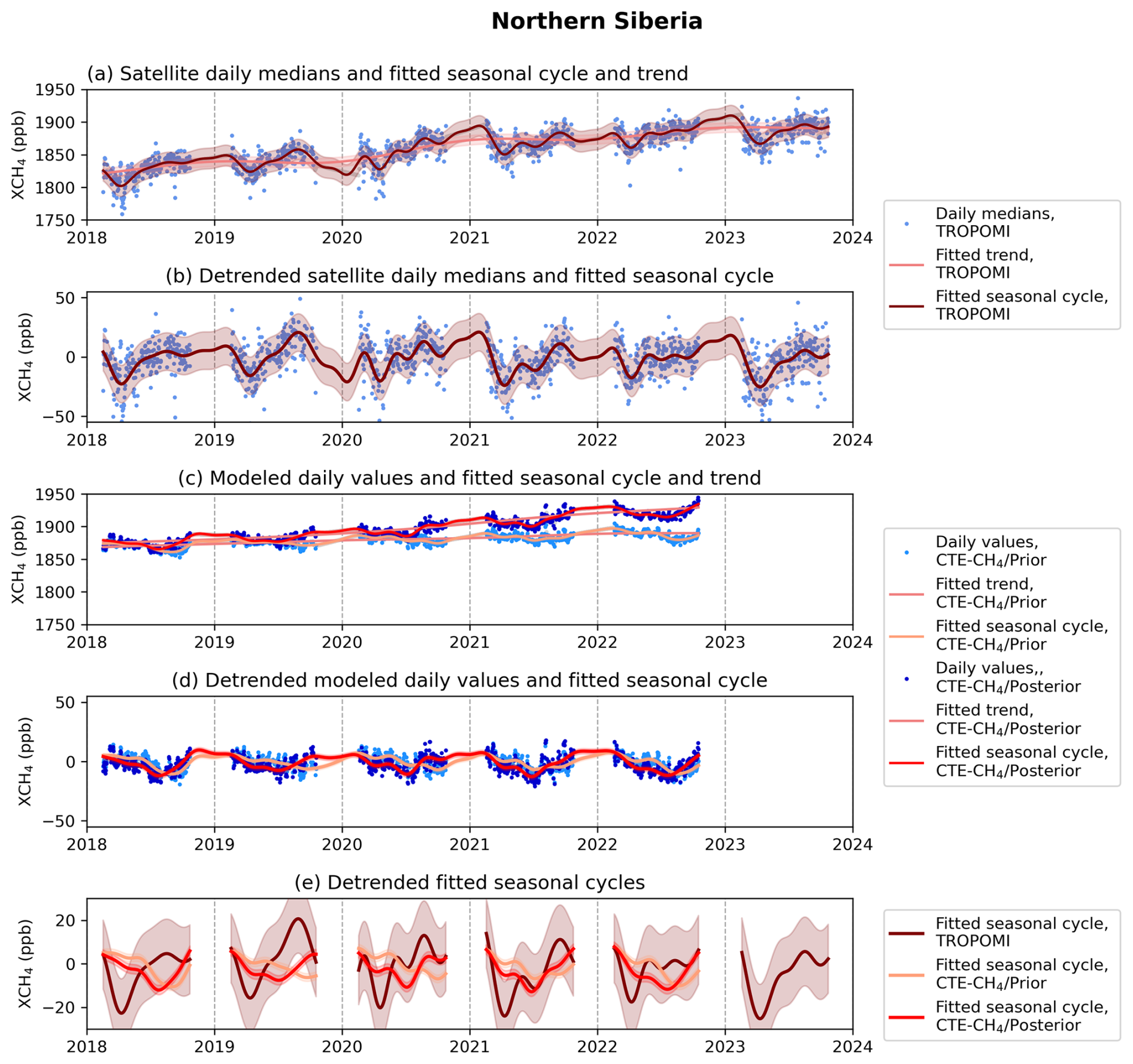
Figure B3 (a) TROPOMI WFMD daily median XCH₄ values (blue dots) with the fitted seasonal cycle and trend, including their uncertainties (red and shaded red), for Northern Siberia. Panel (b) is the same as panel (a) but shows detrended TROPOMI WFMD XCH₄ time series. (c) CTE-CH₄ prior and posterior daily XCH₄ values (lighter- and darker-blue dots, respectively) and their fitted seasonal cycle and trend and uncertainties (lighter- and darker-red lines and corresponding shaded areas). Panel (d) is the same as panel (c) but shows detrended CTE-CH₄ time series. (e) Detrended fitted seasonal cycles and their uncertainties for TROPOMI WFMD and CTE-CH₄ prior and posterior XCH₄.

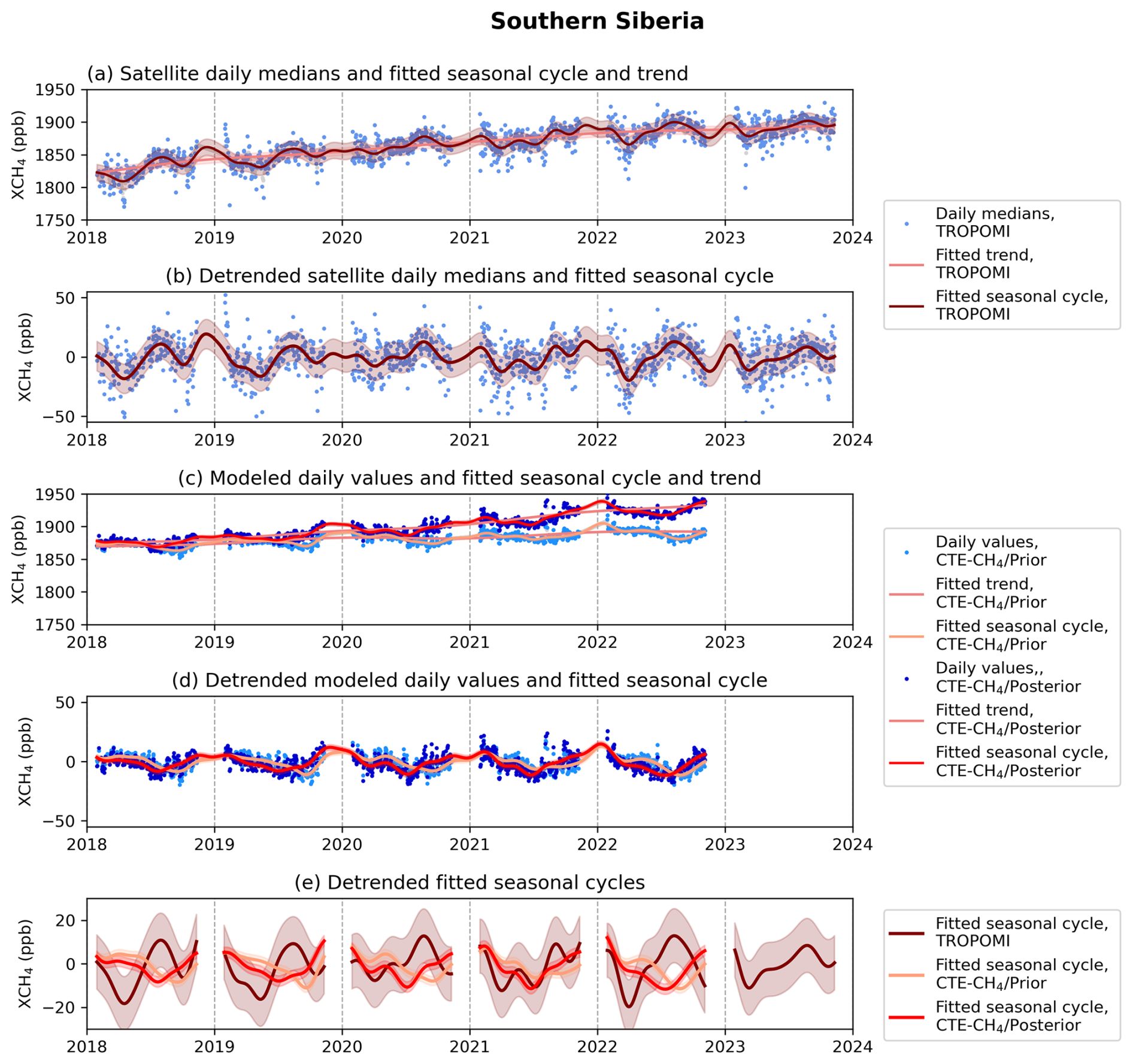
Figure B4 (a) TROPOMI WFMD daily median XCH₄ values (blue dots) with the fitted seasonal cycle and trend, including their uncertainties (red and shaded red), for Southern Siberia. Panel (b) is the same as panel (a) but shows detrended TROPOMI WFMD XCH₄ time series. (c) CTE-CH₄ prior and posterior daily XCH₄ values (lighter- and darker-blue dots, respectively) and their fitted seasonal cycle and trend and uncertainties (lighter- and darker-red lines and corresponding shaded areas). Panel (d) is the same as panel (c) but shows detrended CTE-CH₄ time series. (e) Detrended fitted seasonal cycles and their uncertainties for TROPOMI WFMD and CTE-CH₄ prior and posterior XCH₄.

Appendix C: Environmental time series

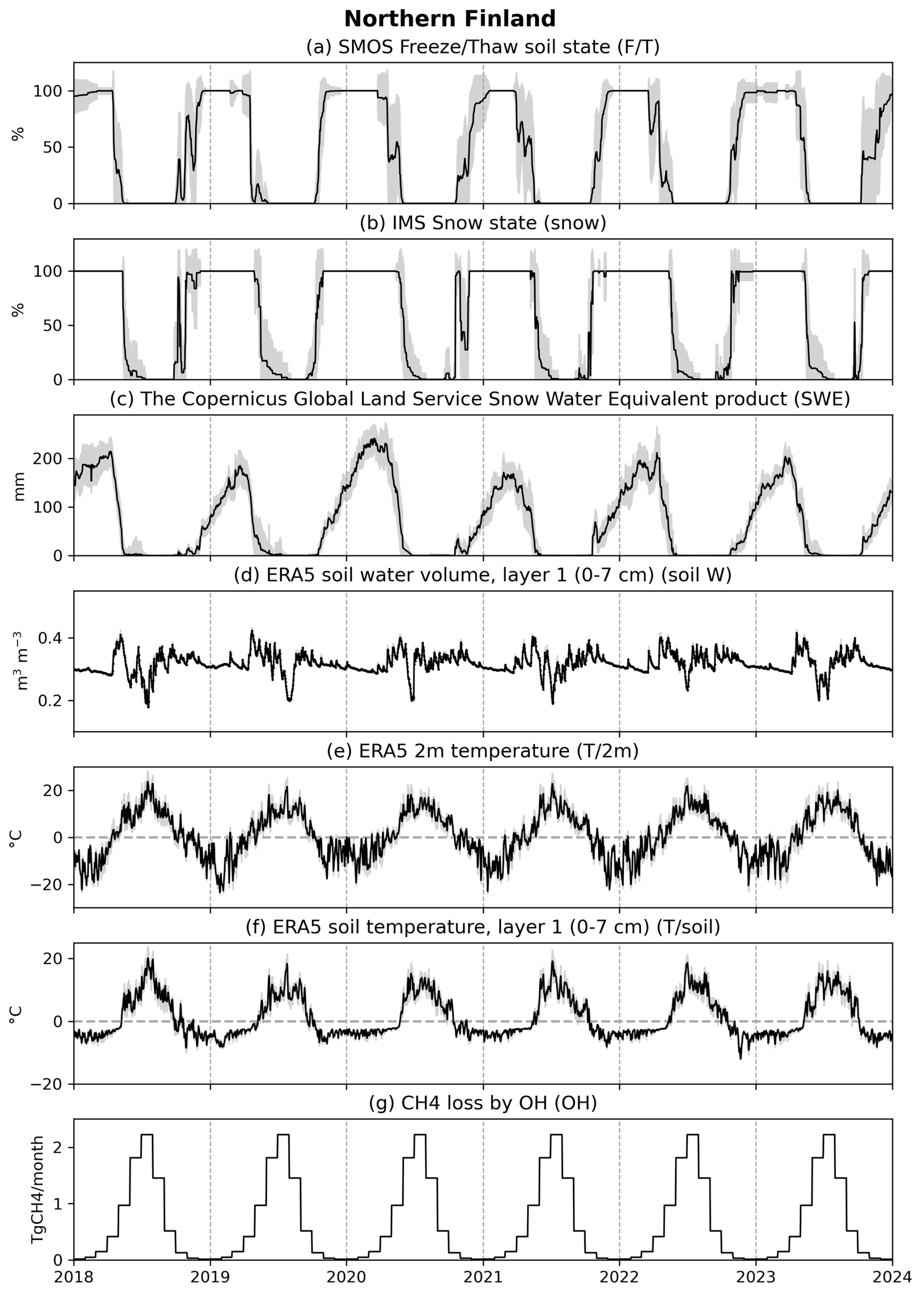
Figure C1 The black line shows the daily mean and the filled grey area shows the standard deviation of the (a) soil freeze–thaw state, (b) snow cover state, (c) snow water equivalent, (d) layer-1 soil water volume, (e) 2 m air temperature, (f) layer-1 soil temperature, and (g) CH₄ loss by OH for Northern Finland.

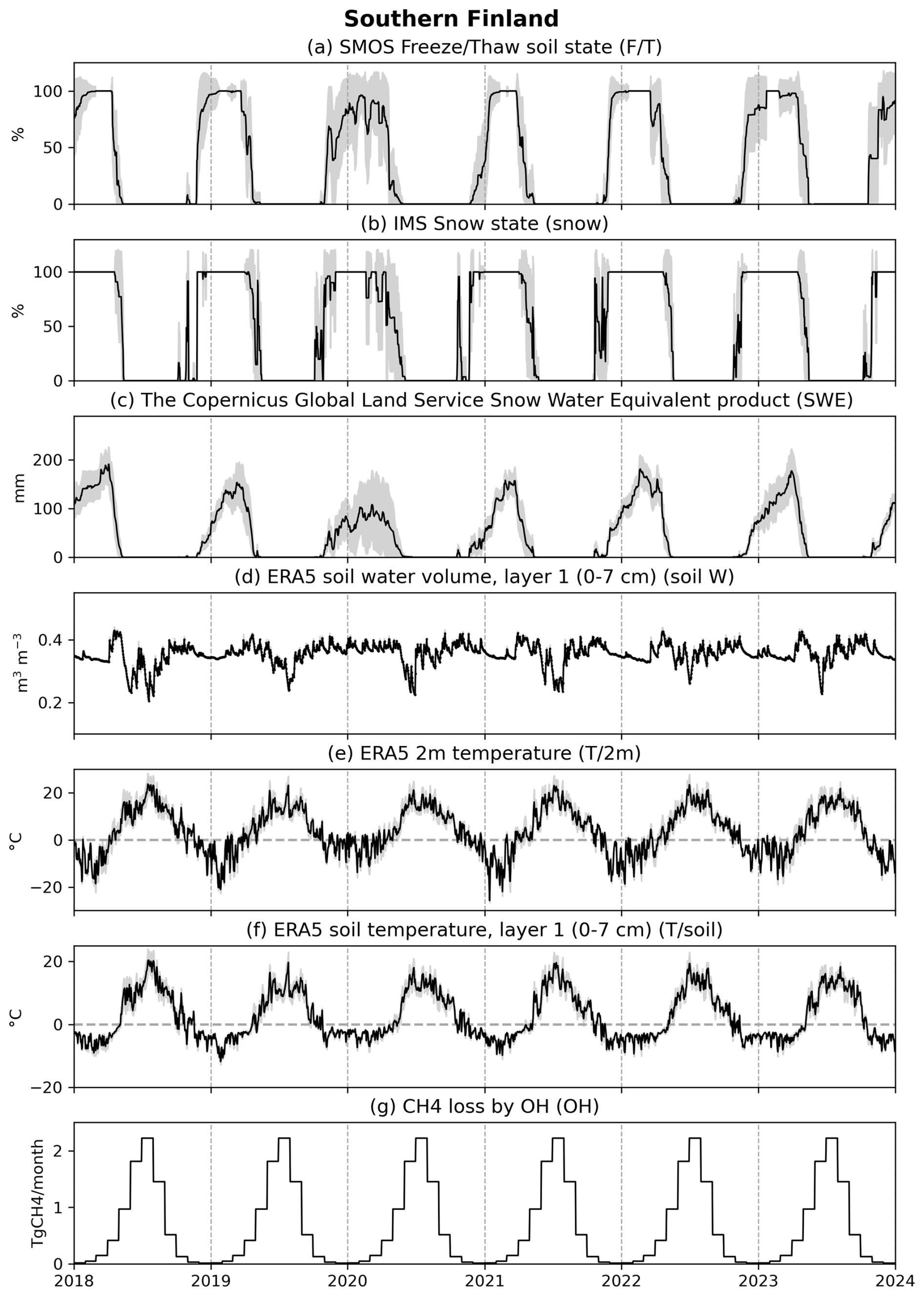
Figure C2 The black line shows the daily mean and the filled grey area shows the standard deviation of the (a) soil freeze–thaw state, (b) snow cover state, (c) snow water equivalent, (d) layer-1 soil water volume, (e) 2 m air temperature, (f) layer-1 soil temperature, and (g) CH₄ loss by OH for Southern Finland.

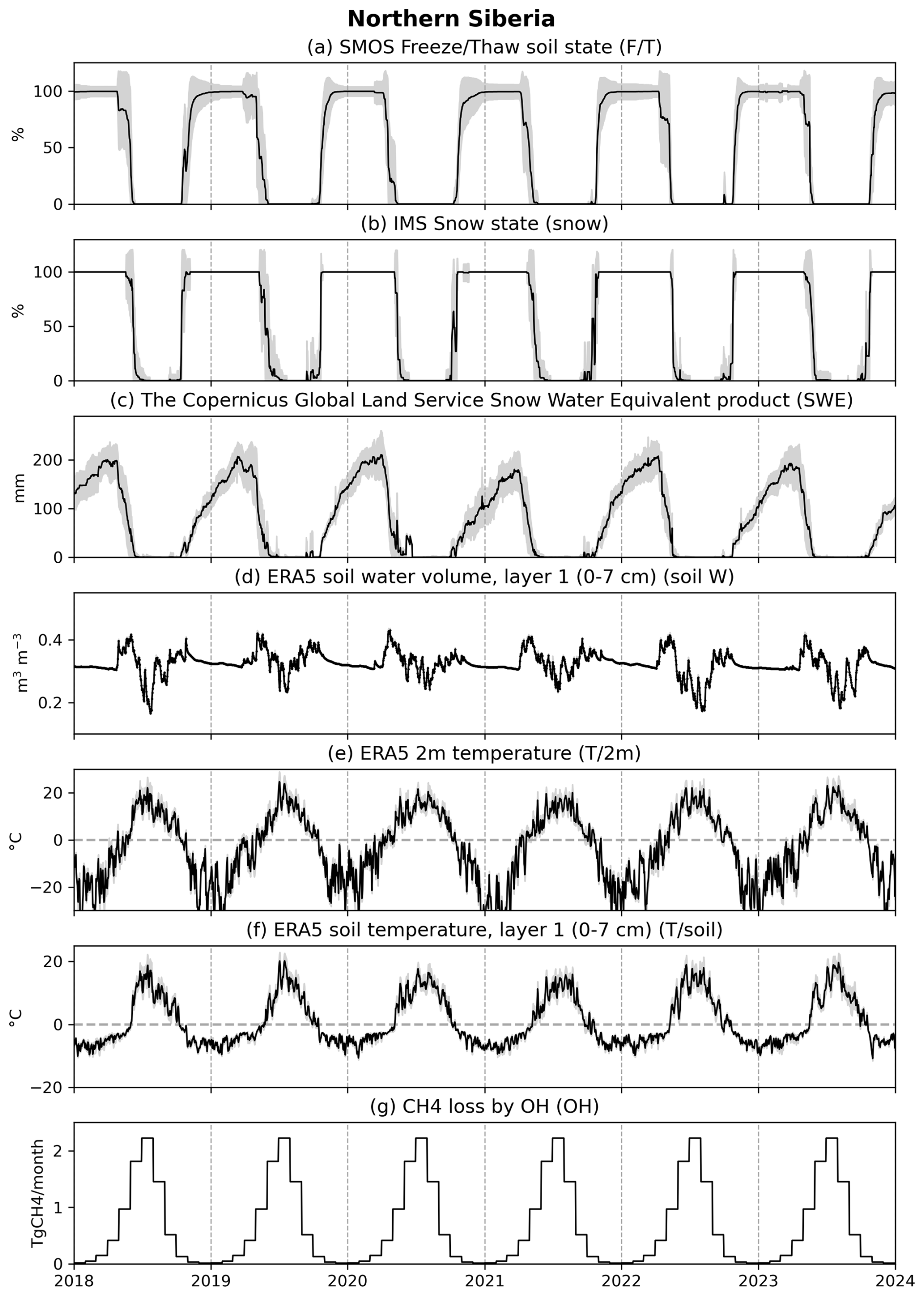
Figure C3 The black line shows the daily mean and the filled grey area shows the standard deviation of the (a) soil freeze–thaw state, (b) snow cover state, (c) snow water equivalent, (d) layer-1 soil water volume, (e) 2 m air temperature, (f) layer-1 soil temperature, and (g) CH₄ loss by OH for Northern Siberia.

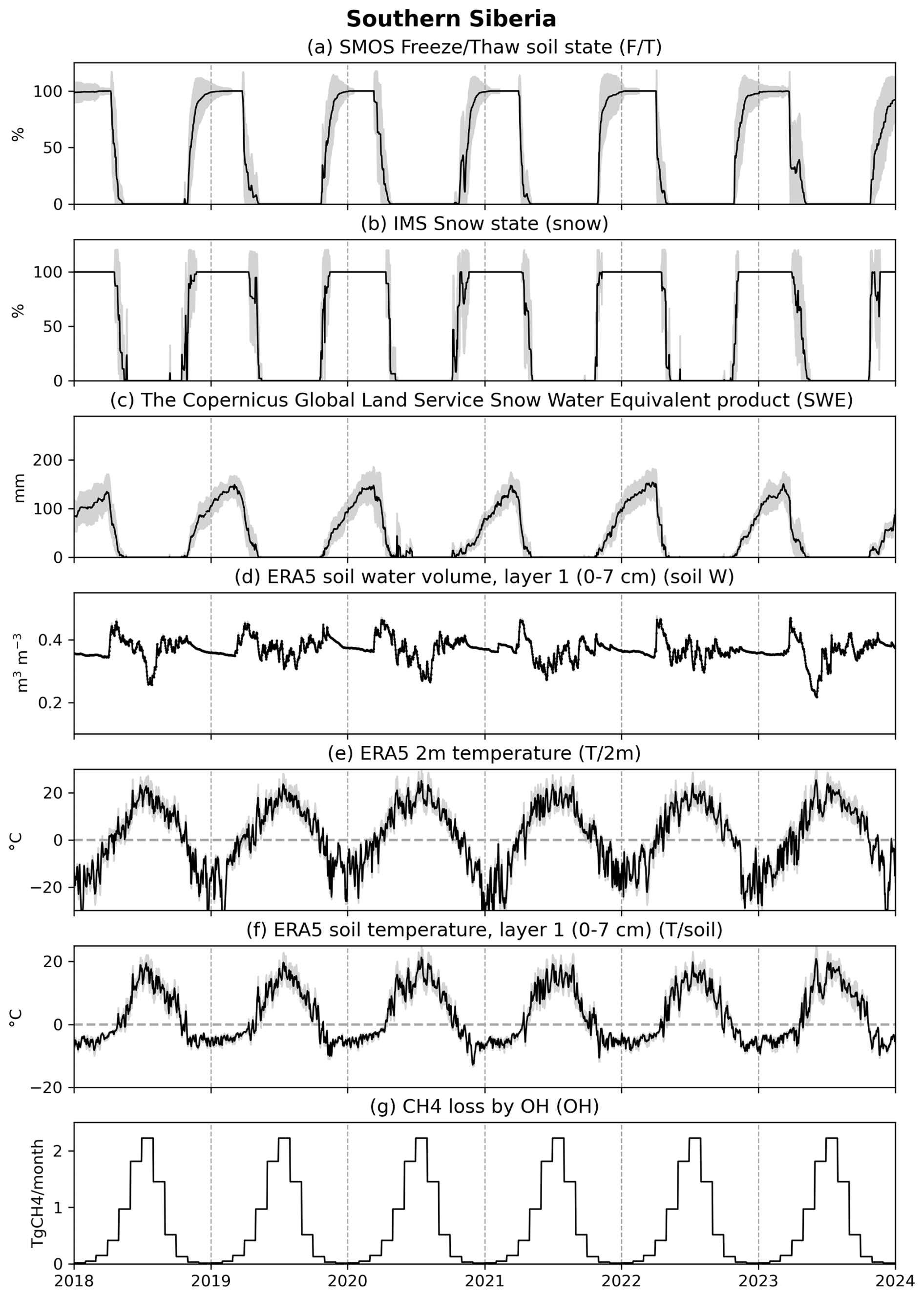
Figure C4 The black line shows the daily mean and the filled grey area shows the standard deviation of the (a) soil freeze–thaw state, (b) snow cover state, (c) snow water equivalent, (d) layer-1 soil water volume, (e) 2 m air temperature, (f) layer-1 soil temperature, and (g) CH₄ loss by OH for Southern Siberia.

Appendix D: Day-of-year time series

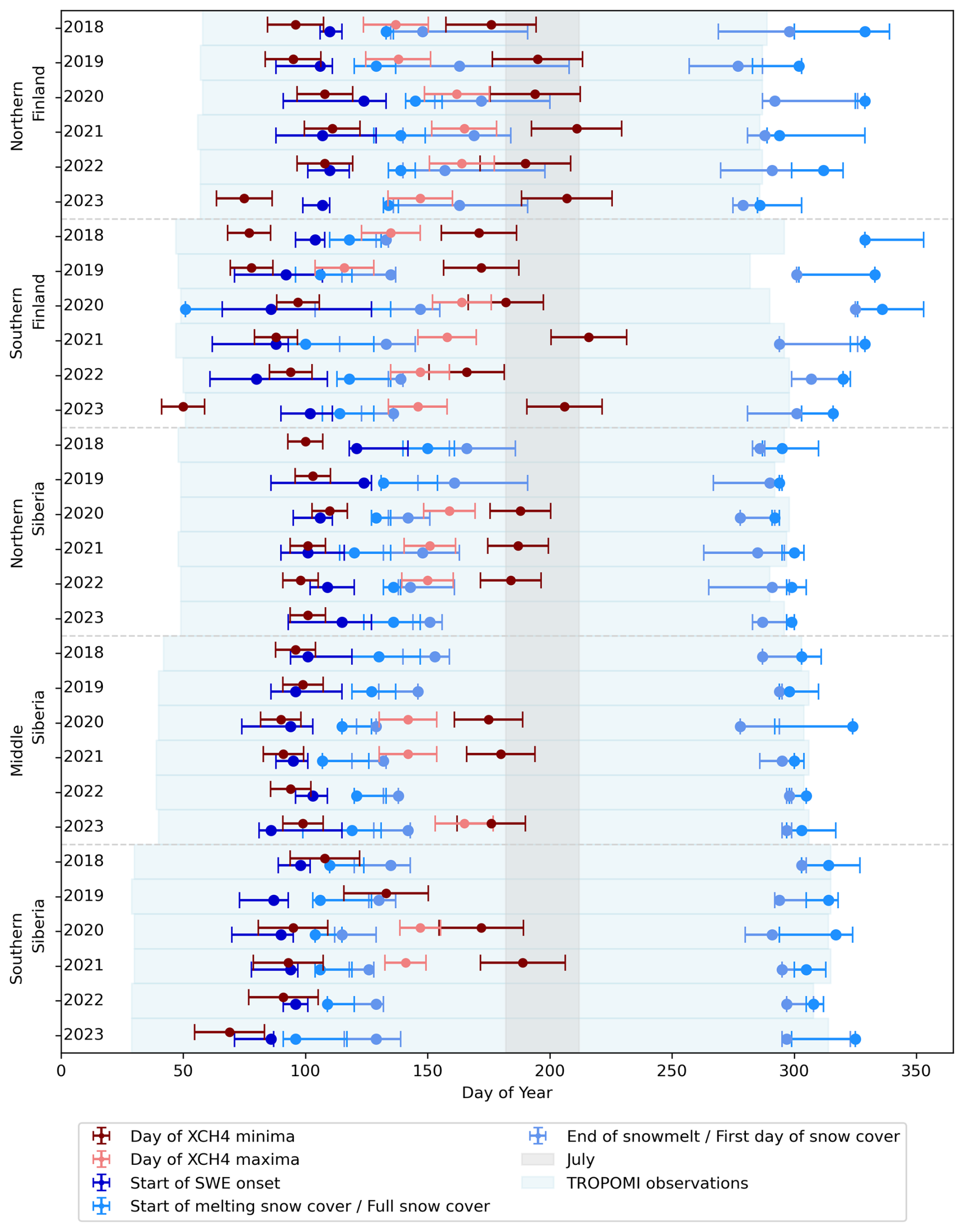
Figure D1 Timing of seasonal events related to snow cover and XCH₄ minima and maxima for different case study areas and years. The markers indicate the day of year of the XCH₄ seasonal cycle minima (dark-red circles), seasonal cycle maxima (light-red circles), start of SWE onset (dark-blue circles), beginning of snowmelt or onset of full snow cover (first day when snow cover fraction falls below or exceeds 0.9; medium-blue circles), and the end of snowmelt or start of the new snow season (first day when snow cover fraction falls below or exceeds 0.1; light-blue circles). Horizontal bars denote the uncertainty in the timing, and each region–year pair is plotted as a horizontal row. The shaded grey area marks the month of July, when CH₄ loss due to OH is at its maximum, and the blue background shading indicates the TROPOMI/WFMD observation period for each year.