Early Permian longitudinal position of the South China Block from brachiopod paleobiogeography

Knowledge of the past location of tectonic plates is essential to understanding the evolution of climate, ocean systems, and mantle flow. Tectonic reconstructions become increasingly uncertain as one moves further back in geological time. Paleomagnetic data constrain the past latitude of continental blocks but not their past longitude. For example, the longitude of the South China Block during Early Permian times is unknown. Paleobiogeographic data, which have long been used in tectonic reconstructions, make it possible to evaluate the faunal similarity between continental blocks. In this study, we use the global brachiopod distribution for two Early Permian time periods (Asselian–Sakmarian times between ∼ 298.9 and ∼ 290.1 Ma and Artinskian–Kungurian times between ∼ 290.1 and ∼ 274.4 Ma) from the Paleobiology Database to evaluate the correlation between faunal similarity and physical distance of continental blocks for three distinct tectonic reconstruction models. We use this approach to assess which of the three tectonic scenarios places the South China Block in a location that best accounts for the Early Permian brachiopod distribution data. Based on this analysis, the preferred tectonic reconstruction places the South China Block in a central position within the Paleo-Tethys Ocean instead of on its outskirts. The framework developed in this study is openly available and our approach can be applied to other tectonic blocks, time periods, and faunal data.

1 Introduction

Plate tectonic motions strongly influence Earth's internal and external systems (Valentine and Moores, 1970; Müller et al., 2008; Flament et al., 2017; Dutkiewicz et al., 2024), making it important to develop robust models of plate tectonic configurations to understand how these systems have evolved over geological time. Constraining the latitude of a tectonic plate over time can be achieved directly via paleomagnetic analysis (Torsvik and Van der Voo, 2002; Krivolutskaya et al., 2016), which determines the distance from the North Pole or South Pole. Paleolongitude, however, cannot be constrained in absolute terms and must instead be determined in relation to other features. This is commonly done by using either geophysical data from the oceanic lithosphere (Scotese, 2004; Seton et al., 2012), which are limited back in time due to subduction of the oceanic lithosphere, or by relating orogens and stratigraphy across plate boundaries (Lehmann et al., 2010), which cannot provide information about isolated tectonic plates.

One method to constrain the relative locations of isolated tectonic blocks and for reconstructions at older times is paleobiogeographic similarity, which compares the similarity of ancient faunal assemblages between regions as a function of physical distance between tectonic blocks. Fossil data can be used to evaluate the past distance between tectonic plates (e.g. Piccoli et al., 1991; Lees et al., 2002) by assuming that the similarity between the faunal assemblages of two plates decreases as the physical distance between the plates increases. This assumption is based on the principle that continental configuration influences faunal distribution (Shi, 2001a, b; Zaffos et al., 2017). The configuration of tectonic plates controls climate (Valentine and Moores, 1972), ocean circulation (Valentine, 1971; Allison and Wells, 2006), and the locations of land and ocean barriers (Valentine and Moores, 1970), which are all factors that affect faunal distribution. Indeed, faunal similarity is expected to be negatively correlated with distance (Valentine, 1966), because the spread of species to geographically close areas is easier than to geographically distant areas. Statistical measures of the similarity between two faunal assemblages consider binary presence–absence data to assess either overlapping or unique fauna between two regions (Shi, 1993). Here, we present a new framework to apply these quantitative measures globally through a case study of the South China Block during the Early Permian.

The South China Block (SCB) was isolated within large ocean basins throughout Early Permian times (between ∼ 298.9 and ∼ 274.4 Ma; Cohen et al., 2024), which causes a lack of geological evidence linking it to other blocks, thus limiting the available data to constrain the longitudinal position of the plate. In this contribution, we consider the Early Permian location of the SCB for three different plate tectonic reconstructions, with two placing it on the boundary of the Panthalassan Ocean and Paleo-Tethys Ocean (Wright et al., 2013; Matthews et al., 2016) and the other placing it much further west, centrally within the Paleo-Tethys Ocean (Young et al., 2019). Paleomagnetic analysis of the Emeishan large igneous province (Emeishan LIP) during mid-Permian times constrains the paleolatitude of the SCB to low latitudes around the Equator (Krivolutskaya et al., 2016) at ∼ 260 Ma (Zhong et al., 2014). While this is not a direct latitudinal placement of the SCB during Early Permian times, it does provide a known latitude immediately following Early Permian times; consequently, the SCB can be assumed to have been near this latitude during Early Permian times.

The differences in the proposed position of the SCB among the three reconstructions are largely due to differing methods to infer its Early Permian longitude. The eruption of the Emeishan LIP is attributed to a deep mantle plume, which has been suggested to originate from the edges of the African and Pacific large low-shear-velocity provinces (LLSVPs) (Torsvik et al., 2008). The link between mantle plumes and LLSVPs has been used in some reconstructions to infer the longitude of plates on which LIPs are preserved, by placing such plates at the margin of one of the LLSVPs with the assumption that the LLSVPs have remained stationary since the Early Permian (Torsvik et al., 2010). In contrast, in some other reconstructions (e.g. Scotese, 2004), the longitude is based on interpretations of tectonic activity preserved in the rock record. These methods to determine paleolongitudes introduce uncertainties into the tectonic reconstructions; however, this is unavoidable because no direct evidence exists to constrain the past longitudinal position of plates. By using the same faunal dataset to test each of the three tectonic reconstructions, the relationship between faunal similarity and physical distance is only influenced by the plate configurations for each tectonic reconstruction. This makes it possible to use statistical measures of faunal similarity to assess the compatibility of each of these SCB paleolongitude scenarios with a global plate tectonic configuration, providing a test of paleolocation independent of the assumptions used to reconstruct the SCB and the uncertainties inherent to them.

2 Data

2.1 Plate tectonic reconstructions

We consider three tectonic reconstructions that are based on different approaches and present large variations in the location of the SCB during Early Permian times: Wright et al. (2013), Matthews et al. (2016), and Young et al. (2019), labelled here as Y19, M16, and W13, respectively. Reconstruction W13 was built upon previous plate models from Scotese (2004), Golonka (2007), and Seton et al. (2012) by developing an updated location for the Australian plate based on paleoenvironments interpreted from faunal data. The placement of the SCB was an estimated transitional position based on information of tectonic activity in the rock record (Scotese, 2004). For reconstruction M16, the SCB was placed further east (133° E at 277 Ma) based on work by Domeier and Torsvik (2014) which attributes the Emeishan LIP to the western margin of the Pacific LLSVP under the assumption that the LLSVP has remained spatially fixed since the Emeishan LIP emplacement (Conrad et al., 2013). Reconstruction Y19 was built based on reconstruction M16 using the same set of tectonic plate geometries, which makes a direct comparison between these two reconstructions possible. The global plate velocities required by the plate tectonic configuration used for reconstruction M16 during the Permian are large, requiring the SCB to move at speeds of up to 40 cm yr⁻¹ between 260 and 250 Ma, which is tectonically unreasonable (Zahirovic et al., 2015; Young et al., 2019). Reconstruction Y19 was designed to have global plate configurations that give more tectonically reasonable plate velocities. This was done for the placement of the SCB by considering both records of tectonic activity to constrain the SCB longitude to a transitional position (similar to the approach used for reconstruction W13) which happens to coincide with the edge of a mobile large basal mantle structure produced by a mantle flow model (Young et al., 2019). While the edges of plume-generating structures were considered for the placement of the SCB during the development of both reconstructions Y19 and M16, there remains key differences between the two. For reconstruction Y19, the SCB was placed over the eastern margin of the African basal mantle structure predicted by a mantle flow model, whereas the SCB was tied to the seismically imaged western margin of the Pacific LLSVP for reconstruction M16. Paleomagnetic data were used as the latitudinal constraint for the development of all three reconstructions, which is particularly effective because the north–south uncertainty that is typically a concern for paleomagnetic data is less pronounced for these SCB positions as it was situated near the Equator. Here, we investigate the compatibility of these different plate tectonic reconstruction models with faunal data, including reconstructions M16 and Y19 that are designed using competing ideas on the mobility of LLSVPs.

We used 277 Ma as the representative age of the Early Permian to perform the analysis because all three plate tectonic reconstructions have an explicitly defined position for the SCB at that age. This is particularly important for reconstruction W13, as positions for earlier Permian times are interpolated between the position at 277 Ma and the next explicitly defined position during Late Carboniferous times at 306 Ma. Furthermore, profound climatic change occurred during Early Permian times (Fielding et al., 2008), with the peak of the late-Paleozoic icehouse occurring near the Asselian–Sakmarian boundary (Fielding et al., 2008; Scotese et al., 2021), followed by the Artinskian Warming Event (Marchetti et al., 2022) which raised global average temperatures by 3–4 °C (Scotese et al., 2021). This led to major changes in brachiopod faunal assemblages (Shen et al., 2013). Because of these climatic shifts and of the long duration of Early Permian times (27 Myr), over which tectonic plates may have moved considerably, we divided Early Permian times into two intervals: Asselian–Sakmarian times (between ∼ 298.9 and ∼ 290.1 Ma; reconstructed at 295 Ma) and Artinskian–Kungurian times (between ∼ 290.1 and ∼ 274.4 Ma; reconstructed at 277 Ma). We focused on Artinskian–Kungurian times because there are more fossil occurrences and all three tectonic reconstructions have an explicitly defined position at 277 Ma. Data were also analysed for Asselian–Sakmarian times to investigate the sensitivity of results to selected data and to showcase the applicability of our method to distinct periods. At 277 Ma, the SCB was placed further west in reconstruction Y19 by approximately 3300 km compared to reconstruction M16 and 2500 km compared to reconstruction W13; the centroid of the SCB was located at longitude 103° E in reconstruction Y19, 133° E in reconstruction M16, and 125° E in reconstruction W13. Because these reconstructed locations are different, we anticipate that their respective compatibility with the brachiopod distribution can be established quantitatively.

2.2 Brachiopod fossil data from the Paleobiology Database

The distribution of Early Permian brachiopods can be summarized into three realms with distinct brachiopod faunal assemblages (Waterhouse and Bonham-Carter, 1975): Boreal (northern latitudes), Paleoequatorial, and Gondwanan (southern latitudes). These realms exhibit biogeographic patterns that match those expected from their continental configuration. The Gondwanan and Boreal realms are dominated by large continental landmasses and cold-water environments that produce low diversity, while the Paleoequatorial realm, characterized by warmer waters and many small island regions, presents a high degree of biodiversity (Shen et al., 2013). The consistency between expected biogeographic patterns based on continental configuration and the biogeographic realms suggests that the Early Permian brachiopod distribution should match the expected negative trend of decreasing faunal similarity with distance, making them an appropriate dataset for this study. Brachiopod fossils are also commonly used for understanding Palaeozoic biogeographic patterns, as they were the most dominant Palaeozoic benthic components under most marine conditions.

In order to conduct a reliable biogeographic approach at a global scale, brachiopod biogeographic data were selected at the genus level; species-level data are also available, but genus-level data are generally less affected by taxonomic biases. The biogeographic data were obtained from the Paleobiology Database, which provided an open, solid, and updated dataset solely based on published taxonomies. The validity of the genera included in the dataset was checked before performing the biogeographic analyses, and reports of genera with uncertain identification were excluded. To further alleviate taxonomic uncertainty and demonstrate the flexibility of the developed framework, a sensitivity analysis was performed at the family level, with results presented for the strongest subset of results.

Early Permian brachiopod biogeographic data were downloaded from the Paleobiology Database (Paleobiology Database, 2025) on 11 July 2025 for both the Artinskian–Kungurian interval and Asselian–Sakmarian interval. Data on “occurrences” were retrieved for the taxa “brachiopoda” with a taxonomic resolution of “lump by genus”, excluding uncertain genera and using the following parameters: the “interval or Ma range” was set equal to 290.1–274.4 for Artinskian–Kungurian times and to 298.9–290.1 for Asselian–Sakmarian times, the “age rule” was set to “contains”, “outputs” were set to “coordinates”, and “time binning” and “classification” were enabled. The paleobiogeographic dataset consisted of 9988 fossil occurrences made up of 502 unique genera belonging to 81 families for Artinskian–Kungurian times and of 4670 fossil occurrences made up of 359 unique genera belonging to 73 families for the Asselian–Sakmarian times. We analysed the following data frame columns: “genus” (genus name), “lat” (latitude), “lng” (longitude), and “family” (family name).

3 Methods

3.1 Biogeographic indices

Several binary similarity indices have been independently developed (Jaccard, 1907; Simpson, 1960; Lees et al., 2002) using varying conceptual bases to measure the similarity between two faunal datasets (Hohn, 2018). These indices are useful tools in paleobiogeography to quantify faunal similarity between biogeographic regions by comparing regional biota datasets based on presence–absence data (Fallaw and Dromgoole, 1980; Shi, 1993; Schmachtenberg, 2008). The underlying conceptual basis for each index introduces unique statistical biases for each measure, so multiple faunal similarity indices are commonly used in conjunction (Simpson, 1960; Schmachtenberg, 2008; Hohn, 2018).

The Jaccard index (JC;  Jaccard, 1907) measures the true similarity between any two sets of fauna, assuming that any differences in biodiversity are real. This means that the sampled distribution is assumed to be an accurate representation of the true distribution. It is calculated by dividing the intersection of the biota sets by the union of the biota sets:

$$\begin{array}{}\text{(1)}& \text{JC}={\displaystyle \frac{S_{\mathrm{1}}\cap S_{\mathrm{2}}}{S_{\mathrm{1}}\cup S_{\mathrm{2}}}},\end{array}$$

where S₁ is the taxa set for the less diverse region (less genera) and S₂ is the taxa set for the more diverse region (more genera).

The Simpson index (SC;  Simpson, 1960) takes into account that some differences in biodiversity between regions could be a result of sampling bias. This is done by not including the number of genera in the more diverse region in the calculation:

$$\begin{array}{}\text{(2)}& \text{SC}={\displaystyle \frac{S_{\mathrm{1}}\cap S_{\mathrm{2}}}{n\mathrm{1}}},\end{array}$$

where n₁ is total number of genera in the less diverse region S₁.

The two-plate mean endemism index (ME;  Lees et al., 2002) accounts for differences in area and biogeographic effects between two regions by averaging the proportions of endemic fauna in each region:

$$\begin{array}{}\text{(3)}& \text{ME}={\displaystyle \frac{\left(\frac{S_{\mathrm{1}}-S_{\mathrm{2}}}{n_{\mathrm{1}}}\right)+\left(\frac{S_{\mathrm{2}}-S_{\mathrm{1}}}{n_{\mathrm{2}}}\right)}{\mathrm{2}}},\end{array}$$

where n₂ is the number of genera in the more diverse region S₂. JC and SC measure faunal similarity and are expected to be negatively correlated with distance, while ME measures faunal difference and is expected to be positively correlated with distance. For consistency, we used $\text{cME}=\mathrm{1}-\text{ME}$, which is expected to be negatively correlated with distance. Values for each of the three indexes JC, SC, and cME range between 0, indicating complete dissimilarity, and 1, indicating complete similarity.

To calculate Early Permian faunal similarity indexes, the present-day fossil locations were first transformed to their Early Permian paleolocations. The present-day latitude and longitude of each fossil occurrence were used to define a point on the Earth, which was then converted to a feature collection saved in a GPlates Markup Language (“.gpml”) file (Müller et al., 2018) using PyGPlates (Mather et al., 2024). A “point-in-polygon” test was carried out with PyGPlates to (1) assess which tectonic block each point belonged to and (2) attribute the corresponding plate ID specific to each tectonic reconstruction. This made it possible to split the data into subsets of biota for each plate and to reconstruct the points back in time using PyGPlates. As a result of the reconstruction to paleolocations, one fossil occurrence point was located on a W13 plate boundary, and two points for reconstructions M16 and Y19 were located within a plate void. These points were discarded, as they represented minor portions of the total dataset and including them would have introduced errors.

3.2 Calculating distance between plates

After each plate was assigned a faunal assemblage, we calculated physical distances between each plate to establish the relationship between faunal similarity and distance. The physical distance between plates was calculated as great-circle distances along the surface of a sphere with a constant radius of 6371 km between plate centroids using PyGPlates. Some plate IDs were assigned to multiple polygons that collectively represented a larger plate. In such cases, a new polygon was created from the multiple plate centroids, and the centroid of that new polygon was used as reference for that plate.

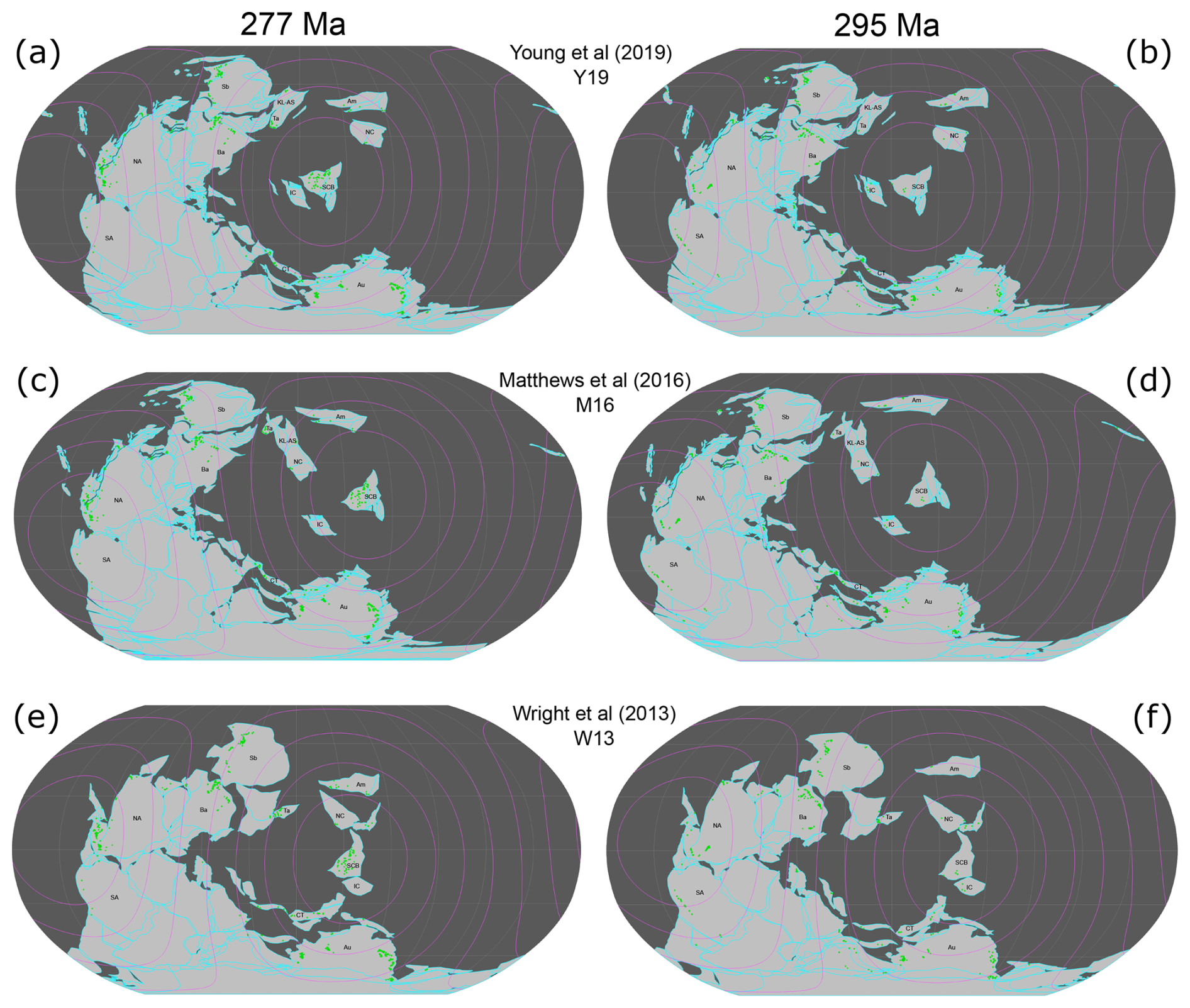
Figure 1 All three considered tectonic reconstructions at 295 and 277 Ma with distance ranges as concentric circles from 4000–16 000 km from the SCB in 2000 km increments. Fossil occurrences are shown as green circles, plate outlines as open cyan polygons, continents as filled light-grey polygons, and oceans in dark grey. The names of tectonic blocks are abbreviated as follows: Am: Amuria; Au: Australia; Ba: Baltica; CT: Cimmerian terranes; IC: Indochina; KL-AS: Kunlun–Ala Shan; NA: North America; NC: North China; SA: South America; Sb: Siberia; Ta: Tarim.

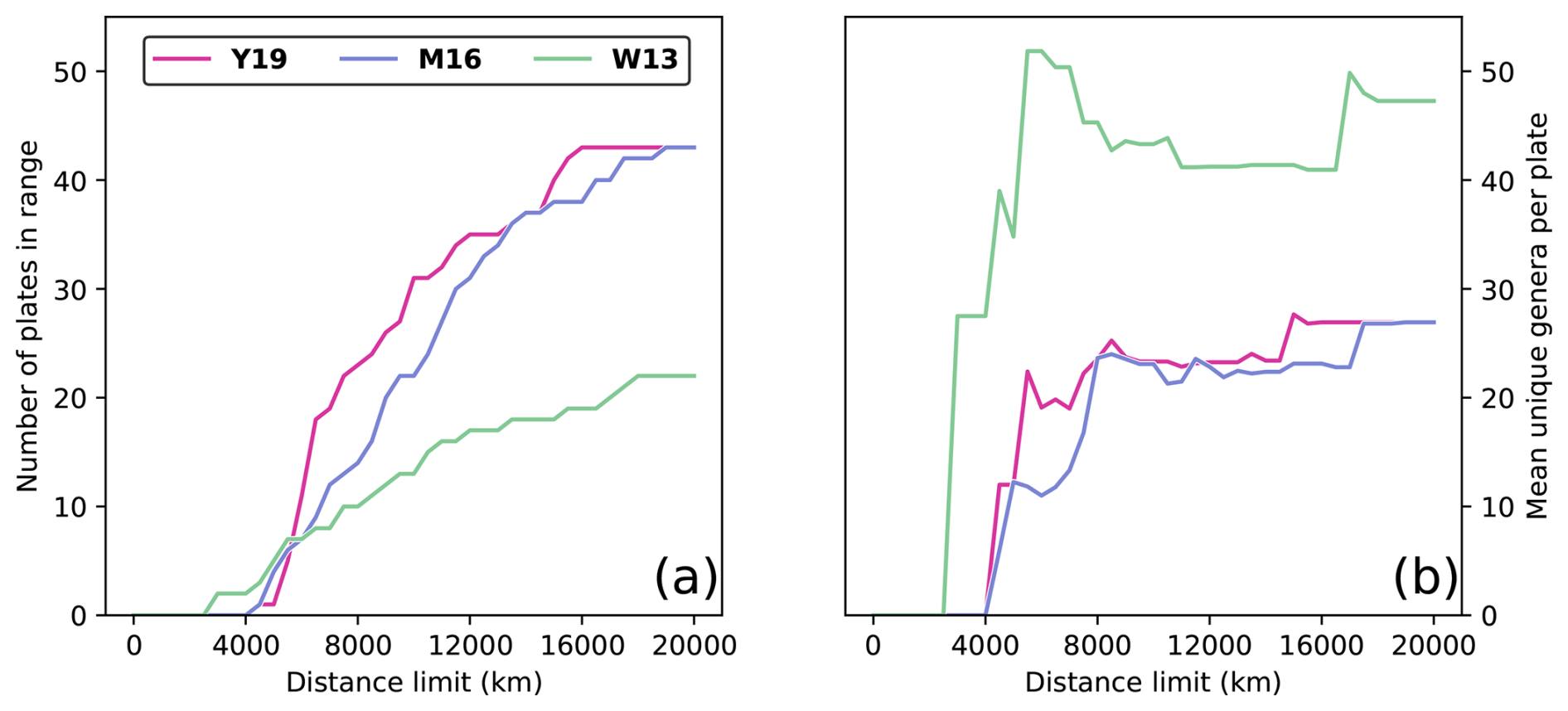
Figure 2 Evaluating the effect of the distance limit on sample sizes during Artinskian–Kungurian times, considering only plates with at least one fossil occurrence. (a) Number of plates that have centroids within the distance limit from the SCB centroid for each of the three considered tectonic reconstructions W13, M16, and Y19. (b) Average number of genera per plate for the set of plates within a given distance limit for each of the three considered tectonic reconstructions.

Distance limits d_l from the SCB were imposed to obtain meaningful results. The distance limit must include a large enough sample of plates to obtain a statistically meaningful relationship between distance and similarity (Fig. 2a) and to reduce the impact of noise from random sampling errors that are inherent to paleontological datasets. Larger distances, however, introduce continental land barriers between plates (Fig. 1), which complicates the relationship between biogeographic similarity and distance by considering great-circle arc distances that are longer than reasonably expected for brachiopod migratory distances, because brachiopods are marine organisms. It is also important that plates within a distance limit present, on average, a large enough faunal assemblage to make meaningful comparison with the SCB faunal assemblage (Fig. 2b). For each reconstruction, we considered distance limits beginning at the distance of the closest plate centroid, increasing by steps of 50 km in radius until a maximum radius of 20 100 km (just over half of Earth's maximum circumference) to test progressively larger tectonic plate datasets (see concentric circles in Fig. 1). A plate was considered within range if the minimum distance between the plate centroid and the centroid of the SCB was smaller than the distance limit. If a plate centroid was within range, all fossil occurrences on the plate were considered.

3.3 Statistical tests and data processing

All three biogeographic index values were calculated for each plate pair that consisted of the SCB and another plate. The Spearman rank correlation coefficient (r_s) was used to determine the monotonicity and direction of the relationship between faunal similarity as measured by the biogeographic indices and physical distance. A negative r_s is expected if faunal similarity decreases as physical distance increases. The Spearman correlation coefficient was selected, as it has been argued that faunal similarity should decrease exponentially with physical distance (Piccoli et al., 1991); however, it has been found that using a natural logarithm transformation on the faunal similarity data does not always provide better results (Schmachtenberg, 2008), and often these results are very similar. As the Spearman rank correlation tests only for monotonic relationships, it has equal power in determining a relationship, regardless of whether it is linear or exponential. The Spearman rank correlation is also more robust to outliers and tailed distributions than the linear Pearson correlation coefficient (De Winter et al., 2016), which helps mitigate the uncertainty inherent to working with fossil datasets. The final benefit of the Spearman correlation is that, as it is a rank correlation which tests only for monotonicity, the order in which plates are encountered with increasing distance is more important than the distances themselves, making this test a more robust measure of global plate tectonic configuration than a purely linear or logarithmic relationship.

We carried out a one-tailed test to determine the statistical significance of the relationship between faunal similarity and physical distance for each distance limit in each tectonic reconstruction. We formulated the null hypothesis that faunal distribution was random and unrelated to physical distance between plates, which was rejected at the 95 % confidence interval if the p value was less than 0.05. A one-tailed test was chosen because it allowed us to test for statistical significance only if the relationship was negative (decreasing faunal similarity as physical distance increases). We considered a positive global relationship (faunal similarity increases with physical distance) to be more indicative of an incorrect plate tectonic configuration rather than a true relationship. The strength of the correlation between faunal similarity and physical distance and the statistical significance of those relationships were then used to determine the most appropriate reconstruction and ideal distance limit within that reconstruction.

Data were prepared and analysed using Python Jupyter notebooks (Kluyver et al., 2016). The pandas (McKinney, 2010), SciPy (Virtanen et al., 2020), and NumPy (Harris et al., 2020) libraries were used for statistical methods; the PyGPlates (Müller et al., 2018; Mather et al., 2024) library was used for reconstruction and geospatial operations; and the Matplotlib library (Hunter, 2007) was employed to plot results.

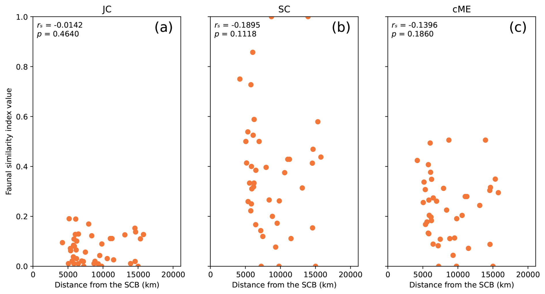
Figure 3 All considered biogeographic similarity indexes calculated between the SCB and all 43 other plates with genus-level brachiopod occurrences in reconstruction Y19 at 277 Ma, used to represent Artinskian–Kungurian times. The r_s and p values are presented for each index.

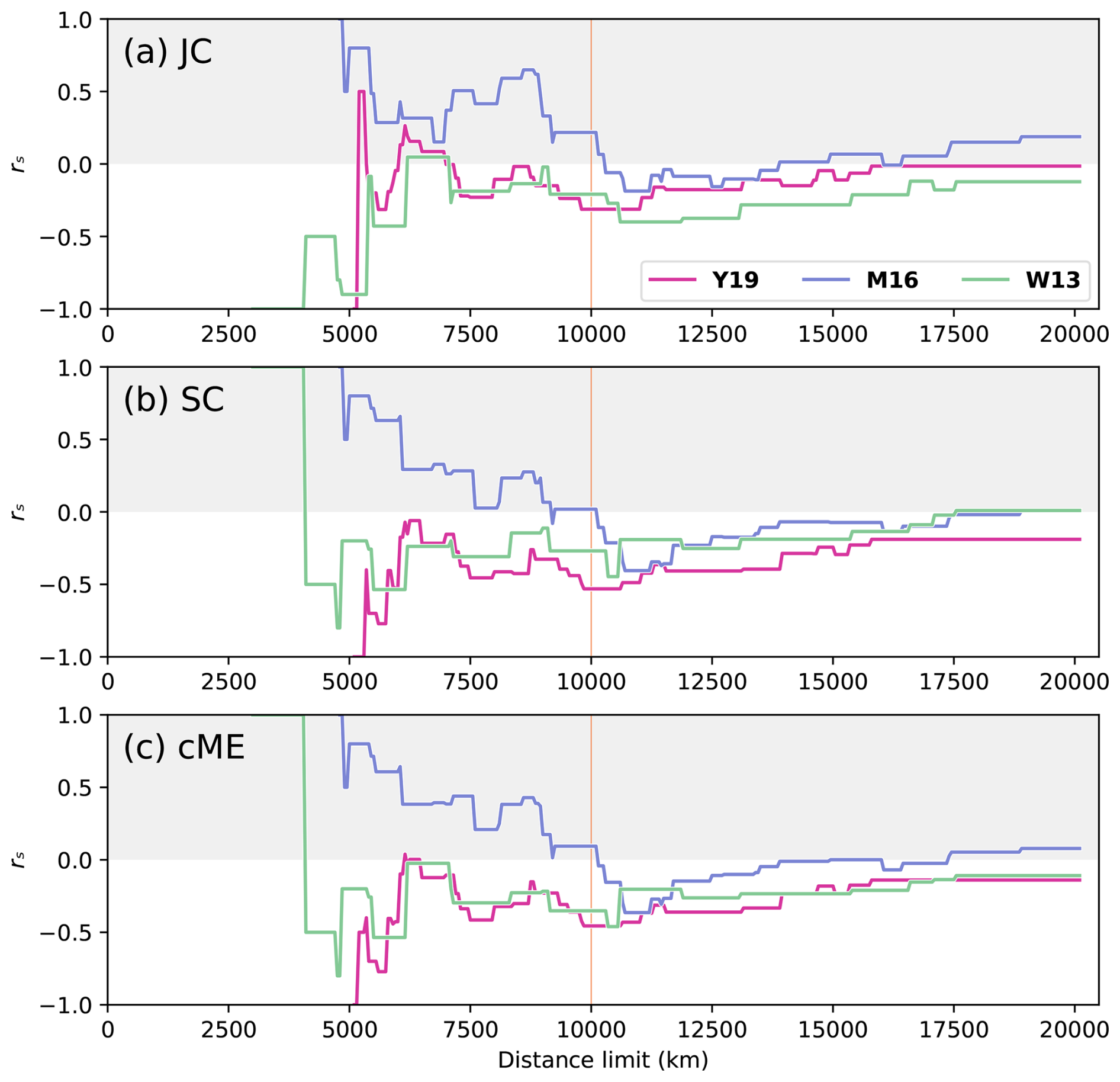
Figure 4 Spearman correlation coefficient r_s for all distance limits for each considered index, measuring the anti-correlation of genus-level biogeographic similarity and distance when comparing the SCB to all other plates with centroids located within the distance limits on the x axis (only plates within the distance limit were considered in the correlation) for Artinskian–Kungurian times, represented by reconstructions at 277 Ma. The grey region indicates positive correlations, meaning faunal similarity increases with physical distance, which is an unexpected trend. The vertical orange line at d_l = 10 000 km indicates the preferred distance limit.

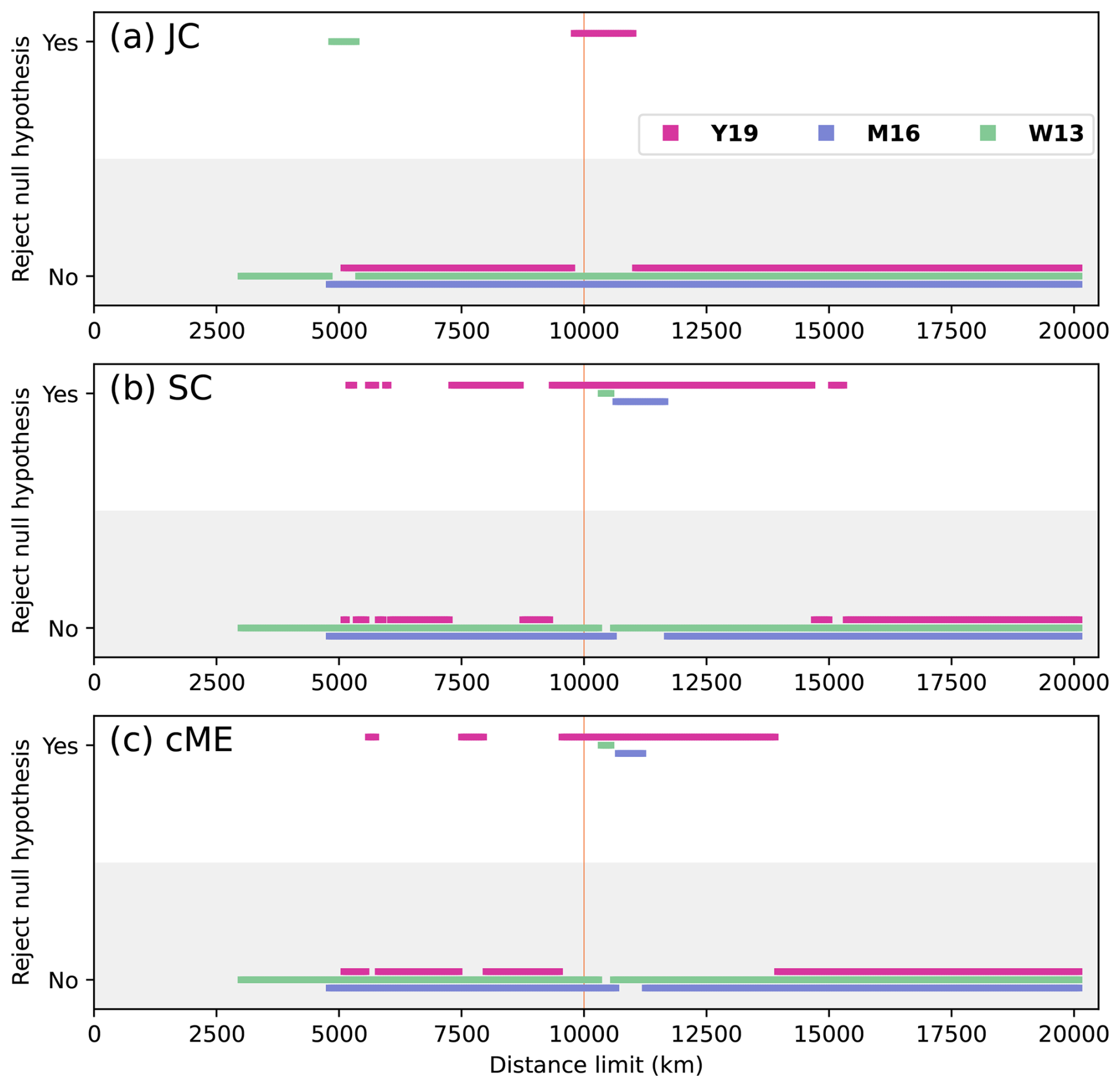
Figure 5 Statistical significance for all values of r_s presented in Fig. 4. A relationship is statistically significant (“Yes” in the graph) if the null hypothesis that faunal distribution is unrelated to physical distance between plates is rejected because the p value is less than 0.05. The vertical orange line at d_l = 10 000 km indicates the preferred distance limit.

4 Results

Comparing genus-level faunal similarity indexes between the SCB and all other plates in reconstruction Y19 revealed negative monotonic relationships for all three indices (Fig. 3). The correlation was strongest for index SC (r_s = −0.1895; Fig. 3b), followed by index cME (r_s = −0.1396; Fig. 3c) and a weak correlation for index JC (Fig. 3a). None of these relationships were statistically significant; however, they include distant plates for which the migratory distance for brachiopods is much larger than the measured distance, meaning that the results can be improved by imposing distance limits on the analysis. All possible distance limits were examined for the strength and statistical significance of correlations for each of the three reconstructions (Figs. 4 and 5).

The correlations between faunal similarity and physical distance are expected to be negative for all distance limits (white section of Fig. 4), which was the case for reconstructions Y19 and W13, where r_s was negative for > 90 % of all d_l for the Artinskian–Kungurian. For reconstruction M16, however, positive correlations (grey section of Fig. 4) were obtained for 47 % of all d_l. At smaller distance limits, all three reconstructions showed large instability in the relationship between faunal similarity and physical distance for each of the indices, with large fluctuations in r_s for small changes in d_l (Fig. 4). The relationship stabilized for all three reconstructions with all indices at larger distance limits (smaller fluctuations as new plates are added to the analysis), near d_l = 10 000 km for reconstruction Y19 and d_l = 11 000 km for reconstructions M16 and W13. Distance limits at or above those thresholds are most appropriate for further analysis. For indices SC and cME, reconstructions Y19 and W13 peaked at r_s⪅ −0.45 for d_l⪆ 10 000 km (Fig. 4b and c), while peaks for reconstruction M16 were at r_s≤ 0.4 for all indices. Index JC presented the overall weakest performance of all three faunal similarity indices, with none of the three considered reconstructions reaching r_s< −0.4 for any d_l > 10 000 km. While strong correlations were obtained for reconstructions Y19 and W13, it is important to ensure that the correlations are also statistically significant.

The statistical relationship between faunal similarity and physical distance was strongest for reconstruction Y19. There was consistent statistical significance for indices SC and cME at 10 000 km < d_l < 14 000 km (Fig. 5b and c). Statistical significance was lowest for index JC, with significance only for Y19 and 9800 km < d_l < 10 950 km (Fig. 5a). Statistically significant relationships occurred for some d_l for W13 and M16; however, the ranges for d_l which were statistically significant for reconstructions W13 and M16 were far smaller than the statistically significant d_l ranges for reconstruction Y19. Statistical significance also occurred for Y19 for correlations with greater distance limits than for the other two reconstructions, up to d_l = 10 950 km (JC), 15 300 km (SC), and 13 900 km (cME). These results suggest that the Artinksian–Kungurian longitude of the SCB in reconstruction Y19 is most consistent with the brachiopod biogeographic data among the three considered tectonic reconstructions. For reconstruction Y19, an optimal distance limit was determined at d_l = 10 000 km based on r_s and p as a function of d_l (Figs. 4 and 5).

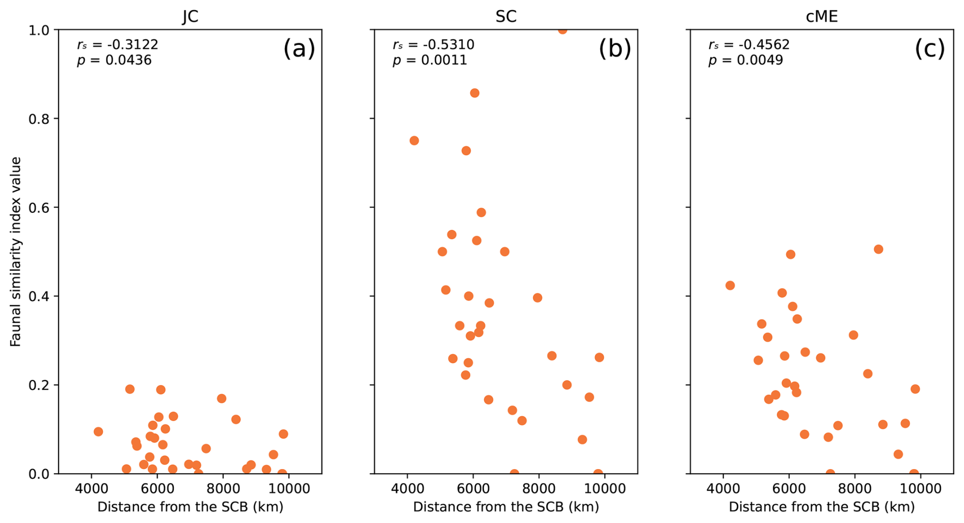
Figure 6 Relationships between genus-level faunal similarity and physical distance from the SCB for each index JC (a), SC (b), and cME (c), for 31 plates within d_l = 10 000 km of the SCB in reconstruction Y19 at 277 Ma, used to represent Artinskian–Kungurian times. The Spearman correlation coefficient r_s and p value are indicated on each subplot for each index.

A strong anti-correlation between faunal similarity and physical distance from the SCB was obtained for reconstruction Y19 with d_l = 10 000 km (Fig. 6) during Artinskian–Kungurian times. In detail, all three indices presented strongly negative and statistically significant correlations. The strongest correlation was obtained for index SC (r_s = −0.5310), which also exhibited the largest range of data, with points spread between a maximum of 1 and minimum of 0. Strong (r_s < −0.3) and statistically significant correlations were also obtained for indices JC and cME. These results show that there is a robust, statistically significant decrease in faunal similarity as distance increases from the SCB as it is positioned in reconstruction Y19 during Artinskian–Kungurian times.

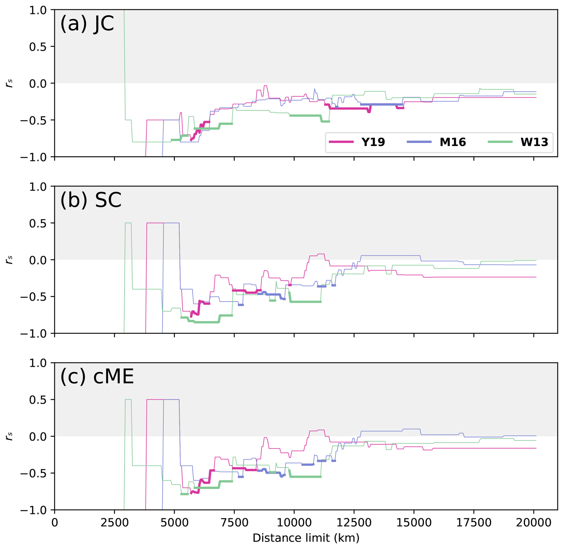
Figure 7 Faunal similarity and physical distance correlations for Asselian–Sakmarian times, represented using a reconstruction at 295 Ma. All three indices are presented for each reconstruction and all distance limits. Statistically significant r_s is shown as thick lines, while thinner lines represent statistically non-significant correlations.

The relationship between faunal similarity and physical distance during Asselian–Sakmarian times did not favour one reconstruction as strongly as the Artinskian–Kungurian results (Fig. 7). Similar to Artinskian–Kungurian times, there were large fluctuations in r_s with small changes in d_l for d_l⪅ 12 000 km for all reconstructions and indices. The most consistently statistically significant relationship occurred for reconstruction Y19 with index JC, which was statistically significant for 11 300 km < d_l < 14 550 km with a minimum r_s = −0.3923 and mean r_s = −0.3238 (Fig. 7a). This was the largest unbroken d_l range that is statistically significant during Asselian–Sakmarian times. For indices SC and cME, statistical significance was obtained most consistently for reconstruction W13 (Fig. 7b and c). This was primarily for lower d_l, with reconstruction W13 having no statistically significant correlations using d_l > 11 450 km for any index. Statistical significance was obtained least consistently for reconstruction M16, although statistical significance is obtained for index JC for 12 800 km < d_l < 14 500 km with r_s = −0.2840 (Fig. 7a).

5 Discussion

5.1 Position of the South China Block during Early Permian times

5.1.1 Artinskian–Kungurian times

The brachiopod fossil record is more consistent with the Artinskian–Kungurian location of the SCB in reconstruction Y19 than in reconstructions W13 and M16. This is indicated by strong, statistically significant negative correlations between faunal similarity and distance from the SCB for tectonic reconstruction Y19 (Figs. 4 and 5). The Artinksian–Kungurian location of the SCB in reconstruction Y19 effectively splits the Paleo-Tethys Ocean into two arms (Fig. 1a), in contrast to its position in the eastern margin of the ocean in reconstructions W13 and M16 (Fig. 1c and e).

Differences in the Artinksian–Kungurian locations of tectonic blocks isolated within ocean basins (e.g. North China, Amuria) between the considered tectonic reconstructions introduce some uncertainty in the results. As explained in more detail below, the main difference between reconstructions M16 and Y19 for Artinksian–Kungurian times is the location of the SCB (Fig. 1a, c, and e). Differences in the reconstructed location of other continental blocks affect the distances to the SCB and the relationships with biogeographic indexes. As such, the comparison between reconstruction W13 and reconstructions M16 and Y19 is less direct.

There are few differences in the geometry of Pangea between reconstructions M16 and Y19 (Fig. 1a and c), with the Siberian and Baltica blocks slightly further south-east in reconstruction Y19 compared to their locations in reconstruction M16. There are also differences in the location of smaller, isolated blocks. For example, Indochina and Amuria are reconstructed at slightly different distances from the SCB in reconstructions M16 and Y19. Although the North China Block is at similar distances from the SCB in reconstructions M16 and Y19, it is to the east of the SCB in reconstruction M16 and to the west of the SCB in reconstruction Y19. In the absence of other significant differences, the major cause of variation in the relationship between biogeographic indices and distance for reconstructions M16 and Y19 is expected to be the difference in distance of the SCB from Pangean circum-Tethyan blocks between the two reconstructions. Indeed, the SCB is roughly 4000 km further from the east Pangean coastline (comprised primarily of Baltica and the Cimmerian terranes), 2000 km further from the Cimmerian terranes, and 1000 km closer to the Australian continental block in reconstruction M16 than in reconstruction Y19 (Fig. 1a and c).

The SCB is reconstructed further to the south-west in reconstruction W13 than in reconstruction M16, and it is reconstructed significantly further to the south-east of its location in reconstruction Y19 (Fig. 1a, c, and e). Even though the locations of the SCB are closer between reconstructions W13 and M16 than between reconstructions W13 and Y19, the correlation results are more similar between reconstructions W13 and Y19 than between reconstructions W13 and M16 (Fig. 4). This result is likely due to other major differences in global paleogeography between reconstruction W13 and reconstructions M16 and Y19 (Fig. 1a, c, and e). The Cimmerian terranes are separated from Pangea and further to the north-east in reconstruction W13, which changes their distribution from the SCB from almost equidistant (the Cimmerian terranes are about 6000 km away from the SCB in reconstruction Y19 and 8000 km away from the SCB in reconstruction M16; Fig. 1a and c) to mostly radially distributed (from about 500 km to about 8000 km away from the SCB in reconstruction W13; Fig. 1e). The northern Pangean blocks (Siberia and Baltica) are further to the south-east and North China and Amuria are further to the south (such that North China borders the SCB) in reconstruction W13 than in reconstructions M16 and Y19. These differences may cause the distance to the SCB for many plates to be more similar between reconstructions W13 and Y19 than between reconstructions W13 and M16 (Fig. 4). The different relationships between biogeographic indexes and distance for reconstructions W13 and Y19 (Figs. 4 and 5) are due to different distances between the SCB and other plates, including the Cimmerian terranes (see above); the North China Block, which is approximately 4000 km away from the SCB in reconstruction Y19 but adjacent to it in reconstruction W13; Baltica, which is 5000 km away from the SCB in reconstruction Y19 and 7000 km away in reconstruction W13; and the Australian Block, which is 4000 km from the SCB in reconstruction W13 and 6000 km from the SCB in reconstruction Y19. It is important to consider that the SCB in reconstruction W13 differs from the reconstruction Y19 and M16 positions for the SCB not only longitudinally but also latitudinally. This, along with the different set of tectonic blocks compared to Y19 and M16, means that we cannot consider this as purely a comparison and constraint for SCB longitude. Nevertheless, this remains valuable as a comparison for the overall suitability of the SCB location within the global tectonic configuration of W13 compared to Y19 and M16.

5.1.2 Asselian–Sakmarian times

There is no clear result indicating which reconstructed SCB location is most favoured by the brachiopod faunal distribution during Asselian–Sakmarian times (Fig. 7). Statistical significance was most consistently obtained for reconstruction W13; however, many of these statistically significant relationships were for short distance limits for which the relationship was inconsistent (Fig. 7). Statistically significant relationships were consistently obtained for reconstruction Y19 using index JC for large distance limits (Fig. 7a); however, this is not reproduced for indices SC and cME, for which r_s was low without statistical significance for large distance limits. For Asselian–Sakmarian times, the weakest overall relationship between faunal similarity and physical distance from the SCB was obtained for reconstruction M16. For reconstructions Y19 and M16, there are only minor changes in plate tectonic locations between 295 and 277 Ma (Fig. 1a–d). There are small changes in location for the other isolated Tethyan plates and minor movement of the SCB between 295 and 277 Ma in reconstruction M16, but the Pangean coastline remains quite similar between the two time steps for both reconstructions. There is greater movement of tectonic blocks between the two time steps for reconstruction W13, in particular the Cimmerian terranes separate from Pangea (Fig. 1e and f). Regardless of these changes in global plate configuration for any of the three reconstructions, plates are encountered in a very similar order at both 295 and 277 Ma. This means that the Spearman correlation should remain similar to what was obtained for Artinskian–Kungurian times. The lack of clear relationships for any of the reconstructions is likely a result of the smaller fossil dataset for Asselian–Sakmarian times (4670 occurrences) than for Artinskian–Kungurian times (9988 occurrences) and differences in the distribution of these fossils.

There are some noteworthy changes in fossil distribution for Tethyan tectonic plates between 277 and 295 Ma. Indochina, the closest plate to the SCB, presents over 40 genera during Asselian–Sakmarian times, but not a single fossil occurrence is attributed to the plate during Artinskian–Kungurian times (Fig. 1). There are also 65 % more genera for North China and 30 % more genera for the northern Cimmerian terranes during Asselian–Sakmarian times compared to Artinskian–Kungurian times. Conversely, Amuria records over 40 genera during Artinskian–Kungurian times but only 7 during Asselian–Sakmarian times, and Kunlun–Alashan records 20 genera during Artinskian–Kungurian times compared to 0 during the Asselian–Sakmarian times. Additionally, there are 65 % more genera on the Tarim Block and 25 % more genera on the southern Cimmerian terranes during Artinskian–Kungurian times than during Asselian–Sakmarian times (point densities between the two columns in Fig. 1). These differences in fossil distribution between the two time periods are expected to have the greatest biogeographic connection with the SCB, as they are for blocks in the same ocean basin as the SCB. The small sample sizes on these blocks during Asselian–Sakmarian times than during Artinskian–Kungurian times weaken the power of the statistical testing to determine a relationship (VanVoorhis and Morgan, 2007). Results may be improved by expanding the dataset for Asselian–Sakmarian times by considering more marine phyla in the analysis (rather than just Brachiopoda), which could be done with the framework introduced for this analysis.

5.2 Limitations and possible future improvements

5.2.1 Statistical significance

The fossil record is known to be incomplete, although the degree to which this impacts studies based on fossil data is debated (Benton et al., 2000). Preservation biases lead to differential preservation of biota between different environments so that regions in which large numbers of sedimentary rocks are deposited are more favourable for fossil preservation. Regions preserving Early Permian sedimentary rocks may preserve greater proportions of the regional biota, as the volume of marine sedimentary rock is positively correlated with biodiversity (Crampton et al., 2003; Raup, 1976). Observed variations in biodiversity have also been linked to the number of people working on sampling for a region (Sheehan, 1977), with a larger number of workers in a given region leading to more discovery of specimens. This causes larger biota datasets to be known for developed regions (as is clear from Fig. 1, in which the greatest point densities occur in present-day North America, Europe, China, and Australia). Such biases are likely to cause apparent differences in biodiversity between regions that are not representative of true faunal assemblages. These sampling biases inherent to fossil data can make it difficult to effectively determine relationships; however, increasing the sample size makes the sampled distribution more closely resemble the true distribution, thus reducing the impact of sampling errors on the statistical test (Särndal et al., 2003).

Statistical significance could generally be established for greater distance limits (Fig. 5): increasing the distance limit increases the sample size, which increases the power of the statistical test to identify a relationship (VanVoorhis and Morgan, 2007). This is clear from the calculation of the t statistic that is used to determine the p value:

$$\begin{array}{}\text{(4)}& t=r_{\mathrm{s}}\sqrt{{\displaystyle \frac{n-\mathrm{2}}{\mathrm{1}-r_{\mathrm{s}}^{\mathrm{2}}}}},\end{array}$$

where n is the sample size, meaning that t is proportional to n. The probability density function for t is a bell-shaped curve centred about 0 (Kokoska and Zwillinger, 2000). The area under this curve from $t\stackrel{\mathrm{\infty }}{⟶}$ gives the p value; thus, as $\left|t\right|$ increases, the p value decreases (Kokoska and Zwillinger, 2000), meaning that when r_s is kept constant, the power to determine statistical significance increases with sample size n (Eq. 4). This explains why there are many cases in which r_s values may be very similar for reconstructions W13 and Y19, but the correlation for reconstruction Y19 is statistically significant, whereas the correlation for reconstruction W13 is statistically non-significant. For all d_l > 5500 km, the sample size was greater for reconstruction Y19 than for reconstruction W13 (Fig. 2a), giving the statistical test greater power to identify a relationship.

Figure 8 Relationship between faunal similarity and physical distance based on taxonomic data at the family level during Artinskian–Kungurian times (reconstructed at 277 Ma). Results selected based on success: (a) r_s for index SC, all reconstructions, and all distance limits; (b) statistical significance for index SC, all reconstructions, and all distance limits; and relationships between faunal similarity and physical distance from the SCB for each index JC (c), SC (d), and cME (e), for 31 plates within d_l = 10 000 km of the SCB in reconstruction Y19.

5.2.2 Taxonomic level

In order to check any impact of possible biases in taxonomic identification of the fossil records, we analysed the same dataset at the family level. This effectively tested the sensitivity of the developed framework to changes in taxonomic rank of the input data. The relationships between family-level similarity and physical distance from the SCB for Artinskian–Kungurian times (reconstructed at 277 Ma) corroborate the SCB position for reconstruction Y19 as the most supported by faunal data (Fig. 8). The strong correlation between faunal similarity and physical distance for reconstruction Y19 maintains statistical significance across nearly 70 % of distance limits and for all d_l > 6250 km (Fig. 8b). While index JC is not statistically significant at d_l = 10 000 km (Fig. 8c), indices SC and cME both presented stronger relationships than were obtained at the genus level (r_s = −0.5670 and r_s = −0.4559, respectively; Figs. 8d and e). This result is consistent with the genus-level outcome, which indicates that there would be an insignificant impact of taxonomic biases in our results. It also shows that the framework is robust to changes in taxonomic ranks.

5.2.3 Faunal provinciality

Environmental variation across continental blocks can lead to multiple distinct biogeographic regions on a single block. The methods used in this study may lead to inaccuracies when biogeographic regions are selected that are far beyond the distance limit or when multiple regions that should be distinct become combined as one coherent region. This problem is exacerbated in reconstruction W13, which presents a smaller number of plates and a larger area covered by each plate. Alternate methods to measure distance and define biogeographic regions may be implemented in future work to improve the method used in this study. Rather than selecting plates within a distance range, distances between each fossil occurrence and the SCB could be measured, with only occurrences within the distance limit being selected. This may separate distinct biogeographic regions on large plates, but it could also split blocks (e.g. the Cimmerian terranes in M16; Fig. 1c). Multivariate statistical methods, such as ordination and cluster analysis (Shi, 1993), are other interesting possibilities to address this issue in future improvements of the framework introduced in this study. These methods may allow for greater resolution in defining biogeographic regions by identifying locations that should be distinct regions rather than defining each region as the entire tectonic block. It has also been suggested that an open-ocean distance of 1400 km may be required between islands to develop a distinct faunal province (Shi, 1996). Taking such factors into account would potentially improve results for both large plates with multiple faunal provinces and clusters of islands comprised of individual tectonic blocks that may not be distinct faunal provinces.

All three reconstructions primarily differed in the longitude of continental configurations, with continental blocks having similar latitudes across each reconstruction (Fig. 1). Continental blocks were in the same biogeographic realms across each reconstruction, as they are defined latitudinally (Waterhouse and Bonham-Carter, 1975; Shen et al., 2013), implying that the reconstructions should all be affected equally by faunal provinciality. Reconstruction W13 places the SCB in the Southern Hemisphere (Fig. 1e and f), whereas reconstructions M16 and Y19 place it in the Northern Hemisphere (Fig. 1a–d). Despite this discrepancy, the SCB remains within warm-water biogeographic realms, suggesting that latitudinal climate variations should not have a major effect on the results.

5.2.4 Limitations inherent to each of the three considered biogeographic indexes

Index JC measures the true similarity between two sets of fossil occurrences and is less reliable if the real biodiversity is unknown, which is likely the case with paleontological data. Indeed, the validity of index JC in paleobiogeographic studies is questionable (Simpson, 1960). The use of the union between two sets of fossil occurrences is problematic when one set is much larger than the other; incidentally, the SCB is one of the largest biota sets for Early Permian brachiopods, with nearly 150 genera present on the SCB, 3–7 times larger than the average number of genera per plate that the SCB is compared to (Fig. 2b). This is highlighted by the ideal index values (Fig. 6), where the maximum values for index JC are 0.19 compared to 1 (for index SC) and 0.51 (for index cME). This reduced range of values for index JC makes the determination of a linear relationship less effective (da Silva and Seixas, 2017); however, the use of the Spearman rank correlation alleviates this issue.

Index SC was developed to extrapolate the true similarity by assuming that biodiversity is constant across regions (Simpson, 1960); thus, the calculation is limited by the smaller region. This risks overestimating the true similarity if there are real differences in biodiversity, and it is susceptible to large variations in value from small variations in set intersection when the smaller biota set is small. Index cME is limited by both of the issues that exist for indexes JC and SC; however, averaging each endemism ratio reduces the impact of each limitation. The Raup–Crick index (Raup and Crick, 1979), which considers how widespread each genus is across a given faunal assemblage and compares similarity between observed sets to similarity between randomly generated sets, could be used in future work, as it has shown promise (Schmachtenberg, 2008).

Each of the three indices considered in this study and the relationship to physical distance are subject to real-world complications in the relationship that they measure, typically due to factors such as land barriers, which lead to migration distances that are much greater than measured physical distances. This is clearest for the connection between the SCB and North America (Fig. 1), where brachiopods are located on the eastern coast, implying that migratory pathways require travel either across the Panthalassan Ocean or north around Siberia. This leads to strong family-level faunal similarity (Waterhouse and Bonham-Carter, 1975), as North America and the SCB occupy the same Paleoequatorial region, but limited genera-level similarity, due to substantially limited brachiopod dispersal across the Panthalassan Ocean. This is in contrast to the physical distance, as measured by PyGPlates, which is directly across the Paleo-Tethys Ocean and a much shorter distance than the actual dispersal pathway (Fig. 1). This is supported by the lack of statistical significance for genus-level similarity in reconstruction Y19 at the longest distance limits (Fig. 4). Nevertheless, statistically significant results were obtained at the largest distance limits when using family-level similarity.

5.2.5 Possible interdependence of the considered datasets

While the Early Permian location of the SCB was determined independently of faunal data in reconstructions W13, M16, and Y19, all three reconstructions used faunal data in the constraint of other tectonic blocks. Faunal data were used to constrain the location of the Australian Block by interpreting paleoenvironments in reconstruction W13 (Wright et al., 2013), so that results may not be entirely independent for that plate. In contrast, faunal affinity was only used to determine connected tectonic plates during Devonian times in reconstruction M16 (Matthews et al., 2016) and to determine that two plates were separate micro-continents at the Silurian–Devonian boundary in reconstruction Y19 (Young et al., 2019). We note that the dispersal of brachiopod larvae depends on ocean currents (Lam et al., 2018) as well as larva types (Williams et al., 1996; Carlson, 2016) and that ocean currents depend on the location of the SCB and other tectonic blocks in each of the considered tectonic reconstructions (Fig. 1).

The method used to constrain the location of the SCB in M16 is also problematic, as it assumes that large low-shear-velocity provinces (basal mantle structures) have remained stationary at least since the emplacement of the Emeishan LIP (Domeier and Torsvik, 2014), which is unnecessary given that mantle flow models that predict mobile basal mantle structures are consistent with the record of large volcanic eruptions (Flament et al., 2022; Bodur and Flament, 2023; Cucchiaro et al., 2025).

5.3 Comparison to previous work and possible future directions

Similar quantitative methods have been used to assess relationships between biogeographic indexes and distance (Shi, 1993; Angiolini, 2001; Lees et al., 2002; Belasky et al., 2002; Shen et al., 2013), although on smaller spatial scales. Improved data availability and analytical tools have made these quantitative methods applicable at the global scale. Here, the SCB was compared to all other tectonic plates, rather than to a selection of geographically close plates. Comparison to a small number of plates makes it possible to define a relative position within a region, whereas comparison to all other plates makes it possible to elect a preferred location relative to global geography.

This work could be extended by testing more reconstructions of Early Permian tectonic plate configuration. Recent reconstructions of the configuration of Tethyan blocks during Early Permian times using faunal affinity suggest significantly different Tethyan arrangements than any of the three reconstructions tested in this study (Xu et al., 2022, 2024). In particular, the three reconstructions tested here show minimal separation of the Cimmerian terranes from Gondwana at 277 Ma, while faunal affinity suggests that some Cimmerian terranes may have separated from Gondwana during Artinskian times and been located much closer to the SCB at 277 Ma (Xu et al., 2022, 2024). In contrast, for Asselian–Sakmarian times, the Cimmerian terranes are reconstructed to similar positions based on faunal affinity (Xu et al., 2022, 2024), as they are in the reconstructions considered in this study (Fig. 1b, d, and f). Testing these differing configurations would be a valuable addition to this work; however, it is not currently possible, as reconstructions based on faunal affinity (Xu et al., 2022, 2024) only exist as series of static paleogeographic reconstruction maps, rather than as continuous plate tectonic reconstructions compatible with PyGPlates.

The framework developed here could be used to systematically evaluate the compatibility of tectonic reconstructions with faunal data, or it could be applied to other fields of study such as paleo-oceanography. The framework is highly adaptable and can be applied to any reconstruction, geological period, and faunal dataset that provides location data. For example, in this contribution, we presented sensitivity analyses for distinct ages and taxonomic levels. Paleobiogeography has been used successfully as a qualitative method to track past ocean currents (Harper et al., 2005), and the framework introduced in this study opens the opportunity to extend these past works quantitatively and to larger scales. Testing tectonic plate locations could also be applied beyond single tectonic plates, as was done here, by testing faunal affinity for all tectonic plates against all other tectonic plates across geological times. The framework could also be extended to any suitable fossil type. In principle, it should be possible to design a framework in which distances between all tectonic blocks would be a function of faunal similarity, which is one of the observations that led to the establishment of tectonic reconstructions (Jell, 1974). In such a framework, faunal data would be considered to be one method of constraint and validation for plate tectonic configuration alongside other, independent constraints such as paleomagnetic and stratigraphic data.

6 Conclusions

We assessed the Early Permian longitude of the SCB using a new framework to evaluate the global relationship between faunal similarity and tectonic distance. We determined that the Artinskian–Kungurian position of the SCB in the reconstruction of Young et al. (2019) is more consistent with the brachiopod distribution than the Artinskian–Kungurian position of the SCB in the reconstruction of Wright et al. (2013) and Matthews et al. (2016). The strength of correlation between faunal similarity and physical distance between the SCB and circum-Tethyan tectonic blocks was largest for Y19. This implies that the SCB could have been positioned centrally within the Paleo-Tethys Ocean at 103° E, which is 20–30° further west than in the reconstructions of Wright et al. (2013) and Matthews et al. (2016) that place the SCB on the margin of the ocean. This likely has important implications for Paleo-Tethys Ocean circulation and for reconstructions of paleoclimate change throughout Early Permian times. While the analysis of the position of the SCB during Asselian–Sakmarian times was inconclusive, it showcases the flexibility of the framework introduced in this contribution. This highlights that the presented framework could be valuable to future studies of paleogeography, as it can be extended to refine global tectonic plate locations based on faunal data.