Colored dissolved organic matter (CDOM) alters the seasonal physics and biogeochemistry of the Arctic Mackenzie River plume

Arctic warming affects land-to-ocean fluxes of organic matter through increased permafrost thaw, coastal erosion or river discharge, with significant impacts on coastal ecosystems and air-sea CO₂ fluxes. In this study, we modify a regional version of the Estimating the Circulation and Climate of the Ocean model coupled to the Darwin ocean biogeochemistry module (ECCO-Darwin) to simulate Mackenzie River export of colored dissolved organic matter (CDOM) and its effect on light attenuation, marine carbon cycling, and water-column heating from UV-A to visible light absorption. We find that CDOM light attenuation triggers both a two-week delay in the seasonal phytoplankton bloom and an increase in sea-surface temperature (SST) by 1.7 °C. While the change in phytoplankton phenology has limited effect on air-sea CO₂ fluxes, the local increase in SST due to terrestrial organic matter input switches the coastal zone from an annual sink of atmospheric CO₂ to a source (7.35 Gg C yr⁻¹). Our work suggests that the projected increase in terrestrial CDOM has strong implications for phytoplankton phenology and coastal air-sea carbon exchange in the Arctic.

1 Introduction

As anthropogenic emissions of carbon dioxide (CO₂) continue to increase (IPCC, 2023), it is critical to understand the time variability and future trajectory of the ocean carbon sink and its regional-scale response. The Arctic Ocean (AO) region constitutes an important sink of atmospheric CO₂, estimated to be 116 ± 4 Tg C yr⁻¹ (Yasunaka et al., 2023), or roughly 7 % of the global-ocean sink (Roobaert et al., 2019). When focusing on coastal regions, the AO contribution constitutes up to 46 % of the global sink (Dai et al., 2022). The intense cooling of inflowing waters from adjacent seas and favorable conditions for phytoplankton growth result in elevated CO₂ uptake from increased CO₂ solubility and biological consumption, respectively. With Arctic air temperatures rising three to four time faster than the global mean due to the ice-albedo feedback (Rantanen et al., 2022), retreating sea ice cover allows for a larger ocean surface area to be exposed to sunlight for longer periods of time (Bliss et al., 2019; Ardyna and Arrigo, 2020). As a result, AO Net Primary Production (NPP) increased by 90 Tg C (38 %) from 1998–2012 (Ardyna and Arrigo, 2020; Lewis et al., 2020). Additionally, recent work by Terhaar et al. (2021) showed that a third of AO primary production is sustained by terrestrial fluxes from coastal erosion and rivers, resulting from large lateral fluxes of carbon and nutrients (Dittmar and Kattner, 2003; Le Fouest et al., 2013; Nielsen et al., 2022). However, the quantity and the composition of terrestrial matter exported to coastal regions is also impacted by climate change (Bertin et al., 2022; Mann et al., 2022; Tank et al., 2023), with potential to affect the biophysical conditions of coastal AO waters.

As Arctic river freshwater discharge increases (Feng et al., 2021), the quantity of terrestrial dissolved organic matter (DOM) exported to AO coastal peripheries is expected to increase. Due to complex molecular composition including aromatic cycles, DOM chemical composition depends on its origin and encompasses more than 20 000 molecular formulae (Dittmar et al., 2021). As it transitions from land to ocean, microbial activity and light alter DOM molecules, with their chemical composition being highly dependent on the transit through the terrestrial-aquatic environment (Cory et al., 2014; Cory and Kling, 2018). Once in coastal waters, the composition of riverine-derived DOM varies seasonally, likely being more labile (i.e., more easily degraded by microbes) during spring freshet (Spencer et al., 2009). A fraction of DOM, termed colored DOM (CDOM), possesses unique optical characteristics that enable it to efficiently absorb shortwave radiation – from ultraviolet (UV) to the visible light spectrum. In Arctic rivers, CDOM molecular weight and aromaticity increases with discharge (Mann et al., 2016), rendering it more resistant to degradation by marine bacteria (i.e., more refractory). Simultaneously, its interaction with light transforms CDOM either (1) into more-labile components of DOM (Osburn et al., 2009; Cory and Kling, 2018) or (2) directly into Dissolved Inorganic Carbon (DIC; Bélanger et al., 2006; Aarnos et al., 2018), which can promote CO₂ outgassing. By dampening light penetration into the water column, CDOM can impact primary production (Li et al., 2024; Berezovski et al., 2025) and upper-ocean temperature (Hill, 2008; Kim et al., 2016; Soppa et al., 2019), which can also modulate air-sea CO₂ exchange. Consequently, the magnitude of air-sea CO₂ flux in AO river plume regions remain highly uncertain, with both local-to-regional outgassing or uptake observed (Terhaar et al., 2019; Bertin et al., 2023; Roobaert et al., 2024). Additionally, as a result of global warming, accelerating permafrost thaw has the potential to change the composition of organic matter in coastal waters and therefore the coastal air-sea CO₂ fluxes via increased coastal erosion (Tanski et al., 2021; Nielsen et al., 2024) or river discharge (Mann et al., 2022). Thus, by a cascading effect, CDOM can locally amplify sea ice melting due to increased sea-surface temperature (SST) from increased light attenuation (Pefanis et al., 2020). Therefore, understanding how terrestrial CDOM biophysical feedbacks influence coastal waters is critical to better characterize the consequences of climate change across Arctic coastal peripheries.

In AO coastal regions, NPP remains highly uncertain. The harsh polar conditions make it challenging to collect in-situ observations and estimates from remote sensing are often contaminated by sea ice, clouds, low light levels, and the high proportion of CDOM light absorption (Lewis and Arrigo, 2020; Li et al., 2024). Estimating NPP remotely also requires several key assumptions regarding the vertical distribution of phytoplankton, since satellites only capture near-surface data (Arrigo et al., 2011; Silsbe et al., 2016). Current estimates suggest AO NPP ranges from 203–516 Tg C yr⁻¹ (Bélanger et al., 2013; Arrigo and Van Dijken, 2015), but these values are likely overestimated in coastal regions due to high CDOM concentrations. As a result, satellite estimates of air-sea CO₂ flux often fail to capture nearshore, river-plume regions (Bertin et al., 2023). To complement remote sensing, ocean biogeochemistry models (OBMs) permit full space-time coverage of AO coastal regions and can provide a mechanistic understanding of the processes that govern the air-sea CO₂ flux (Manizza et al., 2019; Mathis et al., 2022). Yet while most regional-scale OBMs now incorporate land-to-ocean nutrient transport (Terhaar et al., 2019; Lacroix et al., 2021; Savelli et al., 2025), their representation of the intricacies due to the CDOM feedbacks described above often remains partial or completely absent (though see e.g. Kim et al., 2018; Gnanadesikan et al., 2019; Pefanis et al., 2020).

In this study, we utilize a regional ocean-sea-ice-biogeochemistry model (ECCO-Darwin) to examine how riverine CDOM impacts the seasonal cycle of phytoplankton biomass, primary production, and carbon cycling in the coastal AO. Our objectives are to (1) separate and explicitly quantify how CDOM's light attenuation properties affect both the physics and biogeochemistry in the river plume and (2) estimate how riverine CDOM modulates coastal air-sea CO₂ flux. Here, we focus on the Southeastern Beaufort Sea (SBS), where the Mackenzie River discharges substantial freshwater and DOM into the AO (Bertin et al., 2022; Juhls et al., 2022). The remainder of this paper is structured as follows. First, we describe improvements made to the existing ECCO-Darwin regional configuration of the Southeastern Beaufort Sea (ED-SBS) regional set-up (Run_strat in Bertin et al., 2025) to incorporate CDOM processes and add riverine CDOM forcing. Second, we analyze the seasonal bio-physical conditions simulated by ED-SBS in the Mackenzie River plume. Third, we assess the impact of riverine CDOM on the physical characteristics of the plume region. Fourth, we analyze changes in phytoplankton phenology driven by riverine CDOM. Fifth, we estimate how CDOM impact the air-sea CO₂ flux within the plume region. Finally, we provide concluding remarks and suggestions for future work.

2 Methods

2.1 Explicit CDOM tracer parameterization

To simulate the coastal AO environment, we used the ED-SBS regional configuration, whose general numerical characteristics are fully detailed in Sect. S1 in the Supplement and in Bertin et al. (2023, 2025). ED-SBS explicitly simulated four plankton functional types (PFTs) representative of ecosystems in the AO (diatoms, large eukaryotes, and small and large zooplankton), along with phytoplankton Chlorophyll a (Chl a) concentration. Two marine dissolved organic carbon (DOC) pools are simulated with chemical properties representative of those found in the coastal AO: a semi-refractory pool (DOC_sr) characterizing the long-residence-time carbon loop with a lifetime of τ = 10 years (Manizza et al., 2009), and a semi-labile pool (DOC_sl) characterizing the short-residence-time carbon loop with a lifetime of τ = 1 month (including DOC molecules characterized by turnover rates ranging from weeks to months; Holmes et al., 2008; Spencer et al., 2015; Bertin et al., 2025). Land-to-sea forcing included daily discharge of freshwater and 6 biogeochemical tracers from the Mackenzie River, distributed over the three major Mackenzie Delta outlets: Shallow Bay (29.8 %), Beluga Bay (37.6 %), and Kugmallit Bay (32.6 %) (Morley, 2012; Bertin et al., 2022). Freshwater discharge was driven by daily gauge measurements from the Arctic Great River Observatory (ArcticGRO; McClelland et al., 2023) and was linked to daily river temperature obtained from the Tokuda et al. (2019) dataset. Riverine concentrations of DOC, dissolved organic nitrogen (DON), dissolved organic phosphorus (DOP), dissolved silicate (DSi), dissolved inorganic carbon (DIC), and alkalinity (Alk) were forced as detailed in Bertin et al. (2025). As each export of dissolved organic constituents (DOC, DON & DOP) are estimated independently, the terrestrial dissolved organic matter pool is not constrained by a constant $\mathrm{C}:\mathrm{N}:\mathrm{P}$ ratio such as in Terhaar et al. (2019), Gibson et al. (2022), Bertin et al. (2023).

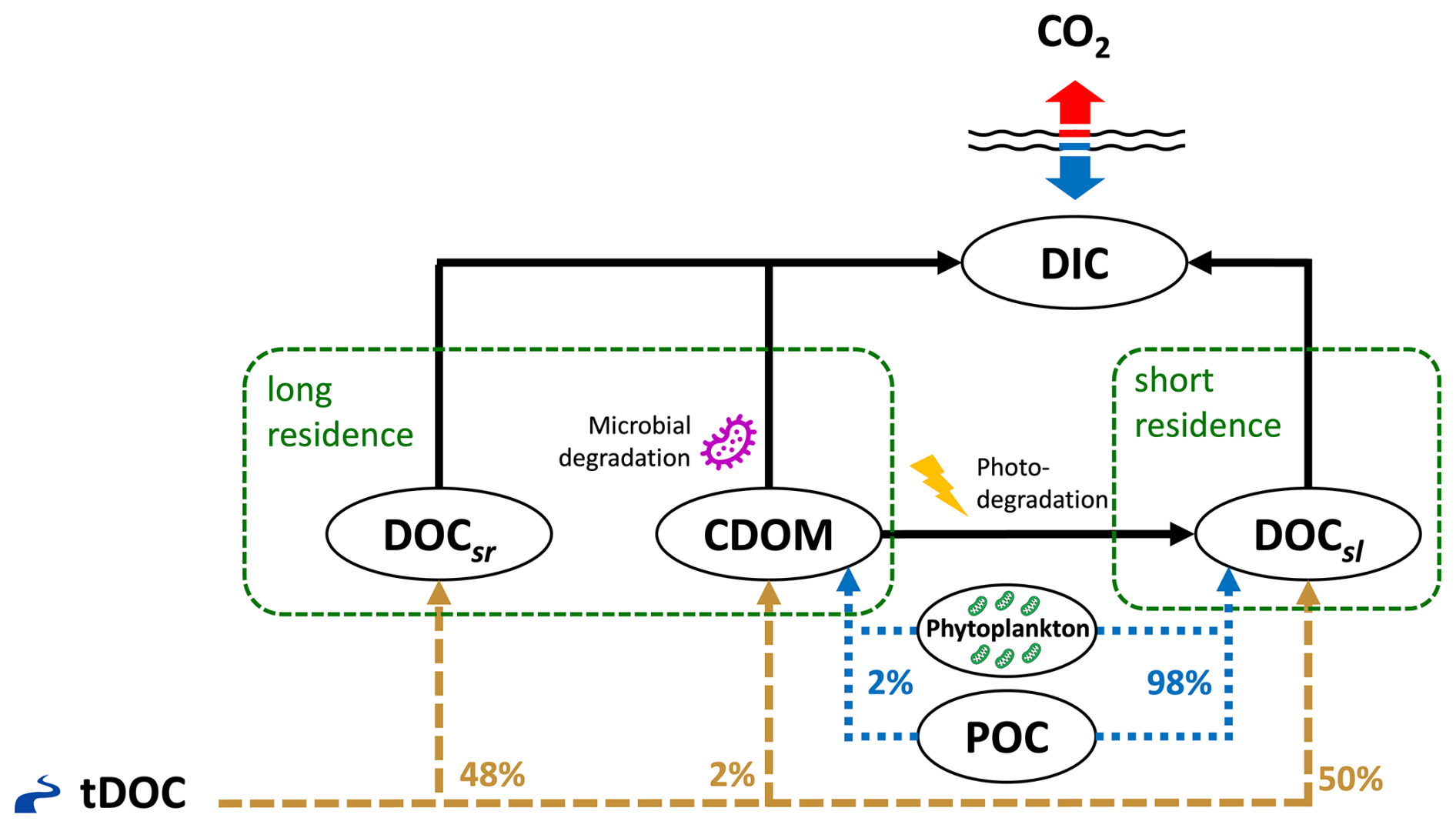
Figure 1 Conceptual diagram of dissolved carbon mass fluxes in the ED-SBS model. The Mackenzie River terrestrial DOC (tDOC) mass flux (dashed brown lines) is distributed into marine DOC and CDOM pools according to the percentages shown in brown text. The result of phytoplankton grazing/mortality and particulate organic carbon (POC) dissolution is distributed over the DOC_sl and CDOM pools (dotted blue lines).

In this study, we added an explicit “CDOM-like” tracer to ED-SBS, expressed as a carbon mass concentration (mmol C m⁻³), following the schematic shown in Fig. 1. Terrestrial CDOM, which is observed to be non-labile (Blough and Del Vecchio, 2002; Aarnos et al., 2018), was added to the long-residence-time carbon loop of the model using the same microbial turnover time as DOC_sr (τ = 10 years). The CDOM tracer also interacted with the short-residence-time carbon loop by photochemical alteration of CDOM into more-labile carbon (Ward et al., 2017; Grunert et al., 2021; Clark et al., 2022). CDOM was photodegraded into DOC_sl with a maximum bleaching turnover time of 6 d (Dutkiewicz et al., 2015), which was modulated by light intensity. Bleaching rate linearly increased from 0 when light intensity is 0 W m⁻² to a maximum value (0.167 d⁻¹) when light is above 13 W m⁻² (Dutkiewicz et al., 2015). CDOM photodegradation rate corresponds to the bleaching rate modulated by a temperature function. When degraded into DOC_sl, CDOM products DON and DOP followed the molar ratio of $\mathrm{120}:\mathrm{16}:\mathrm{1}$, allowing to represent the additional nutrient input generated by organic matter consumption – Redfield ratio is used due to a lack of data regarding CDOM photodegradation products. A fraction f_CDOM (=2 %) of mass fluxes received by DOC_sl through phytoplankton grazing/mortality and particulate organic carbon (POC) dissolution was also redistributed to CDOM.

In ED-SBS, the Mackenzie River terrestrial DOC (tDOC) mass flux was equally distributed (50 %) between semi-labile (DOC_sl) and semi-refractory (DOC_sr) DOC pools (based on recent estimates of the bioavailable tDOC fraction in the SBS, Fabien Joux, unpublished data from Nunataryuk field campaign; Tisserand et al., 2021; Lizotte et al., 2023). While 97 % of DOC concentration variance is explained by CDOM absorption (Matsuoka et al., 2012), the mass concentration of riverine CDOM exported to SBS coastal waters remains unknown. As CDOM is part of the long-residence-time loop, we redistributed a percentage of tDOC mass flux from DOC_sr into the CDOM pool. After a sensitivity analysis (detailed in Appendix B), we set the ratio to 2 % – re-partitioning Mackenzie River tDOC mass flux into 50 %, 48 %, and 2 % DOC_sl, DOC_sr, and CDOM, respectively. Our ratio of total tDOC exported as CDOM falls in the lower range of estimates for the top 10 DOC exporting rivers (4 %–38 % of tDOC; Aarnos et al., 2018). Finally, we generated CDOM initial and boundary conditions following the methods detailed in Sect. S2.

2.2 CDOM light attenuation relationship

We first developed a new method for simulating CDOM light attenuation across the shortwave spectrum, from 320–735 nm. This allowed us to resolve the physical effect of CDOM light attenuation occurring in the UV-A (320–400 nm) and in the visible (400–735 nm) bands; the latter is often associated with Photosynthetically Active Radiation (PAR; spanning from 400–700 nm). An analysis of 31 CDOM spectral absorption measurements taken during the 2009 Malina campaign for different CDOM conditions across the SBS (see sampling locations in Fig. S1 in the Supplement; Matsuoka et al., 2012; Massicotte et al., 2021) revealed that 40 %±10 (min:26–max:55) of light is absorbed by CDOM in the UV-A spectrum. These observations highlight the need to include full-band CDOM representation in OBMs, as most models only include light attenuation effects across PAR wavelengths. Note that in this study, we focus on light attenuation driven by CDOM absorption and disregard any backscattering effect from particulate matter. We acknowledge that the backscattering effect could play an important role in the SBS as the Mackenzie River is the Arctic's greatest exporter of particulate matter, but we aim here to build a foundation for determining the contribution of each component of terrestrial organic matter.

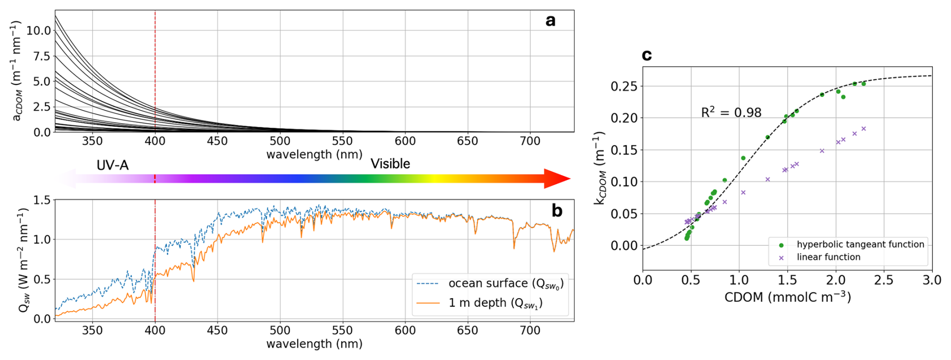
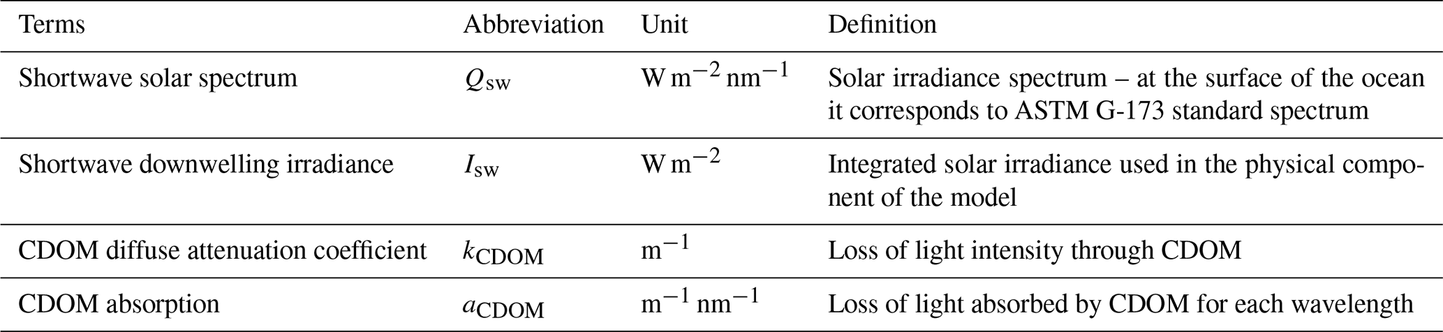
Figure 2 (a) In-situ CDOM spectral absorption measured over the Mackenzie Shelf during the 2009 Malina cruise for 31 water samples. (b) Shortwave solar spectrum (Q_sw) at the ocean surface ($Q_{{\mathrm{sw}}_{\mathrm{0}}}$; dashed blue line) and at 1 m depth after CDOM absorption ($Q_{{\mathrm{sw}}_{\mathrm{1}}}$; solid orange line). (c) CDOM attenuation (k_CDOM) relationship as it is described in Pefanis et al. (2020) (purple crosses) and in this study (green dots). The vertical red dashed line indicate the limit between UV-A and visible wavelength. Note that in Eq. (1) we are computing the shortwave radiation absorbed from surface ocean to 1 m depth ($Q_{{\mathrm{sw}}_{\mathrm{1}}}$), which results in the units being in W m⁻³ and hence k_CDOM having units of inverse meters.

In our ED-SBS configuration, we approximated the relationship between CDOM light attenuation and its mass concentration (mmol C m⁻³) in high CDOM environments such as Arctic river-influenced waters. In this regard, we empirically estimated the CDOM diffuse attenuation coefficient (k_CDOM; m⁻¹) from 31 in-situ measurements of the CDOM spectral absorption (a_CDOM[λ]; m⁻¹ nm⁻¹) across the SBS (Fig. 2a). The standard solar irradiance spectrum (ASTM G-173; U.S. D.O.E., 2005) was used as the reference shortwave solar spectrum at the surface ocean ($Q_{{\mathrm{sw}}_{\mathrm{0}}}$; W m⁻² nm⁻¹) – terms are listed in Table A1. We first calculated the shortwave spectrum attenuated from the surface ocean to 1 m depth ($Q_{{\mathrm{sw}}_{\mathrm{1}}}$; W m⁻³ nm⁻¹) by multiplying $Q_{{\mathrm{sw}}_{\mathrm{0}}}$ with a_CDOM[λ] (Fig. 2b). Then, k_CDOM was retrieved by integrating $Q_{{\mathrm{sw}}_{\mathrm{0}}}$ and $Q_{{\mathrm{sw}}_{\mathrm{1}}}$ over the chosen wavelengths for each station using Eq. (1).

$$\begin{array}{}\text{(1)}& k_{\mathrm{CDOM}}=\mathrm{1}-{\displaystyle \frac{{\int }_{\mathit{\lambda }}{Q}_{{\mathrm{sw}}_{\mathrm{1}}}\mathrm{d}\mathit{\lambda }}{{\int }_{\mathit{\lambda }}{Q}_{{\mathrm{sw}}_{\mathrm{0}}}\mathrm{d}\mathit{\lambda }}},\end{array}$$

where lambda is the discrete wavelength (nm). Then, CDOM concentrations were estimated from a_CDOM[440 nm] (m⁻¹) using the relationship from Neumann et al. (2020) (Eq. 2).

$$\begin{array}{}\text{(2)}& \mathrm{CDOM}={\displaystyle \frac{a_{\mathrm{CDOM}}\left[\mathrm{440}\mathrm{nm}\right]+\mathrm{0.2409}}{\mathrm{Mc}\times \mathrm{0.0478}}},\end{array}$$

where Mc is the carbon atomic mass (Mc = 12.0107 g mol⁻¹). Finally, we fitted a hyperbolic tangent function (Eq. 3) to obtain the relationship linking k_CDOM and CDOM concentrations across the range of conditions found in the SBS (Fig. 2c).

$$\begin{array}{}\text{(3)}& k_{\mathrm{CDOM}}=a\times \tanh (b\times \text{CDOM}+c)+d.\end{array}$$

As shortwave radiation and PAR were simulated independently in the physical and biogeochemical components of the model, we calculated two different sets of parameters for the $k_{\mathrm{CDOM}}/$CDOM concentration relationship for both components. Both relationships yielded R² ≥ 0.98. Parameters fitted with the full shortwave spectrum (used in the physical component) were: $a=-\mathrm{0.15}$, $b=-\mathrm{1.31}$, c=1.04, and d=0.12. Parameters fitted with PAR (used in the biogeochemical component) were: $a=-\mathrm{0.14}$, $b=-\mathrm{1.18}$, c=1.04, and d=0.10.

2.3 CDOM biophysical feedback

We included the effect of CDOM on light attenuation in the biogeochemical component of the model (which already included light attenuation by water and Chl a). PAR intensity (I(z), W m⁻²) at depth z is calculated according to the following equation:

$$\begin{array}{}\text{(4)}& \begin{array}{rl}I\left(z\right)& =(\mathrm{1}-f_{\mathrm{ice}})\times \mathrm{0.4}\times I_{\mathrm{sw}}\\ & \times e^{-[k_{\mathrm{w}}+k_{\text{Chl }a}\times \text{Chl }a(z)+k_{\mathrm{CDOM}}(z\left)\right]\mathrm{d}z},\end{array}\end{array}$$

where I_sw (W m⁻²) is the shortwave downwelling irradiance (input from the physical component of the model), for which 40 % is considered as PAR, f_ice is the ice-cover fraction, k_w is the diffuse attenuation coefficient for pure seawater (k_w = 0.04 m⁻¹), k_Chl a is the Chl a diffuse attenuation coefficient (k_Chl a = 0.04 m² mg Chl a⁻¹), Chl a(z) (mg Chl a m⁻³) is the total concentration in Chl a at depth z, and k_CDOM is the diffuse attenuation coefficient for CDOM at depth z.

We included the biophysical feedback of CDOM light attenuation ocean warming by including k_CDOM, integrated over the entire shortwave spectra in the physical component of the model (see Sect. 2.2). The physical component of the model already included the thermal effect of light attenuation by seawater, calculating a downwelling light decay profile (dk_sw; 1-D) based on Jerlov water types (Paulson and Simpson, 1977) and decreasing from the ocean surface to seafloor starting with a value of 1 at the surface. We included the thermal effect of CDOM light attenuation by calculating a CDOM light decay profile (dk_CDOM) based on k_CDOM (Eq. 5), also decreasing with depth starting from 1 at the surface. As CDOM concentrations are variable in space, the resulting light decay profile produces a 3-D field.

$$\begin{array}{}\text{(5)}& \left\{\begin{array}{l}\mathrm{d}{k}_{\mathrm{CDOM}}\left(\mathrm{0}\right)=\mathrm{1}\\ \mathrm{d}{k}_{\mathrm{CDOM}}\left(z\right)=\mathrm{d}{k}_{\mathrm{CDOM}}(z-\mathrm{1})\times e^{-k_{\mathrm{CDOM}}d(z-\mathrm{1})},\end{array}\right.\end{array}$$

where dk_CDOM(0), the decay at the surface ocean (0 m depth) is set to 1, since simulated light has not yet been affected CDOM and z−1 is the depth of the vertical grid cell above z. The dk_CDOM calculation is then propagated from the ocean surface to the seafloor, as its value at depth z depends on all the values above. We then multiplied both decay profiles to yield the total decay profiles (dk_tot; 3-D) as follows:

$$\begin{array}{}\text{(6)}& \mathrm{d}{k}_{\mathrm{tot}}\left(z\right)=\mathrm{d}{k}_{\mathrm{sw}}\left(z\right)\times \mathrm{d}{k}_{\mathrm{CDOM}}\left(z\right).\end{array}$$

The setup described above represents a significant advancement over the previous model development by Pefanis et al. (2020). We took the advantage of an extensive in-situ carbon dataset collected in 2009 to update the parameterization of CDOM mass fluxes as they transition between short and long-residence-time carbon loops, where it was previously represented using a single DOC pool (Dutkiewicz et al., 2015). We also revisited the $k_{\mathrm{CDOM}}/$CDOM relationship, transitioning from a linear to a hyperbolic tangent relationship (see Fig. 2c) This is particularly relevant for river plume regions where CDOM concentration reaches high values. Finally, our developments included the heating contribution of CDOM UV-A absorption, which contributes to roughly 40 % of CDOM light absorption in the Mackenzie shelf region. The ED-SBS setup presented here is thus able to better represent the terrestrial browning effect on Arctic coastal regions.

3 Results

The simulations presented herein include all model improvements detailed above (Run_full), i.e., a CDOM tracer communicating with two DOC pools, CDOM light attenuation as a hyperbolic tangent function, including UV-A attenuation heating effect, and riverine input (see Table 1). For the remainder of the study, we focus our analysis on the year 2012 – different from parameterization year (2009) – for two reasons: (1) sea ice area showed a major reduction during this year (Parkinson and Comiso, 2013) and (2) previous results by Pefanis et al. (2020) focus on this specific year. However, all simulations were performed with the same forcings over 5 years (2008–2012) to mitigate spin-up effects in processes directly affected by the inclusion of CDOM, such as dissolved carbon (DOC and DIC) concentration, or indirectly affected such as nutrient stock through changes in primary production. We also limit our analysis to the Mackenzie River plume region, which we define by the time-mean sea-surface salinity (SSS) isohaline of 27 (Fig. S1).

We also compute metrics that describe sea ice phenology, as defined in Bliss et al. (2019); these metrics are then spatially averaged over the plume region. The day of opening (DofO) and the day of closing (DofC) are respectively the first and last days when sea ice concentration is below 80 %. The day of retreat (DofR) and the day of advance (DofA) are respectively the first and last days when sea ice concentration is below 15 %. The period between these two days is the inner ice-free period (IIFP) or open-water period. The period between DofO and DofR is defined as the seasonal loss of ice period (SLIP) and the period between DofA and DofC is the seasonal gain of ice period (SGIP). The above metrics are summarized in a schematic (see Appendix C) and are also indicated on the top of the following figures.

3.1 Mackenzie River plume seasonal phenology

We first describe the seasonal phenology of several important physical and biogeochemical variables in the simulated Mackenzie River plume. In the river plume, Run_full simulates an average surface CDOM concentration of 0.85 ± 0.08 mmol C m⁻³ from August to May, with a peak of 2.04 mmol C m⁻³ during the spring freshet, followed by declining concentrations in July (Fig. 3, black line). With regard to the sea ice phenology in the river plume, the model simulates an open-water period of ∼ 4 months (115 d), with SLIP and SGIP lasting 1 month (13 June to 9 July) and 1 week (2 to 10 November), respectively. From January to June, the SST is on average near the seawater freezing temperature (−1.93 °C) and slowly starts heating up in June with increasing shortwave downwelling irradiance at the ocean surface ($I_{{\mathrm{sw}}_{\mathrm{0}}}$; Fig. 3b) and accelerating freshwater discharge. In July, ocean-surface shortwave downwelling irradiance reaches a maximum, rapidly heating SST until it reaches a peak value of 10.3 °C on 8 August. Then, temperatures slowly cool until the end of SGIP. Phytoplankton rapidly bloom during the SLIP period, with a peak in surface NPP of 8.35 Gg C d⁻¹ occurring two days after DofR. The production period – defined as the duration when NPP exceeds half of its maximum – lasts 7 d (7 to 14 July) and coincides with the period when subsurface light is the most intense. Nitrate and phosphate are quickly consumed during the phytoplankton bloom until the nitrate stock is depleted. Nutrient stocks are replenished through vertical mixing, advective transport, and remineralization from October to June. The simulated silicate tracer is directly connected to DSi riverine mass flux and therefore increases with elevated runoff.

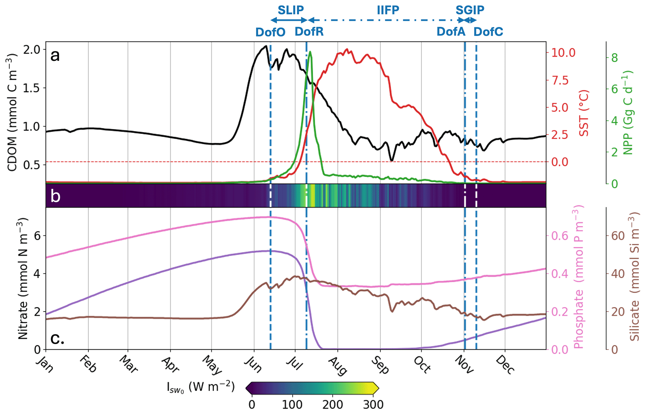
Figure 3 Spatially-averaged surface-ocean parameters simulated by Run_full in the Mackenzie River plume during 2012. Parameters shown are: (a) CDOM concentration (mmol C m⁻³; black line), SST (°C; red line), NPP (Gg C d⁻¹; green line), (b) shortwave downwelling irradiance at the ocean surface (I_sw0; W m⁻²), (c) nitrate concentration (mmol N m⁻³; purple line), phosphate concentration (mmol P m⁻³; pink line) and, silicate concentration (mmol Si m⁻³; brown line). The vertical dashed blue lines show the spatial-mean day of opening (DofO) and day of closing (DofC) and the vertical dashed-dotted blue lines show the spatial-mean day of retreat (DofR) and day of advance (DofA). Sea ice melting periods are shown consecutively, the seasonal loss of ice period (SLIP), the inner ice-free period (IIFP), and the seasonal gain of ice period (SGIP).

Within the Mackenzie River plume region, Run_full captures the mean SST amplitude and variability during the open-water period depicted by observations (Fig. D1). The model underestimates SST by 17 % from mid-July to mid-September. This is due to a later simulated SLIP, which delays surface-ocean heating and causes simulated SST to increase later in the season. Run_full also reasonably reproduces the amplitude of the phytoplankton bloom observed by remote sensing, as the simulated surface-ocean Chl a peaks at approximately the same concentration as reported by Lewis et al. (2020). However, the model underestimates the bloom's duration, simulating a bloom that lasts only half as long as observed by satellite. This discrepancy arises from the model's later simulated SLIP (similar to its SST behavior) and the rapid depletion of nitrates during the late open-water period. A more detailed and comprehensive model-data evaluation for 2012 is provided in Appendix D.

Table 1 Characteristics of the simulations tested in this study.

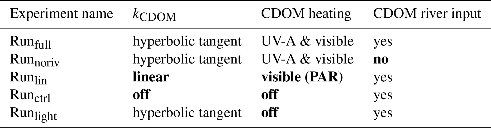
Changes to Run_full are highlighted in bold.

3.2 Adding riverine CDOM to ED-SBS

We next explore how the inclusion of riverine CDOM impacts light attenuation characteristics on the Mackenzie River shelf by comparing Run_full (presented above) to two similar set-ups: (1) excluding CDOM riverine forcing (Run_noriv; autochthonous CDOM only) and (2) using a linear CDOM light attenuation only in visible light (similar to Pefanis et al. (2020); Run_lin). We analyze the differences for the month of July, when shortwave downwelling irradiance (I_sw) is maximum and terrestrial CDOM is more likely to affect the biophysical characteristics of the plume region. The simulation excluding river mass flux exhibits a space-time mean k_CDOM of 0.02 m⁻¹ (Run_noriv) in the plume region (Figure 4a). Including riverine CDOM increases k_CDOM to 0.13 and 0.16 m⁻¹ when using a linear (Run_lin) and hyperbolic tangent (Run_full) relationship with CDOM, respectively. In the vicinity of the river mouth, k_CDOM reaches values 6.5 to 8 times higher than simulations without riverine CDOM forcing, highlighting the importance of including the riverine CDOM effect on light in the nearshore region. When using a linear relationship, k_CDOM increases as CDOM concentration increases, triggering high values (>0.3 m⁻¹ with a maximum at 0.59 m⁻¹) in the direct vicinity of the river mouth, with a sharp transition to lower values further offshore (<0.2 m⁻¹) (Fig. 4b). When using the hyperbolic tangent relationship, k_CDOM is capped to 0.26 m⁻¹, given the $k_{\mathrm{CDOM}}/$CDOM relationship fitted with in-situ observations (see Fig. 2c). As a result, CDOM attenuation is more evenly spread along the nearshore region (Fig. 4c).

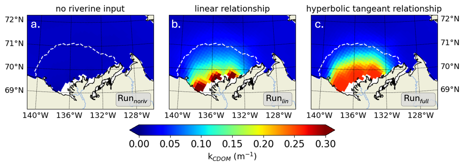
Figure 4 For July 2012, time-mean CDOM diffuse attenuation coefficient (k_CDOM, m⁻¹) for (a) Run_noriv, (b) Run_lin, and (c) Run_full. The white dashed line marks the time-mean spatial extent of the Mackenzie River plume.

3.3 Riverine CDOM biophysical feedback

We now examine how riverine CDOM influenced the physical conditions of the SBS during 2012, introducing a control simulation (Run_ctrl) that differs from Run_full by turning off both CDOM light attenuation (Sect. 2.2) and its effect on seawater heating (Sect. 2.3) (see Table 1).

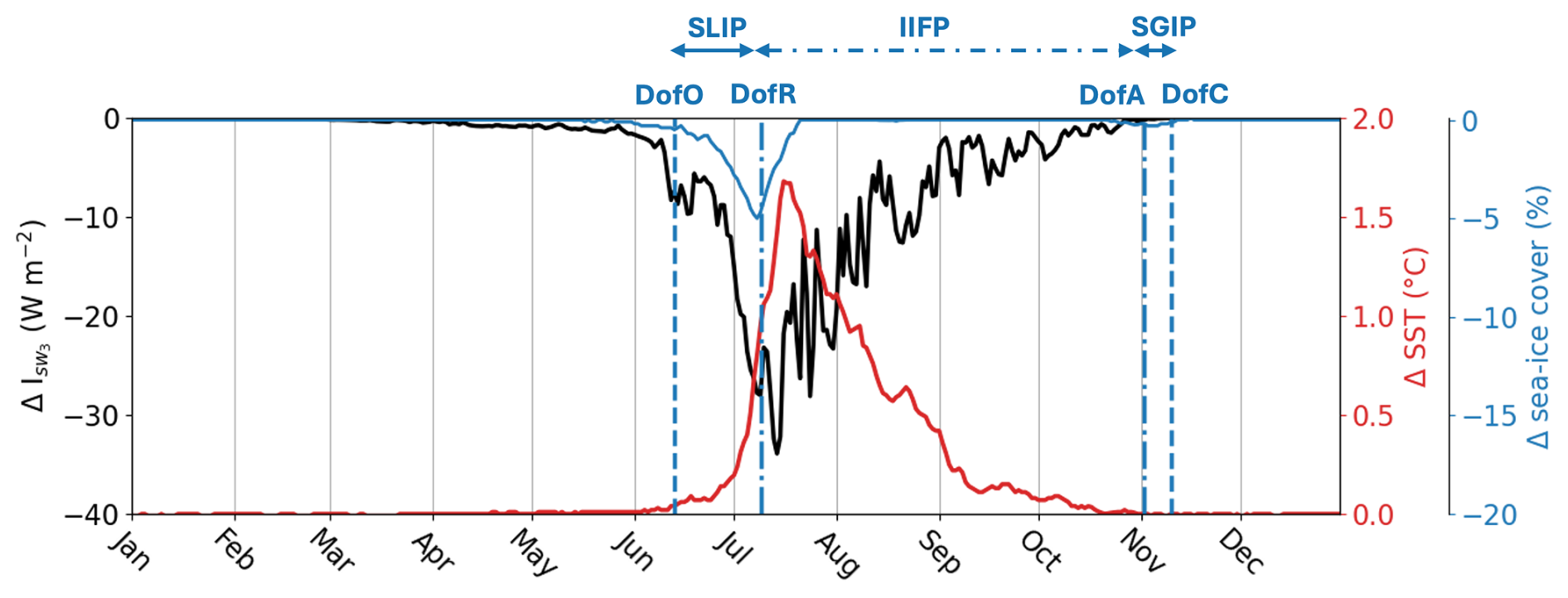
Figure 5 Difference in subsurface shortwave downwelling irradiance at 3 m depth ($I_{{\mathrm{sw}}_{\mathrm{3}}}$ in W m⁻²; black line), SST (°C; red line) and sea ice concentration (%; blue line) between Run_full and Run_ctrl. The vertical dashed blue lines show the spatial-mean Day of Opening (DofO) and Day of Closing (DofC) and the vertical dashed-dotted blue lines show the spatial-mean Day of Retreat (DofR) and Day of Advance (DofA) simulated by Run_full.

In the river plume, Run_full simulates a peak of surface CDOM concentration during the spring freshet, which coincides with the SLIP and the increase in surface-ocean shortwave downwelling irradiance (Fig. 3). As a result, the subsurface shortwave irradiance ($I_{{\mathrm{sw}}_{\mathrm{3}}}$) – defined as the shortwave irradiance (W m⁻²) below the model surface layer (3 m depth) – decreases by 13.4 W m⁻² (40 %) on average during the SLIP (Fig. 5) compared to the simulation without CDOM effects (Run_ctrl). CDOM light attenuation in the plume region then triggers an additional SST increase (ΔSST up to 1 °C), driving a decrease in sea ice cover by up to 5 % (Fig. 5). We note a delay of 1 d in the DofR in Run_full compared to Run_ctrl (not shown), demonstrating the limited influence of riverine CDOM on sea ice phenology. Terrestrial CDOM has a maximum impact on the physical condition of the plume one week after the DofR, with a 45 % decrease in subsurface shortwave downwelling irradiance and an increase of by up to 1.68 °C (Fig. 5). Finally, the impact of riverine CDOM gradually diminishes as the tracer becomes diluted in the open ocean during the IIFP.

Following the approach in Sect. 3.2, we analyze the influence of the k_CDOM parameterization on the river plume's temperature by comparing the changes in SST simulated by Run_noriv, Run_lin, and Run_full, relative to Run_ctrl. We focus on the month of July, when CDOM has the greatest impact on SST in the Mackenzie River plume (Fig. 6). In Run_noriv, the change in CDOM heating relative to Run_ctrl is solely attributed to marine CDOM produced by phytoplankton grazing and mortality. The spatially-averaged change in SST due to phytoplankton-generated CDOM, based on the improved CDOM-carbon loop connection (see section 2.1), is 0.45 ± 0.09 °C. The specific contribution of riverine CDOM leads to increases of 84 % (0.83 ± 0.24 °C, Run_lin) and 144 % (1.10 ± 0.28 °C, Run_full) using the linear and hyperbolic tangent $k_{\mathrm{CDOM}}/$CDOM relationships, respectively. We note that the k_CDOM relationship in Run_lin only considers a classic linear CDOM warming effect resulting from PAR attenuation, emphasizing the dominant role of UV-A in SST warming.

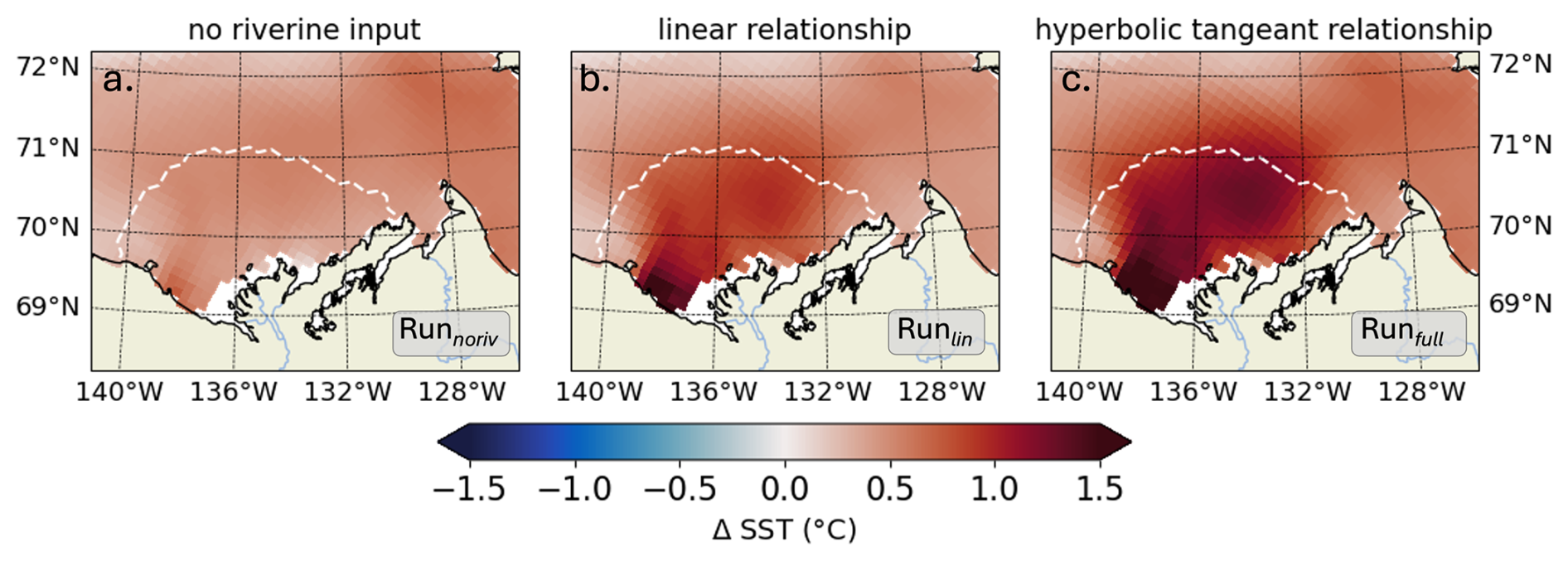
Figure 6 Time-mean SST differences (°C) for July 2012 between (a) Run_noriv, (b) Run_lin, and (c) Run_full, relative to the baseline simulation which excludes the CDOM effect (Run_ctrl). The white line in each panel indicates the mean extent of the Mackenzie River plume.

3.4 CDOM effect on marine primary production

In the remainder of the study, we explore the specific effects of CDOM light attenuation and ocean heating on the coastal primary producers and the carbon cycle, focusing on the biological and solubility pump. From here, we only focus on three simulations: Run_full, Run_light, and Run_ctrl. The later two simulations deviate from Run_full by turning off aspects of the CDOM light absorption (see Table 1): In Run_ctrl, we turn off both CDOM light attenuation (Sect. 2.2) and its effect on seawater heating (Sect. 2.3). In Run_light, we turn off only the CDOM heating effect (Sect. 2.3) but include its effect on light attenuation. We then disentangle the individual impacts of light attenuation and their influence on ocean temperature over seasonal timescales.

Annual surface-ocean NPP integrated in the river plume region remains similar across simulations, whether including the influence of CDOM on light and temperature (Run_full) or not (Run_ctrl), yielding 0.10 and 0.13 Tg C yr⁻¹, respectively. However, a mean delay of 15 ± 3 (min: 9–max: 23) days occurs in the seasonal phytoplankton bloom, defined here as the day when Chl a reaches its peak value. The surface-ocean NPP maximum, initially occurring in the middle of SLIP, is delayed to DofR by the end of the sea ice melt season due to CDOM (Fig. 7a). Introducing both CDOM light and biophysical parameterizations (Run_full) results in a 85 % increase in the peak of NPP, with 78 % attributed to the change in CDOM/light interactions and 7 % to increasing SST. However, the production period – defined as the duration when NPP exceeds half of its maximum – decreases from 12 to 5 d, thereby explaining the similar annual NPP.

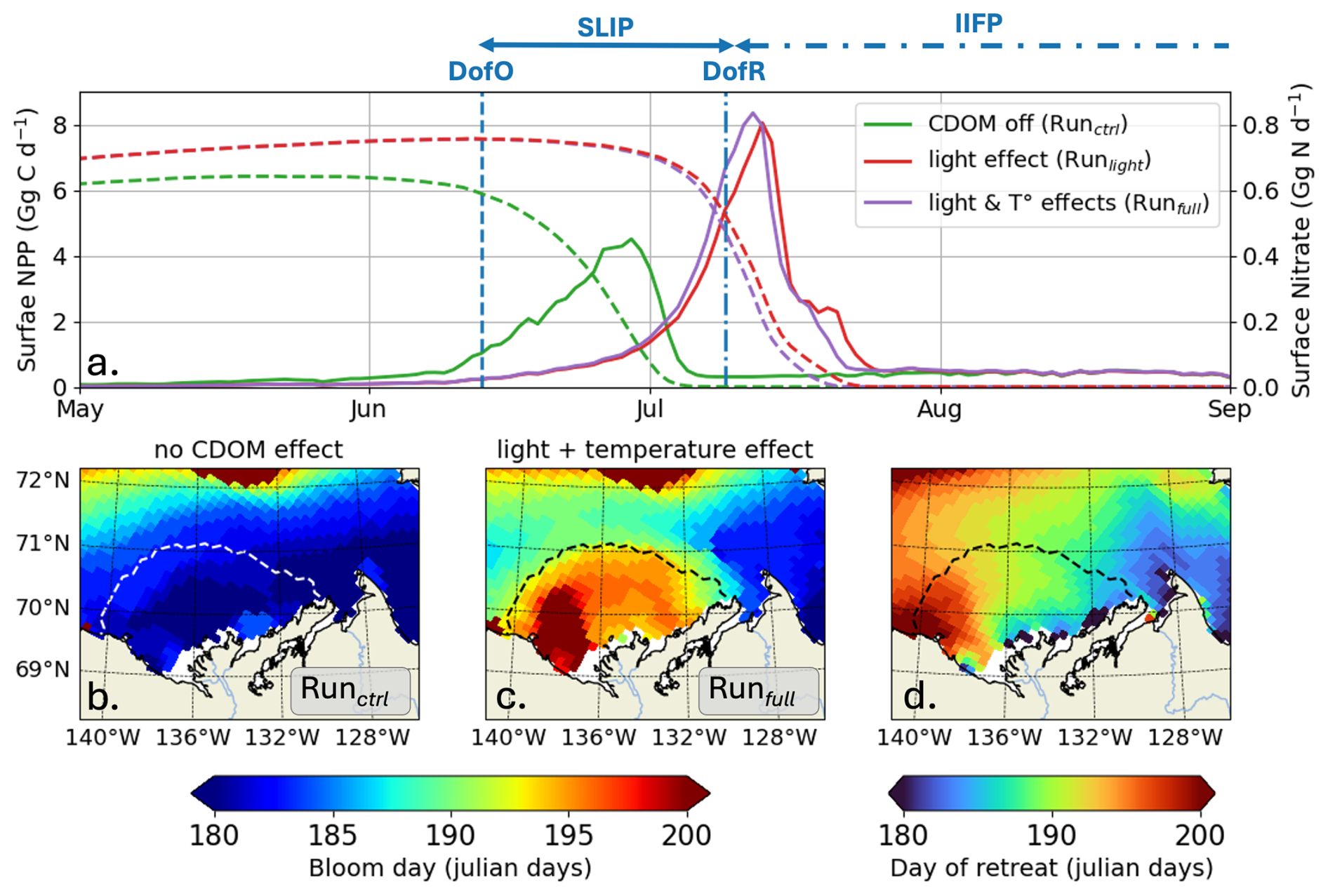
Figure 7 (a) Surface-ocean NPP (Gg G d⁻¹; thick lines) and nitrate stock (Gg N d⁻¹; dashed lines) simulated by ED-SBS without the CDOM light attenuation effect (green line; Run_ctrl), including (1) CDOM PAR light attenuation (red line; Run_light) and (2) CDOM light attenuation and ocean warming effect (purple line; Run_full). Maps of bloom day (julian days) (b) without the CDOM light attenuation effect, (c) including CDOM PAR light attenuation, and (d) map of DofR (julian days) simulated by EDS-SBS. Dashed line on the maps show the time-mean SSS isohaline of 27; vertical dashed and dashed-dotted blue lines show the DofO and DofR, respectively.

By early June, surface-ocean nutrient stocks are replenished through vertical mixing, advective transport, and remineralization that primarily occurred during winter – Note that the differences in May surface nitrate concentrations observed in Fig. 7a are related to changes in stock replenishment over the spin up period due to CDOM inclusion. High sea ice concentrations during most of the year result in light availability being primary limiting factor for phytoplankton growth, with temperature as a background limitation (See Appendix E). As the season progresses into SLIP the sea ice concentration decreases, leading to higher light penetration into upper-ocean waters. In Run_ctrl, this allows phytoplankton to utilize nutrients and initiates a bloom (Fig. S2a) that persists until the nitrate stock is entirely consumed and thus limits further phytoplankton growth. However, by early June, riverine CDOM (Run_light) drives additional light attenuation, counterbalancing the increased light penetration resulting from sea ice loss (see Fig. 5), hence slowing down the bloom initiation and delaying it by roughly 2 weeks (see Figs. 7 and S2b). Consequently, phytoplankton bloom latter in the season until the nitrate stock is exhausted and again limits further growth. We find an east-west gradient in the maximum bloom day (Fig. 7c), correlated with the DofR (Fig. 7d). This supports our hypothesis that light attenuation from riverine CDOM export complements light attenuation from sea ice during the melting period and delays the seasonal phytoplankton bloom until the open-water period.

3.5 CDOM effect on coastal air-sea CO₂ fluxes

In the absence of CDOM effects (light and heating effect), Run_ctrl results in a net annual CO₂ sink of −11.40 Gg C yr⁻¹ within the plume region. Over seasonal timescales, the air-sea CO₂ exchange occurs from DofO to DofC, with four distinct phases (Fig. 8). The following figures show the net air-sea CO₂ flux, integrated within the river plume region over the time period considered. The initial phase, starting from DofO and extending to one week after DofR, exhibits a substantial net CO₂ sink of −53.2 Gg C, which is attributed to phytoplankton growth (see Fig. 7). Following this, the second phase, which spans two months at the onset of the inner ice-free period (IIFP), is marked by a significant net CO₂ outgassing of 137.9 Gg C – this results from the decline in phytoplankton abundance and heightened local concentrations of DIC/DOC from river discharge (Bertin et al., 2023). Subsequently, a less-variable, one-month long phase follows, characterized by a delicate balance (air-sea CO₂ flux near 0 Gg C d⁻¹) that results in a moderate net uptake of −10.3 Gg C. The third phase, starting in early October and extending to one week after DofC, exhibits a strong net CO₂ sink of −99.2 Gg C. During this last phase, phytoplankton declines due to depleted nitrate levels and DIC/DOC concentrations return to background levels as river discharge diminishes.

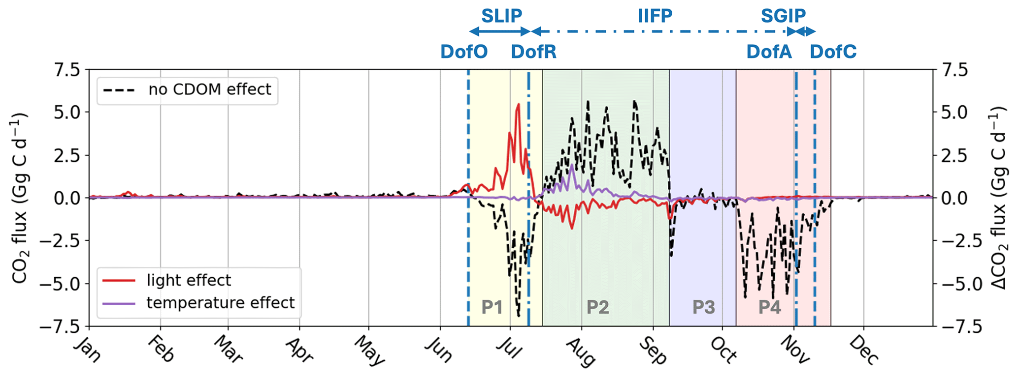
Figure 8 Air-sea CO₂ flux (Gg C d⁻¹) simulated by Run_ctrl in the plume region without CDOM biophysical feedback effects (black dashed line) and the change in air-sea CO₂ flux (Gg C d⁻¹) induced by the PAR light attenuation effect (red thick line) and warming effect (purple thick line). The vertical dashed blue lines show the average DofO and DofC and the vertical dashed-dotted blue lines show the average DofR and DofA. Phases with a switch in air-sea CO₂ flux simulated by Run_ctrl are indicated by four colors (P1: yellow, P2: green, P3: blue, and P4: red).

Over seasonal timescales, substantial changes in the timing and patterns of air-sea CO₂ flux occur during the two initial phases due to the inclusion of CDOM effects. As a result of CDOM light attenuation, we observe a delay in phytoplankton activity from the first phase (prior to DofR) to the subsequent phase (Fig. 7), leading to a 79 % reduction in simulated CO₂ uptake during phase 1 (+42.0 Gg C; Fig. 8). Furthermore, the increase in SST due to CDOM is minimal during this period (Fig. 5), resulting in a negligible impact on the net air-sea CO₂ flux (0.4 Gg C).

As the phytoplankton bloom simulated by Run_full peaks at the onset of the second phase, CDOM light attenuation reduces net CO₂ outgassing by 47.0 Gg C. However, the warming effect of SST counteracts the reduced CO₂ outgassing (caused by phytoplankton growth), driving a CO₂ outgassing of 19.8 Gg C during this period. Consequently, the net CO₂ outgassing for this period is reduced by 27.2 Gg C. Comparing the loss in CO₂ uptake on the first period (42.0 Gg C) and the gain in CO₂ uptake (−27.2 Gg C), the reduction in the CO₂ sink during the first period is 14.8 Gg C higher than the gain in the second period. Thus, changes in CO₂ fluxes during these two periods represent 80 % of the annual net loss in CO₂ sink. As a consequence, when including the CDOM bio-physical feedback (Run_full), the plume switches to a net annual CO₂ outgassing of 7.35 Gg C yr⁻¹. We show here that, despite the greater effect of light attenuation on the magnitude and sign of air-sea CO₂ flux, the temperature effect is the dominant contributor in the transition of the plume from a sink to a source of CO₂, as it dampens the increased CO₂ uptake due to phytoplankton growth in early summer.

4 Discussion

Assessing air-sea CO₂ fluxes in Arctic coastal environments remains challenging, as the carbon cycle and ecosystems are affected by a wide range of physical and biogeochemical processes that span the land-ocean continuum. As 11 % of the global river discharge is fluxed into the Arctic Ocean (McClelland et al., 2012), coastal waters are highly influenced by terrestrial browning (Lewis et al., 2020; Li et al., 2024), motivating the need to include this effect in ocean biogeochemistry models. In this study, we develop a new regional-scale ECCO-Darwin model that simulates (1) the impact of marine CDOM on the physical properties of the water column (Kim et al., 2018; Gnanadesikan et al., 2019; Pefanis et al., 2020) and (2) the interaction of terrestrial CDOM with the marine carbon cycle (Neumann et al., 2021; Clark et al., 2022).

Our model includes CDOM light attenuation (k_CDOM) as a hyperbolic tangent function of CDOM concentration, estimated from in-situ observations of CDOM spectral absorption from 280–750 nm on the Mackenzie Shelf. Using this relationship, simulated CDOM in the plume region compares reasonably well with both in-situ and satellite measurements (Matsuoka et al., 2012, 2017; Massicotte et al., 2021, see Appendix B). Furthermore, we show that using a hyperbolic tangent for k_CDOM limits the effect of CDOM light attenuation in high CDOM concentration regions, allowing for the light attenuation from CDOM to be distributed more evenly along the nearshore region (Fig. 4). Based on these results, we suggest that similar relationships be used in future models that aim to realistically represent coastal regions where CDOM concentrations reach high values (CDOM > 1.3 mmol C m⁻³ i.e., a_CDOM(440)>0.5 m⁻¹; Matsuoka et al., 2012). Additionally, this relationship was calculated from CDOM absorption integrated over the entire shortwave spectra, which includes the UV light absorption component, which is estimated to contribute up to 40 % of CDOM absorption on the Mackenzie Shelf. Therefore, our study considers the complete effect of CDOM attenuation on ocean heating, inducing a 36 % increase in the seasonal cycle of SST compared to previous methods (CDOM heating from PAR and k_CDOM as a linear relationship; see Run_lin and Gnanadesikan et al., 2019; Pefanis et al., 2020; Neumann et al., 2021).

Many ocean biogeochemistry models now incorporate land-to-ocean nutrient fluxes (Terhaar et al., 2019; Lacroix et al., 2021; Savelli et al., 2025), however, ocean circulation and physics often drive the biogeochemical state without the potential feedback of biogeochemistry on physics. In Arctic coastal regions, CDOM absorption has been reported to be a significant factor in the ocean heat budget (Hill, 2008; Soppa et al., 2019), but models still fail to include this feature. We find that including the CDOM heating effect in ED-SBS improved the model's ability to simulate the space-averaged SST observed during the early open-water season (Good et al., 2020, See Appendix D). We further show that riverine CDOM absorption contributes to a 1.7 °C increase in SST in the Mackenzie River plume, which is consistent with the increased seasonal amplitude previously reported for the AO (Gnanadesikan et al., 2019). The maximum increase occurs at the onset of the open-water season (0.2 °C d⁻¹), which is the same order of magnitude as observed in the Laptev Sea (Soppa et al., 2019). Although our model includes a component of CDOM generated by phytoplankton mortality and its associated light attenuation, we lack light attenuation by Chl a (Dutkiewicz et al., 2019), which has been shown to increase the SST signal by ∼ 0.5 °C along the Arctic continental shelves (Lengaigne et al., 2009). We note that the simulated increase in SST has a limited impact on sea ice, as we observe only a 5 % decrease in sea ice cover and a change in DOR by a single day.

By adding CDOM light attenuation to ED-SBS, we also observe a change in the simulated Mackenzie River plume phytoplankton bloom phenology. During the freshet season (early June), in Run_full, riverine CDOM triggers a small difference in light limitation (see Appendix E), which delays the phytoplankton bloom by two weeks to the end of the melting season. As a result of increased light penetrating the water column, the simulated phytoplankton bloom amplitude is 85 % higher and 1 week shorter due to rapid nitrate consumption. In the plume region, we further observe a westward gradient in the phytoplankton bloom peak day, which is correlated with the day of sea ice retreat (Fig. 7c and d). These results highlight that the coupling between CDOM and sea ice play a dominant role in shaping phytoplankton phenology, while the CDOM heating effect has a second order effect.

Further comparing simulated Chl a and primary production with satellite observations (Lewis et al., 2020) in the Mackenzie River plume (Note that these time-series are calculated where observations are available; more details in Appendix D), Run_ctrl and Run_full overestimate the average maximum in surface Chl a by 55 % and 62 %, respectively (Fig. 9a). However, Run_full better simulates the spatial distribution of surface Chl a especially in the vicinity of the coast (see Fig. D1). Run_full also successfully simulates the maximum in NPP observed by satellite (28 Gg C d⁻¹) while Run_ctrl underestimate it by 13 %. However, with respect to the initiation of the bloom Run_ctrl better matches observations (surface Chl a and NPP), where Run_full bloom initiates with a 2 to 3 weeks delay. Looking into more details on the sea ice melting behavior (SLIP equivalent with or without CDOM), we find that ED-SBS exhibits a shorter 2012 SLIP, with a 24 d delay in the DofO and a 16 d delay in the DofR. We therefore acknowledge that the combination of sea ice and CDOM light attenuation (Run_full) triggers the correct phenology in phytoplankton bloom initiation with respect to sea ice melting, but the incorrect timing as the bloom initiates 3 weeks later due to delayed DofO. This behavior in relation to the sea ice is confirmed in the comparison of averaged SST in the Mackenzie River plume (more details in Appendix D). As the observed melting season starts mid-May, SST rises in early June when DofR approaches, while simulated melting season only kicks in mid-June – 1 month after the observations – allowing a rise in SST by the beginning of July. Finally, the observed production remains high latter in the open-water season (August to September); ED-SBS is not able to sustain a high rate of primary production during this period as nitrate is entirely consumed, shutting down the bloom. The low simulated levels of Chl a after the bloom could be attributed to a match-mismatch with zooplankton.

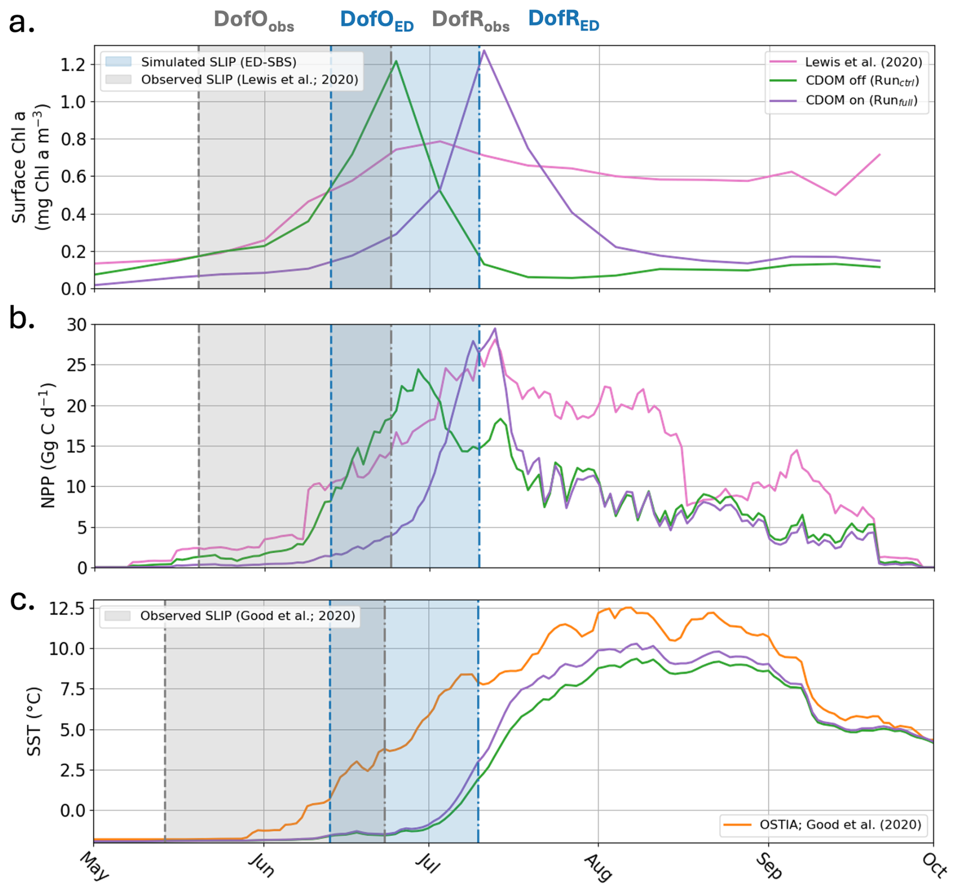
Figure 9 2012 (a) averaged Surface Chl a (mg Chl a m⁻³), (b) integrated NPP (Gg C d⁻¹), and (c) averaged SST (°C) over the Mackenzie River plume region for Run_ctrl (green line), Run_full (purple line), satellite observations (pink line; Lewis et al., 2020), and in-situ/satellite observations (orange line; Good et al., 2020). The blue (grey) area indicates the simulated (observed) seasonal loss of ice period.

We argue that including CDOM does not necessarily improve the phytoplankton phenology in the Mackenzie River plume compared to observations but does enhance its behavior regarding to sea ice melting. Furthermore, biophysical feedback of CDOM on water heating plays a non-negligible role in simulating SST in the region. We note that further improvements to the sea ice model and its interaction with phytoplankton would be required to accurately simulate the initiation of the bloom. The next version of ED-SBS, which will have high horizontal (∼ 1 km) and vertical resolution (∼ 1 m at the surface), will permit improved representation of fine-scale sea ice dynamics, such as cracks, leads, and specific features of the Mackenzie Delta such as the Stamukhi (Carmack and Macdonald, 2002; Matsuoka et al., 2016). Including melt ponds in future version of the model will also be necessary to improve the initiation of the phytoplankton bloom, as their impact on light penetration through sea ice has been reported to be important for the development of under-ice blooms (Ardyna and Arrigo, 2020; Clement Kinney et al., 2023). This might have an important effect as early snow melt and sea ice breakup are shown to enhance algal export in the Beaufort Sea (Nadaï et al., 2021). Finally, as a consequence of climate change and delayed sea ice freeze-up, Arctic phytoplankton phenology has been reported to transition to double bloom characteristics (Manizza et al., 2023), with a spring bloom initiated by under-ice blooms and low-light-adapted diatoms followed by an autumn bloom characterized by low-nitrogen adapted phytoplankton (Ardyna and Arrigo, 2020). The inclusion of the latter ecosystem components in ED-SBS could improve the phytoplankton representation in the latter open-water period, as our ecosystem is rapidly limited by nitrate concentrations. Furthermore, this hypothesis aligns with previous work by Choi et al. (2024), who showed that the inclusion of a nitrogen fixer (not dependent on nitrate) could explain the secondary fall bloom.

While the CDOM heating effect has a limited impact on phytoplankton phenology, its role in modulating air-sea CO₂ fluxes is crucial, especially for the annual budget. With the inclusion of CDOM light attenuation, and as a consequence of a two-weeks delay of the phytoplankton bloom, the strong CO₂ uptake that occurs during the melting period (without CDOM effect) disappears and shifts into a dampening of the early open-water period CO₂ outgassing (Fig. 8). Over annual timescales, this results in a decrease in the net CO₂ sink of 4.6 Gg C yr⁻¹, with the Mackenzie River plume region remaining a CO₂ sink. However, the inclusion of the CDOM heating effect and the 1.7 °C increase in SST at the onset of the open-water season promotes an increase in CO₂ outgassing due to reduced pCO₂ solubility, which balances the decrease in CO₂ outgassing driven by the phytoplankton bloom. Annually, CDOM heating promotes a 14.1 Gg C yr⁻¹ decrease in CO₂ uptake and switches the Mackenzie River plume region to a net CO₂ outgassing of 7.35 Gg C yr⁻¹. Although the contribution of the Mackenzie River to the Arctic CO₂ budget is small (Yasunaka et al., 2023), we demonstrate that CDOM is an important factor contributing to CO₂ fluxes in coastal regions. In the future, the projected increase in terrestrial organic matter fluxes may drive elevated CDOM levels in Arctic coastal regions, thus affecting the solubility pump and local marine ecosystems (Nguyen et al., 2022). This effect is likely to be even more important in the Eurasian Basin, where terrestrial CDOM export is more pronounced (Stedmon et al., 2011).

Our study focuses on the Mackenzie River plume region, which is the main contributor of particulate organic carbon (POC) at the pan-Arctic scale (McClelland et al., 2016). Similarly to CDOM, terrestrial POC fluxes are likely to increase in the future with increased runoff, permafrost thaw, and coastal erosion (Doxaran et al., 2015; Nielsen et al., 2024; Sauerland et al., 2025). The additional amount of carbon exported to the coastal waters by erosion alone could decrease the Arctic Ocean CO₂ uptake by 7 %–14 % by 2100 (Nielsen et al., 2024). Particulate organic matter also decreases the light available for primary production through absorption and backscattering (Stramski et al., 2004; Wozniak and Dera, 2007), potentially having an even stronger effect on the phenology. The effect of particle light backscattering may however overtake the effect of absorption, likely driving a decrease in coastal CO₂ uptake mainly by lower phytoplankton production rather than increased heat as shown with CDOM in this study. We acknowledge that ED-SBS does not account for terrestrial POC mass flux and the effect of suspended particulate matter on the attenuation of light (backscattering effect), which might be significant in this region (Lizotte et al., 2023). However, we focus here on the effect of the dissolved fraction and do not explore further assumptions regarding the particulate fraction effect, since our model does not account for solid sedimentation parameterization and bottom-sediment/seawater interactions. Future work will focus on the addition of a sediment model to fill this gap (Sulpis et al., 2022). Combined with the new Plankton, Aerosol, Cloud, ocean Ecosystem (PACE) satellite mission, which includes a hyperspectral imaging radiometer, the next generation of ED-SBS will be able to disentangle signature of Chl a, CDOM, and particulate matter to better estimate coastal Arctic CO₂ fluxes. Finally, the ECCO framework has paved the way for adjoint modeling at the global-ocean scale (Brix et al., 2015; Carroll et al., 2022). Future simulations will use adjoint modeling to optimize ED-SBS based on available physical and biogeochemical observations in the SBS.

5 Conclusions

We developed a new regional AO model which includes terrestrial CDOM export from the Mackenzie River. The CDOM component interacts with the marine dissolved carbon pool and its feedback on the physical properties of the water column, such as light intensity and temperature. In particular, ED-SBS simulates spectrally-resolved UV-light absorption, which has been thus far ignored in model studies and is estimated to contribute to 40 % of the light absorption in the SBS. We also suggest a new CDOM attenuation relationship as a hyperbolic tangent of CDOM concentration, which is able to better simulate light absorption in high CDOM concentration environments, such as river plumes.

In the plume region, we find that neglecting the coupled effects of light attenuation from sea ice cover and riverine CDOM export accelerates the timing of the simulated seasonal phytoplankton bloom by 2 weeks. Including riverine CDOM influence, the bloom occurs after the melting season, where light conditions are optimal, with a simulated phytoplankton bloom 85 % higher than simulations without effect of CDOM, but also 1 week shorter due to quicker consumption of nitrate. We further find that including the riverine CDOM biophysical feedback switches the net CO₂ sink in the plume region from −11.40 Gg C yr⁻¹ (without CDOM effects) to a net outgassing of 7.35 Gg C yr⁻¹. Although the change in phytoplankton phenology has a limited impact on the air-sea CO₂ fluxes, we find that the simulated outgassing is driven by the reduction in pCO₂ solubility resulting from a 1.7 °C increase in SST. Our modeling study demonstrates the importance of CDOM biophysical feedback in Arctic river plume regions, and the strong implications of CDOM radiative heating on pCO₂ solubility and air-sea CO₂ fluxes. Our results suggest that future climate change-induced increases in terrestrial organic matter exports could substantially affect ecosystems and air-sea CO₂ fluxes in shallow Arctic coastal regions where CDOM export is high.

Appendix A: List of terms

Table A1 List of terms used in this study.

Appendix B: Terrestrial CDOM ratio validation

We set the percentage of DOC_sr redistributed into the CDOM pool by performing a sensitivity experiment. Three different parameterizations of the riverine CDOM input were tested: Marine CDOM tracer is forced at the Mackenzie River mouth by (a) 1 %, (b) 2 %, and (c) 4 % of the total riverine tDOC mass flux. This percentage is subtracted from DOC_sr to CDOM as detailed in Sect. 2.1 (Fig. 1). Then, we compared the simulated light CDOM absorption (a_CDOM[λ]) derived from simulated CDOM concentration (see Eq. B1; Dutkiewicz et al., 2015) in the Mackenzie river plume, with in-situ observations of a_CDOM[440 nm] measured during the Malina campaign (see location of station in Fig. S1; Matsuoka et al., 2012; Massicotte et al., 2021) and remotely-sensed a_CDOM[443 nm] (Matsuoka et al., 2017).

$$\begin{array}{}\text{(B1)}& a_{\mathrm{CDOM}}\left[\mathit{\lambda }\right]=C_{\mathrm{CDOM}}\times e^{-S_{\mathrm{CDOM}}(\mathit{\lambda }-{\mathit{\lambda }}_{\mathrm{0}})}\times \mathrm{CDOM},\end{array}$$

where λ₀ is the reference waveband (λ₀ = 450 nm), C_CDOM is the CDOM absorption at λ₀ (C_CDOM = 0.18 m² mmolC⁻¹), and S_CDOM is the CDOM absorption spectral slope (S_CDOM = 0.018 m⁻¹).

We used 4 comparison metrics to compare retrieved CDOM absorption (a_CDOM[λ]) from simulated CDOM against observations: the median (± standard deviation), the correlation coefficient (r), the median percent error (MPE) and the unbiased root-mean-square error (URMSE). Additional information and equations for the comparison metrics are detailed in Sect. S3. We find that changing the percentage of tDOC forcing the CDOM pool has no impact on the correlation coefficient (Table B1). Size of discrepancies between the simulated and observed values (URMSE) are equivalent when riverine CDOM takes 1 % or 2 % of tDOC input but increases by 55 % to 117 % when forcing is set to 4 %. The MPE increases by 40 % to 89 % when doubling the tDOC exported to CDOM from 1 % to 2 % and increases from 84 % to 109 % when doubling the tDOC exported to CDOM from 2 % to 4 %. The median of a_CDOM[λ] is 0.08 ± 0.26 and 0.03 ± 0.25 m⁻¹ for in-situ and satellite observations, respectively. With 4 % and 2 % of tDOC forcing the CDOM pool, the simulated median of a_CDOM[λ] is respectively fourfold (and doubled compared to observations). The simulated median is closer to observations when forcing with 1 % of riverine tDOC. Comparing the time-mean 2009 CDOM absorption in the Mackenzie River plume region (Fig. B1), the model forced with 2 % of tDOC best fits the satellite data within the river plume area, while the model forced with 1 % of tDOC results in a consistent underestimate. According to metrics and the comparison of time-mean a_CDOM[λ] fields, parameterization 2 % (Table B1) was selected as the method best able to reproduce observed CDOM in the Mackenzie River plume region.

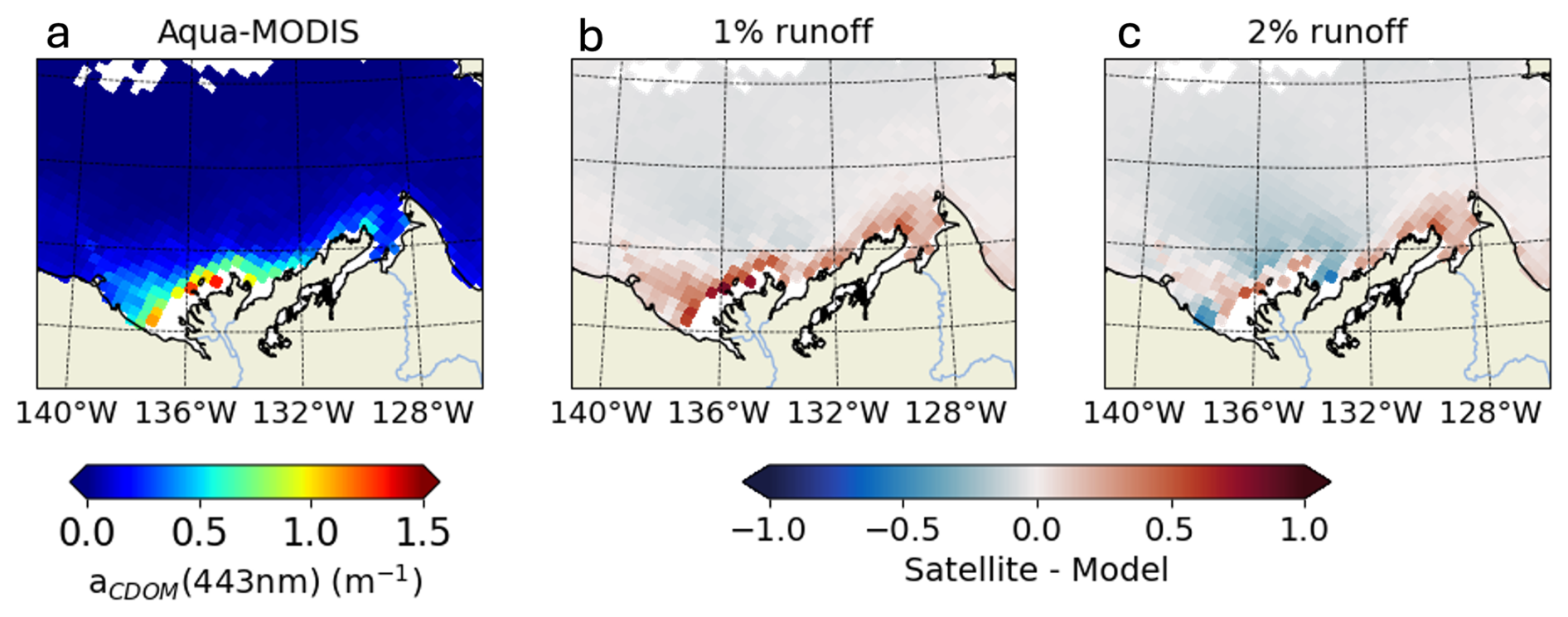
Figure B1 2009 annual-mean CDOM absorption at 443 nm from (a) remotely-sensed observations and differences from simulated CDOM fields with (b) 1 % and (c) 2 % of tDOC redistributed into CDOM tracer. Simulated CDOM absorption is compared with satellite observations that are space-time colocated with the simulations.

Table B1 Comparison metrics between simulated and observed a_CDOM[λ] (m⁻¹).

Appendix C: Sea ice phenology parameters

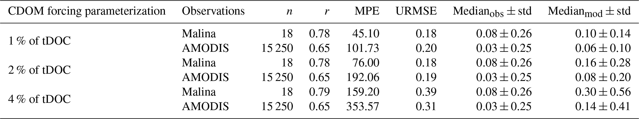
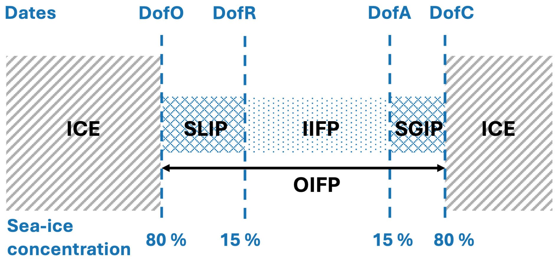
Figure C1 Conceptual diagram of sea ice seasonal evolution from spring/summer retreat (left) through fall/winter advance (right). Adapted from Bliss et al. (2019).

Appendix D: Comparison with observations

We compared the 2012 weekly surface-ocean Chl a (mg Chl a m⁻³) and daily primary production (mg C m⁻² d⁻¹) simulated by ED-SBS (Run_ctrl and Run_full) with satellite observations from Lewis et al. (2020) data estimated by the AOReg.emp algorithm. We also compared simulated daily-mean SST (°C) for 2012 in both models with in-situ/satellite observations (OSTIA; Good et al., 2020). As both observational products have a finer horizontal grid-spacing compared to ED-SBS, we bin-averaged the observations within each model grid cell. We then calculated the spatially-averaged value within the Mackenzie River plume region where satellite data were available to assess the model's ability to represent these observations (Figs. 9 and D1). Note that the number of observations (n) available within the river plume area ($n_{max}=\mathrm{281}$ for the entire area) varies in time. As both observational products provide sea ice concentration data, we also calculated observed sea ice phenology metrics to compare with our model simulations. Note that satellite observations from Lewis et al. (2020) AOReg.emp algorithm are the most suitable for model-observation comparison in the Mackenzie River plume, as they improve CDOM pollution removal in Chl a estimates, using different fits of the Chl $a/R_{\mathrm{RS}}$ (remote sensing reflectance) relationship for offshore region and shelf seas (where isobath <1000 m). However, the Beaufort Shelf being shorter than other Arctic Seas, the Mackenzie River plume spreads out further away from the shelf. We then observed an abrupt increase in Lewis et al. (2020) Chl a estimates along the shelf (1000 m isobath) due to the change in regional Chl $a/R_{\mathrm{RS}}$ fit (see Fig. S3) and decided to remove offshore data from the comparison. This only affected a small portion of the Northwestern plume region.

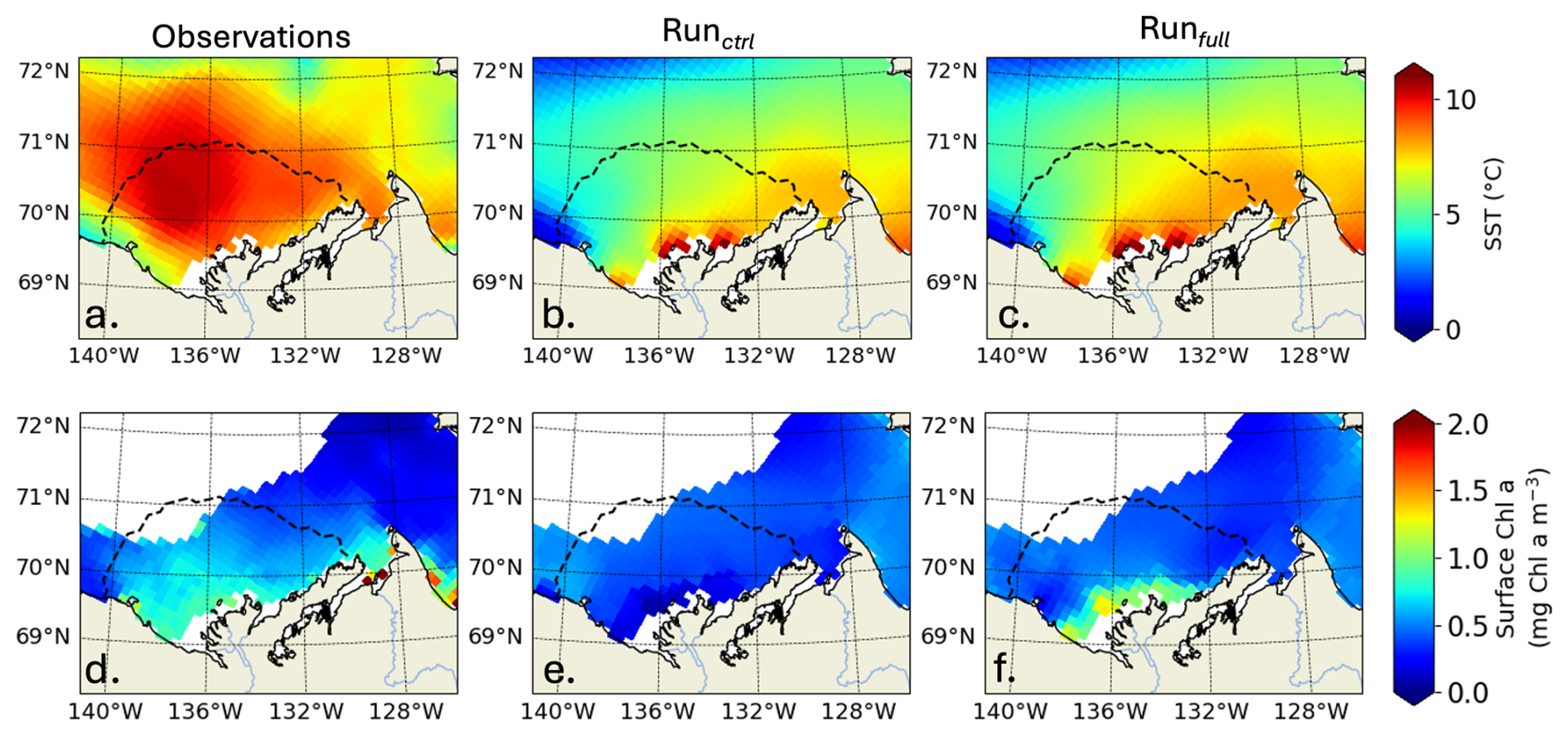
Figure D1 SST (°C) averaged from July to September 2012 (top row) and surface Chl a (mg Chl a m⁻³) averaged from June to July 2012 (lower row) for observations (a, d), Run_ctrl (c, e), Run_full (c, f). The dashed line shows the plume region (time-mean SSS isohaline of 27).

ED-SBS generally represents the spatially-averaged SST amplitude and variability in the Mackenzie River plume region during the open-water period compared to observations (Fig. 9c). The model underestimates SST by 25 % from mid-July to mid-September when CDOM is not included (Run_ctrl). Adding CDOM effects improves simulated SST by decreasing this underestimate to 17 % over the same period. However, similar to phytoplankton, we observe a delay in the surface-ocean heating, which is linked to later simulated SLIP. In the observations, SST starts increasing halfway through the melting season (Fig. 9c, orange line and grey area). In both simulations, SST also increases halfway through the melting season (Fig. 9c, purple and grey lines and blue area), but the SLIP occurs later in the season and thus surface-ocean warming also occurs later. We observe that this difference in June SST warming manifests mainly in the northwestern section of the plume where observed sea ice melting occurs first (not shown). Simulated sea ice first melts in the eastern section of the plume and propagates westward triggering a substantial difference in northwestern plume SST throughout the season compared to observations (Fig. D1a, b, c). However, the simulated eastern plume SST is comparable to observation improving by 13 % the correlation coefficient in the Mackenzie river plume. This confirms that sea ice plays an important role in the ability of ED-SBS to represent physics and biogeochemistry during the spring period.

Appendix E: Phytoplankton limitation factors

In ED-SBS, phytoplankton growth for each species (j) is limited by light, temperature, and nutrient availability. The three limitation factors (Eqs. E1, E2, and E3), which yield values between 0 and 1, are combined (multiplied) to provide the total phytoplankton limitation factor. In this study, we average both phytoplankton type limitation factors in the plume region (Fig. E1) to analyze the parameters affecting phytoplankton growth.

The factor with the lowest value is generally considered as the factor limiting phytoplankton growth. In the Arctic Ocean, as ocean temperatures are typically low, temperature is a consistent limitation factor year-round, shaping the background state of phytoplankton growth. In the SBS, the temperature limitation factor (γ^temp; dotted lines in Fig. E1) in the plume region ranges from 0.2 in winter to 0.4 during the open-water season. This seasonal change is mainly due to increased light penetration as a result of melting of sea ice and mixing of Mackenzie River-derived freshwater into the coastal ocean. The inclusion of CDOM heating has a limited influence on phytoplankton limitation. Therefore, in this study temperature limitation drives a consistent dampening effect in phytoplankton growth but does not influence phytoplankton phenology.

In winter, elevated sea ice cover causes high light limitation, with the spatially-averaged factor ranging between 0.4–0.6 in the plume region (Fig. E1). Additionally, nutrients concentrations are high (see Fig. 7), with a nutrient limitation factor over 0.8. Therefore, phytoplankton growth is limited by physics (both light and temperature). As sea ice begins to melt and break up (DofO), the light limitation factor increases up to to 0.8 – triggering the start of phytoplankton growth in both simulations. By early June, as riverine CDOM spreads in the plume region, a difference of 0.02 in the light limitation occurs between the simulations with (Run_full) and without (Run_ctrl) CDOM effects. This small difference is sufficient to trigger a slight difference in phytoplankton growth at this time, which allows the bloom to initiate in Run_ctrl (green dashed line; Fig. E1b) and thus delays the phytoplankton bloom by two weeks. In both simulations, elevated phytoplankton growth (mid-June or early July for Run_ctrl and Run_full, respectively) consumes nutrients, rapidly decreasing the nutrient limitation factor to ∼ 0 and stopping the phytoplankton bloom. Therefore, as the nutrient limitation factor exceeds the temperature limitation factor (on 3 July and 15 July without and with CDOM, respectively), the phytoplankton growth becomes primarily limited by nutrients. Analyzing each nutrient's (nitrate, phosphate, and silicate) limitation factor (not shown), we find that nitrate is the primarily limiting nutrient in the plume region.

In ED-SBS, the limitation factors for light (Eq. E1), temperature (Eq. E2), and nutrients (Eq. E3) are computed using the following equations:

$$\begin{array}{}\text{(E1)}& \left\{\begin{array}{l}{\mathit{\gamma }}_j^{\mathrm{light}}=\mathrm{1}-\text{exp}\left(\frac{{〈\mathit{\alpha }I〉}_j\text{Chl}a:C_j}{P_j^{\mathrm{Cm}}}\right)\text{if}{I}_{\mathrm{tot}}>I_{min}\\ {\mathit{\gamma }}_j^{\mathrm{light}}=\mathrm{0}\text{else},\end{array}\right.\end{array}$$

where I_tot and I_min are the total and minimum light intensity for phytoplankton growth (W m⁻²), respectively, α is the Chl a specific initial slope of the photosynthesis-light curve for each species, Chl a:C_j is the maximum Chl a to carbon ratio for each species, and $P_j^{\mathrm{Cm}}$ is the maximum growth rate.

$$\begin{array}{}\text{(E2)}& \begin{array}{rl}& {\mathit{\gamma }}_j^{\mathrm{temp}}\\ & =c^{\mathrm{Arr}}{\left[e^{A_{\mathrm{e}}^{\mathrm{Ar}}\left(\right(T+\mathrm{273.15})-T_{\mathrm{ref}}^{{\mathrm{Ar}}^{-\mathrm{1}}})e^{-e_{\mathrm{2}j}|T-T_j^{\mathrm{opt}}{|}^{p_j}}}\right]}_{\ge {\mathrm{10}}^{-\mathrm{10}}},\end{array}\end{array}$$

where T is the ocean temperature; c^Arr, $A_{\mathrm{e}}^{\mathrm{Ar}}$ and $T_{\mathrm{ref}}^{\mathrm{Ar}}$ the pseudo-Arrenhius equation coefficients set to 0.5882, −4000 K, and 293.15 K, respectively, and $T_j^{\mathrm{opt}}$ is the optimal phytoplankton temperature for each species.

The nutrient limitation factor takes the value of the most limiting factor between phosphorus, nitrogen, silicate and iron:

$$\begin{array}{}\text{(E3)}& \begin{array}{rl}& {\mathit{\gamma }}_j^{\mathrm{nut}}=min({\mathit{\gamma }}_j^P,{\mathit{\gamma }}_j^{\mathrm{N}},{\mathit{\gamma }}_j^{\mathrm{Si}},{\mathit{\gamma }}_j^{\mathrm{Fe}})\\ & \text{and}{\mathit{\gamma }}_j^{\mathrm{N}}=[{\mathit{\gamma }}_j^{{\mathrm{NO}}_{\mathrm{3}}}+{\mathit{\gamma }}_j^{{\mathrm{NO}}_{\mathrm{2}}}+{\mathit{\gamma }}_j^{{\mathrm{NH}}_{\mathrm{4}}}{]}_{\mathrm{0}}^{\mathrm{1}}\end{array}\end{array}$$

As nitrate is the primary limiting nutrient in this study, we describe below the nitrate limitation factor:

$$\begin{array}{}\text{(E4)}& {\mathit{\gamma }}_j^{{\mathrm{NO}}_{\mathrm{3}}}={\displaystyle \frac{{\mathrm{NO}}_{\mathrm{3}}}{{\mathrm{NO}}_{\mathrm{3}}+k_j^{{\mathrm{NO}}_{\mathrm{3}}}}}{e}^{-{\mathit{\sigma }}_j^{\mathrm{amm}}{\mathrm{NH}}_{\mathrm{4}}},\end{array}$$

where $k_j^{{\mathrm{NO}}_{\mathrm{3}}}$ is the half-saturation concentration for nitrate limitation and ${\mathit{\sigma }}_j^{\mathrm{amm}}{\mathrm{NH}}_{\mathrm{4}}$ is the coefficient for NH₄ inhibition of NO₃ uptake.

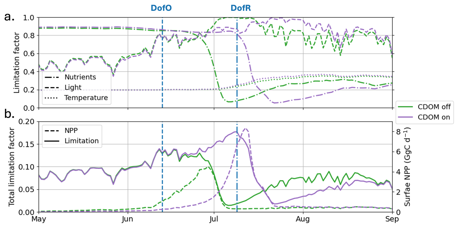
Figure E1 2012 (a) simulated limitation factors for nutrients (dash-dotted lines), light (dashed lines), and temperature (dotted lines), averaged between the two phytoplankton functional types and in the plume region for Run_ctrl (green lines) and Run_full (purple lines) and (b) simulated total limitation averaged between the two phytoplankton functional types and in the plume region and NPP spatially-integrated in the plume region for Run_full (purple lines) and Run_ctrl (green lines).