Aerodynamic flux–gradient measurements of ammonia over four spring seasons in grazed grassland: environmental drivers, methodological challenges and uncertainties

Understanding the factors controlling surface–atmosphere exchange of ammonia (NH₃) in grazed grasslands is crucial for improving atmospheric models and addressing environmental concerns associated with reactive nitrogen. This study presents high-resolution NH₃ flux data collected during four spring campaigns (2021–2024) at an intensively managed grassland site in Northwestern France, using the aerodynamic gradient method (AGM) alongside continuous monitoring of environmental variables and agricultural management. AGM-derived half-hourly NH₃ fluxes exhibited distinctive patterns: (i) high variability during grazing from −113 (deposition) to +3205 (emission) ng NH₃ m⁻² s⁻¹, influenced by meteorology, grazing livestock density, and vegetation and soil dynamics; (ii) strong diurnal patterns and day-to-day variability; and (iii) transient volatilisation peaks following slurry applications (up to 10 235 ng NH₃ m⁻² s⁻¹). Grazing-induced emission fluxes often persisted for up to 1–2 weeks following cattle departure. Relative random uncertainties associated with AGM flux measurements typically ranged from 15 % to 70 %, based on errors in vertical concentration gradient slopes and variables related to turbulence and stability. Additional methodological limitations and systematic uncertainties are discussed, in particular errors associated with fundamental AGM assumptions and flux footprint attribution in a rotational grazing setup. The mean overall cattle head-based emission factor (EF) was 6.5 g NH₃-N cow⁻¹ grazing d⁻¹ but varied considerably between grazing events, from 1 to 23 g NH₃-N cow⁻¹ grazing d⁻¹, reflecting the interplay between livestock management and environmental factors. This study highlights the importance of long-term, continuous, high-resolution measurements to document the large variability in grazing-induced NH₃ fluxes. The findings also underscore the need for refining bi-directional exchange models that integrate physics (meteorology, turbulence), environmental biogeochemistry (the fate of excreted nitrogen in the soil), biology (dynamic vegetation processes) and pasture management (grazing intensity) in grazed grassland systems.

1 Introduction

Agriculture is the largest global source of NH₃ emissions, accounting for 94 % of total emissions in the European Union, with livestock agriculture contributing 72 % (EEA, 2022). These emissions contribute to fine particulate matter (PM_2.5) formation, biodiversity loss, eutrophication and broader consequences for ecosystem health (Asman et al., 1998; Sutton et al., 2011). Additionally, dry-deposited NH₃ influences nitrogen cycling by promoting nitrification and denitrification processes that contribute to nitrous oxide (N₂O) emissions (Skiba et al., 2005), a potent greenhouse gas with ozone-depleting properties (Forster et al., 2021).

In grazed grasslands, NH₃ emissions originate primarily from nitrogen (N) in livestock excreta, deposited during grazing, and also from N applied as synthetic fertilisers and organic manures, such as cattle slurry, to sustain pasture growth. Urine, rich in urea, serves as the principal NH₃ source, with urease enzymes facilitating urea hydrolysis (Whitehead and Raistrick, 1993). Global NH₃ emissions from grazing are significant, though very uncertain, given the extensive grassland area, increasing livestock densities and excreta deposition on pastures (Sutton et al., 2022).

Ammonia volatilisation, i.e. the shift from aqueous-phase ammonium (NH${}_{\mathrm{4}}^{+}$) to gas-phase NH₃ and transfer to the atmosphere, is highly dynamic and influenced by environmental and management factors, including temperature, canopy structure, soil moisture and relative humidity, with emissions increasing under higher pH and warm conditions (Freney et al., 1983). The interactions between management practices, soil and meteorology create substantial temporal and spatial variability in NH₃ fluxes (Flechard et al., 2013; Sommer et al., 2003). Emission factors (EFs) represent the amount of nitrogen emitted per activity unit (e.g. the fraction of applied N, or the emission per cow per day) released as NH₃. Therefore, they exhibit significant variability depending on the same control factors. While EFs for fertilisation-induced NH₃ emissions are well-documented, grazing-related NH₃ fluxes remain poorly characterised due to scarce in situ micrometeorological measurement datasets. Most existing NH₃ EF estimates for grazing are often based on short-term studies, or artificial conditions, limiting their applicability for long-term assessments and modelling efforts (Bell et al., 2017; Sommer et al., 2019; Voglmeier et al., 2018).

Micrometeorological techniques such as the aerodynamic gradient method (AGM) and eddy covariance (EC) have been commonly used for field-scale NH₃ flux measurements. The AGM estimates fluxes based on vertical concentration gradients, turbulence measurements and Monin–Obukhov similarity theory, applying K-theory within the atmospheric surface layer (Monteith and Unsworth, 1990). It has been widely used in several ecosystems, including moorlands (Flechard and Fowler, 1998), crop fields (Loubet et al., 2012) and grasslands (Flechard et al., 2010; Milford et al., 2001; Wichink Kruit et al., 2007), often in combination with wet chemical instrumentation (e.g. Loubet et al., 2012), though optical systems are becoming more prevalent (Kamp et al., 2020, 2021). In contrast, EC provides more direct, high-temporal-resolution measurements of NH₃ fluxes using rapid-response (>5 Hz) analysers correlated with high-frequency wind velocity data (Famulari et al., 2005). However, both methods face similar challenges. The soluble, reactive and adhesive properties of NH₃ complicate concentration measurements, as adsorption and desorption on sampling surfaces (e.g. inlet tubing, filters) can introduce biases (Nemitz et al., 2004; Ellis et al., 2010; Schulte et al., 2024; Whitehead et al., 2008). Recent advancements in open-path analyser EC systems have mitigated these limitations for both AGM and EC (Swart et al., 2023).

A number of studies have demonstrated reasonable agreement between AGM and EC measurements, making them valuable tools for monitoring NH₃ flux dynamics (Swart et al., 2023) and other chemical species such as ozone (Loubet et al., 2013) and fumigants (Anderson et al., 2019). Alternative approaches, such as backward Lagrangian stochastic (bLS) modelling, have been shown to provide robust NH₃ emission estimates in controlled conditions by accounting for the geometry of the source (Häni et al., 2024).

The inherent complexity associated with micrometeorological methods necessitates extensive instrumentation and maintenance (Harper, 2005), thus increasing measurement costs and contributing to the scarcity of high-frequency, continuous NH₃ flux data and the large uncertainty in EF estimates (Sommer et al., 2019). Understanding the variability and drivers of grazing-induced NH₃ emissions under different conditions is crucial for improving process-based models, their eventual implementation in chemical transport models (CTMs) and EF estimates. Process-based models depend on accurate high-resolution measurements to improve surface–atmosphere NH₃ exchange parameterisations, which are essential for predicting atmospheric composition, improving air quality, assessing budgets and informing policies (Massad et al., 2020; Sutton et al., 2013).

In this study, we present multi-year, high-resolution NH₃ flux field-scaled measurements collected using the AGM with a closed path quantum cascade laser NH₃ analyser during four consecutive spring campaigns at an intensively grazed grassland monitoring site in NW France. To our knowledge, this dataset is one of the longest of its kind for NH₃ fluxes in pastures, which enables the investigation of NH₃ emissions over several grazing events, in contrasting weather and environmental conditions. Specifically, we aim to (i) quantify the temporal (diurnal, day-to-day, seasonal) dynamics of NH₃ fluxes associated with grazing activities, (ii) investigate the relationship between environmental factors and NH₃ fluxes, and (iii) evaluate uncertainties and methodological limitations of in situ AGM measurements in grazed grasslands.

2 Materials and methods

2.1 Site description

Ammonia flux measurements were conducted at the Integrated Carbon Observation System (ICOS) FR-Mej station (https://meta.icos-cp.eu/resources/stations/ES_FR-Mej, last access: 27 October 2025), located at the Mejusseaume dairy experimental research facility of the French National Research Institute of Agriculture, Food and Environment (INRAE, IEPL, 35650 Le Rheu, France; https://pegase.rennes.hub.inrae.fr/recherche/installation-experimentale, last access: 27 October 2025). The site, located about 10 km west of the city of Rennes, NW France, is situated at 48°7^′6^′′ N, 1°47^′48^′′ W with an altitude of 35 m above mean sea level. The soil is classified as a stagnic/luvic Cambisol with a sandy clay loam texture (20 % clay, 47 % silt and 33 % sand). The topsoil (0–30 cm) has a near-neutral pH (6.5, measured by 1 mol L⁻¹ KCl) with an average bulk density of 1.36 Mg m⁻³. The predominant wind direction during spring measurements in 2021–2024 was from the NW and SW directions; the main farm buildings are located to the SE (Fig. 1). The 4.7 ha field is managed as a pasture sown with ryegrass (Lolium perenne L.) with a transition to silage maize cropping for one season (May to September) every 5 to 6 years.

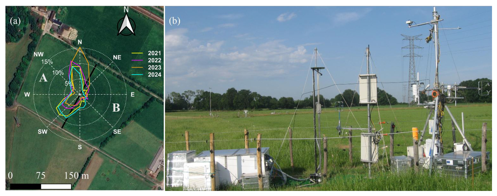
Figure 1 (a) Aerial view of the study area showing plot A (NW) and plot B (SE), with the fence shown as a black line and the wind rose indicating prevailing wind directions during the spring campaigns of 2021–2024 (© Google Maps 2025, mapped in QGIS software). (b) Field instrumentation setup, including the vertical NH₃ gradient profiling (mechanical lift) system, wind and turbulence sensors (3-D ultrasonic anemometers), and meteorological station.

This setup supports rotational grazing, with livestock grazing four to six times per year, including two to four phases concentrated in the spring when grass growth is vigorous. The dairy herd consists of the Holstein breed, which typically grazes 18–20 h each day, with feed supplementation provided during milking hours. The field is usually separated into two halves for grazing, i.e. NW (Plot A) and SE (Plot B) halves, each 2.35 ha. A fence running from NNE to SSW bisects the area, facilitating rotational grazing across the two plots (Fig. 1).

2.2 Measurement periods and management events

Flux measurements were conducted during spring campaigns from 2021 to 2024. Measurement periods varied across years, i.e. May–June in 2021, April–June in 2022 and 2023, and March–early July in 2024, capturing key management activities. Grazing did not occur simultaneously in both plots but rather in succession, requiring the two plots to be treated as distinct entities (Sect. 2.1). Stocking density varied from 16 to 55 livestock units (LSUs) per hectare across the 4 years. Fertilisation events with flux data coverage included two applications in 2022 (39 kg NH₄NO₃-N ha⁻¹ on 19 April and 53 kg N ha⁻¹ as cattle slurry on 31 May), one in 2023 (49 kg NH₄NO₃-N ha⁻¹ on 28 April) and one in 2024 (28 kg NH₄NO₃-N ha⁻¹ on 6 May). For this paper, we focus on 10 grazing events where data availability was reasonable to evaluate flux responses under grazing conditions. Details on stocking density, flux quality and data coverage for these events are summarised in Table 2.

2.3 Aerodynamic gradient method: theory and implementation

The surface–atmosphere NH₃ exchange fluxes were measured during spring grazing (June 2021–June 2024) using a modified hybrid version of the aerodynamic flux–gradient method (AGM) as described in Flechard and Fowler (1998). In contrast to the original full AGM described in earlier studies (Fowler and Duyzer, 1989), which uses profiles of wind speed and temperature, as well as gas concentration, a 3-D ultrasonic anemometer was used here to measure friction velocity (u_∗) and sensible heat flux (H) by eddy covariance.

2.3.1 Micrometeorology theory

The AGM relies on empirical relationships between turbulent fluxes and mean vertical gradients of NH₃ concentration (χ) above the surface (Monteith and Unsworth, 1990; Thom, 1975). This approach relies solely on measured vertical concentration profiles in situ on the field, with no measurement of the concentration profile upwind of the field. Following Fick's first law, and based on the Monin–Obukhov similarity theory, the turbulent NH₃ exchange flux between the surface and the atmosphere is described as the product of eddy diffusivity for heat and trace gases (K_H) and the vertical concentration gradient ($\mathrm{d}\mathit{\chi }/\mathrm{d}z$) measured in the inertial sublayer:

$$\begin{array}{}\text{(1)}& F_{\mathit{\chi }}=-K_{\mathrm{H}}{\displaystyle \frac{\mathrm{d}\mathit{\chi }}{\mathrm{d}z}},\end{array}$$

where z is the height above the ground. By convention, the negative sign implies that emission is positive and deposition is negative. The flux F_χ is assumed to be constant with height, under conditions of sufficient and homogeneous upwind fetch, stationarity ($\mathrm{d}\mathit{\chi }/\mathrm{d}t\sim \mathrm{0}$), negligible horizontal advection ($\mathrm{d}\mathit{\chi }/\mathrm{d}x\sim \mathrm{0}$), and negligible chemical sources and sinks in the air column below the maximum measurement height. However, both K_H and $\mathrm{d}\mathit{\chi }/\mathrm{d}z$ depend on height, limiting the practical implementation of Eq. (1). Sutton et al. (1993) demonstrated that Eq. (1) could be simplified as the product of two height-independent variables, i.e. friction velocity (u_∗) and a trace gas concentration-scaling parameter (χ_∗), such that

$$\begin{array}{}\text{(2)}& F_{\mathit{\chi }}=-u_{\ast }{\mathit{\chi }}_{\ast },\end{array}$$

with

$$\begin{array}{}\text{(3)}& {\mathit{\chi }}_{\ast }=-k{\displaystyle \frac{\mathrm{d}\mathit{\chi }}{\mathrm{d}\left[\ln \right(z-d)-{\mathit{\psi }}_{\mathrm{H}}\left(\frac{z-d}{L}\right)]}},\end{array}$$

where k is the von Kármán constant (0.41), d is the displacement height of vegetation or other roughness elements (calculated as $\mathrm{2}/\mathrm{3}\cdot$ canopy height), L is the Obukhov length and ψ_H is a height-integrated stability correction function, which accounts for the distortion effects of atmospheric stability or instability on the shape of scalar logarithmic profiles in the inertial sublayer (Panofsky, 1963; Paulson, 1970). In neutral and stable conditions, it is assumed that eddy diffusivities for momentum, heat and trace gases are equal; further, in stable conditions, ψ_H and the equivalent stability correction for momentum (ψ_M) are equal (Webb, 1970) such that

$$\begin{array}{}\text{(4)}& {\mathit{\psi }}_{\mathrm{H}}\left\{{\displaystyle \frac{z-d}{L}}\right\}={\mathit{\psi }}_{\mathrm{M}}\left\{{\displaystyle \frac{z-d}{L}}\right\}=-\mathrm{5.2}{\displaystyle \frac{z-d}{L}}.\end{array}$$

For unstable conditions, the height integration of the Dyer and Hicks (1970) similarity function for heat and trace gases was provided by Paulson (1970):

$$\begin{array}{}\text{(5)}& {\mathit{\psi }}_{\mathrm{H}}\left\{{\displaystyle \frac{z-d}{L}}\right\}=\mathrm{2}\ln \left({\displaystyle \frac{\mathrm{1}+x^{\mathrm{2}}}{\mathrm{2}}}\right),\end{array}$$

with

$$\begin{array}{}\text{(6)}& x={\left(\mathrm{1}-\mathrm{16}{\displaystyle \frac{z-d}{L}}\right)}^{\mathrm{1}/\mathrm{4}}.\end{array}$$

Micrometeorological data were collected to characterise turbulence and support NH₃ flux computations using Eqs. (2) and (3), based on instrumentation and software described in Table S1 in the Supplement.

2.3.2 Vertical profile concentration measurement system

The AGM was implemented using a gradient-lift ammonia sampling system (GLASS). The GLASS consisted of a concentration profiling setup with up to five measurement heights (0.1, 0.2, 0.5, 1.1 and 2.1 m) above the ground. A single heated, insulated 3 m long PFA inlet line ($\mathrm{1}/{\mathrm{2}}^{\prime \prime }$ o.d., $\mathrm{3}/{\mathrm{8}}^{\prime \prime }$ i.d) was sequentially and continuously lifted up, then lowered down, using a vertical mast with a winch and pulley, conveying the air sample to an NH₃ analyser (see Sect. 2.3.3). This single, vertically mobile inlet line with a large sampling flow rate was used to minimise potential concentration biases between different heights that may otherwise result from using several tubes associated with a set of solenoid valves. The lift system was custom-designed and built at the INRAE-IEPL workshop (Méjusseaume, Le Rheu, France) and was controlled by a CR6 datalogger (Campbell Scientific Inc, Logan, UT, USA), which was also used to perform all data acquisition and processing. The sampling procedure followed a 200 s sampling sequence from bottom to top, idling several tens of seconds at each of the three to five designated sampling heights for the concentration to stabilise, then moving on to the next height, with around 50 s of discarded integrated travelling time (unused for gradient determination) per 200 s cycle. An example half-hour time series is shown in Fig. S1 in the Supplement.

2.3.3 Air sampling and ammonia detection

The air sample was drawn into the ammonia analyser using an Edwards XDS35i dry scroll pump (Edwards Ltd, Burgess Hill, West Sussex, UK) placed downstream of the measurement cell. An auxiliary pump (KNF model N940, KNF Neuberger GmbH, Freiburg, Germany) with a flow rate of 25 slpm was attached to a T-junction connecting the main sampling line to the “sample IN” port of the analyser; this auxiliary pump increased the airflow up to 35 slpm in the inlet line (before the entry point into the analyser), helping reduce the residence time of the sample and signal attenuation associated with potential NH₃ adsorption to inner surfaces of the PFA tube.

The sampling head was fitted with a Teflon©-coated aluminium cyclone to remove coarse aerosols from the air sample (model URG-2000-30EHB, URG Corp, Chapel Hill, NC, USA), with a nominal 1 µm cut-off point for a 16.7 slpm sampling rate. The only filter in the NH₃ sampling system was a 47 mm diameter, 1.2 µm pore size PTFE filter located inside the analyser, which was required to preserve the very large mirror reflectivity inside the optical cavity. Ammonia concentrations were measured at 1 Hz resolution/integration time by a Los Gatos Research off-axis, integrated cavity output spectroscopy (OA-ICOS) quantum cascade laser (QCL) analyser (model LGR-FTAA, Fast Trace Ammonia Analyser, ABB/LGR group, San Jose, CA, USA). The nominal precision (1 SD) of the QCL analyser, provided by the manufacturer, was 0.2 ppb at a 1 s integration time and 0.08 ppb at a 10 s integration time; the instrument was similar, though not identical, to the model described by Leen et al. (2013). Notable differences in our analyser included a larger critical orifice (1.7 mm), a larger sampling rate through the cell (10 slpm) using a different pump and a lower cell pressure set point (100 Torr).

2.3.4 Gradient concentration data processing and corrections

When AGM flux measurements are conducted with a single concentration detector measuring non-simultaneously at two or more heights above the surface (sequential sampling), the vertical gradient may be biased (high or low) due to non-stationarity in the air mass if temporal concentration changes ($\mathrm{d}\mathit{\chi }/\mathrm{d}t$) are significant during the interval it takes to sample a full vertical profile (Fowler and Duyzer, 1989; Kamp et al., 2020). To minimise biases on the measured flux, we applied a linear concentration detrending procedure for individual height measurements based on the concentration change between two consecutive cycles of the lift sampling system (see Sect. S2 in the Supplement). Only the last 10 s of the concentrations measured during the 30–50 s of stabilisation time at each sampling height (before the sampling head moved to the next position) were used in the final concentration averaging (see Figs. S1 and S2 for a comparison with other averaging times and a sensitivity analysis for flux calculations). The stabilisation time was implemented to reduce memory effects from the previous height because NH₃ is known to stick to inner sampling surfaces (tubes, filters, cell) of closed path measurement systems. Step concentration change tests carried out both in the field and in the lab, fitted with a typical double exponential function versus time, indicated mean characteristic fast and slow time constants of 1.4 and 10 s, respectively (see Sect. S3), showing that the stabilisation times were long enough. Nine 200 s sampling cycles were performed, then averaged, within each half-hour (see Fig. S1), which was the time resolution for turbulence and flux calculation and averaging.

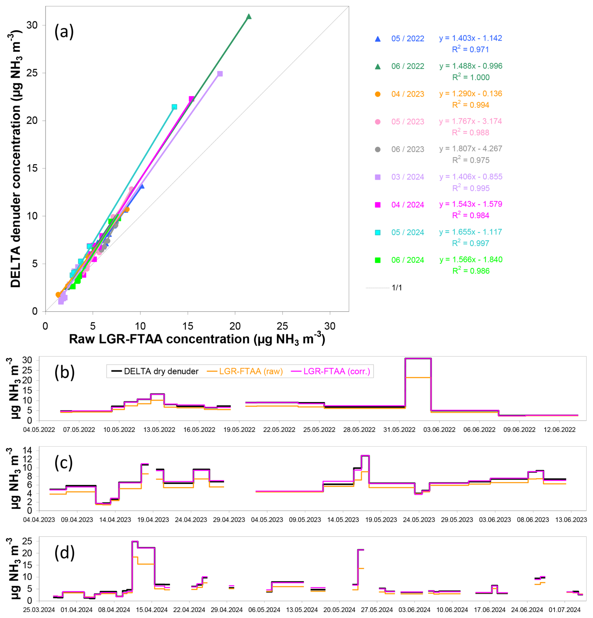
Figure 2 A posteriori correction procedure for LGR-FTAA QCL NH₃ concentrations using DELTA^® dry denuder concentrations as a reference. (a) Linear regression of time-integrated DELTA^® concentrations versus LGR-FTAA average raw concentrations calculated over each of the DELTA^® sampling intervals from 2022 to 2024 (co-located sampling at 1.1 m aboveground). (b–d) Time series of mean NH₃ concentrations for all DELTA^® sampling intervals, with raw LGR-FTAA QCL concentrations and corresponding values corrected based on the respective regression slopes and offsets from (a).

As no reliable gas-phase calibration system was available to check or calibrate the LGR-FTAA instrument in the ambient concentration range encountered in the field, at the large operating flow rates (see Sect. 2.3.3), we used an indirect, a posteriori correction method based on a comparison with another, co-located, absolute NH₃ sampling method (DELTA^® denuder system; see procedure described in detail in Sect. S1) placed within 1 m distance at the same height of the mast midpoint (1.1 m aboveground). A comparison of NH₃ measurements by both systems is shown in Fig. 2. This correction of the absolute concentration is necessary because a slope deviation from 1 affects the vertical gradient (and flux) proportionately and because accurate concentrations are required for compensation point or deposition velocity studies. AGM fluxes were then computed utilising Eq. (2) with the slope of the stability-corrected vertical concentration gradient (χ_∗) calculated by a linear least-square regression of χ versus the quantity ln$(z-d)-{\mathit{\psi }}_{\mathrm{H}}\mathit{\left\{}\right(z-d)/L\mathit{\}}$ (Eq. 3); by default, the flux calculations presented in the paper were made with concentrations measured from 0.5 m up to 2.1 m above the surface (see also discussion on flux uncertainty in Sects. 3.5 and 4.1.3). An example of the resulting half-hourly time series of the GLASS LGR-FTAA NH₃ concentration profile and calculated fluxes is shown in Fig. 3c–d.

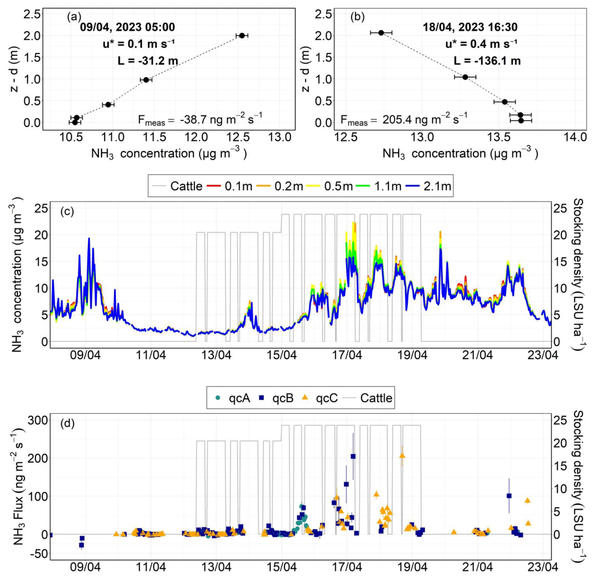
Figure 3 (a) Example of a vertical NH₃ concentration profile indicating dry deposition in background conditions (9 April 2023, 05:00 UTC+1). (b) Example of an NH₃ concentration profile during grazing (18 April 2023, 16:30 UTC+1), showing an emission event during windy neutral conditions. (c) Time series of NH₃ concentrations at different heights (0.1–2.1 m), illustrating the contrast between the pre-grazing and grazing periods. (d) Time series of NH₃ fluxes calculated by AGM over the same interval, where positive fluxes indicate emission and negative fluxes indicate deposition. The qcA, qcB and qcC symbols refer to best, good and modest quality fluxes (see Table 1). In panels (a) and (b), the given NH₃ error bar is equivalent to ±0.1 ppb (∼0.07 µg m⁻³), which is roughly the manufacturer's specification for a 10 s integration time; note this does not reflect the NH₃ variability (standard deviation) over the half-hour, which is much larger.

Table 1 Quality classification of validated NH₃ flux measurements based on micrometeorological screening (qc_μmet) and footprint contribution criteria. qcA: best quality flux; qcB: good quality flux; qcC: modest quality flux.

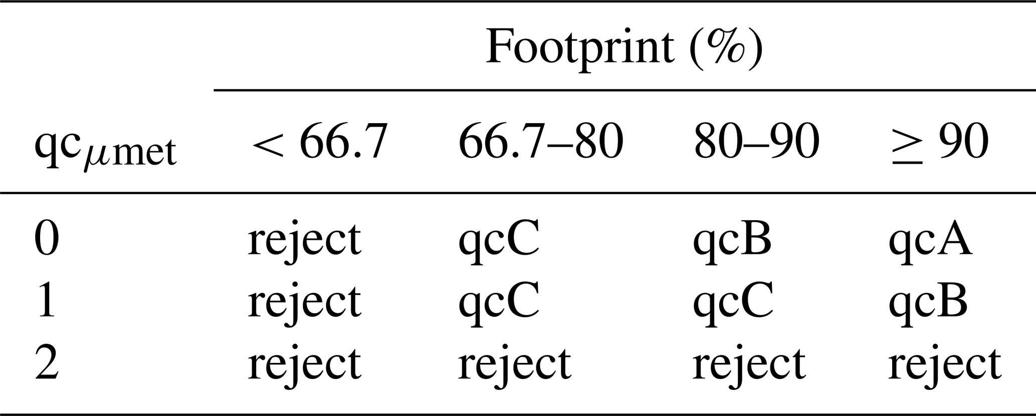
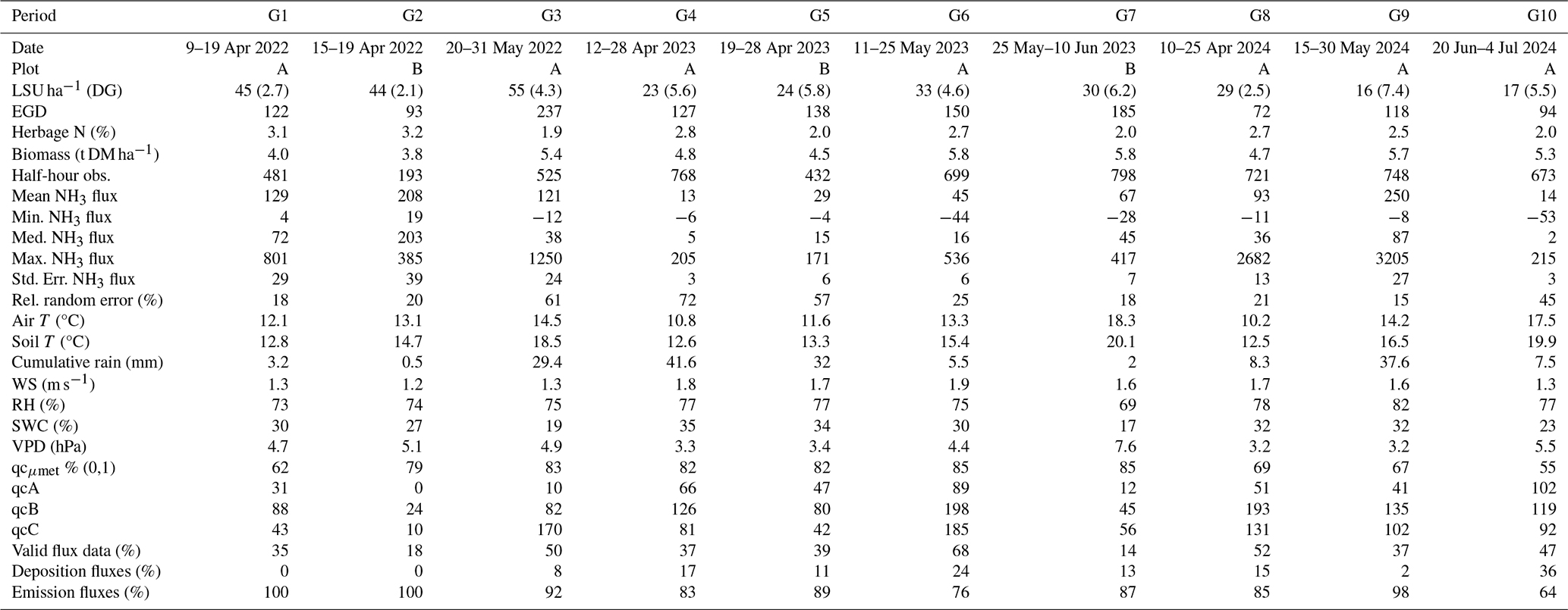
Table 2 Summary of management practices, environmental conditions, NH₃ fluxes and quality metrics across 10 grazing events (G1–G10). Data include NH₃ fluxes (ng NH₃ m⁻² s⁻¹), stocking density during the grazing interval (LSU ha⁻¹), grazing duration (DG), effective grazing days (EGD, defined as stocking density multiplied by grazing duration), grass nitrogen content, aboveground biomass measured before grazing started, and meteorological variables (average temperature, wind speed (WS), relative humidity (RH), soil water content (SWC) and vapour pressure deficit (VPD)). Flux data quantity and quality are represented by counts of half-hourly qcA, qcB and qcC flux values. The qc_μmet percentage indicates the proportion of valid half-hourly flux measurements meeting quality criteria (0 or 1). The percentage of final valid flux data equals % qc_μmet minus the additional fraction removed due to insufficient footprint contribution.

2.4 Flux data processing, corrections and quality control procedures

To ensure the integrity and quality of flux measurements, the following procedures were applied.

2.4.1 Storage flux correction

Temporal variations in NH₃ storage within the air column below the mean measurement height of the gradient system (z_mean=1.1 m) were considered. For NH₃, where exchange fluxes are significantly large compared to the concentration, the flux divergence attributed to storage change is typically considered negligible, as mentioned by Sutton and Fowler (1992). Nevertheless, the error in the flux due to storage (F_sto) was systematically calculated from the following equation, based on concentration changes from one half-hour to the next:

$$\begin{array}{}\text{(7)}& F_{\mathrm{sto}}=\underset{\mathrm{0}}{\overset{z_{\mathrm{mean}}}{\int }}{\displaystyle \frac{\partial \mathit{\chi }}{\partial t}}\mathrm{d}z.\end{array}$$

2.4.2 Footprint attribution

Because there was only one flux measurement setup on the field, differences in management practices between adjacent plots necessitated precise footprint attribution, especially under rotational grazing and frequent changes in wind direction. The Kormann and Meixner (2001) footprint model was employed to calculate the contributions of specific field areas to the measured fluxes, namely, from plot A, the primary footprint sector from SW through NW winds, and from plot B, fluxes under NE through SE wind directions (Fig. 1). For time intervals when plots A and B were under differential management, i.e. one plot was grazed or fertilised while the other was not, a minimum footprint contribution of $\mathrm{2}/\mathrm{3}$ (66.67 %) was required for the measured flux to be considered representative of the plot of interest. Fluxes for which footprint contributions from either plot were less than the $\mathrm{2}/\mathrm{3}$ threshold were discarded (for the plot of interest). If the $\mathrm{2}/\mathrm{3}$ footprint threshold was exceeded in one plot, the flux was validated and then corrected for the background interference from the fraction of footprint outside the plot of interest (see Sect. 2.4.5). For time intervals when plots A and B were under the same management (e.g. fertilisation of the whole field), both plots were assumed to have similar flux levels, and thus no footprint correction was applied.

2.4.3 Filtering of flux measurements

The flux data were further filtered to exclude flux measurements that did not meet steady-state, fully developed turbulent conditions and stationarity for momentum, sensible heat and trace gas fluxes.

1. Momentum and sensible heat flux screening: the 0–1–2 quality flagging system by Mauder and Foken (2004) was applied to EC fluxes of momentum (qc_τ) and sensible heat (qc_H) to ensure adequate quality of EC-derived friction velocity (u_∗) and sensible heat flux (H) for the purpose of AGM flux calculations (details provided in Sect. S4).

2. NH₃ stationarity: a qc${}_{{\mathrm{NH}}_{\mathrm{3}}\mathrm{stationarity}}$ quality flag was devised to assess the stationarity of NH₃ concentrations within each 30 min interval, based on the coefficient of variation (CV) of the nine NH₃ concentrations (averages of selected 10 s data) measured over the nine vertical lift ascents per half-hour. A flag of 2 was assigned to data where the maximum CV of all sampling heights exceeded 100 %, indicating high variability and non-stationary conditions, unsuitable for flux calculations. Data with CV values <10 % were flagged as 0, while values between 10 % and 100 % were flagged as 1 and retained.

3. Stability parameter: fluxes were filtered based on the stability parameter $\mathit{\zeta }=(z_{\mathrm{mean}}-d)/L$, where z_mean is the mean measurement height of the profile system (1.1 m). This filter excluded extreme stability conditions where the flux–gradient relationship deteriorates and stability corrections become less reliable. Data with ζ values outside predefined thresholds ($<-\mathrm{0.5}$ or >0.2) were flagged as 2 and excluded. Data within the range from −0.2 to 0.05 were flagged as 0 (best quality due to proximity to atmospheric neutral stability), while values between −0.5 and −0.2 (moderately unstable) or between 0.05 and 0.2 (moderately stable) were flagged as 1 and further retained.

4. Micrometeorological screening: the overall micrometeorological score qc_μmet was determined by combining the maximum flag scores of qc_τ, qc_H, qc_L and qc${}_{{\mathrm{NH}}_{\mathrm{3}}\mathrm{stationarity}}$. Half-hours with a score of 2 were excluded, and only measurements meeting all individual screening criteria (0 or 1) were retained for further flux analysis, ensuring high data quality for AGM flux computations.

2.4.4 Classification of flux quality

The fluxes were categorised according to the micrometeorological screening scores and footprint contribution, as shown in Table 1.

2.4.5 Corrections for background flux interference

During grazing on the plot of interest (whether A or B, depending on the date), corrections were applied to account for the potential “dilution” of the targeted emission fluxes by background fluxes from adjacent (ungrazed) plots in cases where there was an overlap in the measurement footprint. Because the threshold for footprint validation was $\mathrm{2}/\mathrm{3}$ for the plot of interest, up to $\mathrm{1}/\mathrm{3}$ of the flux footprint was potentially located in an adjacent plot, which we assumed to be in a state of background flux, i.e. a small or near-zero emission or deposition (see e.g. Flechard et al., 2010). The measured flux (F_meas) was therefore adjusted using a simple canopy compensation point model approach to estimate the background flux (F_bgd) (see Fig. S16) over adjacent fields, based on resistance modelling and environmental conditions (Massad et al., 2010; Nemitz et al., 2001). The grazed field fluxes (F_g) were adjusted following Eqs. (8)–(9) to ensure that flux values more accurately reflected true emission fluxes on the grazed field. Such corrections are tentative because the true background flux of the adjacent plot is not known and estimated using a modelling approach, but the absence of such correction would very likely result in underestimation of the actual emission by grazing.

In practice, we assumed that the net measured flux (F_meas) was composed of the two components F_g and F_bgd weighted by their respective percentage footprint contributions FP_g and FP_bgd such that

$$\begin{array}{}\text{(8)}& F_{\mathrm{meas}}=F_{\mathrm{g}}\times {\text{FP}}_{\mathrm{g}}+F_{\mathrm{bgd}}\times {\text{FP}}_{\mathrm{bgd}}.\end{array}$$

The corrected flux for the grazed plot (F_g) was then calculated as

$$\begin{array}{}\text{(9)}& F_{\mathrm{g}}={\displaystyle \frac{\left(F_{\mathrm{meas}}-F_{\mathrm{bgd}}\times {\text{FP}}_{\mathrm{bgd}}\right)}{{\text{FP}}_{\mathrm{g}}}}.\end{array}$$

These corrections were applied only for positive (emission) fluxes measured in the grazed field and when the nearby fields were assumed not to be emitting due to observed management activities. When grazing occurred in close succession across both fields, no corrections were deemed necessary, as grazing-induced fluxes were assumed to be more or less consistent across the entire field, thus negating the need for additional adjustments.

2.5 Random uncertainty analysis

For AGM-derived fluxes, the random standard error of the half-hourly NH₃ fluxes (SE(F_meas)) was estimated, following standard error propagation rules, as the square root of the sum of the squares of the fractional errors associated with each key component of Eq. (2):

$$\begin{array}{}\text{(10)}& {\displaystyle \frac{\text{SE}\left(F_{\mathrm{meas}}\right)}{\mathrm{|}{F}_{\mathrm{meas}}\mathrm{|}}}=\sqrt{{\left({\displaystyle \frac{\text{SE}\left(u\ast \right)}{u\ast }}\right)}^{\mathrm{2}}+{\left({\displaystyle \frac{\text{SE}\left({\mathit{\chi }}^{\ast }\right)}{{\mathit{\chi }}^{\ast }}}\right)}^{\mathrm{2}}},\end{array}$$

where the components are the following:

1. Random error of friction velocity (SE(u_∗)).

   The random error in u_∗ was derived from the random error of the momentum flux (τ), calculated as

   $$\begin{array}{}\text{(11)}& \mathit{\rho }\mathrm{SE}(u\ast )={\displaystyle \frac{\text{SE}\left(\mathit{\tau }\right)}{\mathrm{2}u\ast }},\end{array}$$

   where SE(τ) is the random standard error of the momentum flux, estimated using EddyPro v7.0.9 following Finkelstein and Sims (2001), and ρ is the air density. This error estimation method first requires the preliminary estimation of the integral turbulence timescale (ITS), which can be defined as the integral of the cross-correlation function; the next step is based on the calculation of the variance of covariance (see Eq. 8 in Finkelstein and Sims, 2001).

2. Random error of the NH₃ vertical gradient term (SE (χ^∗)).

   The uncertainty associated with the stability-corrected vertical concentration gradient was estimated as the standard error of the slope of the linear regression of NH₃ concentration (χ) vs. [$\mathit{\psi }\ln (z-d)-{\mathit{\psi }}_{\mathrm{H}}\left(\frac{z-d}{L}\right)]$.

2.6 Gap-filling approach and cumulative flux estimation from mean diurnal variation analysis

To estimate cumulative NH₃ emissions and grazing cattle EFs, gaps in half-hourly time series of measured fluxes were filled using a statistical approach based on mean diurnal variations, in which mean diurnal cycles are calculated from the available flux data over several days of measurements and missing fluxes at a certain time of day are assumed to equal the matching value from the mean diurnal cycle. A diurnal approach was necessary because flux patterns exhibited very strong differences between day and night (see Results). Two alternative approaches were compared: the mean diurnal variation normalised to the daily maximum (DVmax) and that normalised to the daily average (DVavg) (see calculation details in Supplement S6).

3 Results

3.1 Correction of QCL NH₃ concentration data using DELTA^® denuders

Linear regressions between time-integrated DELTA^® concentrations and average LGR-FTAA concentrations over corresponding time intervals are shown in Fig. 2a based on simultaneous sampling at 1.1 m aboveground during the spring campaigns of 2022–2024. The relationships between the two measurement methods were highly linear (all R² values above 0.97) and fairly consistent over nine monthly periods, but with significant slopes (mean 1.5, range 1.3–1.8) and offsets (mean −1.7, range −0.1 to −4.3 µg m⁻³). The variability in the regression slopes resulted from different degrees of cleanliness and reflectivity of the mirrors inside the LGR-FTAA optical cavity, affecting transmitted laser intensity levels and, as a result, absolute concentration outputs, hence the need for differential corrections at different times. Prolonged high-flow sampling in the field resulted in the gradual accumulation of fine aerosol matter on the LGR-FTAA mirrors, which were cleaned with acetone and methanol once or twice per spring campaign to restore mirror reflectivity. Freshly cleaned optics resulted in a smaller regression slope, i.e. a smaller correction was required.

Over the range of mean NH₃ values measured by time-integrated DELTA^® over relatively short intervals of typically one to several days (range 1 to 31 µg m⁻³; Fig. 2b), the magnitude of the resulting concentration correction was generally relatively small up to 5 µg m⁻³, as the effect of the slope of typically 1.4–1.6 was more or less cancelled out by the negative offset of 1–2 µg m⁻³. At larger concentrations, the effect of the slope dominated, resulting in much larger corrections.

3.2 Ammonia concentrations and vertical profiles

Over all four spring measurement campaigns, half-hourly mean NH₃ concentrations ranged from 0.1 to 194 µg NH₃ m⁻³, with an arithmetic mean and median of 7.2 and 5.9 µg NH₃ m⁻³, respectively, at height z_mean. During grazing periods, peak concentrations reached 112 µg m⁻³, primarily driven by cattle activity and excreta deposition on the measurement field.

The measured NH₃ concentrations exhibited high temporal and vertical variability, with differences before and after management activities such as grazing and N fertilisation but also between day and night and as a function of wind direction, as NH₃ plumes from nearby farms and animal housing buildings passed over the site. Larger NH₃ concentrations observed at upper heights (≥1.1 m) frequently indicated dry deposition events, where atmospheric NH₃ was taken up by the surface (for example, the vertical profile in Fig. 3a). Part of the deposited NH₃ very likely originated from local farm sources, but we did not try to quantify the magnitude of the effect.

Fluxes in background conditions (well outside of grazing and fertilisation events) were bi-directional, with alternating patterns of small NH₃ emissions (primarily during daytime) and dry deposition (mostly at night and during wet conditions) (see Fig. S16). However, during cattle grazing and shortly after mineral and organic fertilisation, the largest concentrations were typically observed near the surface (0.1–0.5 m) compared to upper heights (1.1–2.1 m), forming a vertical concentration gradient characteristic of net NH₃ emission (Fig. 3b) but showing a curvature at the lower two heights, deviating from ideal log-linear shapes expected from classical K-theory. Figure 3c illustrates 2 weeks with contrasting five-height NH₃ vertical concentration profiles, with the resulting AGM-derived fluxes, based on the top three heights only, shown in Fig. 3d.

3.3 Temporal variations of NH₃ fluxes in relation to grazing

Over the entire measurement campaign (springs 2021 to 2024), NH₃ fluxes were extremely variable across management activities (background or no management, grazing, fertilisation), ranging from −626 (deposition) to +10 235 (emission) ng m⁻² s⁻¹ (see Figs. S3–S6 for plot A). Although the largest NH₃ flux was observed after slurry application, this study focuses on grazing-induced emissions, which showed more persistent patterns compared to the short-lived peaks that followed fertilisation. The 10 cattle grazing events, for which sufficient flux data were available to describe temporal patterns and investigate controlling factors, are summarised in Table 2 and shown in Fig. 4.

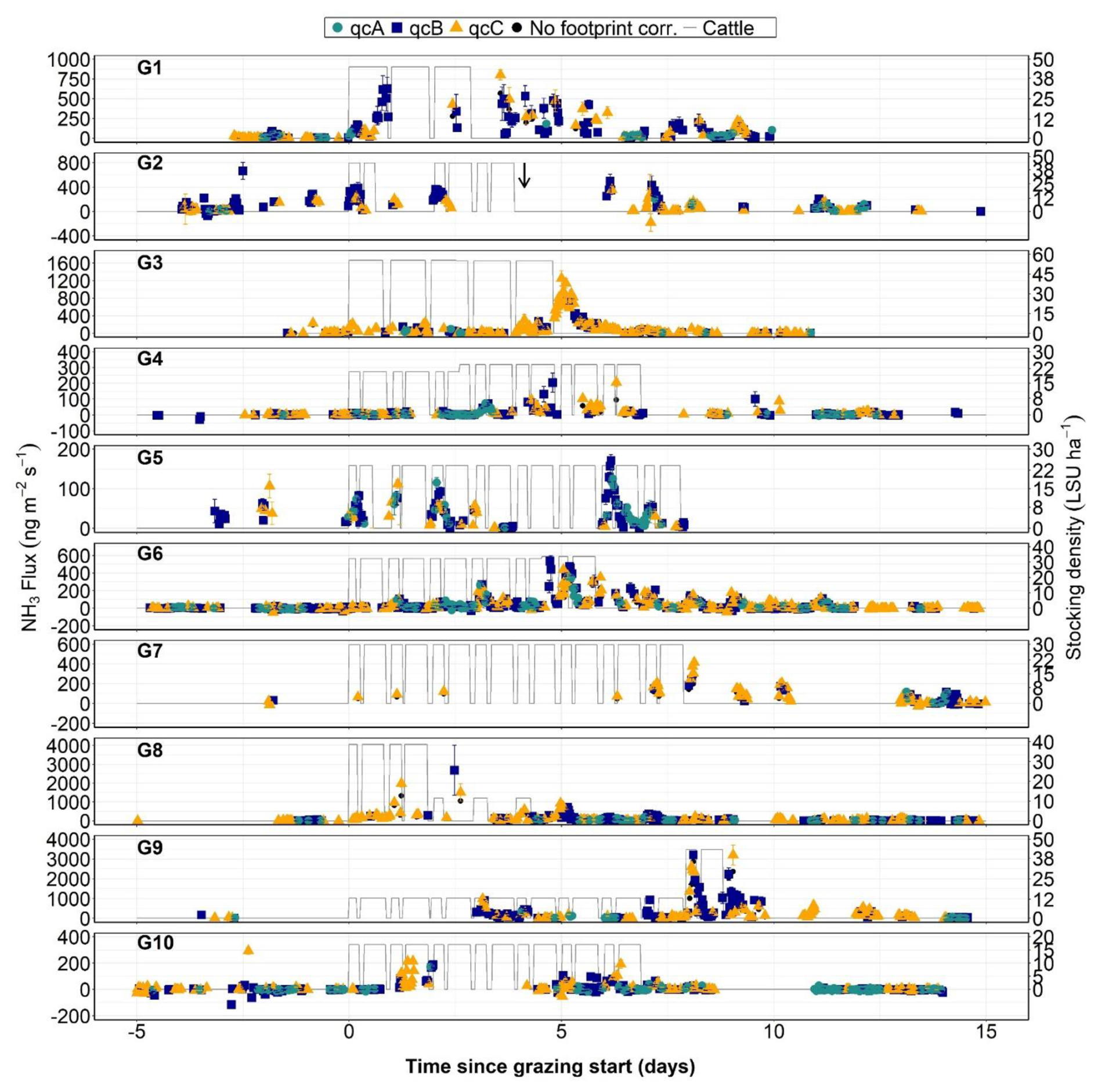
Figure 4 Temporal patterns of grazing-induced NH₃ fluxes (symbols) and stocking density (grey lines), measured up to 15 d after the onset of grazing for the 10 events summarised in Table 2. Coloured symbols (green circles, blue squares, orange triangles) show final corrected fluxes for the plot of interest in three quality classes (qcA, qcB, qcC, respectively, as defined in Table 1), with error bars showing random errors calculated from Eq. (10). For comparison, black circles indicate the same fluxes without footprint correction. The arrow in G2 indicates a fertilisation application of 39 kg NH₄NO₃-N ha⁻¹ that occurred just after grazing ended. Note that different y-axis scales are used due to variations in flux magnitude between grazing events.

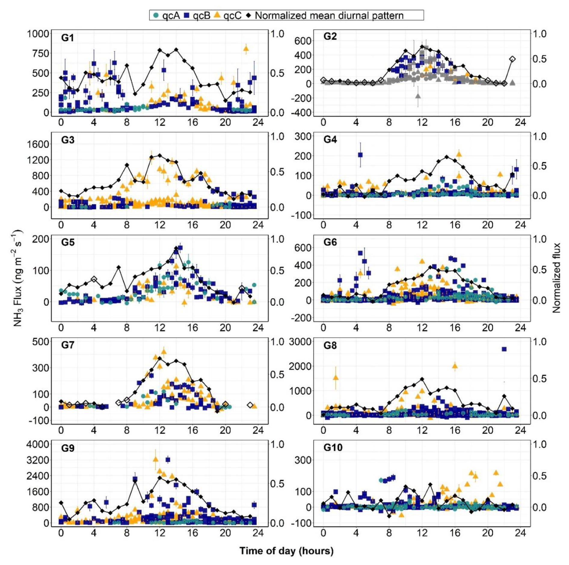
Figure 5 Diurnal variations of NH₃ fluxes for the 10 grazing events summarised in Table 2. Coloured symbols (green circles, blue squares, orange triangles) show final corrected fluxes in three quality classes (qcA, qcB, qcC, respectively), with error bars showing random errors calculated from Eq. (10). The black line shows the mean normalised diurnal flux pattern calculated using the DVmax method (Eq. S1 and Fig. S12). Black diamonds indicate hourly averages based on more than three data points; unfilled diamonds represent averages based on fewer than three. Fluxes measured after the mineral fertilisation event in G2 are shown in grey. Note that different y-axis scales are used due to variations in flux magnitude between grazing events.

Fluxes measured during and shortly after grazing ranged from −113 to 3205 ng NH₃ m⁻² s⁻¹, with the largest flux recorded during G9 (2024). Across the 10 grazing events (Table 2), NH₃ emissions followed distinct temporal patterns, with larger emissions during daytime than at night (Fig. 5), and often but not systematically peaked toward the end of the grazing phase, before gradually returning to background levels within a week or two after cattle departure (Fig. 4).

The largest half-hourly flux levels observed during each of the 10 grazing events varied between around 200 ng NH₃ m⁻² s⁻¹ (see G4, G5, G10 in Fig. 4) and 3000 ng NH₃ m⁻² s⁻¹ (G8, G9), with more common event-based peak levels around 500–1000 ng NH₃ m⁻² s⁻¹ (G1, G2, G3, G6, G7). For comparison purposes, the flux time series are also shown in Fig. S7 without footprint corrections, highlighting the importance of the footprint in data interpretation. For some grazing events (e.g. G2, G7, G8), the valid flux data capture was patchy mostly because the wind was blowing from unsuitable directions; the flux data thus discarded due to the footprint (shown as grey crosses in Fig. S7) may be fully representative of the adjacent plot (A or B, depending on which is the plot of interest) or a mixture of both plots, highlighting the difficulty of characterising temporal flux patterns in rotational grazing with one single flux measurement setup located on the divide. Over the 10 grazing events, around 75 % of the measured fluxes were net emissions (during the first 2 weeks following the start of grazing). These reinforce the hypothesis that grazing is a primary driver of NH₃ emissions, significantly increasing fluxes compared to background conditions.

3.4 Environmental controls on NH₃ fluxes

Apart from cattle slurry spreading, which triggered large but short-lived NH₃ emission pulses (see fluxes on 31 May 2022 in Fig. S4), the primary driver of NH₃ emissions on the pasture was the presence of grazing animals on the field. Measurement of ammonium and nitrate content in different topsoil strata from 0 to 30 cm depth showed a clear enhancement of mineral N as a result of grazing in 2023 and 2024 (Fig. S11). However, as shown in Fig. 4, the observed emissions did not occur systematically when animals were present, nor did the peak fluxes in each event scale with the stocking density during the grazing phase. Thus, apart from the supply of labile N to the soil through animal excreta, which can be assumed in the first approximation to scale with stocking density multiplied by the grazing duration (effective grazing days or EGD in Table 2), other environmental control factors must be invoked to explain the observed dynamics within each grazing event and the differences between the 10 grazing events.

Clear differences in fluxes between day and night hint strongly at control factors that vary diurnally, i.e. primarily meteorology. Because animals grazed on the field both day and night, apart from 2 h in the early morning and evening in the milking parlour, animal presence can be ruled out as the driver of day–night differences. The distinct diurnal cycle in NH₃ emissions in most of the 10 grazing events is shown in Fig. 5, with fluxes peaking in the afternoon (12:00–16:00 UTC+1) and declining overnight (00:00–06:00 UTC+1). Meteorological variables with marked diurnal patterns include air (and soil) temperature, relative humidity, VPD, global and net radiation, wind speed, and atmospheric turbulence (u_∗) and stability/instability (L), all known to influence the surface–atmosphere exchange of NH₃ (Flechard et al., 2013). Following standard thermodynamics of the equilibrium between aqueous-phase NH${}_{\mathrm{4}}^{+}$ and gas-phase NH₃, lower nighttime fluxes are consistent with reduced volatilisation under cooler conditions and higher relative humidity. Correlation analysis indicated that several meteorological variables were significantly correlated with NH₃ fluxes (Tables S3 and S4). Vapour pressure deficit and relative humidity indeed frequently showed a significant correlation (p<0.01) with NH₃ fluxes, especially during periods such as G4 and G6 (Fig. 6), but this pattern was not isolated to VPD and RH alone. Temperature (air and soil), wind speed and friction velocity also exhibited significant positive correlations (p<0.01) across several grazing events (see Figs. S8–S10).

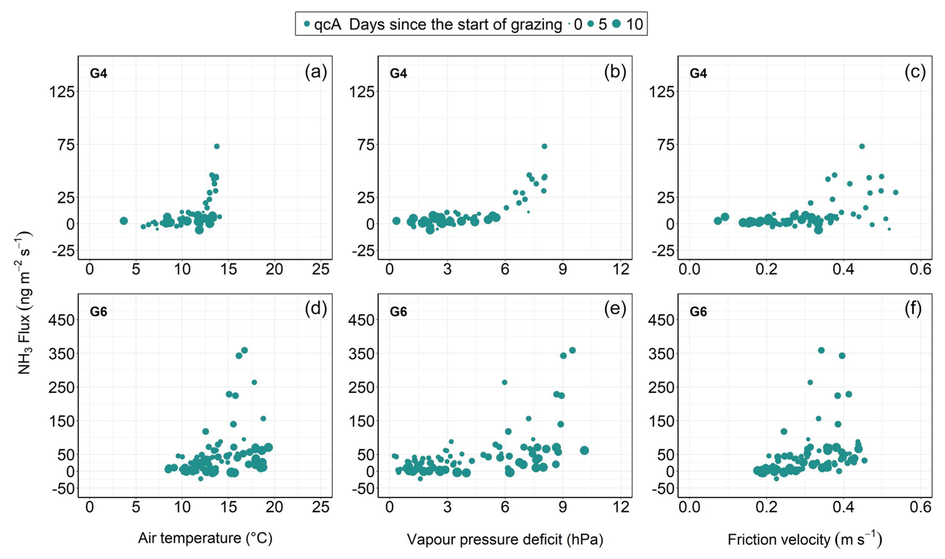
Figure 6 Relationship between NH₃ fluxes and air temperature (a, d), vapour pressure deficit (b, e) and friction velocity (c, f) for grazing events G4 and G6. Half-hourly qcA fluxes are shown, represented by green circles. Symbol sizes correspond to the time elapsed since grazing started. Note: different y-axis scales are used due to variations in flux magnitude between grazing events.

However, the aforementioned potential (micro-)meteorological drivers are often intercorrelated, positively or negatively on a diurnal basis: higher temperatures typically occur in the daytime at the same time as high VPD, low RH, unstable atmospheric conditions and large friction velocity (and vice versa at night). Therefore, this multi-collinearity implies that NH₃ emissions are modulated by the combined influence of several meteorological factors rather than a single dominant driver.

By contrast, soil moisture does not exhibit a systematic diurnal cycle but responds to rainfall and evapotranspiration over longer timescales (days to weeks). Precipitation events appeared to reduce emissions in particular during some grazing periods (e.g. G4), possibly by increasing surface wetness and physically limiting NH₃ volatilisation by reducing soil pore diffusivity, but also possibly because rainfall often coincided with cooler conditions and lower VPD. Conversely, the largest grazing-related NH₃ fluxes in spring 2022 (peak on 25 May 2022, phase G3) occurred 1 d after the end of a cumulative rainfall episode of 30 mm (Fig. S4), which may have triggered a large emission response.

3.5 Uncertainties in measured fluxes

Over the 10 grazing events, Fig. 4 and Table 2 show a roughly equal distribution of fluxes between the qcB (46 %) and qcC (38 %) classes (“good” and “modest” quality) but much fewer occurrences of qcA (“best” quality) fluxes (16 %). The mean relative random error in AGM NH₃ fluxes across the 10 grazing events ranged from 15 % to 72 %, with a mean overall value of 35 %, with u_∗ contributions to total random uncertainty ranging from 17 % to 64 %, while the error in the stability-corrected NH₃ gradient was larger, contributing from 36 % to 83 % (Table S2).

Systematic errors in AGM-derived fluxes are more difficult to quantify. Storage change errors were small (median relative error: 1.4 %; values smaller than 10 % (20 %) in 82 % (89 %) of cases). No flux data for chemically interacting pollutants were available to quantify gas-to-particle interconversion (e.g. reaction of NH₃ with HNO₃ to form NH₄NO₃ aerosol or evaporation of volatile NH${}_{\mathrm{4}}^{+}$ aerosol), but this effect was assumed to be small at this rural agricultural site, where NH₃ concentration was much larger than chemically interacting acids (the mean molar ratio of NH₃ to the sum of strong acids [HNO₃+ SO₂+ HCL] measured by DELTA^® was 11.2). By contrast, horizontal advection was likely a larger source of systematic error. Two effects may be distinguished: (i) advection of NH₃ plumes from local farms and animal housing buildings, the local dairy farm being located approximately 300–400 m to 120–140° SE, which, however, was not a dominant wind direction during the study (Fig. 1), and (ii) differential footprints of the different measurement heights in the vertical concentration profile and their location in relation to the finite-sized field.

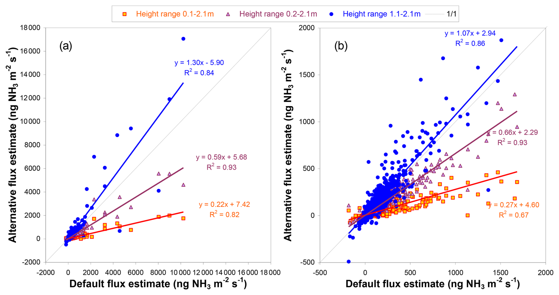
Figure 7 Sensitivity of NH₃ flux estimates to measurement height selection for (a) the whole flux dataset, including slurry-spreading events, and (b) fluxes only up to 2000 ng m⁻² s⁻¹ (more characteristic of grazing-induced emissions). Default fluxes (x axis) are based on the default height range used for flux calculation (0.5–2.1 m), while alternative fluxes (y axis) are calculated using 0.1–2.1 m (orange squares), 0.2–2.1 m (purple triangles) and 1.1–2.1 m (blue circles). Regression lines illustrate deviations from the 1:1 line (dashed), highlighting strong underestimation if the lowest measurement heights were included.

One way to assess the potential influence of advection and concentration footprint issues over the field is to calculate AGM fluxes using different measurement height ranges to compute Eq. (3). As shown in Fig. 7, there were systematic biases in fluxes computed from different height ranges, compared with the default flux estimates that used the range 0.5–2.1 m. Fluxes estimated from the full profile down to the lowest height (0.1–2.1 m) were consistently lower, with regression slopes of 0.22–0.27, indicating a 73 %–78 % underestimation. With the lowest height excluded (range 0.2–2.1 m), the underestimation was less pronounced, with regression slopes of 0.59–0.66 (34 %–41 % lower than the default). Fluxes derived from the upper two heights only (range 1.1–2.1 m) were 30 % larger than the default estimate if the whole dataset was considered (including the few very large slurry spreading-induced emissions); however, for lower flux magnitudes (< 2000 ng m⁻² s⁻¹), as typically observed during grazing, this height-dependent bias was greatly reduced to approximately 7 %.

Table 3 Cumulative NH₃ emissions (g N ha⁻¹) and emission factors (per livestock unit and fraction of the excreted N) for eight grazing events. Cumulative fluxes were calculated using the DVmax and DVavg gap-filling methods based on mean diurnal variation (see Methods). Grazing events G2 and G7 were excluded from cumulative and EF estimation due to low data availability. The urinary N excretion was estimated following Sect. S7.

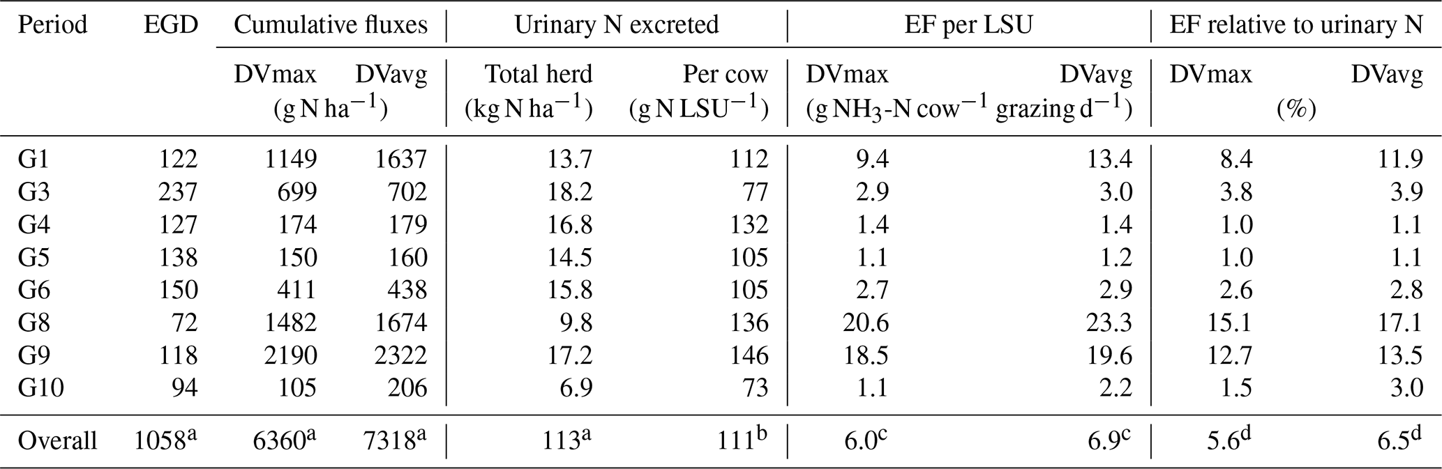
^a Sum over grazing events; ^b arithmetic mean over grazing events; ^c calculated as the ratio of sum total emission to sum total EGD; ^d calculated as the ratio of sum total emission to sum total urinary N excretion.

3.6 Grazing event-based cumulative fluxes and emission factors

Given that emissions typically returned to baseline within 15 d, cumulative flux estimates were calculated over this interval (Table 3), based on the gap-filling procedure described previously (see complete time series in Figs. S13–S14). Cumulative 15 d NH₃ emissions ranged from 105 to 2190 g N ha⁻¹ using the DVmax method and 160 to 2322 g N ha⁻¹ using the DVavg method. Cattle head-based EF values showed substantial variability, ranging from 1 to 21 g NH₃-N cow⁻¹ grazing d⁻¹ for DVmax and 1 to 23 g NH₃-N cow⁻¹ grazing d⁻¹ for DVavg. A more robust mean overall EF of 6.0–6.9 g NH₃-N cow⁻¹ grazing d⁻¹ was calculated as the ratio of the sum of all emissions to the sum of all EGD cumulated over the available eight grazing events (see last line of Table 3). Similarly, the EFs based on the fraction of deposited N emitted as NH₃ ranged from 1 % to 15 % and 1 % to 17 % for DVmax and DVavg, respectively.

4 Discussion

4.1 Methodological uncertainties and limitations in AGM flux measurements

4.1.1 Systematic versus random errors in AGM flux measurements

Random and systematic errors are influenced by instrument limitations, methodological assumptions and environmental variability (Brümmer et al., 2022). Standard random error analysis likely reflects the smaller fraction of the overall uncertainty. Systematic errors associated with the AGM have been discussed in previous papers (Fowler and Duyzer, 1989; Sutton and Fowler, 1992; Loubet et al., 2013) and are likely substantially larger, though much more difficult to quantify. Some systematic errors are related to NH₃ sampling and detection, and others to measurement conditions that invalidate the universal assumption that the vertical flux is constant with height, namely, chemical production or consumption of NH₃ between the measurement height and the surface, storage changes in the air column (Eq. 7), footprint heterogeneity, and horizontal advection.

4.1.2 Effects of the NH₃ sampling line

Ammonia is a notoriously difficult gas to sample and analyse (Ellis et al., 2010). In this study, standard calculations of the relative error from random sources (Eqs. 10–11) provided average values in the range 15 %–72 % of the absolute flux, based on turbulence sampling limitations and dispersion in NH₃ concentration gradient slopes. The AGM requires accurate gradient measurements, and NH₃ adsorption onto sampling tubes and instrument surfaces very likely produced some smoothing of high-frequency concentration changes and carryover of NH₃ from one sampling height to the next, despite equilibration times at each height (Fig. S1). This effect likely occurred despite a large sampling flow rate and a single heated and insulated sampling line used to minimise condensation and accumulation/loss effects. Such processes always result in an underestimation of vertical gradients, whether positive or negative, but the gradient (flux) underestimation was likely more pronounced during the night and in any other cool, humid conditions than during dry daytime conditions. The observed diurnal cycles in fluxes during grazing events (Fig. 5) may, for this reason, be exaggerated; emissions may have, in reality, been larger at night than the data suggest. On the other hand, the measurement system was often able to detect deposition gradients in background conditions, even during nighttime cool and high-humidity conditions (e.g. Fig. 2a). Overall, no objective criteria (e.g. comparison to another independent flux measurement system) was available to us to quantify the magnitude of the NH₃ “stickiness” effect.

4.1.3 Fundamental assumptions in AGM

A key source of uncertainty in this study involved the determination of a suitable concentration measurement height range, within the whole vertical profile (0.1–2.1 m) of the mast lift system, that could be considered at equilibrium with the upwind footprint within the pasture field. Low measurement heights on the mast are highly influenced by the near field, while upper heights look further upwind; a standard requirement in AGM is a homogeneous upwind fetch up to a certain distance, i.e. that the near field and far field have similar characteristics for soil, vegetation, roughness, etc. Fluxes computed using measurements including and above 0.5 m were adopted in our study as the best estimate because the lower two heights (0.1 and 0.2 m) were considered to be influenced by the ungrazed area within the enclosure surrounding the flux tower and ancillary equipment. This hypothesis was consistent with vertical profile observations such as Fig. 3b, often showing a deviation of the two lowest heights from the assumed log-linear profile development within the inertial sublayer.

More importantly, the Monin–Obukhov similarity theory is considered applicable only above the roughness sublayer, or RSL (Högström, 1996). The exclusion of the lower heights (0.1–0.2 m) from the vertical gradient slope calculation was consistent with the AGM requirement that vertical profiles be measured in the inertial sublayer, well above the RSL. Given that the RSL depth is estimated to be 1.5–2.5 times the canopy height (Melman et al., 2024), and with a typical grass height of 0.1–0.2 m in our study, the lowest 40–50 cm of the profile should be (and were) excluded from flux calculations.

For technical reasons, the 0.5 m measurement height was no longer available for flux calculations from May 2023 onwards, reducing the available profile heights to 1.1 and 2.1 m (Sect. 3.5). However, the reasonable agreement for moderately large fluxes (up to 2000 ng m⁻² s⁻¹; slope 1.07, Fig. 7b) between the default height range (0.5–2.1 m) and the upper two heights only (1.1–2.1 m) supported the hypothesis that potential horizontal gradients and differential concentration footprints did not greatly bias fluxes, despite the relatively small field size and upwind fetch (100–150 m for the main wind SW and NNW directions; see Fig. 1).

Nevertheless, spatial heterogeneity arising from uneven grazing, rumination and urination behaviours likely resulted in localised concentrated urine deposition (N hotspots) within the pasture. When located upwind of the flux measurement tower, such hotspots would invalidate the assumption of near-field/far-field homogeneity, and depending on whether the hotspots were close to the tower or further upwind, the resulting emission gradient would have been overestimated or underestimated. Whatever the case may be, the heterogeneous distribution of deposited urine-N inherent in grazed grasslands was certainly an important factor in increasing the uncertainties associated with AGM-derived estimations.

The classical AGM assumes that eddy diffusivities for momentum (K_M) and scalars (K_H) are equal under neutral and stable conditions (Thom, 1975), but this assumption has been challenged in more recent studies (Flesch et al., 2002; Stull, 2012; Wilson, 2013; Foken, 2006). Further, the stability corrections, derived for vertical scalar profiles derived in the 1960s–1970s (e.g. Dyer and Hicks, 1970), have been re-evaluated in several publications (e.g. Högström, 1988; Foken, 2006). They were found to be acceptable within the margin of instrumental error for moderately unstable conditions but more questionable for stable conditions and very unstable conditions, although no universal consensus has yet been found (Högström, 1996). Such uncertainties imply that traditional AGMs could be biased with respect to flux calculations (Anderson et al., 2019). Although this study retains the original AGM assumptions and stability correction functions from the 1970s, we recognise that potential deviations may have introduced additional uncertainty in our flux estimates.

4.1.4 Footprint-derived corrections of measured fluxes

The flux correction procedure based on footprint modelling and attribution (Sect. 2.4.5) introduced further uncertainty related to the accuracy of the spatial extent of the footprint and resistance parameterisations used in the estimation of background fluxes (Eqs. 8–9 and Fig. S16). Sintermann et al. (2012) recommended considering that at least half of the flux footprint must originate from a given field for accurate flux assessment. We used a more severe threshold of two-thirds for each half-hourly flux footprint to originate from the relevant field. The resistance-based flux model used in this study to simulate background exchange was meant to address the potential emission underestimation from incomplete flux footprint coverage, but model resistance parameterisations come with significant uncertainties of their own. A combined approach integrating AGM measurements with other independent flux measurement methods (EC, bLS inversion, etc.) could improve NH₃ flux assessments in future studies.

4.2 Ammonia exchange dynamics in relation to grazing–soil–ecosystem interactions

The magnitude of NH₃ emissions is controlled by environmental and management factors reflecting the interplay of dairy and grazing management, nitrogen distribution, and atmospheric conditions (Jarvis et al., 1991). During grazing, NH₃ fluxes exhibited a characteristic gradual increment, often peaking either toward the end or shortly after cattle departure before declining within a week. This pattern, observed across multiple grazing events, aligns with previous studies (Bell et al., 2017; Jarvis et al., 1989b; Laubach et al., 2013; Voglmeier et al., 2018), highlighting how the combined effects of excreta deposition (labile N addition to soil), vegetation disturbance and atmospheric conditions (weather and turbulence) interact to shape NH₃ emission dynamics.

The dominant driver of NH₃ emissions during grazing is considered to be urine deposition, which introduces large amounts of nitrogen as urea in concentrated patches and elevates soil pH, especially in the uppermost soil layer (see Fig. S11). Urea hydrolysis drives ammoniacal nitrogen release and promotes gas-phase NH₃ evolution (Giltrap et al., 2017; Laubach et al., 2013; Selbie et al., 2015). Apart from meteorology, the extent of NH₃ release is strongly influenced by several intrinsic ecosystem factors, including soil pH and cation exchange capacity. In this study, late-winter pre-season pH values were in the range of 5.5–6, but values measured during or after grazing often reached 6.5–7 (Fig. S11).

In addition, herbage nitrogen content affects the nitrogen composition of excreta (Jarvis et al., 1989a, b). In this study, high herbage N in G1 (3.1 %; see Table 2) coincided with large volatilisation from deposited urine, which may indicate the role of excreta quality in driving emissions, although this is difficult to confirm given other confounding factors such as meteorology. The interaction between vegetation and soil NH₃ emissions further modulates fluxes. Before grazing, dense canopies absorb atmospheric NH₃ through stomatal uptake and non-stomatal deposition (Asman et al., 1998; Flechard et. al., 2013; Harper et al., 1983). Grazing disrupts the balance by reducing biomass, shortening canopy height and decreasing leaf surface area available for NH₃ recapture, leading to increased net emissions. This effect was particularly evident in G1, G4 and G6, where peak fluxes coincided with cattle departure when the canopy was most reduced (Figs. S4c–S5c). The removal of taller vegetation increases wind penetration into the canopy and re-couples the atmosphere with the soil surface, facilitating rapid vertical NH₃ transfer (Denmead et al., 1976). After cattle removal, plant regrowth resumes and reduces soil emissions by the double effect of root N uptake and canopy recapture of soil-emitted NH₃.

Nonetheless, post-grazing fertilisation raises the N status of the system and the stomatal compensation point (Loubet et al., 2002), promoting potential NH₃ emission by leaves. We frequently observed bi-directional exchange in background conditions, including small net ecosystem emissions (up to $\sim +\mathrm{50}$ ng m⁻² s⁻¹), even after several weeks following the latest grazing or fertilisation event (Figs. S3, S16). Soil nitrogen levels post-grazing are also influenced by competing soil microbial processes, including nitrification and denitrification, which further regulate NH₃ volatilisation (Selbie et al., 2015).

Cattle movements on the field play a role in regulating NH₃ dynamics through the spatial distribution of excreta. Exceptionally large NH₃ fluxes were observed in spring 2024 (with peaks exceeding 2000 ng m⁻² s⁻¹) and may be partly explained by observations showing that cattle often aggregated near the water trough SSW upwind of the measurement system, leading to localised nitrogen hotspots, a well-documented driver of flux variability (Bell et al., 2017; Laubach et al., 2013). In G8, such an aggregation effect would be consistent with the large spatial variability in topsoil NH${}_{\mathrm{4}}^{+}$ observed post-grazing (Fig. S11). Uneven nitrogen distribution may have contributed to some of the NH₃ peaks, but only if flux footprint areas coincided with N hotspots, which could not be verified experimentally. Soil compaction from trampling on such hotspots may have influenced emissions by reducing infiltration, leading to longer retention of urine on the surface (Luo et al., 2017) and prolonged NH₃ volatilisation properties. The introduction of a second cattle group in G9 (43 LSU ha⁻¹ after 7 d of initial grazing at 13 LSU ha⁻¹) likely enhanced N deposition, contributing to the strong increase in observed emissions.

4.3 Effect of meteorology

Previous studies have highlighted the challenge of linking NH₃ fluxes directly to meteorology due to the strong interdependence of environmental variables (Jarvis et al., 1991). In this study, temperature, relative humidity, vapour pressure deficit (VPD), wind speed and turbulence (u_∗) were all strongly correlated with NH₃ fluxes (Table S3), but cross-correlations on a diurnal basis between these variables make it difficult to isolate single effects, especially because a further dimension (time) is needed to characterise the very strong dynamics of soil nitrogen and vegetation LAI and canopy height in response to grazing over 1–2 weeks.

Temperature influences NH₃ volatilisation directly by modulating substrate availability in the urine patch through urease activity and by controlling the aqueous/gaseous-phase partitioning of ammoniacal nitrogen (Reynolds and Wolf, 1987). It also has indirect effects through elevated VPD, which accelerates soil surface evaporation and plant transpiration, also forcing NH_x out of the aqueous phase at the soil–plant–atmosphere interface. This effect was particularly evident in G4 and G6, where high VPD levels coincided with peak emissions (Fig. 6). Conversely, low VPD conditions (or high relative humidity) are associated in the literature with enhanced deposition onto plant and soil surfaces promoting non-stomatal NH₃ uptake surfaces and further suppressing net volatilisation to the atmosphere (Bell et al., 2017; Flechard et al., 2013; Freney et al., 1983), which appears to be consistent with the observed flux patterns. Cooler nighttime temperatures also slow urea hydrolysis.

Nevertheless, several nighttime data points exhibited relatively high NH₃ emission gradients (sometimes up to tens of µg NH₃ m⁻³ difference between measurement heights, for example, during G8), which, despite very low turbulence ($u_{\ast }<\mathrm{0.05}$ m s⁻¹), yield high emissions calculated from the flux–gradient equation. In such intermittent turbulence conditions, the uncertainty in the AGM flux is very large, even though they passed all criteria in the flux selection procedure (see Sect. 2.4.4), albeit with many data points assigned qcC (modest quality). Such data should not be overinterpreted or even could be treated as outliers, but the data nonetheless suggest that under stable night conditions, NH₃ may accumulate near the surface during temperature inversions, trapping emissions closer to the ground due to reduced atmospheric mixing and limited vertical NH₃ transport. When minimal turbulence resumes, this accumulated NH₃ may be transported and released, resulting in spikes that might not represent instantaneous emission processes but rather delayed transport of previously emitted NH₃.

The impact of precipitation on NH₃ fluxes is ambiguous. Heavy precipitation is likely to reduce emissions by diluting urea from urine patches, lowering NH${}_{\mathrm{4}}^{+}$ concentrations at the soil surface and enhancing infiltration (Harper et al., 1983; Walker et al., 2013); this possibly happened in G4 (Fig. S5). However, rain falling on dry soil, as in the case of G3 (Fig. S4), may temporarily promote a pulse of NH₃ emissions by dissolving surface nitrogen, facilitating urea hydrolysis and microbial activity, and increasing TAN availability (Sommer et al., 2004).

Apart from meteorology, the main challenge in explaining the temporal variations in half-hourly NH₃ fluxes was the lack of measurements, or even proxies, to describe the short-term dynamics in soil surface TAN. This is the only variable that can explain the typical pattern of increase, peak, then decrease in emissions over 1–2 weeks (Fig. 4). Without high-enough-resolution (say, daily) TAN data, no multivariate regression analysis can hope to capture, or predict, these flux patterns.

4.4 Variability in emission factors in this and other studies

Grazing-induced NH₃ fluxes in this study persisted for several days and were larger than those observed following NH₄NO₃-N fertiliser applications (Figs. S4–S6). The estimated nitrogen input from individual grazing events (7–22 kg N ha⁻¹) was lower than that from mineral fertilisations (28–49 kg N ha⁻¹); however, cumulative NH₃ emissions were often higher under grazing. This highlights the significance of grazing as a field-scale NH₃ source. Our findings underscore that grazing with its high volatilisation potential from urine patches is still a critical ecological contributor to NH₃ emissions under field conditions. Even so, grazing is often considered a mitigation strategy relative to confined animal feeding operations.

The mean cattle head-based EF we derived from eight grazing events was 6–6.9 g NH₃-N cow⁻¹ grazing d⁻¹ but with very large variability (factor of ∼1 to 20). With only eight EF values derived from our dataset (Table 3) and almost as many potential explanatory macro-drivers (soil/air temperature, VPD or RH, wind speed or u_∗, rainfall, cattle diet or herbage N content), no statistical multivariate analysis could be applied to derive the share of EF variance explained by individual variables. This would be all the more difficult due to cross-correlations between meteorological drivers.

Table 4 Comparison of NH₃ fluxes, grazing event-based emission factors (EFs) and measurement methodologies in grazed grassland studies. Mixed vegetation refers to grasslands with a ryegrass-clover sward.

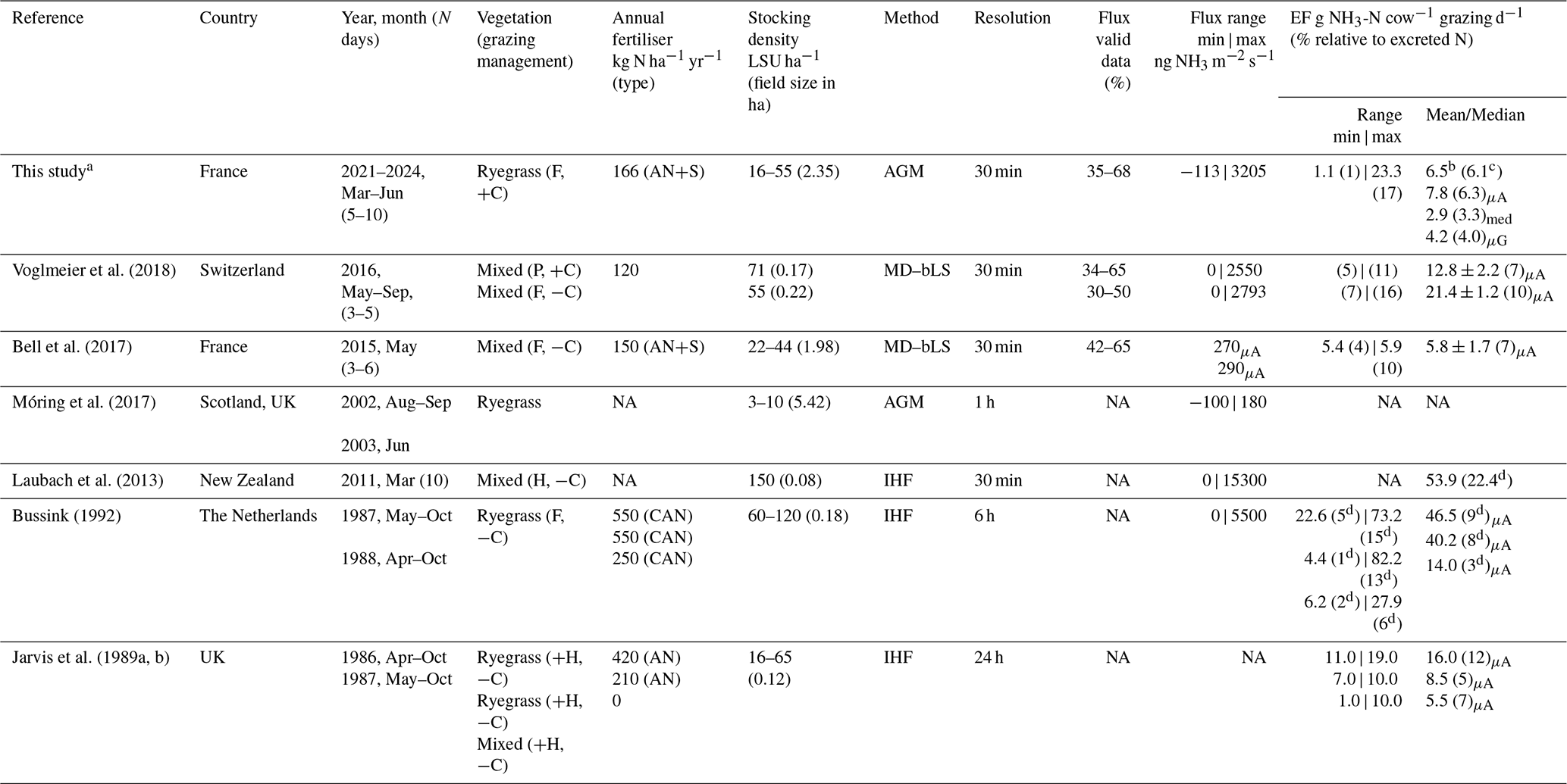
^a Mean overall EF values computed from the average of the DVmax and DVavg gap-filling methods.
^b Calculated as the ratio of sum total emission to sum total EGD (see Table 3).
^c Calculated as the ratio of sum total emission to sum total urinary-N excretion (see Table 3).
μA: arithmetic mean of individual event-based EFs; μG: geometric mean of individual event-based EFs; med: median of individual event-based EFs.
^d Percent % N relative to total excreted N as urine and dung.
N days: days considered to compute EF after cattle departure.
Pasture management: F – full-time grazing; P – part-time grazing; H – harvested pasture.
Grazing with other diet complementation (+C) and without (−C).
Fertilisation: S – slurry; AN – ammonium nitrate; CAN – calcium ammonium nitrate.
Measurement methods: MD–bLS refers to miniDOAS combined with bLS backward Lagrangian stochastic model, and IHF refers to integrated horizontal flux.
NA: not available.

In 2024, NH₃ EF peaked at 19–23 g NH₃-N cow⁻¹ grazing d⁻¹ during G8–G9, but the available data do not offer any obvious explanation for these large values. Most of the EF estimated at our site fell within the range of other studies (Table 4), in which the largest values of 53.9 g NH₃-N cow⁻¹ grazing d⁻¹ were measured in conditions of very large stocking density (Laubach et al., 2013). However, the variability observed in grazing-induced emissions remains relatively small compared to that reported from dairy buildings, where EFs can range from 0.7 to 205.9 g NH₃-N cow⁻¹ d⁻¹ (Hristov et al., 2011).

Valid flux data capture at our site was, on average, around 40 % (range 18 %–68 %) across the 10 grazing events, in large part due to footprint issues associated with the division of the field into two grazing paddocks, with the measurement setup in the centre. Thus, gap-filling accounted for 60 % of the time on average. It follows that the uncertainty in the cumulative fluxes and EF depends to a large extent on the accuracy of the simple statistical gap-filling procedure we used. The difficulty in explaining the variations in EFs between grazing events is possibly also a reflection of the uncertainty in gap-filling. EF values, as the most synthetic, high-level product of the study, combine all the individual uncertainties of lower-level variables and should be interpreted with caution.

Ammonia emissions from grazed grasslands vary significantly between studies not only due to differences in management and environmental factors but also due to potential differences and biases between measurement techniques. Early mass balance methods (e.g. integrated horizontal flux using filter packs) lacked the temporal resolution needed to resolve short-term grazing emissions, requiring extensive manual sampling. Automated higher-frequency measurement techniques, such as quantum cascade laser spectroscopy, wet denuder with online analysis, or miniDOAS applied to eddy covariance, AGM or backward Lagrangian stochastic (bLS) inversion, have advanced NH₃ flux monitoring. Nevertheless, methodological inconsistencies still limit cross-study comparisons, as was shown by Sintermann et al. (2012) in the case of field slurry spreading.

Paired miniDOAS systems with bLS have been applied to grazed grasslands (Bell et al., 2017; Voglmeier et al., 2018). Laubach et al. (2013) used a mass balance approach, while Laubach et al. (2012) focused on artificial urine patch studies. The fluxes and EF observed at the field scale in this study align with those of Voglmeier et al. (2018) and Bell et al. (2017) in similar-sized fields (∼1–2 ha). Smaller paddocks may tend to yield higher NH₃ fluxes due to concentrated grazing and higher excretion density, while larger fields may dilute emissions. The largest cattle-based EF reported in Table 4 was obtained from measurements conducted in small demarcated fields (<0.1 ha) with livestock provided with a mixed diet (ryegrass clover mixture).

Vegetation type and fertilisation history significantly influence background NH₃ fluxes through internal N cycling and compensation point processes (Flechard et al., 2013). Our study site was dominated by ryegrass, whereas other studies included mixed swards with legumes such as white clover, which can alter nitrogen cycling and, in turn, urinary composition. Bussink (1992) demonstrated that excessive fertilisation (550 kg N ha⁻¹) increased NH₃ volatilisation due to higher urinary N content. Jarvis et al. (1989a) found a higher cattle head-based EF for an unfertilised ryegrass-clover mixture than for a 210 kg N ha⁻¹ fertilised ryegrass, suggesting that biological nitrogen fixation and associated changes in urine composition may contribute to increased NH₃ emissions.

The management of the experimental site in this study frequently includes organic and mineral fertilisation, as well as occasional cutting events for hay or silage harvest. Emissions from grass cuts can be comparable to grazing (Milford et al., 2009), while Spirig et al. (2010) reported peak NH₃ emissions from slurry application reaching 70 000 ng m⁻² s⁻¹, 20 times larger than peak grazing fluxes in this study. This highlights the importance of considering fertilisation types and doses, application methods, and all other aspects and fluxes related to pasture management if the goal is to describe the total net inter-annual NH₃ budget from the entire grazed, fertilised, cut grassland system, not just emissions occurring during grazing phases.

5 Conclusion

Long-term, high-resolution NH₃ flux monitoring datasets across diverse grazing systems and under different climatic conditions are essential for improving process understanding, refining emission estimates and reducing uncertainty in national and global emission inventories. This study presents one of the most extensive high-resolution datasets of field-scale grazing-induced NH₃ fluxes, capturing diurnal, seasonal and inter-annual variability. The data show that grazing in even moderately intensively managed grasslands can contribute larger cumulative seasonal fluxes than emissions from applied mineral or even organic fertilisers, depending on stocking density, vegetation characteristics and meteorological conditions.

The data indicate a very large variability in time-integrated emission factors per livestock unit between eight grazing events, rather at the low end of the range of values from the few other datasets found in the literature. Thus, they highlight the difficulty of generalising the results to national or continental scales. These differences underscore the role of site-specific conditions (meteorology, soil) and livestock management practices on NH₃ emissions.

Despite the extensive flux data coverage across 4 years and contrasting environmental conditions at our site, the emission variability could not be explained by the available data for the most likely meteorological, ecosystem and management drivers. Untangling the relative share of control by individual control factors through correlation (multivariate) analysis is practically impossible on the sole basis of in situ field observations, partly due to cross-correlations between drivers and the absence of high-resolution soil TAN data. This is also very likely partly due to the large uncertainties in measurement-derived EF estimates, which combine a long chain of random errors in individual measured variables, systematic errors in AGM (NH₃ sampling, advection, concentration footprint and uncertainties in Monin–Obukhov similarity theory), field-scale grazing heterogeneity, correction procedures (flux footprint attribution) and, finally, gap-filling methodology. Process-based models (e.g. Móring et al., 2017) offer a potential alternative to average or default EF values for upscaling but require robust observational datasets for calibration and validation. Future research should focus on (i) continued long-term NH₃ flux monitoring in grazed grasslands in diverse situations using a state-of-the-art methodology (e.g. open-path eddy covariance) and (ii) incorporating soil–vegetation–animal–atmosphere interactions into process-based models to improve NH₃ emission predictions and to provide mechanism-based EFs for spatial and temporal generalisation and prospective studies.