Evaluating the carbon and nitrogen cycles of the QUINCY terrestrial biosphere model using space-born optical remotely-sensed data

Accurate estimates of future land carbon sinks and thus the remaining carbon budget to achieve the Paris climate goals requires rigorous modelling of the carbon sequestration potential of the terrestrial biosphere. Estimating the terrestrial carbon budget requires an accurate understanding of the interlinkages between the land carbon and nitrogen cycles, yet coupled carbon-nitrogen cycle models exhibit large uncertainties. Leaf chlorophyll, chl_leaf, is an indicator of the leaf nitrogen content stored within photosynthetic nitrogen pools and is central to the exchange of carbon, water and energy between the biosphere and the atmosphere. In this work, we harness an advanced remote sensing (RS) chl_leaf product to evaluate a terrestrial biosphere model (TBM), QUantifying Interactions between terrestrial Nutrient CYcles and the climate system (QUINCY), which explicitly models chl_leaf. We focus on comparing the spatial and seasonal patterns of modelled and observed chl_leaf, and then further assessing if modelled leaf area and productivity agree with a RS leaf area index product and in-situ eddy covariance-based gross primary production, respectively. In addition, we conduct additional simulations to test two alternative formulations of leaf-internal nitrogen allocation within QUINCY. Our analysis over a globally representative set of locations reveals that QUINCY chl_leaf magnitudes are mostly in line with the RS chl_leaf values. However, QUINCY chl_leaf tends to show a narrower numerical range compared to RS for specific ecosystem types, such as grasslands. While the seasonal cycle of QUINCY chl_leaf mostly corresponds well to the observations, for many deciduous forests, the increase in QUINCY's chl_leaf predictions in spring and the decrease in autumn were delayed compared to observations. Our results also show that compared to the original leaf nitrogen allocation scheme of QUINCY, the revised scheme produced a more reasonable sensitivity of gross primary production to increases in chl_leaf. However, the revised scheme did not directly lead to improvement in simulating chl_leaf and gross primary production. Our study shows the value of RS products linked to nitrogen cycle that will be useful in both carbon and nitrogen modelling, and paves way for closer linking of RS and TBMs.

1 Introduction

The terrestrial biosphere currently takes up approximately one-third of the anthropogenic fossil fuel carbon emissions (Friedlingstein et al., 2023), and thereby playing pivotal role in slowing global climate warming (Nabuurs et al., 2022). The carbon (C) cycle is closely linked to the terrestrial nitrogen (N) cycle, as photosynthesis and plant growth require sufficient nutrient supply. Land carbon uptake is limited by nitrogen in many ecosystems (LeBauer and Treseder, 2008; Fisher et al., 2012; Tamm, 1991; Vitousek and Howarth, 1991; Ziehn et al., 2021), however, the magnitude of this limitation remains unclear. This highlights the need to better understand the coupled C and N cycles (Seiler et al., 2024), as future changes in climate will also affect these cycles (Arora et al., 2020).

Terrestrial biosphere models (TBMs) can be used to simulate coupled C and nutrient cycles and land-atmosphere interactions under a changing climate. In recent decades, TBMs have taken in an increasing number of factors affecting plant photosynthesis, such as nutrient limitation (Blyth et al., 2021). Whilst Kou-Giesbrecht et al. (2023) reported that TBMs are capable of reproducing the historical terrestrial C sink with a sufficient level of performance, uncertainties persist. TBMs use different modeling approaches to represent N limitation of photosynthesis and the effect of N availability on leaf N, which can lead to varying results regarding plant productivity (Medlyn et al., 2015). Leaf N can be obtained directly from soil N availability by using a fixed parameter or with flexible parametrization using leaf C:N ratios (Thomas et al., 2015). Increasing model complexity regarding modeling the N limitation can thereby also introduce further uncertainties into the estimates of the carbon sink (Fisher and Koven, 2020; Famiglietti et al., 2021), through both process and parameter uncertainty, given the inclusion of new process equations. These uncertainties are also reflected in significant divergence of N pools and fluxes modelled by the current generation of TBMs (Kou-Giesbrecht et al., 2023). In addition, the modelled responses of photosynthesis to elevated atmospheric carbon dioxide (CO₂) or to N deposition vary between different TBMs, requiring a better understanding of the N cycle (Davies-Barnard et al., 2020; Arora et al., 2020; Meyerholt et al., 2020; Zaehle et al., 2014). It is therefore important to better constrain the nitrogen dynamics in these models.

One of the major sources of uncertainty in modeling the land carbon sink with TBMs is the uncertainty in estimating the leaf photosynthetic capacity and photosynthetic rate (Bonan et al., 2011; Rogers et al., 2017). Leaf chlorophyll (chl_leaf) is intrinsically related to plant photosynthesis, due to its role in generating biochemical energy for the carboxylation reactions within the Calvin–Benson cycle, through the harvesting of solar radiation. Previous work has demonstrated that leaf chlorophyll content is a strong proxy for photosynthetic capacity (Croft et al., 2017; Lu et al., 2020; Luo et al., 2021). The maximum carboxylation rate at the 25 °C reference temperature (V_c(max),25) represents the limitation of photosynthesis by the Rubisco enzyme, which is the main regulator in light-saturated photosynthesis (Houborg et al., 2013). Due to the investment of N in chl_leaf molecules and an optimal N investment strategy to ensure close co-ordination between light-harvesting and carboxylation reactions, there is a close relationship between leaf N and chl_leaf (Sage et al., 1987; Evans, 1989). In-situ observations of chl_leaf can therefore be used to improve the parametrization of physiological schemes within TBMs to improve GPP estimates (Luo et al., 2018, 2019; Lu et al., 2022; Thum et al., 2025). However, many of the contemporary TBMs do not represent chl_leaf, and the widely used version of the FvCB model (Farquhar et al., 1980) for photosynthesis description does not explicitly take into account the role of chl_leaf in photosynthesis. In addition, the majority of TBMs only consider total canopy N and its vertical distribution (Vuichard et al., 2019; Best et al., 2011; Clark et al., 2011).

In addition to in-situ observations, remote sensing (RS) of the Earth's vegetation provides comprehensive data for evaluating TBMs. Leaf nitrogen is difficult to retrieve directly from RS observations (Farella et al., 2022), in comparison to chl_leaf which is more feasible to derive remotely (Croft and Chen, 2018), due to the presence of large chlorophyll absorption features in visible wavelengths. The advantage of using remotely sensed chl_leaf is its global and seasonal coverage and relatively long time span, compared to in-situ observations. Similarly as in-situ observations, RS chl_leaf can be harnessed to improve the modeled photosynthetic processes which include V_c(max) (Houborg et al., 2013). For example, Liu et al. (2023) retrieved global daily V_c(max) for C3 biomes by using RS chl_leaf and RS solar-induced chlorophyll fluorescence. Another advantage of RS chl_leaf is that they are linked to space-borne observations of leaf area index (LAI), both retrievable remotely (Croft et al., 2020). This allows the modeled leaf surface area to be evaluated simultaneously with chl_leaf.

In this study, we utilized a spatial RS chl_leaf product (Croft et al., 2020) to evaluate the chl_leaf representation of the TBM QUINCY (QUantifying Interactions between terrestrial Nutrient CYcles and the climate system) (Thum et al., 2019; Caldararu et al., 2020), which has fully prognostic coupled carbon and nitrogen cycles. QUINCY includes an explicit representation of chl_leaf and its impact on photosynthesis, and also the photosynthetic parameters V_c(max),25 and the maximum electron transport rate at 25 °C reference temperature (J_max,25) are directly determined from leaf nitrogen. We analysed model performance with respect to the temporal and spatial distribution of chl_leaf and LAI in different ecosystems globally. We further compared the simulated gross primary production (GPP) with the ground-based measurements from eddy-covariance network stations. To understand model-data mismatch, we used a machine learning approach to analyze how different environmental drivers affect both QUINCY and RS chl_leaf. We further investigated whether the observed difference in chl_leaf between QUINCY and observations is related to modeled N limitation by examining QUINCY's leaf C:N values. Here we use RS data as a reference for evaluation, though we acknowledge that RS data are also simulated product and have different characteristics than in-situ data. In other words, our evaluation can be understood more as a comparison study between TBM and RS-derived data.

Initial results suggested that the modeled response of chl_leaf to leaf N was not realistic, foremost because the original leaf nitrogen scheme in QUINCY does not take into account of the observed relationship between chl_leaf and V_c(max) (Evans and Clarke, 2019). In order to have a more realistic representation, we formulated an alternative leaf N allocation scheme in QUINCY based on Onoda et al. (2017) and Evans and Clarke (2019), where the V_c(max) and chl_leaf ratio is taken into account, and compared the additional simulation results with the original leaf N allocation scheme.

The objectives of the study were to determine different methods for using RS chl_leaf in model evaluation and how RS chl_leaf can benefit modeling of coupled C and N cycles. The research questions addressed in this work are as follows:

• Are the spatial and temporal patterns of global chl_leaf in QUINCY and RS similar?

• Is QUINCY's performance in modeling chl_leaf related to its ability to produce measured annual GPP?

• What are the main environmental drivers that affect QUINCY chl_leaf and RS chl_leaf?

2 Materials and methods

In this section, we will first present the study sites and observational data, followed by QUINCY model description and simulation setup. Finally, a machine learning approach to determine chl_leaf environmental drivers is presented. In this study, chl_leaf denotes both chlorophyll a and b (chl_a+b). All the datasets used in the study are presented in Table S1 in the Supplement.

2.1 Description of the sites

We conducted the analysis using two different site sets. The first set was the Protocol for the Analysis of Land Surface Models (PALS) Land Surface Model Benchmarking Evaluation Project (PLUMBER2) (Ukkola et al., 2022). The second site set, GLOBAL, is based on the study by Caldararu et al. (2022).

PLUMBER2 (Abramowitz et al., 2024) was designed for serving in a model intercomparison project for land surface models, and provides CO₂ eddy covariance measurements and meteorological data for various sites. The time interval of PLUMBER2 site data varies depending on the site, as some of the site data cover only one year, while others cover over a decade. The time span of PLUMBER2 site data is between 1992–2018. Of the available sites, we included 143 PLUMBER sites that had RS chl_leaf, RS LAI and QUINCY data available, and that were not reported by Abramowitz et al. (2024) to have anomalous precipitation input data. The GLOBAL site set represents all major climate zones and global biomes, and the site input data is for the years 1989–2018 based on the CRU JRA dataset (Harris, 2020). In our analysis, we used 279 GLOBAL sites for which QUINCY simulations and RS chl_leaf data were available and matched in land cover type (see Sect. 2.2.3).

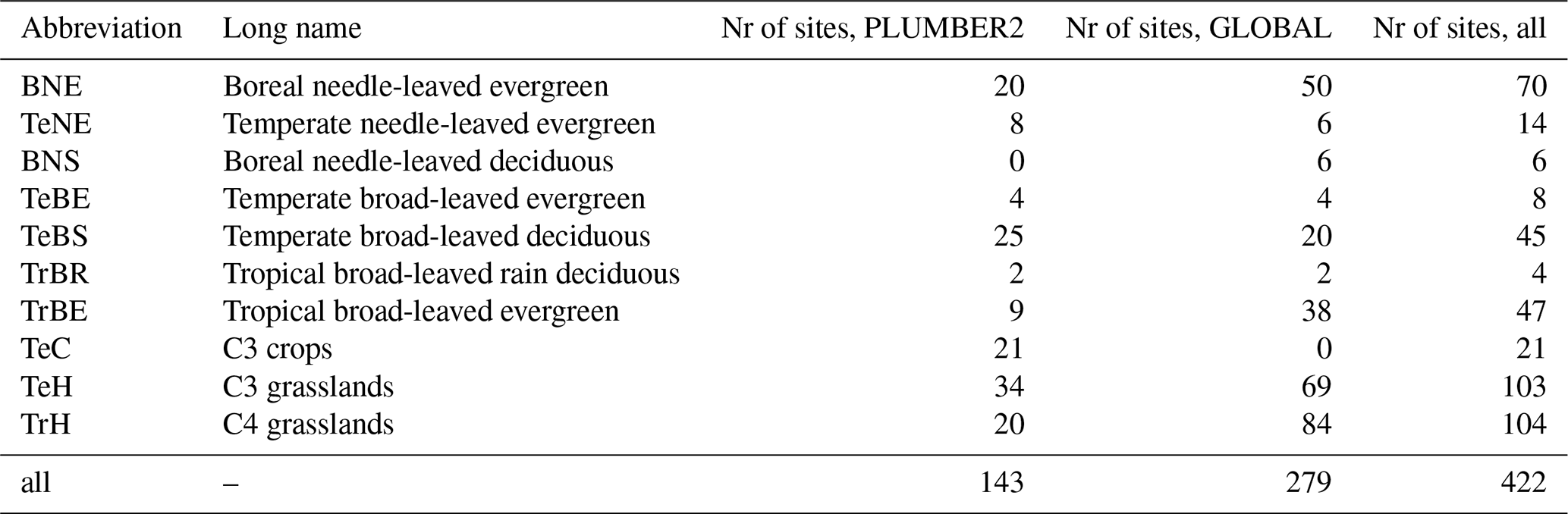
In total, the combined PLUMBER2 and GLOBAL analysis included 422 sites. The locations of the PLUMBER2 and GLOBAL sites are presented in Fig. S1 in the Supplement. The sites are categorized based on the QUINCY plant functional types (PFTs), and the number of GLOBAL and PLUMBER2 sites in each PFT are listed in Table 1.

Table 1 List of QUINCY PFTs and the corresponding number of sites in the PLUMBER2 and GLOBAL site sets.

2.2 Remote sensing data

2.2.1 Remotely sensed chl_leaf

We obtained chl_leaf content from the global RS product by Croft et al. (2020). The RS chl_leaf is derived from the ENVISAT MERIS full-resolution reflectance data with a two-stage radiative transfer model. The spatial resolution of the global RS chl_leaf is 300 m, and the data are processed to a 7 d temporal resolution for the years 2003–2011. The chl_leaf has been retrieved by first modeling the reflectance spectra at the leaf level using two separate models: the 4-Scale model (Chen and Leblanc, 1997) for forested and spatially clumped ecosystems, and the SAIL model (Verhoef, 1984) for cropland and grassland ecosystems. The chl_leaf has been then derived from the leaf reflectance spectra by using the PROSPECT leaf optical model (Jacquemoud and Baret, 1990). The influence of gaps has been partially minimized in the RS chl_leaf by Croft et al. (2020) by gap-filling the missing data with the year 2010 data and a smoothing algorithm. A detailed description of the RS chl_leaf product is presented in Croft et al. (2020).

In addition, we obtained chlorophyll content data based on the Sentinel-3 OLCI data (Reyes-Muñoz et al., 2022) for two needle-leaved sites for which we also had in-situ chl_leaf measurements (see Sect. 2.3.2). The RS chl_leaf product by Reyes-Muñoz et al. (2022) is generated by involving Gaussian process regression algorithms, and the training data for the algorithm consisted of simulated top of atmosphere radiance from coupled canopy radiative transfer model SCOPE and the atmospheric radiative transfer model 6SV. The aim was to further evaluate the magnitude and the seasonality of chl_leaf for the needle-leaved evergreen boreal forests by using data from a different Earth observation instrument and also obtained with a different retrieval algorithm than with RS chl_leaf by Croft et al. (2020).

2.2.2 Remotely sensed LAI

We used the GEOV1 remotely-sensed leaf area index (LAI) product from the Copernicus Global Land Service (Baret et al., 2013), which is the same RS LAI product used to retrieve the RS chl_leaf by Croft et al. (2020). GEOV1 LAI is derived from the SPOT-VGT satellite data and has a temporal resolution of ten days and a spatial resolution of 1 km. We used data for the years 2003–2011.

2.2.3 Post-processing of the RS data

As RS chl_leaf depends in part on the assumed land cover (LC) type for each grid cell, it was important to ensure that the QUINCY chl_leaf values for each site represented the same ecosystems as RS chl_leaf. We compared the PFT values used in the QUINCY simulations with the LC values from a European Space Agency Climate Change initiative (ESA-CCI-LC) LC map (ESA, 2017), from which the LC types were also taken for the RS chl_leaf retrieval modeling by Croft et al. (2020). A list of LC types is presented in Table S2 in the Supplement, and the LCs associated with each PFT in our comparison are presented in Table S3 in the Supplement. For each site, we first selected the site grid cell and the eight surrounding grid cells, i.e. the 3×3 cell area, from the ESA-CCI LC map. We then checked whether the QUINCY PFT matched the LC type for each of the grid cells, and added to a list those grid cells that had a matching land cover type to the QUINCY PFT. We then picked from the RS chl_leaf grid data only those listed grid cells that had a matching land cover type, and calculated an area average RS chl_leaf based on the listed cells. This area average was calculated separately for each time step. If there were no matching grid cells in the 3×3 surrounding cells, we extended the search to cover 5×5 surrounding cells, and looped through 25 grid cells. We then selected the matching cells from the 25 cells, and calculated the area average RS chl_leaf for each time step. There were eight PLUMBER2 sites and 80 GLOBAL sites for which we did not find any matching grid cells, and these sites were excluded from the analysis. We only used the top-of-canopy chl_leaf values from QUINCY to ensure that the values were consistent with the RS-based values. In addition, the RS chl_leaf for the needle-leaved sites was multiplied by $\frac{\mathit{\pi }}{\mathrm{2}}$. This was done to account for the half-hemispherical needle geometry in the remote sensing retrieval (Stenberg et al., 1995).

The RS LAI data were only retrieved using the one grid cell where the site was located, i.e. the PFT classification of a site did not affect the RS LAI post-processing. If no data were available in that particular grid cell, we extended the area to cover ±0.01° latitude and longitude degrees and used the average of the whole extended area.

2.3 In-situ observations

2.3.1 Eddy covariance flux observations

Ground station GPP observations were available for the PLUMBER2 sites, and the data were taken from the eddy covariance flux tower dataset provided by Ukkola et al. (2022). The dataset includes flux tower data from three data releases: FLUXNET2015 (Pastorello et al., 2020), La Thuile (FLUXNET, 2024), and OzFlux (Isaac et al., 2017). The flux data were gap-filled using statistical methods depending on the length of the gap. The short gaps up to four hours were gap-filled using linear interpolation methods. Gaps that were longer than four hours were gap-filled with linear regression against the incoming shortwave (SW) radiation, air temperature and humidity, or only against the SW radiation if the other two variables were missing. Depending on the site, the flux time series ranged from one to 20 years, between the years 1992 and 2018 (see Ukkola et al., 2022, Table S1). Data from all years were used, and therefore, the GPP time series are not necessarily from the same time interval as RS chl_leaf.

2.3.2 chl_leaf and leaf C:N in-situ measurements

To further investigate the chl_leaf magnitude and seasonal cycle for boreal needle-leaved evergreen (BNE) forests, we performed an additional comparison for RS and QUINCY output with in-situ observations for two PLUMBER2 sites: Sodankylä site (FI-Sod) in Finland (67.4° N, 26.6° E) (Thum et al., 2007) and Niwot Ridge (US-NR1) in the United States (40.0° N, −105.5° E) (Bowling and Logan, 2019). Both sites are characterized as needle-leaved forest sites with strong seasonal cycle and harsh winters. FI-Sod is classified as boreal forest, and US-NR1 as subalpine, and it is located in a mountainous terrain. The sites were selected as both sites had a time series of chl_leaf observations. In addition, there were also fraction of absorbed photosynthetic radiation (fAPAR) in-situ observations available at FI-Sod, which we used in our analysis. Further details about chl_leaf data collection and the use of in-situ observations is provided in Sect. S1 in the Supplement.

We also used in-situ observations from the TRY database (Kattge et al., 2011) to compare the in-situ leaf C:N ratios with our model-derived values. The leaf C:N observations were retrieved from the TRY database for two sites: the boreal needle-leaved forest station Hyytiälä in Finland (FI-Hyy, 61.8° N, 24.3° E) and the deciduous forest site, Morgan Monroe State Forest site in the US (US-MMS, 39.3° N, −86.4° E). The FI-Hyy measurements are sampled from Scots pine tree. US-MMS is a secondary successional broad-leaved forest, and the leaf C:N measurements cover various different deciduous trees: sugar maple (Acer saccharum), American beech (Fagus grandifolia), American elm (Ulmus americana), Northern red oak (Quercus rubra), and other deciduous species. The sites were selected based on consistent measurement time with the QUINCY simulations, and to expand the geographical gradient of in-situ measurements, and also to include an example of a temperate broad-leaved deciduous forest (TeBS) site.

2.4 Terrestrial biosphere model QUINCY

We used the terrestrial biosphere model QUINCY (Thum et al., 2019; Zaehle et al., 2019), which includes fully coupled carbon, nitrogen and phosphorus (P) cycles, as well as water and energy fluxes in ecosystems. Global vegetation ecosystems are classified into eight categories by PFTs. In addition, there are several acclimation mechanisms that allow a smooth transition of ecosystem functioning in different climatic conditions. Vegetation is represented as an average individual, which is characterised by its height and diameter as well as an average individual density, and which includes structural tissues (leaves, fine roots and fruits, and for trees additionally coarse roots, sapwood and heartwood) as well as two non-structural pools, labile and reserve. The canopy is divided into ten layers. The canopy scheme incorporates photosynthesis and canopy conductance separately for sunlit and shaded leaves for each canopy layer.

Plants in QUINCY respond to soil N availability. This includes a response in leaf N content, which decreases if there is not enough N is available. Leaf nitrogen is divided into structural and photosynthetically active components. The photosynthesis scheme explicitly accounts for the role of chl_leaf. Photosynthesis is calculated using the Kull and Kruijt (1998) model. According to this model, in the light-saturated part of the leaf, photosynthesis is the minimum of electron transport rate-limited photosynthesis (determined by J_max,25) and the carboxylation capacity-limited photosynthesis (determined by V_c(max),25). In the non-light-saturated part, photosynthesis is determined by the electron transport-rate-limited photosynthesis. Chlorophyll partly determines the depth of the light-saturated layer in the leaf. Thus, all the three photosynthetically active components of leaf nitrogen influence the photosynthesis calculation in QUINCY, as described by Friend et al. (2009), Zaehle and Friend (2010), and Thum et al. (2019). The photosynthesis model by Kull and Kruijt (1998) is extended to cover C4 plants (Friend et al., 2009).

The C:N ratios of leaves and fine roots respond dynamically to the balance of C and N in the labile pool. When there is shortage of N supply, the leaf C:N ratio increases and vice versa. The ratios are constrained to an empirically derived range based on the TRY database (Kattge et al., 2011), and the lower and upper boundaries are presented in Table S4 in the Supplement. Soil carbon and nitrogen pools are modeled on the basis of the CENTURY soil model (Parton et al., 1993) and the soil profile is divided into 15 vertical soil layers, extending to a depth of 9.5 m with increasing depth when moving deeper into the ground.

The seasonal development of leaf biomass and LAI depend on the plant's ability to grow new tissues, given the availability of C and N, as well as the fractional allocation to plant organs. This fractional allocation is constrained by allometric relationships and the availability of nutrients and water. Meteorological conditions and soil moisture are used as phenological controls for LAI development, and it is assumed that plant growth is zero outside the growing season. Both the beginning and the end of the growing season, which determine the LAI seasonal cycle, depend partly on the PFT. For cold and temperate deciduous and herbaceous PFTs, the start of the season is described as a function of the accumulated growing degree days. The accumulated growing degree days are calculated from the beginning of the last dormancy period. In addition, for these PFTs, the end of the growing season is triggered when the weekly air temperature falls below a PFT-specific threshold. For PFTs of rain-deciduous phenology, the start of the season is triggered when the soil moisture stress factor exceeds the PFT-specific threshold values. For these PFTs and also for the warm herbaceous PFTs, the trigger for the end of the season is again the soil moisture stress factor. An additional condition for herbaceous PFTs to end their growing season is when the weekly carbon balance, i.e. the residual between GPP and maintenance respiration, becomes negative. The evergreen needle-leaved trees are assumed to be in a continuous growing season. A more detailed description of QUINCY is presented in Thum et al. (2019).

2.4.1 Original leaf nitrogen allocation in QUINCY

QUINCY allocates the total canopy nitrogen to canopy layers with exponentially decreasing N content towards the bottom of the canopy as in Niinemets et al. (1998). At the leaf level, nitrogen is partitioned into structural (f_N,struct) and photosynthetic fractions at each canopy layer (Friend et al., 1997). The photosynthetic fractions are associated with chlorophyll (f_N,chl), Rubisco (f_N,rub), which is used directly to calculate V_c(max), and electron transport (f_N,et), which is used to calculate the maximum rate of electron transport (J_max).

The fraction of leaf N in the structural compartment for each layer, f_N,struct, is calculated as a linear function of leaf N, as presented in Zaehle and Friend (2010):

$$\begin{array}{}\text{(1)}& {\displaystyle }{\displaystyle }{f}_{\text{N,struct}}=k_{\mathrm{0}}^{\text{struct}}-k_{\mathrm{1}}^{\text{struct}}\cdot N_{\text{leaf}}\end{array}$$

where $k_{\mathrm{0}}^{\text{struct}}$ is the PFT-specific maximum fraction of structural leaf N, and $k_{\mathrm{1}}^{\text{struct}}={\mathrm{7.14}}^{\mathrm{3}}$ (g N)⁻¹ is the slope of structural leaf N with respect to total N (N_leaf) (Friend et al., 1997).
The fraction of leaf N in the chlorophyll compartment, f_N,chl, is calculated as an increasing function of cumulative LAI across the canopy (LAI_cum) (Kull and Kruijt, 1998; Friend et al., 2009; Zaehle and Friend, 2010):

$$\begin{array}{}\text{(2)}& {\displaystyle }{\displaystyle }{f}_{\text{N,chl}}={\displaystyle \frac{k_{\mathrm{0}}^{\text{chl}}-k_{\mathrm{1}}^{\text{chl}}{\mathrm{e}}^{-k_{\text{fn}}^{\text{chl}}\cdot {\text{LAI}}_{\text{cum}}}}{a_n^{\text{chl}}}}\end{array}$$

where $k_{\mathrm{0}}^{\text{chl}}$ and $k_{\mathrm{1}}^{\text{chl}}$ are PFT-specific empirical parameters, $k_{fn}^{\text{chl}}$ is an empirical parameter describing the increasing f_N,chl with canopy depth, and LAI_cum is the cumulative LAI. $a_n^{\text{chl}}=\mathrm{25.12}$ mol mmol⁻¹ describes the molecular N content of chlorophyll (Evans, 1989). The $k_{\mathrm{0}}^{\text{chl}}$ and $k_{\mathrm{1}}^{\text{chl}}$ parameters are the same for trees and C3 grasslands, but different for C4 grasslands. The rest of the leaf N is divided between the f_N,rub and the f_N,et with a fixed ratio of 1.97 (Wullschleger, 1993).

2.4.2 Alternative leaf N allocation

In the alternative leaf N allocation scheme, f_N,rub is calculated based on a function of leaf mass per area (LMA) as described by Onoda et al. (2017). The formulation using the QUINCY PFT-specific LMA values (Thum et al., 2019) is as follows:

$$\begin{array}{}\text{(3)}& {\displaystyle }{\displaystyle }{f}_{\text{N,rub}}={\displaystyle \frac{-\mathrm{21.1}\cdot {\log }_{\mathrm{10}}\left(\text{LMA}\right)+\mathrm{57.5}}{\mathrm{100}}}.\end{array}$$

The fraction in electron transport, f_N,et, is derived from f_N,rub using the fixed ratio of 1.97. f_N,chl is then calculated as a function of f_N,et, based on the results by Evans and Clarke (2019):

$$\begin{array}{}\text{(4)}& {\displaystyle }{\displaystyle }{f}_{\text{N,chl}}={\displaystyle \frac{\mathrm{37.3}}{\mathrm{8.85}\cdot \mathrm{2.0}}}{f}_{\text{N,et}}{\mathrm{e}}^{-k_n{\text{LAI}}_{\text{cum}}}\end{array}$$

where $k_n=-\mathrm{0.11}$ describes the increase in chl_leaf within the canopy depth. The f_N,struct is then calculated as the remaining part of the leaf N, ($f_{\text{N,struct}}=\mathrm{1}-f_{\text{N,chl}}-f_{\text{N,et}}-f_{\text{N,rub}}$).

2.4.3 QUINCY simulation setup

We conducted individual site-level QUINCY simulations for the PLUMBER2 and GLOBAL sites. In QUINCY, C3 crops and C3 grasslands are grouped as one PFT, i.e. they are simulated with the same parametrization. The current version of QUINCY does not include management practices. Therefore, C3 crops do not differ from C3 grasslands in QUINCY simulations. Similarly, boreal and temperate needle-leaved evergreen forests are grouped into the same PFT. In this study, we labeled those as the needle-leaved evergreen sites with a mean annual temperature below 10 °C as boreal and the rest as temperate.

We ran all the simulations with active C and N cycles, i.e. the CN version of the model. Soil P availability was kept at a level that did not limit plant uptake or soil organic matter decomposition. The model input fields included half-hourly meteorological data: SW and longwave radiation, air temperature, precipitation, surface air pressure, relative humidity and wind speed. In addition, atmospheric CO₂, and N and P deposition rates are part of the input drivers. Model input parameters include PFT classification and various soil properties such as soil texture, bulk density, soil depth, rooting depth and inorganic soil P content. The specific leaf area (SLA), which is the inverse of LMA, is a PFT-specific constant. There is only one PFT associated with each site. The list of PFTs and the corresponding PFT abbreviations are presented in Table 1.

For the PLUMBER2 sites, the meteorological fields were obtained from the PLUMBER2 dataset (Ukkola et al., 2022). Depending on the PLUMBER2 site, meteorological data was available from 1992 to 2018 (Ukkola et al., 2022, Table S1). For the GLOBAL sites, the meteorological data were obtained from the CRU JRA dataset, and covered the years 1989–2018. Soil physical and chemical parameters (bulk density, rooting and soil depth and soil texture) were retrieved from the SoilGrid dataset (Hengl et al., 2017). Atmospheric CO₂ concentrations were retrieved from the Global Carbon Budget 2019 data (Friedlingstein et al., 2019), and the N and P deposition data are based on the dataset presented by Lamarque et al. (2010, 2011).

For each site, we ran a 1000 year model spin-up in order to bring the soil and vegetation biogeochemical pools into quasi-equilibrium. During the spin-up, atmospheric CO₂ concentration, N deposition and P deposition data were used by repeating the values from the period between 1901–1930. Meteorological data were taken from a random year of observed meteorological data. After spin-up, the simulations were conducted as transient simulations, starting from the year 1901. The transient simulation was continued with data from a random year of observed meteorology until the start of the period for which observed meteorological data were available. For the PLUMBER2 sites, the start of the period was site-dependent, while for the GLOBAL sites, the meteorological data began in 1989. In the transient simulation, atmospheric CO₂ concentrations and N deposition were retrieved for the corresponding years from the data sources mentioned above.

In addition to the simulation with the default QUINCY setup for the PLUMBER2 and GLOBAL sites, we carried out four additional simulations for the PLUMBER2 sites to analyze how N limitation and changes in leaf nitrogen allocation affect the results. First, we performed an additional simulation with the QUINCY C-only setup (QUINCY C_only), where only the C cycle was active but the leaf stoichiometry was described with a fixed parametrization. This was done in order to compare the effect of N limitation with the results of the default QUINCY CN-simulation. We then conducted a CN-simulation with the alternative leaf N allocation scheme, as described in Sect. 2.4.2. After that, we ran a CN-simulation using the default QUINCY settings, but modified the source code by multiplying the f_N,chl parameter by 1.3. This was done in order to see the effect of increasing fraction of leaf N allocated to chl_leaf. Finally, we carried out a simulation with the alternative leaf N allocation, but the f_N,rub was multiplied by 1.3, to represent a 30 % increase in the Rubisco fraction, which leads to an increase in the chl_leaf fraction. The additional simulations with increased f_N,chl and f_N,rub were only performed for the TeBS sites in the PLUMBER2 site set. The list of different simulations is presented in Table S5 in the Supplement.

2.5 Feature importance analysis

The impact of different environmental drivers on the simulated and RS chl_leaf magnitude was examined using the permutation feature importance algorithm, based on random forest (RF) regression fitting (Breiman, 2001). RF is a regression tree-based machine learning method that is able to capture non-linear correlations. Permutation importance indicates the contribution of an individual input variable to the statistical performance of a model. In other words, permutation importance can be used to investigate the influence of an environmental driver on a target variable, which in our case is chl_leaf. In addition, we analyzed the importance of each selected environmental variable via the SHAP (SHapley Additive exPlanations, Lundberg and Lee, 2017) values. We used the SciKit Learn Python3 package for both RF and permutation importance (Pedregosa et al., 2011), and the shap Python library by Lundberg and Lee (2017) (https://github.com/shap/shap, last access: 23 June 2025) to compute the SHAP values.

The target data for the RF models were either QUINCY chl_leaf or RS chl_leaf. We trained 22 separate RF models. Of the 22, the first ten RFs were dedicated to monthly QUINCY chl_leaf and each individual PFT from PLUMBER2 and GLOBAL sites. In addition, we trained one RF model with monthly data from all of the sites and QUINCY chl_leaf, using both PLUMBER2 and GLOBAL sites. The remaining RF models were used for monthly RS chl_leaf and individual PFTs, and one model with data from all of the sites.

The input data consisted of monthly means of air temperature and PAR, and annual sums of precipitation and N deposition, and annual means of Standardized Precipitation Evapotranspiration Index (SPEI) at each of the sites. The input variables for the RF models were selected from the available environmental data that showed the least correlation between each other. Air temperature, precipitation and N deposition were those used as input in the QUINCY simulations. The SPEI data were retrieved from the global drought monitoring dataset by Vicente-Serrano et al. (2023b). We used the SPEI with a two-week time scale (SPEI 0.5 months), which was then averaged as monthly mean data. The spatial resolution of the SPEI dataset was 0.5°×0.5°, and we chose the same time steps as in the QUINCY data. The PAR radiation was taken from the QUINCY output, and it was converted from SW radiation with the model (Howell et al., 1983).

The random forest hyperparameters were set to default values, but the maximum number of features per node was set to three. A recommended value for the maximum number of features per node in RF regression is one-third of the input features (Hastie et al., 2009), but here we used a slightly higher value in order to maintain representative subset sizes.

First, we tested the performance of RF models by splitting the data using the train_test_split function in SciKit Learn. We used 75 % of the data for preliminary training and 25 % for preliminary testing. The coefficient of determination (R²) scores for the preliminary training and preliminary testing phases are reported in Table S6 in the Supplement. Next, we used all the data (i.e. the preliminary training and preliminary testing data) for the final training of the models.

After the final RF model training, we calculated the corresponding permutation feature importance values for each model. The permutation feature importance algorithm was used with 30 repeats (n_repeats=30) and with a fixed random state. Finally, the SHAP values were calculated using data averaged over three months. The higher positive SHAP values indicate a stronger, increasing effect on chl_leaf, and the lower negative SHAP values indicate a decreasing effect on chl_leaf compared to the average.

2.6 Data-analysis

In this study, the QUINCY chl_leaf is the top-of-canopy chl_leaf, as mentioned in Sect. 2.2.3. For the PLUMBER2 sites, we used all the available years from the QUINCY simulations, as well as from RS and eddy covariance observations. For the GLOBAL sites, we used QUINCY simulation data for the years in which RS chl_leaf data was available for each site.

We calculated the PFT mean chl_leaf, LAI 90th percentile for GLOBAL and PLUMBER2 sites for both QUINCY and RS. In addition, we calculated the PFT mean annual GPP for GLOBAL and PLUMBER2 sites for QUINCY, but only the PFT mean for the GPP ground observations on the PLUMBER2 sites, as no GPP ground station measurements were available for the GLOBAL (artificial) sites. We used the 90th percentile of LAI instead of the mean values. This was done to reduce the effect of differences in seasonal amplitude and timing variation between QUINCY and RS and to focus on LAI values during the growing season. We calculated the Pearson correlation coefficients (r) between QUINCY and RS site-level mean chl_leaf, LAI 90th percentile and GPP annual sum values, and the statistical significance of the correlation using Student's t test, with a threshold value of 5 % for the statistical significance.

We analyzed the seasonal cycle of chl_leaf and LAI for the PLUMBER2 and GLOBAL Northern Hemisphere (NH) sites separately for different PFTs. In addition, the analysis of the PLUMBER2 sites included GPP. First, we calculated the averaged seasonal cycle over years for each site and variable. Then, using these averaged seasonal cycles, we calculated the mean seasonal cycle per PFT across sites and the standard deviation between sites for each day of year (DOY). This was done for QUINCY simulated values and for RS and eddy covariance CO₂ observations. Using the PFT-averaged seasonal cycles, we calculated the Pearson correlation (r) and root mean squared error (RMSE) between QUINCY and the observations.

For the NH PLUMBER2 TeBS sites, we estimated the start of season (SOS), the end of season (EOS) and the length of season (LOS) based on the PFT-averaged chl_leaf, LAI and GPP. We calculated the seasonal metrics using the method as described by Thum et al. (2025). The SOS and EOS values from the PFT-averaged GPP were calculated using the first and last pass of the threshold value. The threshold was set at 30 % of the 90th percentile value of the PFT-averaged mean seasonal cycle of GPP. For LAI and chl_leaf, the threshold was determined using the difference between the summer and winter values. Winter values were calculated using the mean values from January and February, and summer values were calculated using the mean values from June and July. The threshold was then set to 20 % of the difference, added to the winter mean, (i.e. $y_{\text{thres}}=x_{\text{winter}}+\mathrm{0.2}\cdot (x_{\text{summer}}-x_{\text{winter}})$). The earliest DOY for SOS was set to 50. LOS was calculated as the difference between EOS and SOS.

We calculated the residuals between the QUINCY chl_leaf mean and RS chl_leaf for each site, and compared these to the QUINCY leaf C:N ratios. Leaf C:N can be considered as an indicator of N availability for plants. The aim was to examine whether the under- or overestimation of QUINCY chl_leaf was related to nitrogen limitation in the model. The comparison was done for BNE, C3 grasslands (TeH) and TeBS. These PFTs were assumed to represent different vegetation types: BNE represents evergreen forests, TeH grasses and TeBS deciduous forests. In addition, we calculated the mean chl_leaf interannual variability (IAV) for the PLUMBER2 and GLOBAL sites. We first calculated the standard deviation of the annual mean chl_leaf for each site, and then the average of the standard deviations at the PFT level and over all sites.

We analyzed the seasonal cycle of chl_leaf for two evergreen needle-leaved PLUMBER2 sites, FI-Sod and US-NR1 (see Sect. 2.3.2), by comparing the QUINCY simulations, in-situ observations and remote sensing observations. We calculated the averaged seasonal cycles over years for QUINCY and for remote sensing chl_leaf and compared them with in-situ observations. Furthermore, we analyzed the seasonal cycles of LAI, fAPAR and GPP for the FI-Sod site and compared the QUINCY simulated values to the observations. We also compared briefly the simulated mean annual averaged leaf C:N values to in-situ observations for two PLUMBER2 sites, FI-Hyy and US-MMS.

3 Results

3.1 Evaluation of simulated chl_leaf, LAI and GPP against observations

3.1.1 Yearly values

At the PFT level, QUINCY estimates of the mean annual chl_leaf and LAI agree relatively well with the RS-derived chl_leaf and LAI values (Figs. 1, S2, and S3 and Tables S7 and S8 in the Supplement) for all PLUMBER2 sites, with correlations of r=0.61 for chl_leaf and r=0.51 for LAI (Table S7). QUINCY does overestimate both chl_leaf and LAI for temperate broad-leaved evergreen forest (TeBE) and tropical broad-leaved rain deciduous forest (TrBR) sites, with temperate needle-leaved evergreen forest (TeNE) and C3 crops (TeC) also overestimated for LAI on a mean PFT scale. Despite the variability in simulated chl_leaf and LAI values in comparison to RS-derived values, the overall simulated GPP for all PLUMBER2 sites correlates well between QUINCY estimates and eddy-covariance data (r=0.71; Table S7 and Fig. S4 in the Supplement).

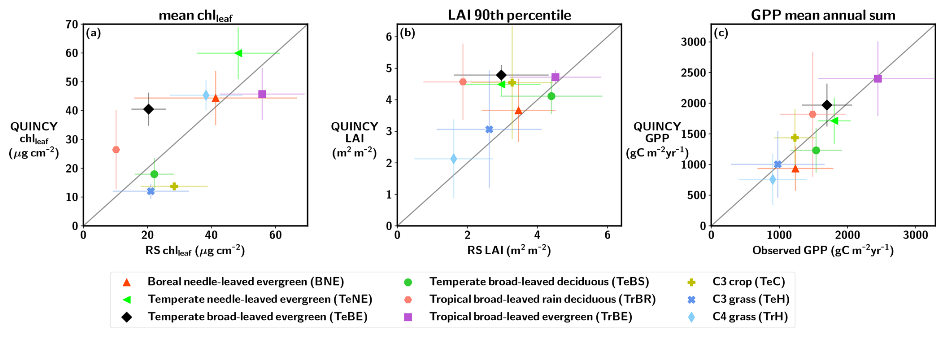
Figure 1 The PFT mean (a) chl_leaf, (b) LAI, and (c) GPP for the PLUMBER2 sites. The standard deviation is represented by whisker lines. A 1:1 line is marked with a gray line.

As expected, the within PFT variability between sites reveals greater scatter, the nature of which differs for chl_leaf and LAI (Figs. S2 and S3). For chl_leaf in all cases apart from TeBS, tropical broad-leaved evergreen forest (TrBE) and C4 grasslands (TrH), there is a lack of variation in the QUINCY chl_leaf, which present more constant values and smaller dynamic range compared to RS chl_leaf values (Fig. S2 and Tables S7 and S8). This is particularly pronounced for TeC and TeH sites, which give a range of 10–17 µg cm⁻² for TeC and 4–17 µg cm⁻² for TeH, for QUINCY and a range of 13–46 and 2–47 µg cm⁻² for RS, respectively. The site-level LAI estimates by contrast generally present a larger dynamic range (with the exception of TeBS, TeNE, TeBE and TrBE). The TrH in particular show a large overestimation in QUINCY LAI compared to RS LAI at higher LAI values (LAI>2.5) (Fig. S3).

The site-level GPP results show a good correlation between QUINCY estimates and eddy-covariance observations across PFTs. Whilst the correlation is generally along the 1:1 line, in 58 % of the PLUMBER2 sites, QUINCY underestimates the GPP on average by about 400 $\mathrm{g}\mathrm{C}{\mathrm{m}}^{-\mathrm{2}}{\mathrm{yr}}^{-\mathrm{1}}$. The majority of these underestimations are for BNE and TeBS forests. The QUINCY overestimation of GPP is mainly for crops and grasslands, with an average overestimation of 384 $\mathrm{g}\mathrm{C}{\mathrm{m}}^{-\mathrm{2}}{\mathrm{yr}}^{-\mathrm{1}}$ across 42 % of the PLUMBER2 sites. For the PLUMBER2 sites, the slight LAI overestimation of the TrH sites does not seem to lead to an overestimation of the mean GPP, but the QUINCY PFT mean GPP (756 $\mathrm{g}\mathrm{C}{\mathrm{m}}^{-\mathrm{2}}{\mathrm{yr}}^{-\mathrm{1}}$) is lower than the PFT mean of the observations (902 $\mathrm{g}\mathrm{C}{\mathrm{m}}^{-\mathrm{2}}{\mathrm{yr}}^{-\mathrm{1}}$). Due to very high LAI values for the GLOBAL TrH sites, the QUINCY mean GPP for the GLOBAL TrH sites was 1461 $\mathrm{g}\mathrm{C}{\mathrm{m}}^{-\mathrm{2}}{\mathrm{yr}}^{-\mathrm{1}}$ (not shown), and QUINCY chl_leaf mean was 50.2 µg cm⁻².

The QUINCY over- or underestimation in chl_leaf did not have a strong, detectable geographical pattern when assessed together and separately for all PFTs. The residual chl_leaf, i.e. the difference between the mean QUINCY and RS values, is shown in Fig. S5 in the Supplement on a map showing the geographical location of each site. For the C3 grassland sites, the QUINCY mean chl_leaf was rather small compared to the RS chl_leaf. When analyzing the residuals for the C3 grasslands, the northernmost sites seem to have less negative residuals in magnitude than for the sites around latitudes 30–60° N. This was also the case when the relative residual was analyzed (not shown). The greater QUINCY underestimation of chl_leaf for the warmer, southern C3 grassland sites is not related to the GPP underestimation. Interestingly, for the GLOBAL C3 grassland sites the LAI over/underestimation shows an opposite pattern to QUINCY chl_leaf: the northern sites show more negative LAI residual, and sites around latitudes 30–60° N mostly QUINCY overestimation of LAI (not shown), which could be due to the fact that RS chl_leaf is calculated using RS LAI.

The mean IAV of RS chl_leaf over all PFTs is 4.11±3.18 µg cm⁻², which is much higher than the corresponding value for QUINCY (1.35±1.52 µg cm⁻²). The RS chl_leaf IAV is higher for all other PFTs except for TrH, where the QUINCY chl_leaf IAV was 3.39±2.04 µg cm⁻², and the RS chl_leaf IAV was 3.37±2.35 µg cm⁻². The largest differences in IAVs between RS and QUINCY were seen for the evergreen sites. For example, the RS chl_leaf IAV for the BNE sites is $\mathrm{5.95}\pm \mathrm{3.51},$ and the QUINCY chl_leaf IAV is 0.5±0.4 µg cm⁻².

3.1.2 Seasonal cycle

The annual cycle of chl_leaf for the PLUMBER2 NH TeBS sites (Fig. 2) is similar when comparing QUINCY and RS. However, the start of the growing season is delayed in QUINCY. The SOS, EOS and LOS values for the PFT-averaged PLUMBER2 NH TeBS sites are presented in Table S9 in the Supplement. The QUINCY SOS for LAI is approximately 13 d later in spring compared to the RS LAI. Similarly, the end of the growing season is delayed in QUINCY, and the EOS of QUINCY chl_leaf occurs approximately 10 d later than in RS chl_leaf. While the RS LAI shows a decrease throughout the autumn season, QUINCY LAI remains at a high value until day of year (DOY) 280, which corresponds to mid-October. The EOS for QUINCY LAI is approximately 30 d later than for RS LAI. However, senescence occurs more rapidly in QUINCY than in the observations.

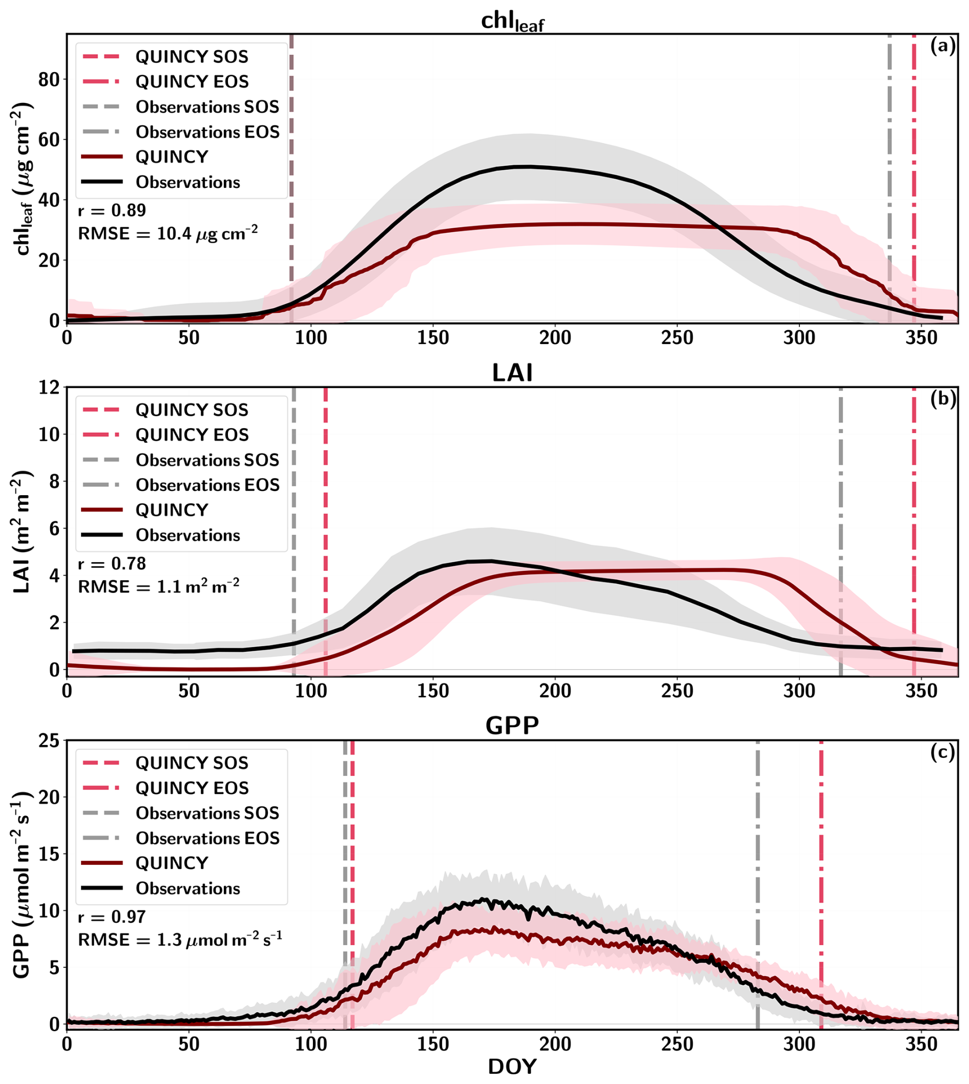
Figure 2 The average annual cycle of (a) chl_leaf, (b) LAI, and (c) GPP for the PLUMBER2 TeBS NH sites, as a function of the day of year (DOY). The shaded regions represent the standard deviation between sites. The start of season (SOS) and end of season (EOS) are marked with red (QUINCY) and grey (observations) vertical lines. The Pearson correlation (r) and root mean squared error (RMSE) are marked for each variable.

Figure 2c shows that the GPP between DOY 90–150 for QUINCY is slightly lower than in the observations. The spring development of GPP is slower in QUINCY than in the observations, though the QUINCY SOS of GPP occurs almost at the same time as in the measurements. Although the simulated LAI remains at the summer level until DOY ∼280, the simulated GPP decreases due to the environmental conditions in autumn. However, the delay in autumn LAI senescence is reflected in the QUINCY GPP EOS, which is approximately 26 d later than for the GPP observations. The delay in the QUINCY spring GPP is compensated partly for by the delayed end of the season where the QUINCY GPP is higher than the observed GPP after DOY 275. The mean GPP 3 month sum for the PLUMBER2 NH TeBS sites for spring (March, April and May, MAM) is 289 g C m⁻² for the observations, while for QUINCY, the value is 196 g C m⁻². The corresponding 3 month sum values for autumn (September, October, November, SON) for observations is 256, and 351 g C m⁻² for QUINCY.

Figures S6 and S7 in the Supplement show the PFT-mean seasonal cycles of chl_leaf and LAI for the PLUMBER2 and GLOBAL NH sites, and Fig. S8 in the Supplement for GPP for the PLUMBER2 NH sites. The most visible difference between QUINCY and RS chl_leaf and LAI seasonality can be observed for the boreal and temperate evergreen sites (Figs. S6a, c, and f and S7a, c, and f): QUINCY shows very little variation across seasons, while the RS indicates more variation throughout the year with a clear seasonal cycle. Nevertheless, the QUINCY GPP for these PFTs (Fig. S8a, b, and e) shows a similar annual cycle as the eddy covariance observations, and the correlation r for the evergreen needle-leaved sites is high (r>0.95). For the boreal needle-leaved deciduous forest (BNS) sites (Figs. S6b and S7b), the biases in seasonal cycle were similar to the TeBS results (Figs. S6d and S7d).

QUINCY chl_leaf for TeH and TeC sites show a delay in spring compared to RS chl_leaf, but this was not observed for QUINCY LAI. In autumn, the decrease in QUINCY chl_leaf and LAI occur later than in RS. For the TrH sites (Fig. S6j), the seasonal cycle of QUINCY chl_leaf and LAI differ from the observed seasonal cycle. The lowest PFT mean chl_leaf for QUINCY is in April (DOY∼100). Of the 47 TrH sites in the NH, 74 % of the sites had a higher QUINCY winter (December, January, February, DJF) chl_leaf average compared to the QUINCY spring (March, April, May, MAM) chl_leaf mean. Furthermore, 55 % of the TrH NH sites were such that the QUINCY DJF means of both chl_leaf and LAI were higher than the QUINCY MAM means. RS chl_leaf shows (Fig. S6j) the largest TrH averages for summer (June, July, August, JJA) and September, and a fairly clear seasonal cycle.

3.1.3 In-situ comparison of chl_leaf for two needle-leaved forests

The seasonal cycle of chl_leaf, LAI, fAPAR and GPP for Sodankylä is shown in Fig. 3, and the chl_leaf values of the US-NR1 site are presented in Fig. S9 in the Supplement. The mean annual and seasonal chl_leaf and GPP values are presented in Table S10 in the Supplement.

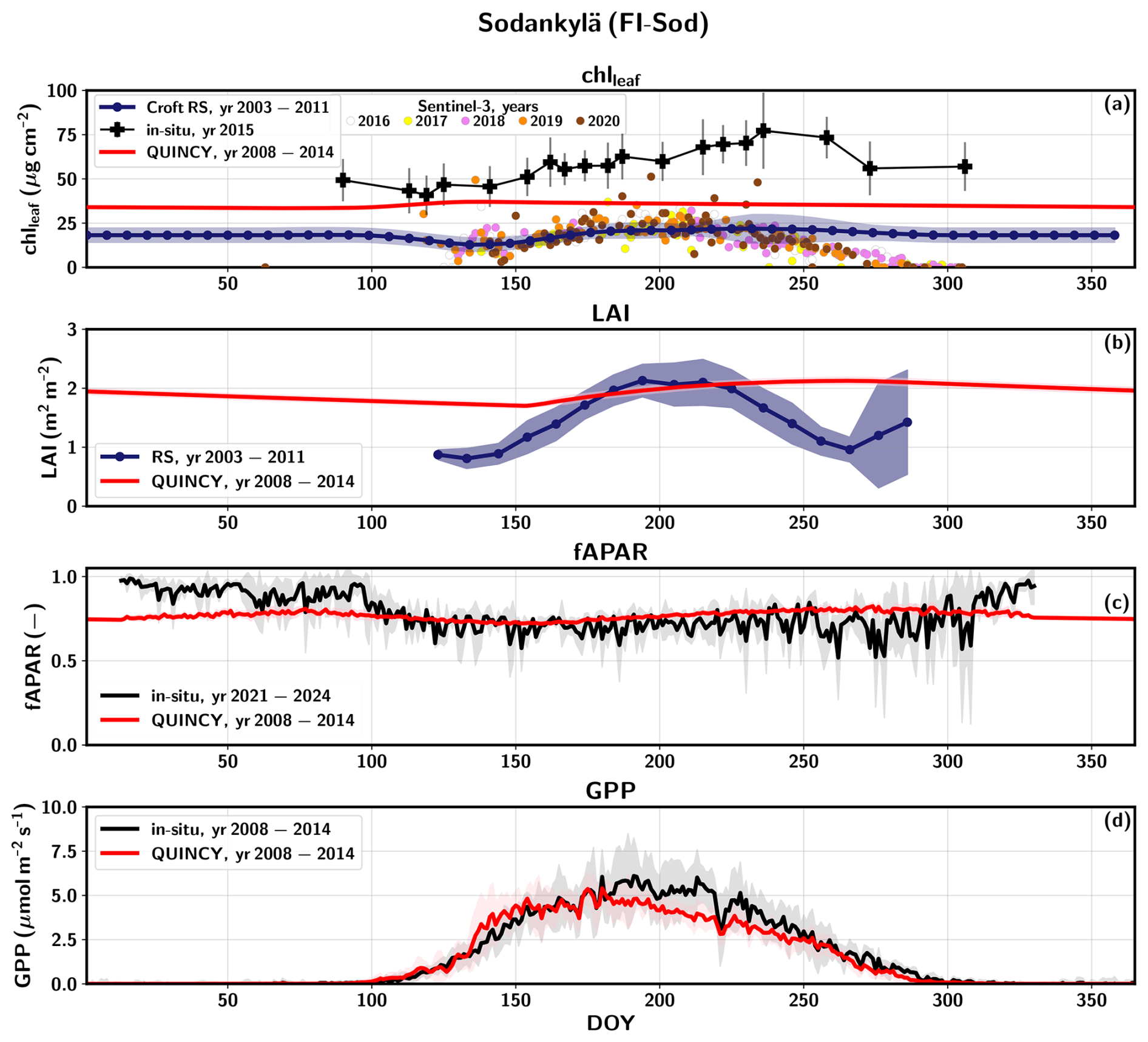
Figure 3 Seasonal cycle of daily means for FI-Sod (a) chl_leaf, (b) LAI, (c) fAPAR, and (d) GPP for QUINCY, remote sensing (RS) and in-situ measurements. The standard deviation for some of the data series is visualized as a shaded area. The Sentinel-3 chl_leaf values for different years are shown with different colors (2016 = white, 2017 = yellow, 2018 = pink, 2019 = orange, 2020 = brown).

Figure 3a highlights that the QUINCY chl_leaf values are in a range comparable to the in-situ observations for FI-Sod, but the QUINCY mean (Table S10) is lower than the annual mean of the in-situ measurements. On the contrary, the RS chl_leaf by Croft et al. (2020) shows much lower values. In addition, the mean of the Sentinel-3 RS chl_leaf is also lower than the in-situ or QUINCY chl_leaf but close to the mean RS chl_leaf by Croft et al. (2020).

The RS LAI in Fig. 3b shows a clear seasonal pattern for FI-Sod, which has a small effect on the RS chl_leaf. The summer (JJA) average RS chl_leaf is approximately 10 % higher than the winter (DJF) average, which is a relatively small difference compared to the interannual variability (∼4 µg cm⁻²). In addition, the late spring RS chl_leaf between DOY 100–151 show lower values than winter or summer. The late spring RS chl_leaf averages 14.6 µg cm⁻², approximately 27 % less than the JJA average. Similar spring decreases in RS chl_leaf were also observed for other BNE sites. The Sentinel-3 chl_leaf peaks in midsummer, and also shows a clear seasonal pattern. The in-situ chl_leaf is slightly higher in late summer (DOY 200–240) compared to spring and fall.

QUINCY LAI shows a small seasonal variation, which is reflected in the simulated chl_leaf. The winter QUINCY average is slightly lower than the summer QUINCY average chl_leaf. The in-situ fAPAR values are in agreement with the simulations during most of the year, but show a stronger seasonal variation than the QUINCY fAPAR (Fig. 3c), with higher values during winter.

QUINCY GPP is in line with the observations until DOY 175, but then decreases until the end of the season (Fig. 3d). However, the difference in annual GPP is not large, and annual QUINCY GPP is on average approximately 9 % lower than the in-situ GPP. The difference between observed and simulated GPP after DOY 175 could be due to missing late fall chl_leaf development or due to too strong response to a drought.

The mean in-situ chl_leaf for the US-NR1 site was close to the QUINCY chl_leaf mean (Fig. S9 and Table S10). The minimum value of individual tree samples was 26.8 µg cm⁻² and the maximum was 60.8 µg cm⁻², i.e. there was variation between individual samples that is partially minimized by the averaging. The in-situ observations show a slight increase during spring, but the variation is large due to the small number of samples. The mean in-situ chl_leaf for DOY 1–150 is 37.1±6.1 µg cm⁻², while the mean for summertime is 43.2±2.3 µg cm⁻². The summer QUINCY chl_leaf was close to the annual mean, i.e. there was no pronounced seasonal cycle. The RS chl_leaf annual mean by Croft et al. (2020) was lower than the annual mean chl_leaf of in-situ measurements or QUINCY. Interestingly, the RS chl_leaf shows a lower JJA mean than the annual mean. Similarly to the FI-Sod RS chl_leaf, there is a decrease in the spring chl_leaf after DOY 100, and the decrease is more pronounced than for Sodankylä. The minimum value (∼16 µg cm⁻²) of RS chl_leaf averaged annual cycle appears around DOY 155, with an increase after that. For the Sentinel-3 chl_leaf, the mean chl_leaf was close to the QUINCY values, although the numerical range was much wider. The JJA mean for Sentinel-3 is close to the in-situ observations, and approximately 32 % higher than the QUINCY JJA chl_leaf. The annual QUINCY GPP was 45 % lower than the observed GPP. In addition, the QUINCY JJA LAI (not shown) was 2.2±0.1 m² m⁻², and was lower than the RS JJA LAI (2.5±0.2 m² m⁻²), which may partially explain the underestimation of GPP. Bowling et al. (2018) report that the observed in-situ LAI at the site is 3.8–4.2 m² m⁻².

3.2 Nitrogen limitations in QUINCY

Figures 4a–c show the QUINCY leaf C:N ratios and the corresponding QUINCY chl_leaf values for three PFTs. The TeBS sites show an almost linear relationship between chl_leaf and leaf C:N with a correlation of $r=-\mathrm{0.87}$ ($p<\mathrm{1}\times {\mathrm{10}}^{-\mathrm{13}}$). Higher leaf C:N values indicate lower leaf N levels relative to leaf C. This leads to lower chl_leaf since chl_leaf is a function of leaf N. The same nearly linear relationship between QUINCY leaf C:N and decreasing chl_leaf is seen for the BNE sites (Fig. 4c) with a correlation of $r=-\mathrm{0.96}$ ($p<\mathrm{1}\times {\mathrm{10}}^{-\mathrm{40}}$). The TeH sites represent a more scattered pattern and the correlation is only $r=-\mathrm{0.58}$ ($p<\mathrm{1}\times {\mathrm{10}}^{-\mathrm{9}}$), indicating that chl_leaf is more influenced by other factors, such as water availability, temperature and precipitation than leaf C:N levels, compared to BNE and TeBS. However, for the TeH sites, both the QUINCY chl_leaf and leaf C:N values are in a narrower range compared to the other two PFTs, which partly affects the comparison.

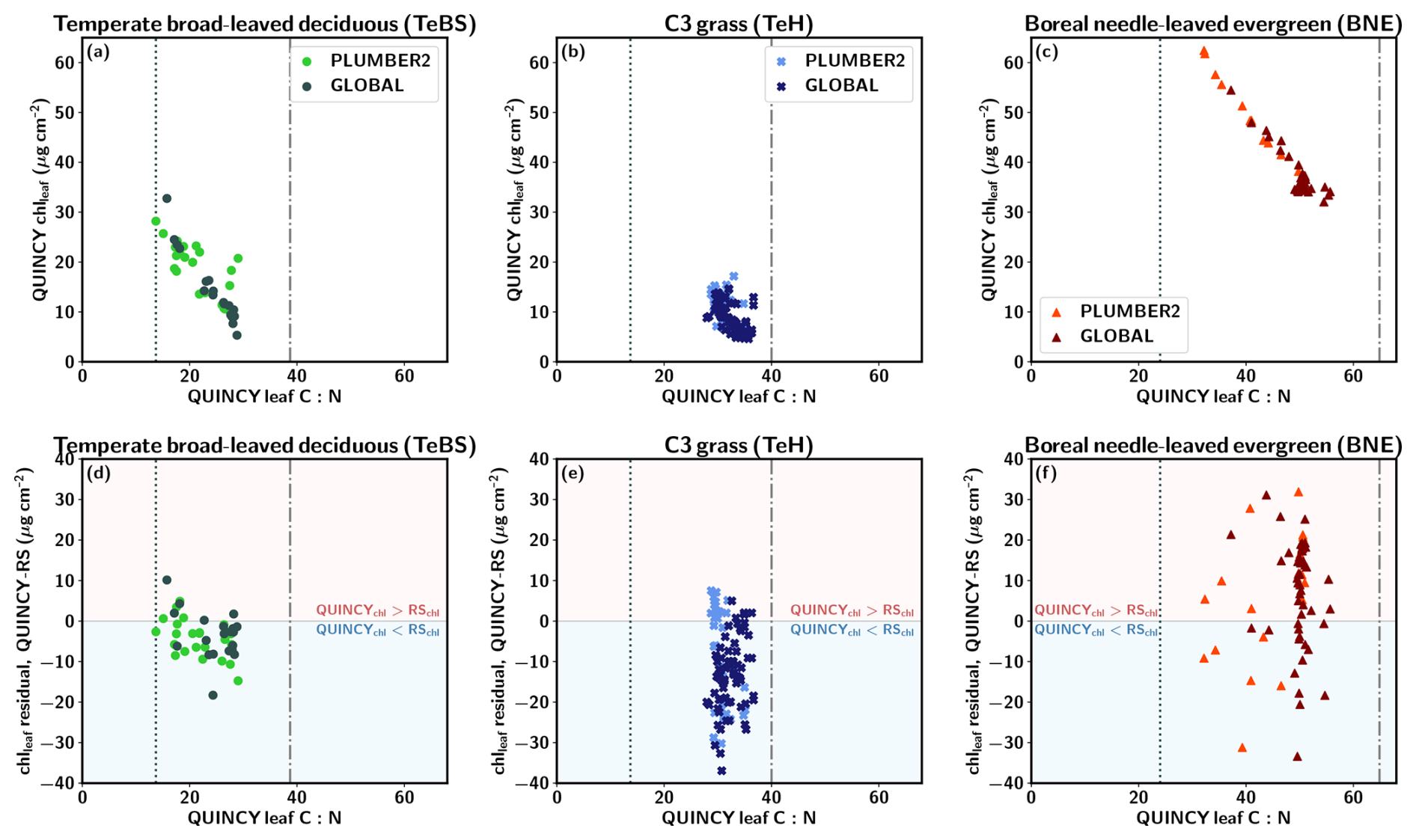
Figure 4 QUINCY leaf C:N and chl_leaf and the corresponding residual for (a, d) temperate broad-leaved deciduous (TeBS), (b, e) C3 grassland (TeH), and (c, f) boreal needle-leaved sites (BNE). The vertical lines show the QUINCY leaf C:N minimum and maximum limits.

For the TeBS sites, the chl_leaf residual is moderately connected to QUINCY leaf C:N values (Fig. 4d), but the same is not true for the BNE and TeH sites. Especially for the PLUMBER2 TeBS sites, the chl_leaf residual is more negative for the sites with higher leaf C:N values. The TeH sites do not show much variation in the leaf C:N values, and the chl_leaf residual does not appear to be connected to the magnitude of leaf C:N. The 90th percentile of TeH leaf C:N is 35.0, which is 88 % of the QUINCY maximum leaf C:N. The BNE 90th percentile leaf C:N is 51.1 (78 % of the maximum) and the TeBS 90th percentile leaf C:N is 28.1 (73 % of the maximum value).

The majority of the GLOBAL BNE sites are clustered in a region with mean QUINCY chl_leaf around 35–40 µg cm⁻² and leaf C:N ratio around 50. The GLOBAL set contains more BNE sites at higher latitudes than the PLUMBER2 set (see Fig. S1). In addition, most (over 83 %) of the PLUMBER2 and GLOBAL sites with leaf C:N ∼50 are in a region with a mean annual temperature below 5 °C. The median chl_leaf residual for the GLOBAL and PLUMBER2 sites is 9.9 µg cm⁻² and 7.4 µg cm⁻², respectively.

We analyzed whether the chl_leaf residual is connected to the GPP residual, i.e. the difference between QUINCY annual GPP and observed annual GPP (not shown). For the PLUMBER2 TeBS sites, the largest negative GPP residual, i.e. the model underestimated GPP, was for those sites that are more N-limited in QUINCY and have a negative chl_leaf residual. For the PLUMBER2 TeH sites, the GPP residual was weakly negatively correlated with the chl_leaf residual: the largest positive GPP residual is observed for the sites that have strong negative chl_leaf residual. Similarly, the GPP residual for the PLUMBER2 BNE sites was not strongly connected with the chl_leaf residual.

We also compared the QUINCY leaf C:N ratios with in-situ measured values for two sites (FI-Hyy and US-MMS) obtained from the TRY database. This was done to assess whether the QUINCY leaf C:N values are at a realistic level for individual sites. US-MMS is classified as a TeBS site and FI-Hyy is classified as a BNE site. For the US-MMS site, the QUINCY average leaf C:N was 17.3, and the TRY database average was 21.3. The US-MMS QUINCY leaf C:N is close to the lower leaf C:N threshold, and the QUINCY chl_leaf is underestimated by 27 % compared to RS chl_leaf. For the FI-Hyy site, the values were 46.5 and 38.8, respectively. The QUINCY chl_leaf was underestimated by 28 %, which indicates that for FI-Hyy, there is a slightly too strong N-deficit modelled.

In order to study the effects of N limitation, we briefly analyzed the QUINCY C_only simulation results for the PLUMBER2 BNE sites (not shown). The results revealed that at low chl_leaf values, the difference between GPP from QUINCY default, i.e. CN, and C_only simulations was greater than at higher chl_leaf levels for the BNE. In addition, for the sites where the N deposition was low, the chl_leaf values were also small.

3.3 Leaf N allocation schemes

Figure 5 shows that the alternative, more realistic N allocation scheme leads, on average, to greater chl_leaf and GPP underestimation for the TeBS sites compared to the QUINCY default. Furthermore, the alternative N allocation scheme produces lower leaf chl_leaf (14.9±4.4 µg cm⁻²) than the QUINCY default (17.9±5.6 µg cm⁻²) for the PLUMBER2 TeBS sites (Fig. S10 and Table S11 in the Supplement). The corresponding RS chl_leaf mean is 22.1±6.1 µg cm⁻². Similarly, the TeBS mean GPP is lower for the alternative N fraction scheme, 1044±311 $\mathrm{g}\mathrm{C}{\mathrm{m}}^{-\mathrm{2}}{\mathrm{yr}}^{-\mathrm{1}}$, while the QUINCY default mean GPP is 1231±366 $\mathrm{g}\mathrm{C}{\mathrm{m}}^{-\mathrm{2}}{\mathrm{yr}}^{-\mathrm{1}}$. For the observations, the mean GPP is 1539±377 $\mathrm{g}\mathrm{C}{\mathrm{m}}^{-\mathrm{2}}{\mathrm{yr}}^{-\mathrm{1}}$. The LAI 90th percentile values are in a similar range ($\sim \mathrm{4}\pm \mathrm{1}$ m² m⁻²) between the QUINCY default simulation and QUINCY alternative N allocation. The underestimation of GPP and chl_leaf is most likely due to lower f_N,rub. While the summer (JJA) f_N,rub for the QUINCY default is on average 0.20 for the PLUMBER2 TeBS sites, the corresponding average for the alternative N allocation scheme is 0.09.

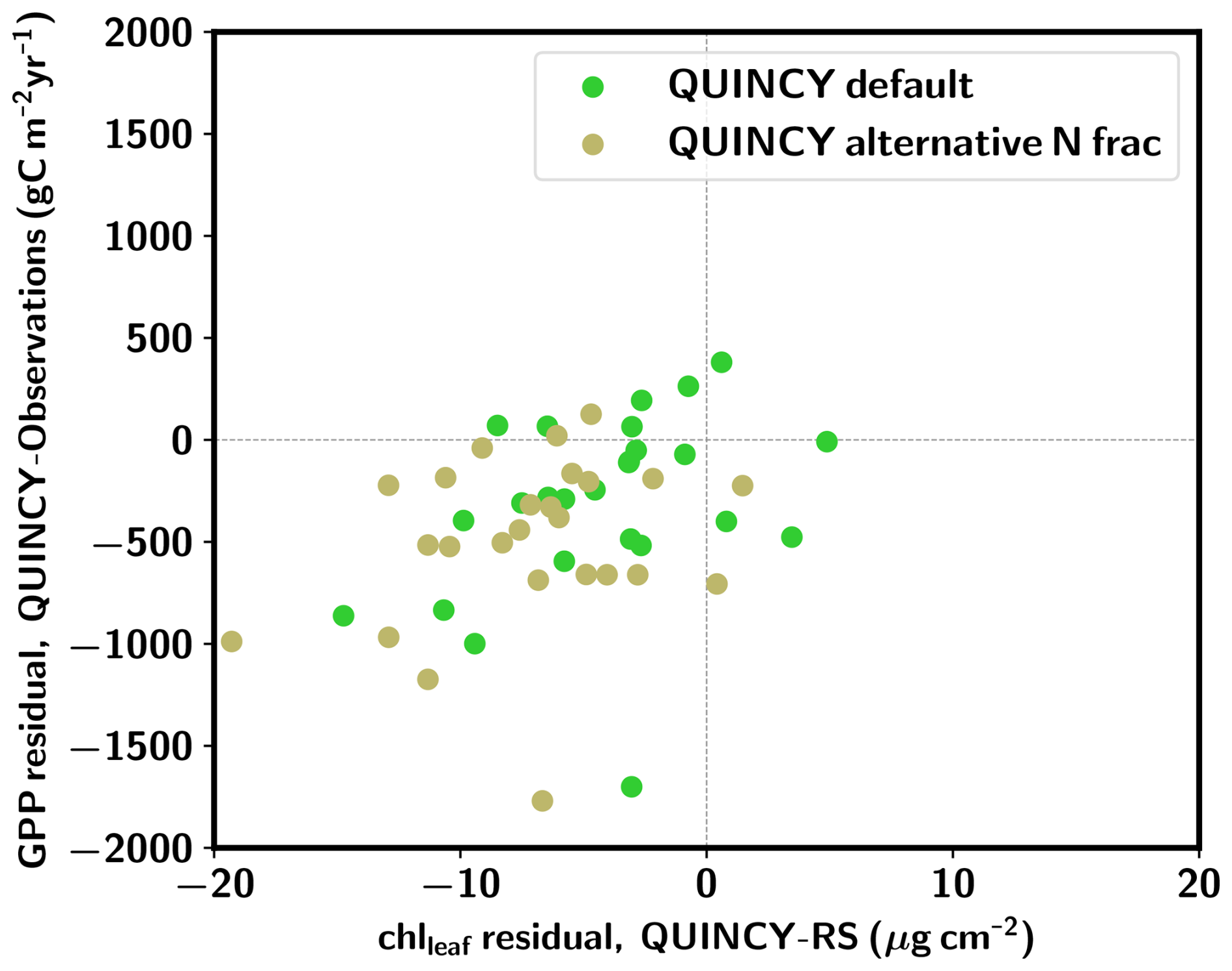
Figure 5 GPP residual (QUINCY – observations) vs. chl_leaf residual (QUINCY – observations) for the PLUMBER2 TeBS sites. The QUINCY default scheme results are marked with green circles, and QUINCY alternative N fraction results are marked with beige circles.

The results for the other PFTs were similar to those for TeBS: the chl_leaf and GPP magnitudes were lower with the alternative N allocation scheme (Table S11). An exception is the TrH sites, where the annual GPP was higher with the alternative N allocation than with the default QUINCY scheme. This was due to increased proportions of leaf N in Rubisco and electron transport, while f_N,chl was decreased and the f_N,struct slightly increased. The PFT mean values for f_N,struct and other fractions were calculated over sites globally, i.e. including the Southern Hemisphere sites. This affects the comparison slightly, as the seasonal cycles differ between the Northern and Southern Hemispheres.

Increasing chl_leaf affects more the QUINCY default chl_leaf levels than QUINCY alternative N fraction output, but the difference is not large (Table S12 in the Supplement). When f_N,chl is increased in QUINCY default, the mean chl_leaf increases by 37.4 %, while the mean LAI 90th percentile decreases by 2.4 % and the mean annual GPP decreases by 6.3 %. This is due to the fact that in the QUINCY default, increasing f_N,chl decreases leaf N allocated in electron transport and Rubisco, since their fractions of leaf N are calculated after f_N,chl (see Sect. 2.4.1). For the alternative N fraction simulations, increasing f_N,rub which leads to increase in f_N,chl results in different dynamics compared to the QUINCY default scheme. In the alternative N allocation scheme, increasing f_N,rub resulted in an almost linear response in the chl_leaf magnitude, with an increase of 24.2 %. The increases in LAI and GPP were more moderate: 5.3 % and 12.1 %, respectively. In the QUINCY default simulation, increasing f_N,chl resulted in decreased GPP, while in the alternative N allocation scheme, GPP increased. Furthermore, the fraction in the structural part f_N,struct decreases in the alternative N allocation scheme when the f_N,rub and, consequently, f_N,chl are increased. In the default QUINCY simulation, increasing f_N,chl does not directly affect f_N,struct, but rather indirectly through its influence on leaf N, resulting in only a minor decrease of f_N,struct.

3.4 The environmental drivers of chl_leaf

Figures 6 and S11 in the Supplement show that when the RF fitting is done over all PFTs, the feature importances are very similar between QUINCY and RS. Air temperature has the largest impact on the random forest fitting of both QUINCY chl_leaf and RS chl_leaf, when the fitting is done using data from all PFTs. The effect of air temperature is even larger for the TeH and TeBS sites compared to the importance calculated over all PFTs. This result is logical, since chl_leaf is formed from leaf N, which is partly dependent on temperature via soil N mineralisation and biological nitrogen fixation (BNF). The QUINCY BNE sites do not show such a strong dependence on air temperature because the evergreen needle chl_leaf does not vary as much throughout the year as deciduous chl_leaf. However, temperature shows a permutation importance of 0.26±0.003 for QUINCY BNE, which is most likely a result of different sites being in different temperature regimes.

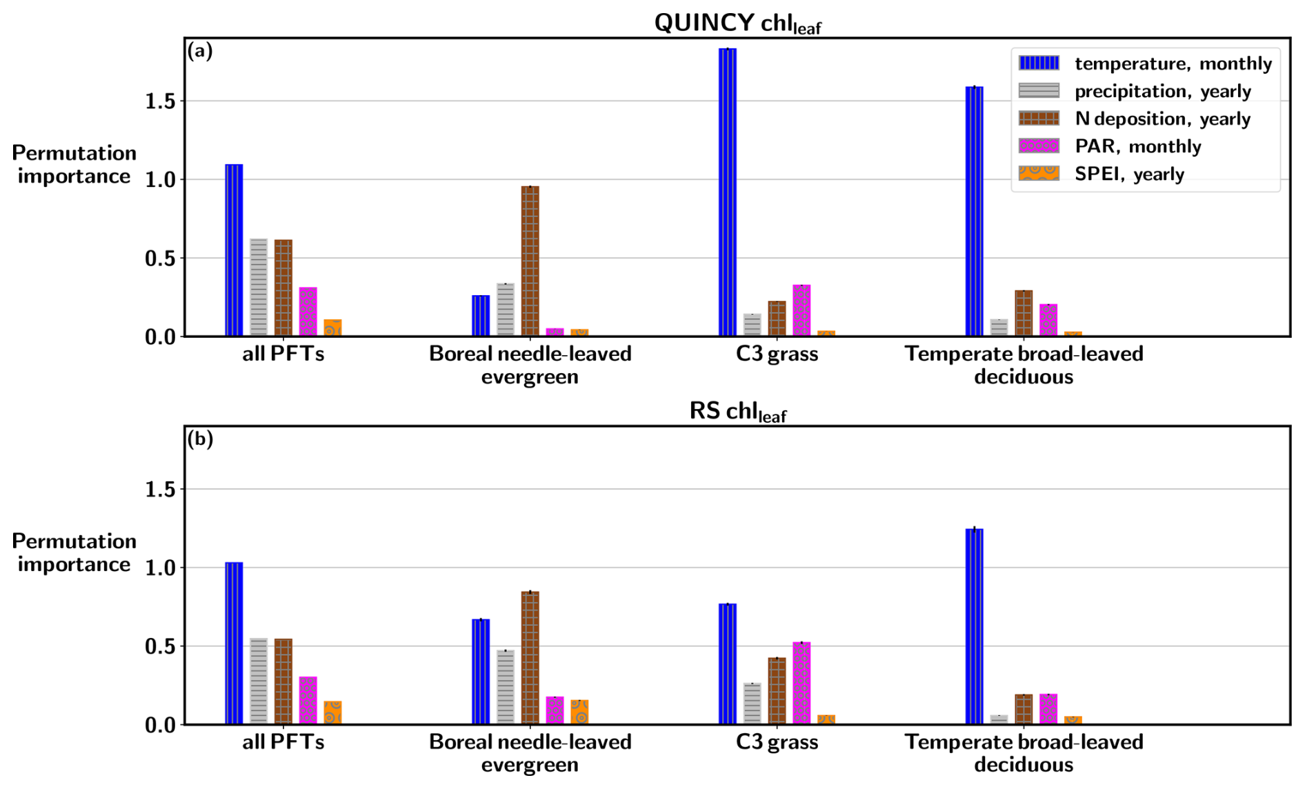
Figure 6 Permutation importance values based on random forest regression fitting for (a) QUINCY chl_leaf and (b) RS chl_leaf, based on data from all sites, and separately for BNE, TeH, and TeBS sites.

Figure S11 shows that nitrogen deposition is the most dominant driver for evergreen ecosystems for QUINCY chl_leaf. For the BNE and TeNE sites, the permutation importance values are 0.95±0.007 and $\mathrm{1.78}\pm \mathrm{0.054},$ respectively, and the contribution of other environmental drivers is smaller. For the RS chl_leaf of BNE sites, N deposition has the highest permutation importance value (0.84±0.012), but the role of N deposition in the RS observations is not as pronounced compared to other variables as in QUINCY. The RS chl_leaf for the TeNE sites is largely driven by temperature (permutation importance $=\mathrm{0.63}\pm \mathrm{0.043}$). The grasslands (TeH and TrH) show similar contributions from different variables for QUINCY and RS, although RS chl_leaf is less affected by temperature than QUINCY. There is a difference in the permutation importances for the TeC sites between QUINCY and RS, as QUINCY chl_leaf is more influenced by temperature and RS chl_leaf indicates a slightly mixed effect of different environmental drivers.

The results of the SHAP analysis (Figs. S12 and S13 in the Supplement) are similar to the permutation importance calculations: air temperature is a dominant driver for both QUINCY and RS. In addition, the SHAP values indicate that warmer temperatures lead to higher than average chl_leaf values, and colder temperatures lead to lower than average chl_leaf values. The SHAP analysis for QUINCY chl_leaf suggests that the higher PAR values lead to lower chl_leaf values, although the majority of the data points are close to SHAP values of zero, i.e. PAR is not a strong driver of chl_leaf compared to, for example, temperature. For the RS chl_leaf, a similar pattern is not found, but the higher PAR would have an increasing effect on chl_leaf.

4 Discussion

4.1 QUINCY's ability to reproduce chl_leaf, LAI and GPP magnitudes

4.1.1 Magnitude of chl_leaf

When analyzed across all sites, QUINCY chl_leaf correlated well with RS observations and the PFT specific values were generally in line with the observations, and the simulated PFT-mean values were similar to RS chl_leaf. In particular, the PFT mean chl_leaf of the BNE and TeBS sites was close to the mean RS observations of these PFTs. However, QUINCY generally produced lower variability in chl_leaf between sites compared to RS. Particularly for C3 grasslands and crops, the QUINCY chl_leaf was restricted to too narrow a range compared to RS observations. This suggests that QUINCY lacks some processes that cause variation in RS chl_leaf values, and that the QUINCY dynamics for C3 grasses and crops require further in-depth analysis to explain the missing variation. In addition, the chl_leaf QUINCY parameterization for C3 grasslands is the same as for trees, which could affect chl_leaf dynamics. Fertilization and other management practices are not included in the version of QUINCY used in this study, which could explain the difference in the chl_leaf numerical ranges between QUINCY and RS. This may affect the comparison of magnitude and seasonality for C3 cropland sites. Lu et al. (2020) gathered a collection of different chl_leaf in-situ observations distributed globally. When comparing the QUINCY chl_leaf values with those reported by Lu et al. (2020), it was observed that C3 crops and C3 grasslands are most likely underestimated, similarly when compared to the RS chl_leaf values. The correlation between QUINCY chl_leaf and RS chl_leaf was poor for C3 grasslands and C3 crops. This also highlights the need for tuning the QUINCY parameterization for grasslands, and possibly other changes to the model structure to capture the grassland chl_leaf dynamics.

Some of the PLUMBER2 sites are located in fens and wetlands, and these are classified as C3 grasslands in QUINCY. The model version of QUINCY used in this study does not include wetlands or fens, and therefore for some of the sites (e.g. FI-Lom in high latitude region) QUINCY does not model the relevant water table depth dynamics, which may influence the carbon and water dynamics at the sites.

For C4 plants, the range for QUINCY values was similar to RS chl_leaf for higher values, but lower chl_leaf concentrations were missing in QUINCY. Lu et al. (2020) reported 15–60 µg cm⁻², while the QUINCY chl_leaf range for C4 grasslands was 31–72 µg cm⁻². The RS chl_leaf range for C4 grasslands was 12–63 µg cm⁻². However, it should be noted that QUINCY chl_leaf values only represent the top of the canopy, while in-situ observations may have mixed results from different canopy heights, which may affect the comparison.

For the BNE sites, the QUINCY chl_leaf overestimation was higher for GLOBAL than PLUMBER sites, and relatively higher portion of GLOBAL BNE sites were located in high latitudes. This suggests that the QUINCY chl_leaf overestimation or RS chl_leaf underestimation, is more pronounced for the needle-leaved sites in cold regions, which could partly reflect the challenges of optical remote sensing in high latitudes.

Our machine learning-based analysis indicated that QUINCY is able to capture the influence of environmental drivers of the chl_leaf in a big picture. QUINCY chl_leaf for evergreen sites was driven by N deposition, with other environmental variables contributing less. The same was true for the RS chl_leaf for BNE and TrBE but not for TeNE. Additional comparison of QUINCY simulations with active C and N cycles with a C_only simulation also demonstrated a similar conclusion. Though, the RS chl_leaf for BNE sites seemed to be more temperature-driven than for QUINCY. This could be explained by differences in the seasonal cycle, as RS chl_leaf shows a seasonal pattern for BNE sites, while QUINCY does not. In addition, it was observed that QUINCY chl_leaf for the TeC sites was mainly driven by temperature, while RS chl_leaf had more equal contributions from different variables. In addition, the footprint size of RS chl_leaf may affect the comparison, as crops are typically located in a heterogeneous landscape. The analysis with the SHAP values revealed that higher PAR values could produce lower chl_leaf in QUINCY simulations. The decreasing effect of higher PAR values on QUINCY chl_leaf could be partly due to the tropical regions, where the PAR radiation does not vary as much throughout the year. The decreasing effect could be also attributed to differences between different sites.

4.1.2 Magnitudes of LAI and GPP

The QUINCY annual GPP showed a good correlation with PLUMBER2 observations, however, the values were underestimated at most of the sites. This could be partly due to a slightly delayed growing season for the deciduous forests (Fig. S8), which hinders the early spring carbon sequestration. The delayed seasonal development calls for tuning the QUINCY phenology parameters, which could benefit the simulations with a reasonable amount of work. However, for some of the PFTs (TeC, TrBR, TeBE), QUINCY overestimated GPP.

The simulated LAI over all PFTs was generally in an agreement with RS LAI (Fig. S3d and Table S8). However, a clear future development point for QUINCY is the overestimation of LAI values, which was the case for most of the PFTs. The overestimation of LAI in QUINCY could be due to, for instance, missing herbivores and management. These effects are currently under development in QUINCY. The overestimation of LAI is pronounced for the C4 grasslands, for which the LAI values in QUINCY were unrealistically high. The very high LAI values were observed for the GLOBAL sites located on the African and South American continents, for which we did not have GPP ground station data. However, the QUINCY GPP for the PLUMBER2 C4 grassland sites was within a reasonable range, and the QUINCY PFT mean GPP was close to the observed PFT mean GPP. This suggests that despite high LAI, QUINCY is able to account for environmental conditions affecting GPP and maintain realistic GPP levels. However, for the GLOBAL C4 grassland (TrH) sites, it was observed that if the simulated extremely high LAI values were coupled with high chl_leaf, this resulted in high simulated GPP values. The RS observations could potentially be used in model tuning to balance the overestimation of both LAI and chl_leaf.

Although QUINCY tended to overestimate LAI in general, for TeBS it was mostly underestimated. Similarly, the QUINCY mean chl_leaf is underestimated at the majority of the TeBS sites. However, when analyzing the residuals for individual sites, the GPP under- or overestimation was not always related to the chl_leaf or LAI residual. Less than half of the 25 PLUMBER2 TeBS sites showed an underestimation for all chl_leaf, LAI, and GPP. Overestimation of LAI can potentially lead to too strong shading, which could result in reduced GPP in lower canopy layers. The radiative transfer model might therefore play a role in the underestimated GPP.

4.2 QUINCY's ability to reproduce the observed seasonal cycle

The seasonality of GPP for QUINCY was consistent with the observations for many of the PFTs. However, the seasonality for chl_leaf and LAI in QUINCY was found to have differences compared to RS values for some of the PFTs.

The annual cycle of QUINCY chl_leaf for deciduous forest sites was similar when QUINCY and RS chl_leaf were compared. However, the increase in QUINCY chl_leaf in spring occurred late compared to RS chl_leaf, as well as decrease in autumn chl_leaf. The QUINCY LAI estimations showed similar biases when compared against RS results. However, this was not reflected as prominently in the seasonality of GPP compared to the delay in LAI, most likely due to environmental drivers. This indicates that QUINCY is able to maintain reasonable GPP levels in autumn even when LAI is overestimated. For the NH PLUMBER2 TeBS sites, the PFT-averaged seasonal cycle showed that the QUINCY underestimation of annual GPP is not too strongly affected by the delay in start of the growing season. The GPP sum for the spring (MAM) was underestimated by QUINCY by ∼93 g C m⁻², while the overestimation in the autumn (SON) was 95 g C m⁻², i.e. they compensate each other.

The QUINCY chl_leaf and LAI seasonality differed from RS observations for the boreal and temperate evergreen sites. QUINCY chl_leaf and LAI do not change as much from season to season at these evergreen sites, whereas RS chl_leaf and LAI show more variation during the year. The RS chl_leaf for BNE forests implied a stronger seasonal cycle than what was seen from in-situ observations at two BNE sites, which was most likely driven by too strong LAI seasonality of the RS product. In addition, the RS observations for the Sodankylä (FI-Sod) and Niwot Ridge (US-NR1) sites indicated a slight decrease in spring chl_leaf, and this was seen also for other BNE sites. The decrease in RS chl_leaf in spring could be driven by resorption of N to form new needles, or by the impact of the understory during the snow-melt season. A study by Zhang et al. (2019), conducted in a laboratory environment, demonstrated a similar decrease for a boreal evergreen forest. The RS chl_leaf retrieval algorithm does not consider variations in understory, and therefore the understory vegetation can cause artifacts to the retrieved needle-leaf reflectance signal. In addition, the mountainous landscape surrounding US-NR1 might affect RS retrieval, which also can create artifacts to the mean RS chl_leaf. The Sentinel-3 chl_leaf shows the strongest seasonal cycle at the US-NR1 site compared to other products used in this study, which could be partly due to assumptions made in the retrieval processing. For instance, the assumptions made for the LAI seasonality and the effect of snow cover can affect the RS chl_leaf retrieval. For temperate broad-leaved evergreen sites, QUINCY did not simulate seasonal variation in chl_leaf, while RS chl_leaf showed a clear increase in spring and decrease in fall. Site-level studies have indicated contradicting results for chl_leaf seasonal cycle for temperate evergreen forests (Joshi et al., 2024; Yasumura and Ishida, 2011), therefore it is not straightforward judge whether the model behavior is erroneous.

The in-situ observations in the boreal Sodankylä forest (Fig. 3a) for the year 2015 showed that the chl_leaf concentrations increased throughout the growing season in needle-leaved forests. Similar behavior at other evergreen needle-leaved forests was reported by Laitinen et al. (2000) and Katahata et al. (2007). The increase in chl_leaf could indicate that the Sodankylä forest may be N-limited, and requires strong N uptake throughout the summer. The observations from the Niwot Ridge forest did not show such a strong pattern (Fig. S9), as also shown by Bowling et al. (2018), potentially reflecting a different N status of the ecosystem.

For TeC and TeH sites, the seasonal cycle of QUINCY chl_leaf was delayed compared to RS, but the bias was not large. The lower QUINCY spring chl_leaf for NH TrH sites suggests that the phenological cycle for these sites needs further tuning in QUINCY, and is most likely linked to simulated LAI biases. In QUINCY, the start of senescence is controlled by soil moisture and temperature thresholds. Given the high species diversity in herbaceous systems, both within and between sites, ecosystem-level models such as QUINCY often struggle to capture phenological variation. This is partially due to PFT-level parameters not reflecting diversity at the site level, and partially due to the difficulty of capturing an average response of diverse species.

4.3 Modeling the N cycle and N limitation

QUINCY is one of the state-of-the art TBMs that include an advanced representation of chl_leaf in the canopy, and also the connection between chl_leaf and N limitation. This allows the intercomparison to remote sensing chl_leaf products, which can be further extended to cover analysing the N limitation on photosynthesis and the implications on carbon sequestration efficiency. In addition, our analysis demonstrated how to use chl_leaf as a metric to support analysing the N limitation in simulations. However, one needs to keep in mind that the modelled and remotely sensed chl_leaf are not completely equivalent, but there are conceptual differences in spatial coverage, for instance.

The strongest QUINCY GPP underestimation for the PLUMBER2 TeBS sites was connected to stronger N-limitation and QUINCY chl_leaf underestimation, suggesting a too strong modeled N limitation for these sites. However, the leaf C:N values were not close to the maximum leaf C:N values for the TeBS sites, suggesting that the QUINCY maximum threshold value of leaf C:N may be slightly too high (Fig. 4d). Though, we compared QUINCY leaf C:N values to the TRY database observation leaf C:N values for two sites, and the QUINCY values were in line with the observations.

Some of the QUINCY chl_leaf underestimation for the TeBS sites could be due to lower N availability or allocation to leaves (Fig. 4d). Both the QUINCY underestimation of chl_leaf and also GPP could be partly related to modeling deficiencies in the N cycle. The QUINCY mean symbiotic BNF was ∼0.3 $\mathrm{g}{\mathrm{Nm}}^{-\mathrm{2}}{\mathrm{yr}}^{-\mathrm{1}}$ for the TeBS sites. Davies-Barnard and Friedlingstein (2020) report that for deciduous broad-leaved forests, including both tropical and temperate forests, the mean symbiotic BNF is approximately 0.8 $\mathrm{g}{\mathrm{Nm}}^{-\mathrm{2}}{\mathrm{yr}}^{-\mathrm{1}}$, suggesting that QUINCY symbiotic BNF is underestimated for the TeBS sites. Though, the negative residual of chl_leaf between model and observations was higher with the higher leaf C:N values, indicating that QUINCY's modeled N deficit for the TeBS sites is too strong. The analysis shows that for the TeBS forests, the chl_leaf residual between simulated and RS chl_leaf brings additional information in pinpointing that the N-deficit influence is overestimated at certain sites and contributing to too low GPP.

For the BNE sites, QUINCY overestimated chl_leaf compared to RS chl_leaf, and the BNE chl_leaf and GPP residuals were not correlating, which may be partly be due to RS chl_leaf magnitude issues as presented in Sect. 3.1.3. The observed GPP increased as a function of observed chl_leaf (not shown), and this was also evident in the simulations. A comparison of QUINCY CN- and C-only simulations for the BNE sites indicated that QUINCY simulates an N deficit at low chl_leaf values, as GPP was lower with the CN-simulation. Including the N cycle in the simulations improved the model behavior and led to a decrease in simulated chl_leaf values at the lower end of the observations and improved model behavior in terms of chl_leaf and GPP. This shows a realistic behavior of the QUINCY N cycle. Furthermore, the low chl_leaf values coincided with the low N deposition values, indicating that N deposition plays a significant role in the N deficit of these ecosystems, as also shown in the feature importance analysis results.

In addition, the TeH leaf C:N values (Fig. 4e) were closer to the upper bound and covering only approximately half of the leaf C:N range derived from the TRY database, even when we had sites globally distributed across different climatological regions. This suggests that many of the TeH sites are more N-limited in QUINCY compared to BNE and TeBS sites, and that QUINCY has difficulty capturing TeH sites with high leaf N values. This may be a partial cause of the too low and also too static chl_leaf values for the TeH sites. For the TeH sites, QUINCY had the largest overestimation of GPP when the modeled chl_leaf is the most underestimated. This indicates that the leaf N allocation in QUINCY for TeH sites requires further parameter tuning. The QUINCY dynamics related to N cycling may require further analysis to estimate the contributions of N deposition and BNF to leaf N content, and to determine whether they are in the range of estimates presented in the reference literature.

Our analysis using the more advanced N allocation routine shows that the chl_leaf and GPP magnitudes for the TeBS sites were not improved compared to the observation data. This was partly due to lower f_N,rub. In the alternative N scheme, f_N,chl is a function of f_N,et and therefore a function of f_N,rub, and therefore the lower f_N,rub affects both GPP and chl_leaf. The underestimation of f_N,rub could be partly due to the LMA representation in QUINCY. LMA is the inverse of SLA, and thus it is the same fixed value per PFT, which may be too general a representation with respect to the N allocation scheme. On the other hand, the advanced N allocation scheme provided a more realistic mechanism when f_N,rub was increased by resulting in simultaneous increases in f_N,chl and GPP. This indicates that what the alternative N allocation scheme produces is more in line with the current ecophysiological understanding from the literature (Onoda et al., 2017; Evans and Clarke, 2019) regarding the relationship between V_c(max) and chl_leaf: increasing leaf N in chl_leaf does not decrease other photosynthetic fractions, but rather the structural part (f_N,struct).

4.4 Limitations of the analysis

4.4.1 Limitations due to remote sensing products

Although the satellite product by Croft et al. (2020) agrees well with the in-situ observations (Croft et al., 2020), the satellite retrieval products contain a certain degree of uncertainty. As Boegh et al. (2013) conclude, satellite inversions are often ill-posed inversion problems, which can complicate the retrieval of chl_leaf and LAI from remote sensing data. Furthermore, the coverage of the MERIS satellite data is not optimal for certain regions such as South America, the tropics, western Australia, and parts of the boreal zone. This is partly due to gaps in the original data caused by clouds, sensor errors, or light conditions (Tum et al., 2016), though the RS chl_leaf product by Croft et al. (2020) is gap-filled with a smoothing algorithm. In addition, in this study, the impact of gaps has been partially reduced by using the average of all years.

Our analysis relied primarily on one RS chl_leaf product. For example, RS observations from the Sentinel-3 satellite could be included as they were tested for two sites in this study, although the time periods of the modeled values did not match these observations. The challenge with Sentinel-3 is that the in-situ observations are often provided years back in time, and Sentinel-3 has only been operational since 2016. A potential candidate for combination with Sentinel-based chl_leaf products could be Integrated Carbon Observation System (ICOS) observations. The European ICOS research infrastructure provides up-to-date flux measurements that are also harmonized in terms of measurement and post-processing techniques.

The remote sensing products of LAI are known to have an overly pronounced seasonal cycle in the boreal needle-leaved forests, with LAI values being underestimated in winter, early spring and late fall (Heiskanen et al., 2012; Wang et al., 2019). This is caused by snow and cloud contamination, the understory effects, seasonal variation in needle greenness, low solar zenith angle and poor illumination (Heiskanen et al., 2012; Fang et al., 2013; Wang et al., 2019). In our study, we observed that for the Sodankylä BNE forest, RS LAI showed a clear seasonal pattern, while QUINCY LAI was almost constant throughout the season. We also compared QUINCY fAPAR with in-situ measurements, and this comparison revealed that QUINCY fAPAR followed the in-situ measurements outside the winter season. The in-situ measurements during the winter season were influenced by the low elevation angles of the sun, which limit the reliability of the measurements throughout the winter months and, in mid-winter, result in polar night. Additionally, in spring, ground-level sensors may be covered by snow, compromising data quality even when light conditions would otherwise be sufficient. In addition, as Wang et al. (2024) show, RS-based data often contain inaccuracies in autumn phenology. In our analysis, we used ground-based flux tower observations, which helped to form a comprehensive view of model performance. Croft et al. (2020) report that the RS chl_leaf for the needle-leaved forests could benefit from intra-PFT variability in the structural parameters (e.g. canopy height, stem density), which would improve the spatial variability in chl_leaf. The contemporary RS products are advancing in this front, providing opportunities to improve other RS products. However, the Sentinel-3 product used in this study was not yet free of these problems.

4.4.2 Limitations due to ground-based observations

The flux tower measurements used in this study were not evenly distributed geographically, but rather concentrated in central Europe and the United States. For example, the number of sites in Central and South America was small, limiting the comprehensiveness of the analysis of the GPP magnitudes relative to ground observations. TBMs and RS products cover larger spatial areas, allowing a global assessment even in areas where the in-situ observations are sparse. In this study, we were able to first analyze data at sites where we had ground station measurements (PLUMBER2), and then extend to other regions without in-situ observations (GLOBAL).

In addition, our analysis does not take into account the potential footprint mismatch between RS chl_leaf and the flux towers at the ground stations. Furthermore, the flux tower footprints are not always homogeneous, but represent a mixture of e.g. shrubs and trees. Our QUINCY modeling scheme assumed only one PFT for each of the sites, which may lead to differences in the GPP if the flux tower is surrounded by heterogeneous plant cover. For some sites, we increased the footprint area of the RS chl_leaf to include pixels with the same land cover classification. This increase may have resulted in greater differences in the footprint compared to the flux tower footprint. Site location, topography, and landscape heterogeneity influence the measured CO₂ fluxes (Giannico et al., 2018; Griebel et al., 2016).

4.4.3 Limitations of QUINCY and data-analysis

QUINCY simulations are based on the assumption of an average individual plant or a tree, and do not consider plants of different ages. Similarly, RS inversion algorithms do not consider variations in, for instance, tree height or crown width. As previous studies have shown, chl_leaf and nitrogen concentrations in leaves can vary between trees of different ages and also between individuals (Laitinen et al., 2000; Sallas et al., 2003; Warren and Adams, 2001; Thurner et al., 2025). In addition, a PFT can be a very broad category and different tree species may have different characteristics, which is not taken into account in our PFT-based modeling scheme and parameterization. Furthermore, the modeling framework does not account for competition among plants.

Land cover classification can introduce an additional source of uncertainty in this study. There are two sources of uncertainty in the use of land cover maps, as they can be caused by the classification into land cover classes based on spectral reflectance or by the conversion of these land cover classes into the PFT classes that we used (Georgievski and Hagemann, 2019). We have partially accounted for this uncertainty by increasing the number of points that we used for each of the study sites.

The SHAP value analysis with RF fitting resulted in differing results between QUINCY and RS chl_leaf and the impact of PAR values on chl_leaf. Since the SHAP values only describe the machine learning interpretation of the variable relationships, further investigation of the effect of high PAR values on QUINCY chl_leaf would require additional QUINCY simulations where the radiation input fields are increased, but keeping the rest of the input variables the same.

Our analysis could also benefit from including local measurements of in-situ greenness indices (Linkosalmi et al., 2016) to further validate the seasonal cycle of chl_leaf for different PFTs, or up-scaled leaf trait maps (Dechant et al., 2024). For instance, the up-scaled maps could provide regional, PFT-specific SLA values that could improve the results of the alternative N allocation scheme.

4.5 Future directions

One objective of this study was to estimate the gain of using RS chl_leaf to improve the modeled carbon and nitrogen cycle. However, the approach in this study is based on only one TBM. Though, our analysis included a comparison of two different chl_leaf formulations within a model, which has the advantage that the comparison is not masked out by differences in dynamics between the two models. As recommended by Meyerholt et al. (2020), a model ensemble would provide more robust results, as there is some uncertainty in a single process model approach. However, this would be possible only if other TBMs were to provide chl_leaf as a diagnostic, which would also allow that chl_leaf could potentially be incorporated into TBM benchmarking platforms, such as ILAMB (Collier et al., 2018).

Another future prospect could be to integrate QUINCY into a digital framework that integrates RS observational time series, TBMs and a radiative transfer model. Based on a comprehensive literature review, Kooistra et al. (2024) propose that such a digital twin combination with data assimilation could enable an almost near-real-time representation of ecosystems and help to overcome the current modeling limitations.

5 Conclusions

The evaluation revealed that the magnitudes of QUINCY chl_leaf correlate well with RS chl_leaf when analyzed across all plant functional types. However, for some of the PFTs, the QUINCY chl_leaf values showed less site-to-site variation compared to the observations. This suggests that the QUINCY parameterization requires further adjustments. RS chl_leaf for needle-leaved sites was clearly lower than for QUINCY. The comparison to in-situ chl_leaf measurements indicated that RS chl_leaf is underestimated for the boreal coniferous forests, while QUINCY chl_leaf was in a reasonable magnitude. The inter-comparison of QUINCY and RS chl_leaf and LAI seasonal cycles showed that QUINCY produced delayed seasonal pattern for deciduous tress. This suggests that the phenological parameters of QUINCY need further adjustment. In addition, for evergreen needle-leaved forests, there was a clear seasonal pattern in RS chl_leaf and LAI, while QUINCY LAI and chl_leaf did not vary much throughout the annual cycle. However, the comparison to in-situ chl_leaf demonstrated that the RS chl_leaf overestimates seasonality of chl_leaf for needle-leaved evergreen forests in cold environments, which is likely caused by the RS LAI biases (Heiskanen et al., 2012; Wang et al., 2019) known to happen in these regions. Our analysis highlighted that while QUINCY was able to produce chl_leaf magnitudes in the big picture, the representation of chl_leaf in QUINCY calls for further improvement. In addition, the results from machine learning-based regression indicated that QUINCY and RS chl_leaf have similar contributions from different environmental drivers when the analysis was performed over all sites and PFTs.

We also tested an alternative leaf N allocation scheme, which resulted in more realistic ecophysiological behaviour. A follow-up study with adjusting the parameterization to have a better match with observations, and a larger sample of sites would provide valuable insights into the benefits of using the alternative N allocation scheme.

Our results reveal that adding chl_leaf to the model evaluation provides additional information on photosynthetic processes and leaf N distribution compared to using LAI alone. While LAI provides information about seasonality, information based on chl_leaf complements this by enabling us to address the N status of the leaves and identify the main drivers of the chl_leaf content. In this paper, we have demonstrated the applicability of using remotely sensed chl_leaf as an evaluation point for TBMs. Our study highlights the potential of the use of RS chl_leaf as a model evaluation tool for analysing the C and N cycles.