Plant phenology evaluation of CRESCENDO land surface models using satellite-derived Leaf Area Index – Part 2: Seasonal trough, peak, and amplitude

Leaf area index is an important metric for characterising the structure of vegetation canopies and scaling up leaf and plant processes to assess their influence on regional and global climate. Earth observation estimates of leaf area index have increased in recent decades, providing a valuable resource for monitoring vegetation changes and evaluating their representation in land surface and earth system models. The study presented here uses satellite leaf area index products to quantify regional to global variations in the seasonal timing and value of the leaf area index trough, peak, and amplitude, and evaluate how well these variations are simulated by seven land surface models, which are the land components of state-of-the-art earth system models. Results show that the models simulate widespread delays, of up to 3 months, in the timing of leaf area index troughs and peaks compared to satellite products. These delays are most prominent across the Northern Hemisphere and support the findings of previous studies that have shown similar delays in the timing of spring leaf out simulated by some of these land surface models. The modelled seasonal amplitude differs by less than 1 m² m⁻² compared to the satellite-derived amplitude across more than half of the vegetated land area. This study highlights the relevance of vegetation phenology as an indicator of climate, hydrology, soil, and plant interactions, and the need for further improvements in the modelling of phenology in land surface models in order to capture the correct seasonal cycles, and potentially also the long-term trends, of carbon, water and energy within global earth system models.

1 Introduction

Understanding the processes involved in global energy, carbon, and water exchanges and how these may change in the future is vital for developing effective climate mitigation and adaptation strategies. Leaf Area Index (LAI, dimensionless) is defined as the one-sided green leaf area per unit ground area in broadleaf canopies and as one-half the total needle surface area per unit ground area in coniferous canopies. LAI is directly associated with plant photosynthesis, primary production and respiration, as well as leaf litter and soil organic carbon (Running and Coughlan, 1988; Bonan et al., 2012; Murray-Tortarolo et al., 2013; Fang et al., 2019). It is an important variable for estimating vegetation dynamics and exchanges, including Gross Primary Production (GPP, the rate at which vegetation captures carbon through photosynthesis) and evapotranspiration (ET, the combined evaporation of water from land surfaces and transpiration from plants), e.g. Richardson et al. (2013); He et al. (2021).

Satellite-based records show long-term LAI trend values with regional differences (Munier et al., 2018; Chen et al., 2019; Fang et al., 2019; Piao et al., 2020; Winkler et al., 2021). For example, Munier et al. (2018) identified a general greening over the majority of the globe, with trends going from 0.027 for grassland to 0.042 ${\mathrm{m}}^{\mathrm{2}}{\mathrm{m}}^{-\mathrm{2}}{\mathrm{yr}}^{-\mathrm{1}}$ for coniferous forest over the 1999–2015 period. Besides the biome differences, the LAI trend also shows regional differences, with increases more pronounced in Eurasia than in North America (Yan et al., 2016), and China, in particular, has witnessed a remarkable 24 % surge in its greening rate of approximately 0.070 m² m⁻² per decade, surpassing the global average of 0.053 m² m⁻² per decade (Piao et al., 2015; Jiang et al., 2017; Chen et al., 2019). Opposite to the dominant greening in the northern hemisphere, rainfall anomalies in tropical areas lead to a browning of the tropical forests (Winkler et al., 2021). These various regional trends are attributed to direct, indirect, and combined factors, including changing climate, CO₂ fertilisation, atmospheric nitrogen deposition, land management (e.g. irrigation and fertilization), and land cover/use change, showing significant regional variations in dominant drivers (Piao et al., 2015, 2020; Zhu et al., 2016; Chen et al., 2019; Winkler et al., 2021). Moreover, future climate change projections suggest continued global LAI increases during the 21st century (Mahowald et al., 2016) characterized by regional contrasts (Zeng and Yoon, 2009; Winkler et al., 2021).

Long-term satellite LAI products, such as the 30+ year (from 1981) daily LAI dataset derived from Advanced Very High-Resolution Radiometer (AVHRR) sensors on satellites in the National Oceanic and Atmospheric Administration's (NOAA) Climate Data Record (CDR) Program (Martin et al., 2016), are the main source to perform regional to global scale LAI estimates. Therefore, the satellite-derived LAI data have been used in assessing model biases (e.g. Murray-Tortarolo et al., 2013; Peano et al., 2019, 2021), performing data assimilation (e.g. Ling et al., 2019), or evaluating the vegetation response to/influence on the ongoing climate change (e.g. Forzieri et al., 2017; Li et al., 2022a). Satellite-derived LAI data are usually products of biophysical modelling or machine learning methods that relate satellite-derived vegetation indices with ground LAI measurements (Zhu et al., 2013). These methods specifically account for the effects of vegetation types and structural characteristics on radiative transfer. Thus, the resulting LAI products effectively mitigate the saturation problem of vegetation indices directly constructed from satellite reflectance, such as the Normalised Difference Vegetation Index (NDVI), especially for forest areas with dense canopies (Cao et al., 2023; Gao et al., 2023; Zeng et al., 2023; Tian et al., 2025). This advantage makes satellite-derived LAI more suitable than NDVI for evaluating model-simulated LAI, particularly when assessing interannual and seasonal vegetation dynamics under climate change. Despite the utility of LAI for understanding vegetation-climate interactions there are still major differences and uncertainties in the observational and modelling approaches used to estimate LAI, e.g. Liu et al. (2018); Fang et al. (2019).

Recent Earth System Models (ESMs) and their Land components (Land Surface Models, LSMs) represent increasingly complex energy, carbon and water cycle processes, which are in part regulated by vegetation seasonality (Oleson et al., 2013; Lawrence et al., 2019; Wiltshire et al., 2021; Döscher et al., 2022). To realistically simulate land surface processes it is therefore crucial that the seasonality and trends in LAI are well captured in LSM since they use LAI for scaling up processes from leaf to canopy levels (Pielke, 2001; Spracklen et al., 2012). For this reason, LAI is employed in evaluating the ability of models to reproduce variations in the phenology of different vegetation types (e.g. Murray-Tortarolo et al., 2013; Peano et al., 2019, 2021; Li et al., 2022b, 2024a, b). In general, these assessments have shown significant differences between modelled and observed LAI: LSMs tend to overestimate absolute LAI values, underestimate their seasonal amplitude, and simulate a delayed vegetative active seasons compared to observations (Murray-Tortarolo et al., 2013; Peano et al., 2019, 2021; Park and Jeong, 2021; Park et al., 2023; Li et al., 2024a). In particular, the companion paper (Peano et al., 2021), which evaluates the start and end of the growing season, highlights biases and differences among models, satellite-based products, and between the two. In particular, LSMs show delayed start and early end of the growing season. Consequently, the present study follows on and complements the earlier study (Peano et al., 2021) by performing a compound assessment of the amount (amplitude) and time (peak and trough) of leaf production in the same set of LSMs models and satellite-based products. The evaluation of these three variables enrich our understanding of the abilities and limitations of state-of-the-art LSMs gained in the previous study (Peano et al., 2021). Moreover, they are key proxies of vegetation seasonality, thereby, seasonal land-atmosphere interactions and climate feedback.

In particular, seven LSMs that took part to the European CRESCENDO project (https://www.climateurope.eu/crescendo/, last access: 7 July 2024) promoted developments of the biogeochemical modules within a new generation of LSMs (Smith et al., 2014; Olin et al., 2015; Cherchi et al., 2019; Mauritsen et al., 2019; Sellar et al., 2020; Seland et al., 2020; Boucher et al., 2020; Lovato et al., 2022) that were subsequently used in the Coupled Model Intercomparison Project Phase 6 (CMIP6, Eyring et al., 2016) are evaluated in this study: (1) Community Land Model (CLM) version 4.5 (Oleson et al., 2013); (2) CLM version 5.0 (Lawrence et al., 2019); (3) JULES-ES (Wiltshire et al., 2021); (4) JSBACH 3.2 (Mauritsen et al., 2019; Reick et al., 2021), (5) LPJ-GUESS (Lindeskog et al., 2013; Smith et al., 2014; Olin et al., 2015); (6) ORCHIDEE (Krinner et al., 2005); and (7) ISBA-CTRIP (Decharme et al., 2019; Delire et al., 2020). The present study uses three satellite-derived LAI products, namely LAI3g (Zhu et al., 2013), Copernicus Global Land Service LAI (Baret et al., 2013; Fuster et al., 2020), and MODIS collection 6 (Myneni et al., 2015; Yan et al., 2016), to evaluate the CRESCENDO LSMs output when forced with varying atmospheric CO₂ concentrations, climate and land-use changes employed in the international “Trends and drivers of the regional-scale sources and sinks of carbon dioxide” project (TRENDY, in particular experiment S3, Sitch et al., 2015; Zhao et al., 2016).

2 Method

2.1 Satellite products

Modelled LAI is evaluated against the same three satellite-derived LAI products used in the companion paper (Peano et al., 2021): (i) LAI3g, a combined dataset based on LAI from collection 5 of the Moderate Resolution Imaging Spectroradiometer (MODISc5) and LAI derived from an Artificial Neural Network, trained on MODISc5, and utilising the GIMMS NDVI data from NOAA-AVHRR sensors, available from 1982 to 2011 (Zhu et al., 2013); (ii) CGLS, the Copernicus Global Land Service LAI version 2 product based on spectral data from the SPOT-VGT and PROBA-V sensors, available from 1999 to 2020 (Baret et al., 2013; Fuster et al., 2020); and (iii) MODISc6, collection 6 of the MODIS LAI product (MOD15A2H), available from 2000 to 2023, (Myneni et al., 2015; Yan et al., 2016).

The CGLS satellite product is used as a reference in the following sections to facilitate the comparison between the satellite and the models. This choice is justified by the good spatial and temporal consistency shown by CGLS (Fuster et al., 2020). Note that the following sections also provide results from the comparison between the three satellite products.

Finally, the land cover distribution from ESA CCI (Li et al., 2018) is used to derive a common Plant Functional Type (PFT) mask to evaluate the differences among LSMs and satellite LAI products at the biome scale.

2.2 Land Surface Models

The seven LSMs utilised in the CRESCENDO project are evaluated in this study. A summary of their main features is provided below and listed in Table 1. Further details on the LSMs' phenology schemes are provided in Peano et al. (2021).

Thornton and Zimmermann (2007)Thornton and Zimmermann (2007)Cox (2001)Dalmonech et al. (2015)Böttcher et al. (2016)Reich et al. (1992)Smith et al. (2014)Polcher (1994)Krinner et al. (2005)Delire et al. (2020)Gibelin et al. (2006)

Table 1 Grid spatial resolution used for each land surface model (LSM) and references for their principal features about Phenology and Leaf Area Index (LAI) computations. PFT stands for plant functional type, and CFT stands for crop functional type.

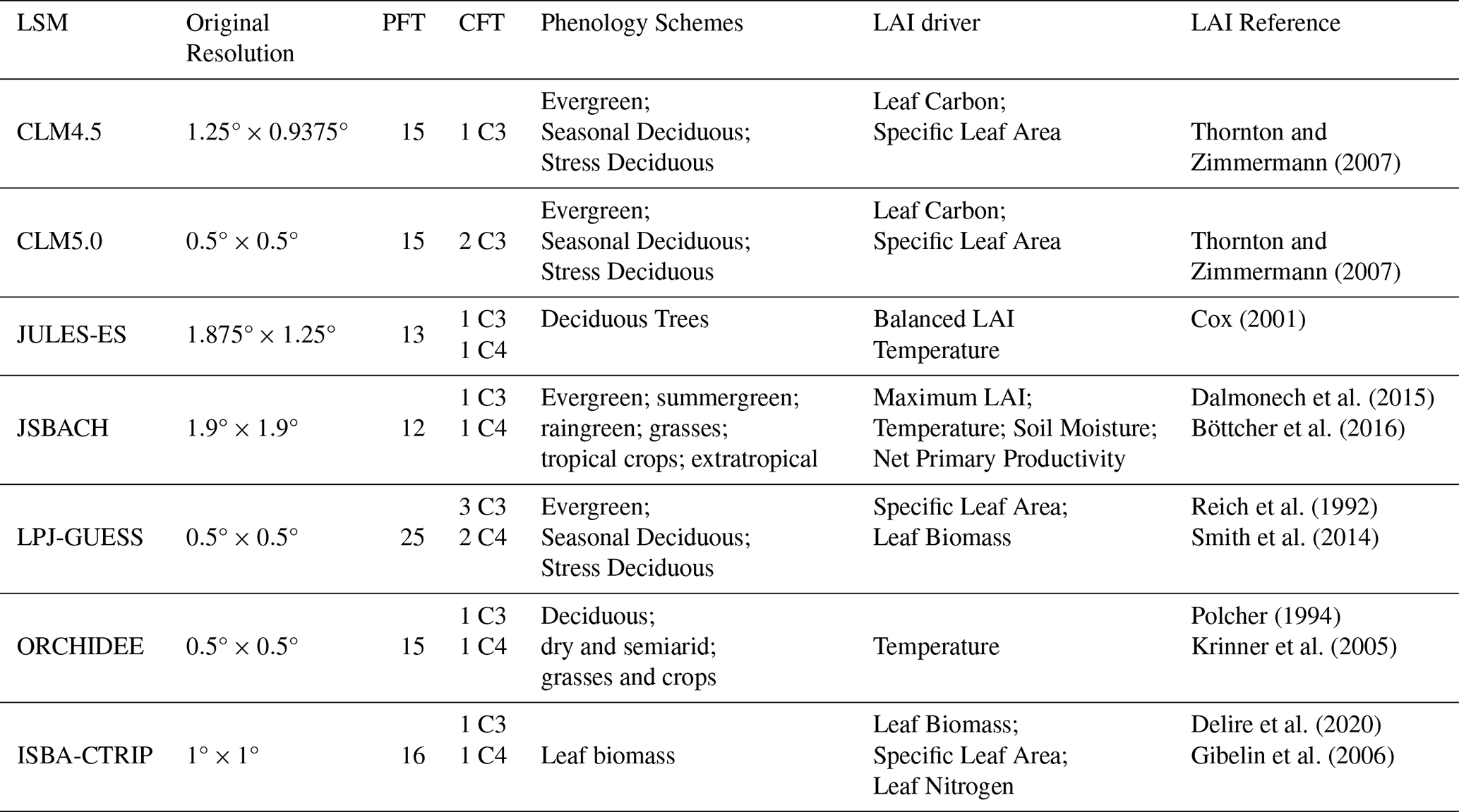
The Community Land Model (CLM) is the terrestrial component of the Community Earth System Model (CESM, http://www.cesm.ucar.edu/, last access: 17 November 2024) and, in its version 4.5 (CLM4.5, Oleson et al., 2013) and biogeochemical configuration (i.e. BGC compset, Koven et al., 2013), it is the land component of the CMCC coupled model version 2 (CMCC-CM2, Cherchi et al., 2019) and Earth System Model version 2 (CMCC-ESM2, Lovato et al., 2022). CLM4.5-BGC features fifteen Plant Functional Types (PFTs), without specific treatment for crop areas. CLM4.5-BGC explicitly resolves carbon-nitrogen biogeochemical cycles (Oleson et al., 2013; Koven et al., 2013), including plant phenology, which is described employing three specific parameterizations: (1) evergreen plant phenology; (2) seasonal-deciduous plant phenology; (3) stress-deciduous plant phenology (Oleson et al., 2013).

CLM version 5.0 (CLM5.0) is the terrestrial component of the Community Earth System Model version 2 (CESM2, http://www.cesm.ucar.edu, last access: 17 November 2024, Danabasoglu et al., 2020) and of the Norwegian Earth System Model (NorESM2, Seland et al., 2020). Compared to the previous version of CLM (i.e. CLM4.5), CLM5 introduces dynamic land units, updated hydrological processes (including revised groundwater scheme, canopy interception and new plant hydraulics functions), revised nitrogen cycling, an improved crop module and various major changes in soil and vegetation parameterization (see Lawrence et al., 2019). Although the phenology scheme of CLM5 is similar to CLM4.5, other model changes (particularly, updated stomatal physiology, nitrogen cycle and plant hydraulics) would indirectly affect the simulated LAI and phenology in CLM5 (see Lawrence et al., 2019; Peano et al., 2021).

JULES-ES is the Earth System configuration of the Joint UK Land Environment Simulator (JULES) and it is the terrestrial component of the UK community Earth System Model (UKESM1, Sellar et al., 2020). JULES-ES implements 13 PFTs in a dynamical vegetation configuration and accounts for a full carbon and nitrogen cycle (Wiltshire et al., 2021). The Leaf Area Index (LAI) varies based on the carbon status and extent of the underlying vegetation (Clark et al., 2011). Phenology operates based on an accumulated thermal time model.

JSBACH3.2 (Reick et al., 2021) is the land component of MPI-ESM1.2 (Mauritsen et al., 2019). JSBACH3.2 implements 12 PFTs, and the LoGro-P model for phenology (Böttcher et al., 2016; Dalmonech et al., 2015). The LoGro-P model uses a logistic equation for the temporal development of the LAI targeting a prescribed PFT-specific physiological limit, independent of the carbon state of the vegetation. JSBACH3.2 distinguishes five phenology types, namely evergreen, summergreen, raingreen, grasses, and tropical and extratropical crops, which is a higher amount of phenology schemes compared to the other land surface models.

LPJ-GUESS is the terrestrial biosphere component of the European Community Earth System Model (EC-Earth-Veg, Döscher et al., 2022). It simulates biogeochemistry cycles, vegetation dynamics, and land use featuring 25 PFTs. Similar to the two CLM models, LPJ-GUESS uses three phenology schemes: (1) evergreen plant phenology; (2) seasonal-deciduous plant phenology; (3) stress-deciduous plant phenology.

ORCHIDEE is the land component of the IPSL (Institut Pierre Simone Laplace) Earth System Model used in the CMIP6 effort (Boucher et al., 2020). ORCHIDEE features 15 PFTs that vary based on the LUH2 forcing (Lurton et al., 2019). The phenology module describes leaf onset and senescence based on temperature and soil moisture (Botta et al., 2000).

ISBA-CTRIP is the land component of CNRM-ESM2-1 (Séférian et al., 2019) and it works within the SURFEX version 8 modelling platform. It accounts for 16 vegetation types alongside desert, rocks and permanent snow (Decharme et al., 2019). Differently from the other land surface models, ISBA-CTRIP computes the leaf phenology based on the daily carbon balance of the leaves as described in Delire et al. (2020).

2.3 Experimental setup

All LSMs were forced by near-surface atmospheric variables (2 m air temperature, precipitation, wind, surface pressure, shortwave radiation, longwave radiation, and air humidity) from the CRUNCEP version 7 reanalysis dataset (Viovy, 2018), following the TRENDY protocol (Sitch et al., 2015; Zhao et al., 2016), and land cover values from the Land Use Harmonization version 2 (LUH2, Hurtt et al., 2020). Despite each LSM implementing the LUH2 data differently (e.g. different number of PFTs), the same vegetated areas evolution forces them to leave differences in plant growth, biodiversity, and seasonality among them.

LSM simulations cover 1850–2014, following the historical period, as defined in CMIP6 (Eyring et al., 2016). Consequently, the comparison between models and satellite data covers the shared period from 2000 (the starting year of MODIS data) to 2011 (the last available year of LAI3g), as done in the companion paper (Peano et al., 2021).

To facilitate intercomparison across models and satellite data, modelled LAI on Plant Functional Types (PFT) were weighted averaged by PFT fraction for each grid box to produce an estimate of grid box mean LAI for all models. As each LSM was run on a different grid resolution (Table 1), to enable cross-analyses the model outputs and satellite data used in this study were expressed as monthly means and regridded to a regular 0.5°×0.5° grid using the Climate Data Operators (CDO) toolset first order conservative remapping scheme (Jones, 1999; Schulzweida, 2019).

2.4 Growing season analyses

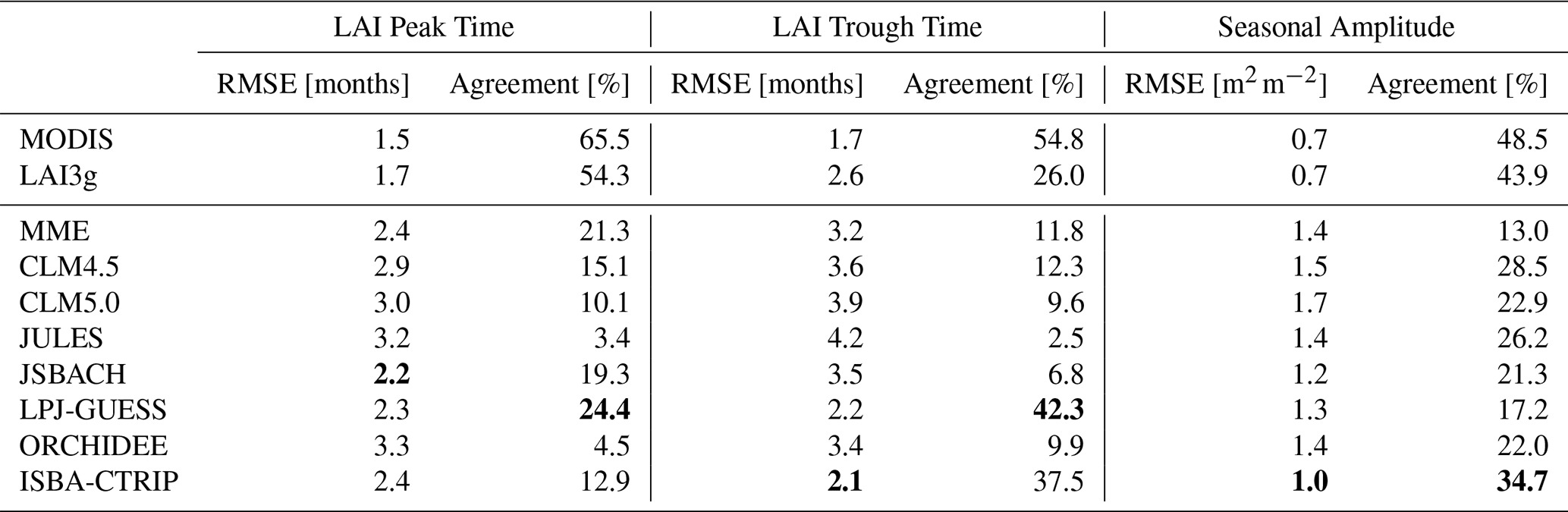
Global variations in the monthly mean quantity, timing, and amplitude of annual LAI peaks and troughs (2000–2011 mean) derived from the satellite products (Sect. 2.1) are compared with the LSM estimates (Sect. 2.2) of the same variables. Peaks are identified as the month with the highest LAI value, representing the apex of the vegetation life cycle. On the contrary, the troughs are identified as the months with the lowest LAI value, depicting the plant's dormancy season. For a situation where the same minimum or maximum LAI values are recorded in multiple months per year, the first month in the year with that value is retained as the peak or trough. The values of peak and trough are computed for each of the satellite observation datasets and land surface models. Results from the land surface models are also aggregated and evaluated as a multi-model ensemble mean (MME). Finally, the agreement between LSMs and satellite products refers to differences of 0 months in peak and trough (i.e. both LSM and satellite product produce peak and trough occurring in the same month) and of 0.25 m² m⁻² in LAI amplitude.

3 Results

3.1 Growing season peak and trough

3.1.1 Satellite estimates

The annual timing of peak LAI (monthly mean) estimated from the three satellite products is broadly consistent (±1 month) across global biomes (∼60 % of the globe, Fig. 1, and Table 2). However, in specific locations, these satellite estimates differ in the month of peak LAI by up to 3 months – notably in central/western Australia, tropical Africa and South America and in patches across other biomes globally, with the LAI3g estimates showing the latest annual peaks (leading to root mean square differences of 1.5–1.7 months, Table 2). The timings of LAI trough are less consistent between satellite products (agreement between 26 % and 54 %, Table 2). Across many regions of the globe, the LAI3g trough estimates are 1 to 3 months later than the CGLS and MODIS estimates, although in the western Amazon basin and in patches across the northern boreal zone LAI3g trough estimates are earlier (up to 3 months) than CGLS or MODIS (LAI3g root mean square error of 2.6 months, Table 2). The differences in boreal regions derive from discrepancies in the gap-filling approaches applied to high-latitude winter values between satellite products, which is a relevant limitation of satellite products, as discussed in Sect. 4.4. The longest differences in the timing of troughs between satellite products are in central/western Australia, southern Africa, tropics, central and east Asia, eastern North America, and across the boreal zone. These discrepancies between satellite products exhibit the range of observational uncertainties, which derive from differences in LAI reconstruction approaches, sensors, and orbits, as further discussed in Sect. 4.4.

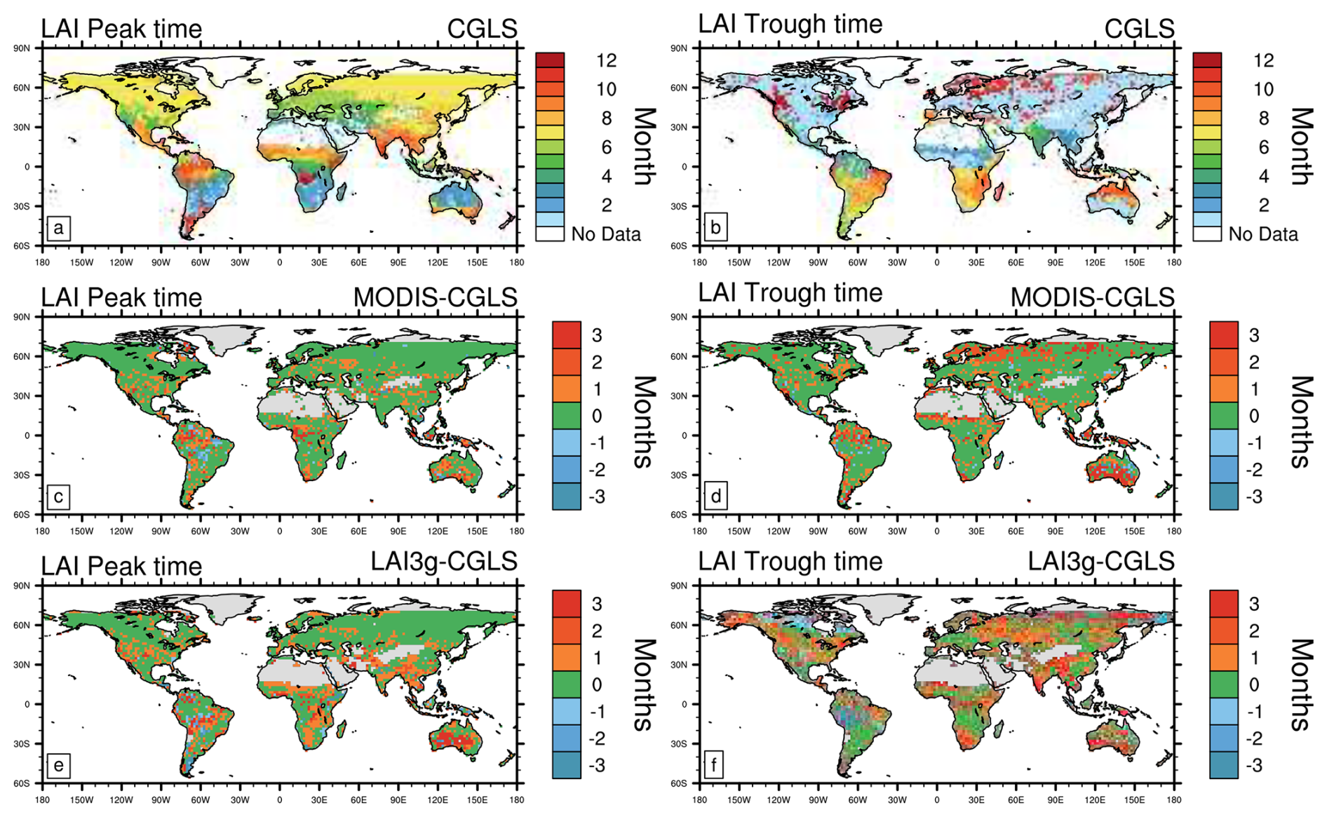
Figure 1 Comparison of satellite data estimates of the month of Leaf Area Index (LAI) peak (left) and trough (right) for: (a, b) CGLS, and differences (in months) between (c, d) MODIS and CGLS, and (e, f) LAI3g and CGLS. Note that positive values stand for delayed peak or trough timings compared to CGLS ones. Additionally, LAI data are available from 56° S to 72° N, which is the range covered by CGLS.

Table 2 Root mean square error (in month and m² m⁻²) between CGLS and the other satellite products (first two rows of the table) and land surface models (last eight rows of the table) and the percentage of the region in agreement (green areas in Figs. 1, 2, 3, 5, and 6) with the CGLS values. Note that the best score values among LSMs are bold.

3.1.2 Modelled estimates

Compared with the CGLS satellite estimates, most LSMs show widespread delay (up to 3 months, MME root mean square error of 2.4 months, Table 2) in the estimated LAI peak (Fig. 2). This is most notable across northern hemisphere temperate and boreal zones, in parts of central and southern Africa, and central South America, as indicated by the multi-model ensemble mean (MME). On the contrary, LSMs exhibit earlier LAI peaks in southern South America and the Amazon and Congo basins. Finally, some LSMs show agreement with CGLS in the timing of LAI peak in the central US and Indian peninsula. In general, LPJ-GUESS shows the most widespread agreement in the timing of the LAI peak with the satellite products (24.4 % of the land area, Fig. 2f and Table 2), despite JSBACH exhibits a smaller bias compared to the other LSMs (root mean square error of 2.2, Table 2).

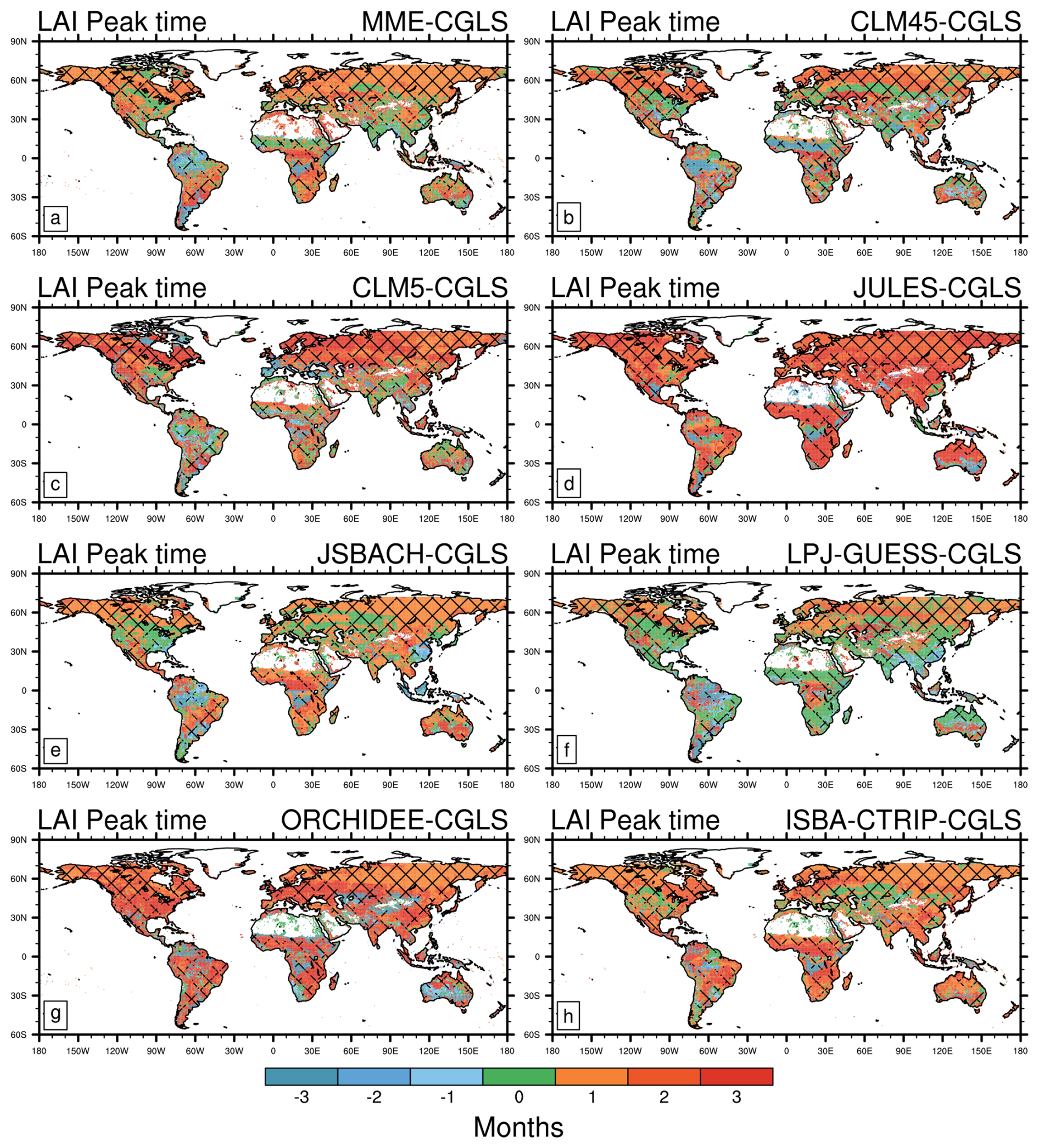
Figure 2 Difference in monthly mean Leaf Area Index (LAI) peak timing between CGLS satellite observations and modelled estimates from: (a) Multi Model Mean (MME); (b) CLM4.5; (c) CLM5.0; (d) JULES; (e) JSBACH; (f) LPJ-GUESS; (g) ORCHIDEE; (h) ISBA-CTRIP. Areas of agreement between satellite products are shaded with different hatching patterns: CGLS and LAI3g (Fig. 1e) slash hatching ($/$); CGLS and MODIS (Fig. 1c) backslash hatching (\); CGLS, MODIS, and LAI3g crossed hatching (X). Note that positive values stand for delayed peak timings compared to CGLS ones. Additionally, LAI data are available from 56° S to 72° N, which is the range covered by CGLS.

Similar differences between LSMs and satellites are visible in the LAI trough (Fig. 3). The majority of LSMs show widespread delays (up to 3 months, MME root mean square error of 3.2 months, Table 2) in the LAI trough, except in some areas of South America, South Africa, and India where LSM and satellite estimates are in reasonable agreement, as indicated by the multi-model ensemble (MME). On the contrary, earlier LAI trough timings (up to 2 months) are displayed for some LSMs in Northern Australia, southern Africa, tropical South America, and some areas above 60° N (Fig. 3a). Similar to the LAI peak, LPJ-GUESS shows the most widespread agreement in the timing of the LAI trough with the satellite products (42.3 % of land area, Fig. 3f and Table 2). ISBA-CTRIP, instead, exhibits valuable results in the northern hemisphere (agreement in 37.5 % of land area, Fig. 3h and Table 2).

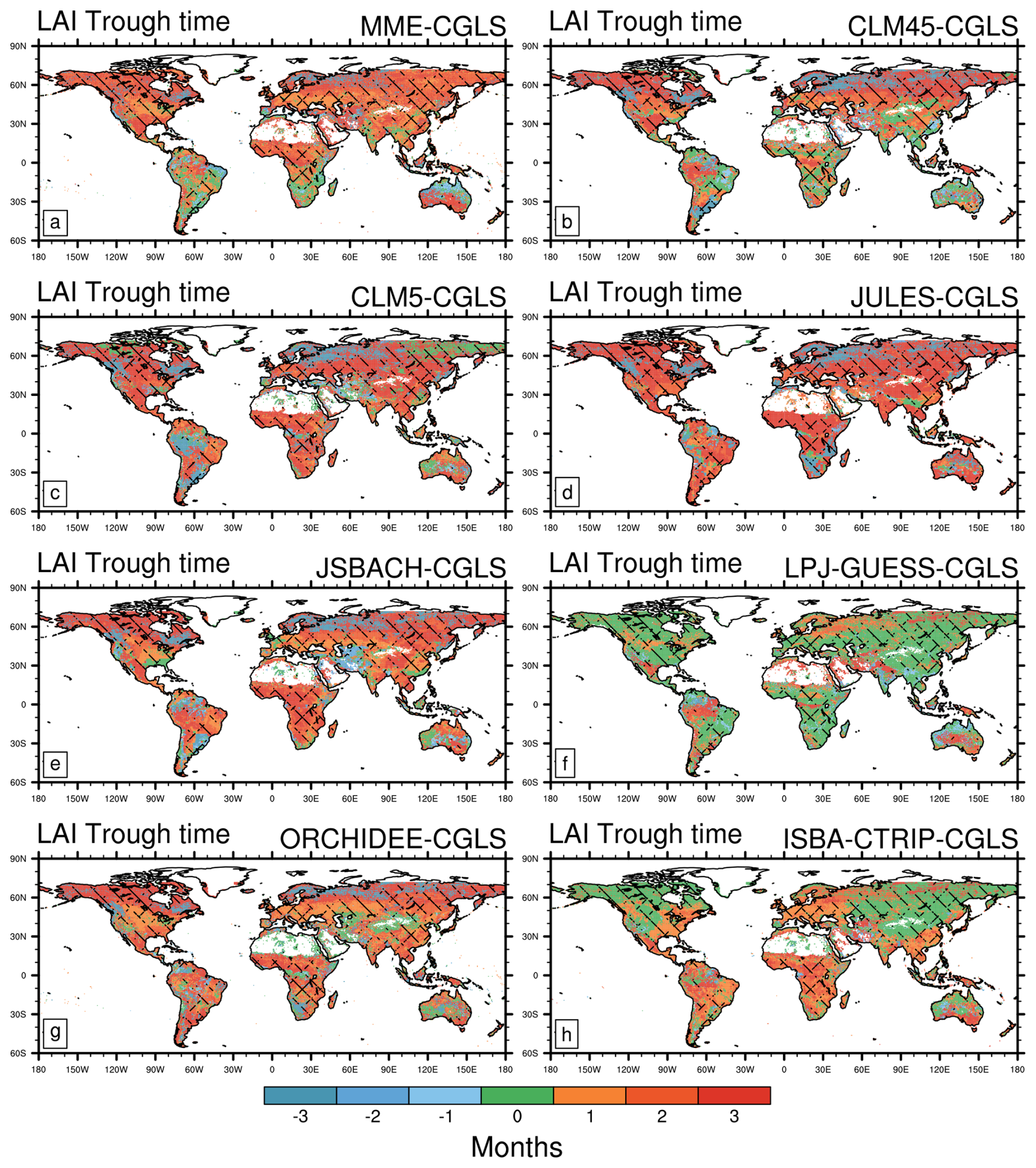
Figure 3 As in Fig. 2 but for Leaf Area Index (LAI) trough. Areas of agreement between satellite products are shaded with different hatching patterns: CGLS and LAI3g (Fig. 1f) slash hatching ($/$); CGLS and MODIS (Fig. 1d) backslash hatching (\); CGLS, MODIS, and LAI3g crossed hatching (X). Note that positive values stand for delayed trough timings compared to CGLS ones. Additionally, LAI data are available from 56° S to 72° N, which is the range covered by CGLS.

Based on these results, the high vegetation heterogeneity represented by LPJ-GUESS (due to both the number of PFTs and CFTs, and original resolution, Table 1) provides a better agreement with CGLS compared to the other LSMs, especially in trough timings, where also ISBA-CTRIP (the second LSM in number of PFTs, Table 1) shows high agreement with CGLS. On the contrary, the variety of phenology schemes may improve the ability to capture the correct timings, as done by JSBACH, which distinguishes up to six phenology schemes (Table 1), in peak timings (Fig. 2).

3.1.3 Latitudinal variability

The timing of LAI peaks and troughs simulated by the LSMs show good agreement with the satellite products across tropical areas, between 30° N and 30° S, and differences of several months outside of this zone (Fig. 4a). Across the northern hemisphere temperate and boreal zones, north of 30° N, LSM show consistently later LAI peaks driven by a delayed start of the growing season (Fig. 4 in Peano et al., 2021). Below 30° S, satellite products and LSMs display a large variability. The large difference at those latitudes between LAI3g and MODIS and CGLS mainly resides in the reconstruction of LAI values in southern hemisphere semiarid regions (Fig. 1e). On the contrary, the LSMs display widespread differences with CGLS in the southern hemisphere (Fig. 2), highlighting a much higher coherence among LSMs' LAI parameterization in boreal and temperate regions.

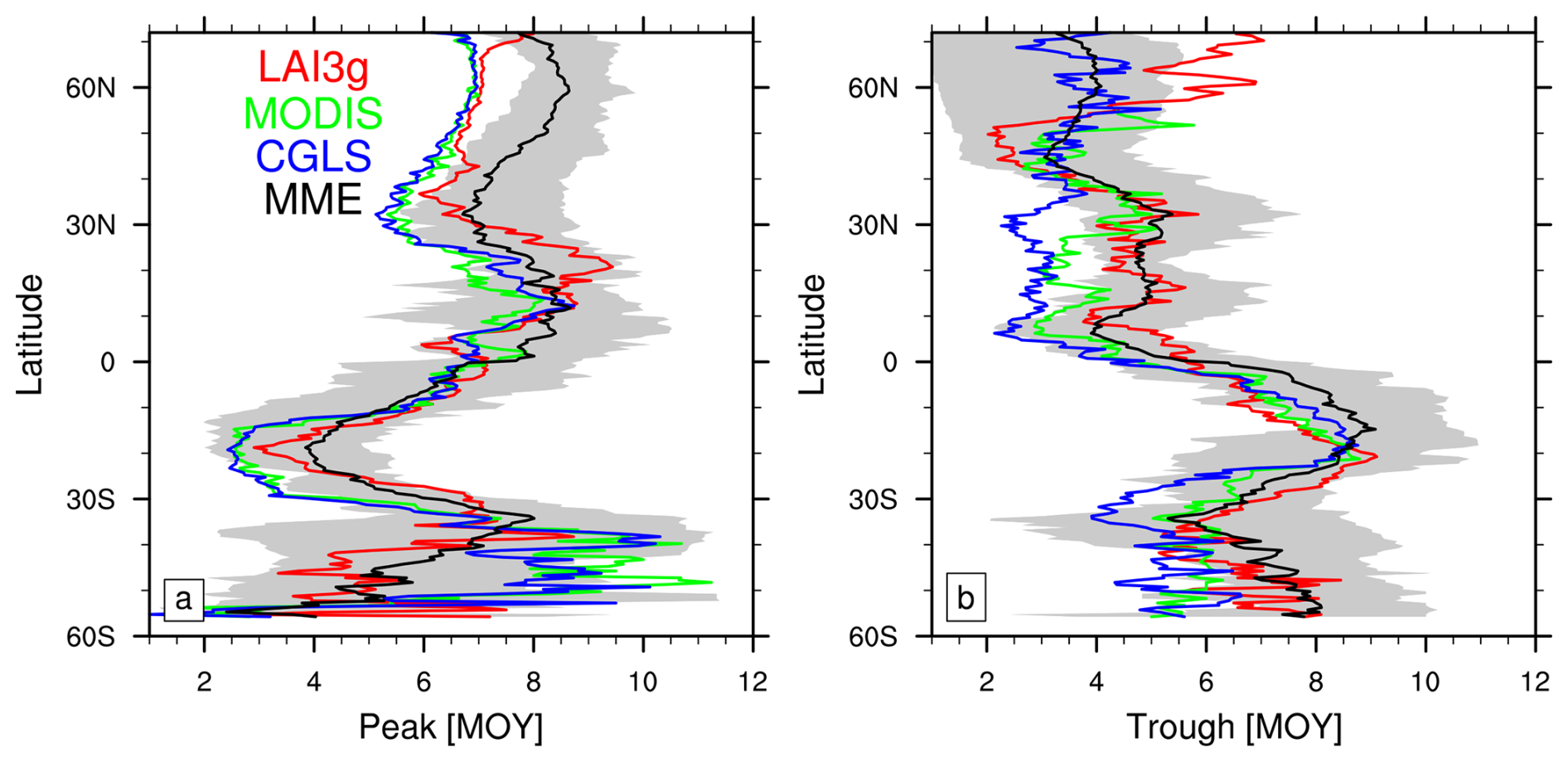
Figure 4 Zonal monthly mean timing of Leaf Area Index (LAI) (a) peak and (b) trough for LAI3g (red lines), MODIS (green lines), CGLS (blue lines), and multi-model ensemble mean (MME, black line). The grey regions show the multi-model ensemble spread. Values are reported as month of the year (MOY), and the latitudinal coverage is from 56° S to 72° N, which is the range covered by CGLS.

Differently from peak timings, the MME latitudinal distribution of trough timings exhibits minor differences with satellite products (Fig. 4b) thanks to a higher variability among satellite records. The LSMs show delayed trough timings (centred around June) in the northern hemisphere tropical region (0–30° N) compared to the MODIS and CGLS datasets (between February and May) but reasonable agreement with LAI3g.

In the trough case, a larger variability among LSM and satellite products occurs above 55° N, which derives from the approach used in reconstructing winter LAI values. In particular, MODIS displays no values in trough timing above 55° N. This behaviour derives from the absence of LAI data in those regions during the polar nights, which correspond to the season during which trough timings occur.

3.2 LAI seasonal amplitude

3.2.1 Satellite estimates

There is widespread consistency in the LAI seasonal amplitude (LAI maximum minus LAI minimum) estimated from the three satellite products (root mean square error of 0.7 m² m⁻², Table 2), with spatial differences usually less than 1 m² m⁻² (Fig. 5) and agreement in the range from −0.25 to 0.25 m² m⁻² in about 45 % of the land regions (Table 2). However, these differences are larger across areas of the boreal and tropical forests where both LAI3g and MODIS show a higher (up to 2.5 m² m⁻²) seasonal amplitude than CGLS. The discrepancies in tropics are mainly driven by mismatches in minimum LAI values between the three satellite datasets (Fig. S1 in the Supplement). On the contrary, dissimilarities in maximum LAI values drive the differences in boreal regions (Fig. S2).

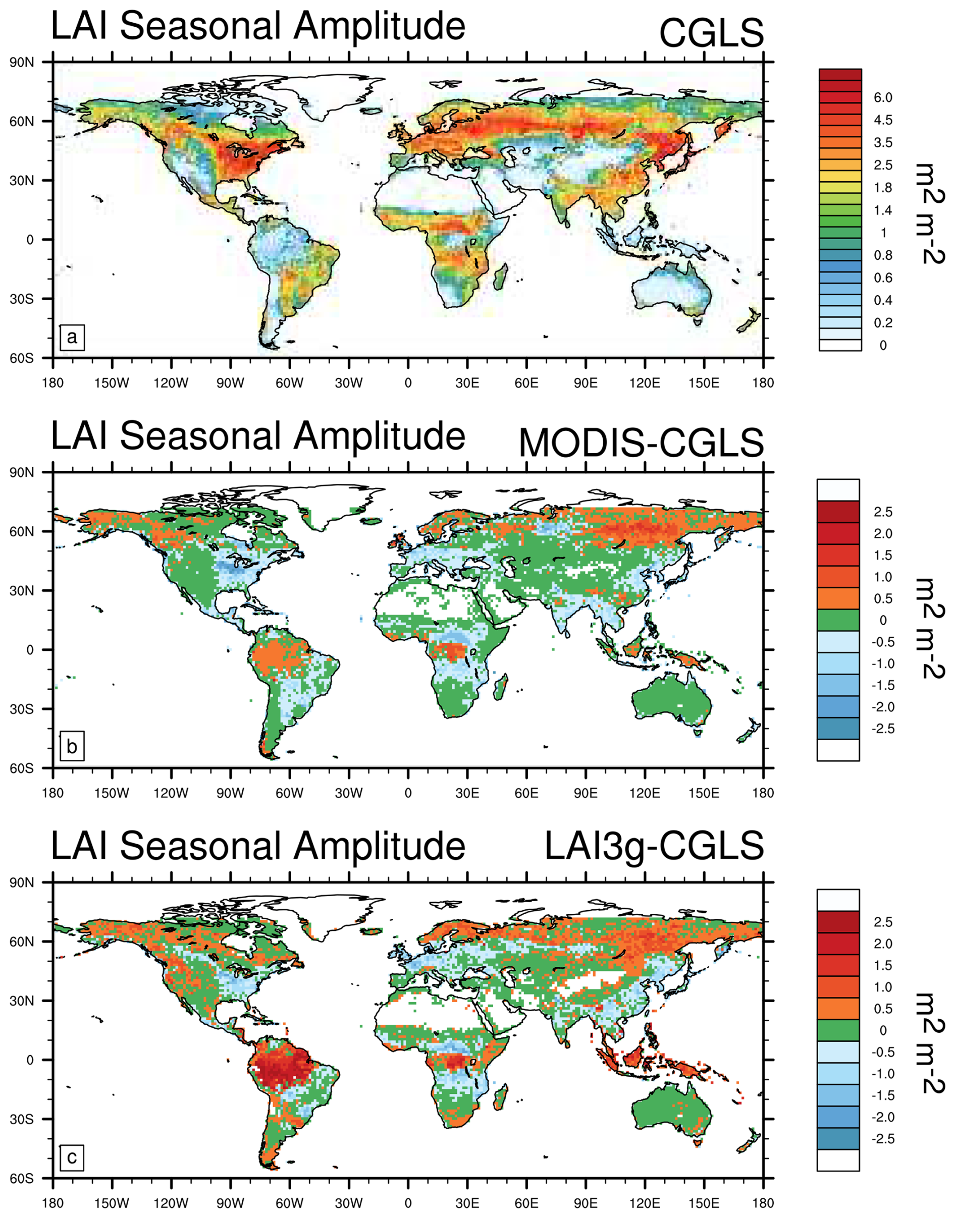
Figure 5 Comparison of satellite data estimates of the Leaf Area Index (LAI, in m² m⁻²) seasonal amplitude (maximum LAI minus minimum LAI) reported in m² m⁻² for (a) CGLS, and differences between CGLS and (b) MODIS, and (c) LAI3g. Note that LAI data are available from 56° S to 72° N, which is the range covered by CGLS.

3.2.2 Modelled estimates

Compared with the CGLS satellite estimates of seasonal amplitude (Fig. 5), LSMs show broadly consistent values with root mean square differences ranging between 1.0 (ISBA-CTRIP) and 1.7 (CLM5.0) m² m⁻² (Table 2). The majority of LSM exhibit agreement with satellites in the Amazon, Australia, and western North America (Fig. 6) with an agreement in MME in about 13.0 % of the land areas (Table 2).

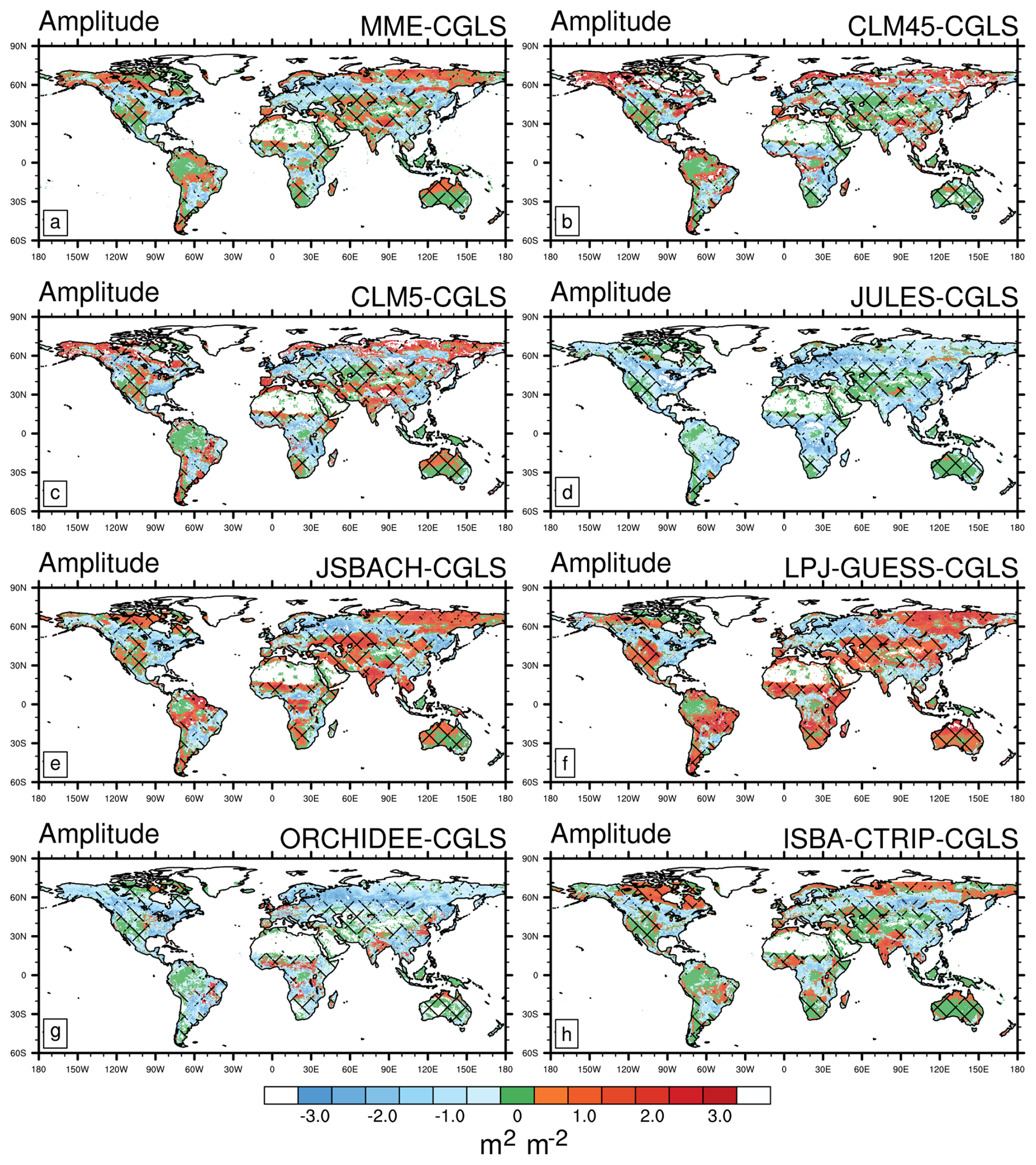
Figure 6 As in Fig. 2 but for Leaf Area Index (LAI) seasonal amplitude (maximum LAI minus minimum LAI) reported in m² m⁻². Areas of agreement between satellite products are shaded with different hatching patterns: CGLS and LAI3g (Fig. 5c) slash hatching ($/$); CGLS and MODIS (Fig. 5b) backslash hatching (\); CGLS, MODIS, and LAI3g crossed hatching (X). Note that LAI data are available from 56° S to 72° N, which is the range covered by CGLS.

In general, LSMs simulate a smaller LAI seasonal amplitude compared to CGLS, especially in boreal forests and areas of Africa and South America (Fig. 6a). JULES and ORCHIDEE exhibit smaller LAI seasonal amplitude compared to CGLS and other LSMs in broader areas (Fig. 6d and g). However, this result is achieved by a bias compensation in maximum and minimum LAI values by JULES (Figs. S3d and S4d), while ORCHIDEE agrees with CGLS also in both components (Figs. S3g and S4g). On the other hand, LPJ-GUESS displays widespread areas of wider LAI seasonal amplitude compared to satellites and the other LSMs in Asia, Africa, and South America (Fig. 6f). This behaviour arises from overestimation in maximum LAI values (Fig. S4f).

Among the LSMs, ISBA-CTRIP exhibits the best agreement and the lowest error compared to CGLS in seasonal LAI amplitude. This behaviour mainly derives from the ability of ISBA-CTRIP to capture the minimum LAI values (Fig. S3h), combined with low biases in maximum LAI (Fig. S4h). This ability could originate from a better inclusion of the nitrogen cycle within the LAI computation (Table 1).

3.2.3 Latitudinal variability

The LAI seasonal amplitude simulated by LSMs shows reasonable agreement with satellite products in the southern hemisphere and between 20 and 40° N (Fig. 7). LSMs exhibit smaller differences between maximum and minimum LAI in the areas above 40° N compared to the observations. Finally, the satellite products show disagreement in the areas around the equator (i.e. 10° S–10° N), where LAI3g shows larger seasonal amplitude compared to CGLS, MODIS and LSMs. MODIS tends to have LAI seasonal amplitude values slightly smaller than LAI3g and CGLS, with a prominent difference in the region between 30 and 45° S.

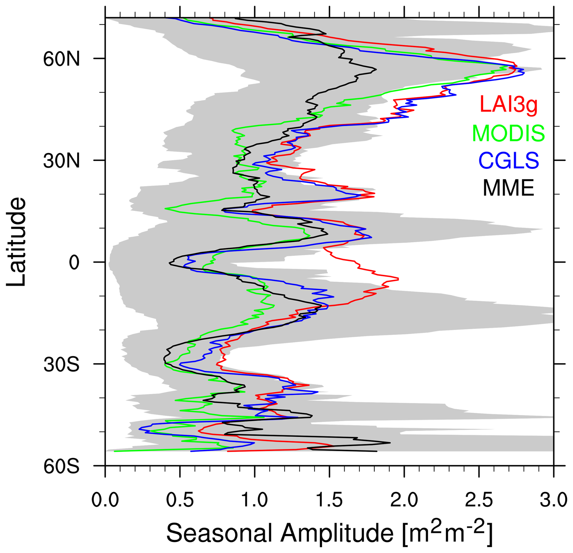
Figure 7 Zonal monthly mean Leaf Area Index (LAI) seasonal amplitude (maximum LAI minus minimum LAI) for LAI3g (red lines), MODIS (green lines), CGLS (blue lines), and multi-model ensemble mean (MME, black line). The grey regions show the multi-model ensemble spread. Values are reported in m² m⁻² and the latitudinal coverage is from 56° S to 72° N, which is the range covered by CGLS.

In general, LSMs exhibit a large variability among them that peaks around 20° S and 10° N, which are transitional areas, and below 50° S and above 60° N where LSMs may differ in the representation of these areas characterised by Arctic vegetation.

3.3 Regional variability

At the biome scale, the LAI peak timings estimated by the LSMs are generally delayed compared to the satellite estimates, particularly across regions dominated by both needleleaf and broadleaf trees (Fig. 8b–e, i, and j). An exception is for broadleaf evergreen trees (BET) in both hemispheres (Fig. 8d and i). In the regions dominated by BET (about 11 % of the vegetated regions), the simulated LAI peak values fall in the 25$/$75 percentile distribution of the satellite estimates (Fig. S5). The peak of broadleaf deciduous shrubs (BDS) in the northern hemisphere is also delayed compared to CGLS, MODIS, and LAI3g (Fig. 8f), which is not the case in the southern hemisphere for the MME (Fig. 8k). However, the LSMs exhibit large variability in the BDS biome (Fig. S5k). Similar hemispheric behaviour is observed in grass-dominated areas (Fig. 8g and l), while the crop biome is reasonably well captured (Fig. 8h and m).

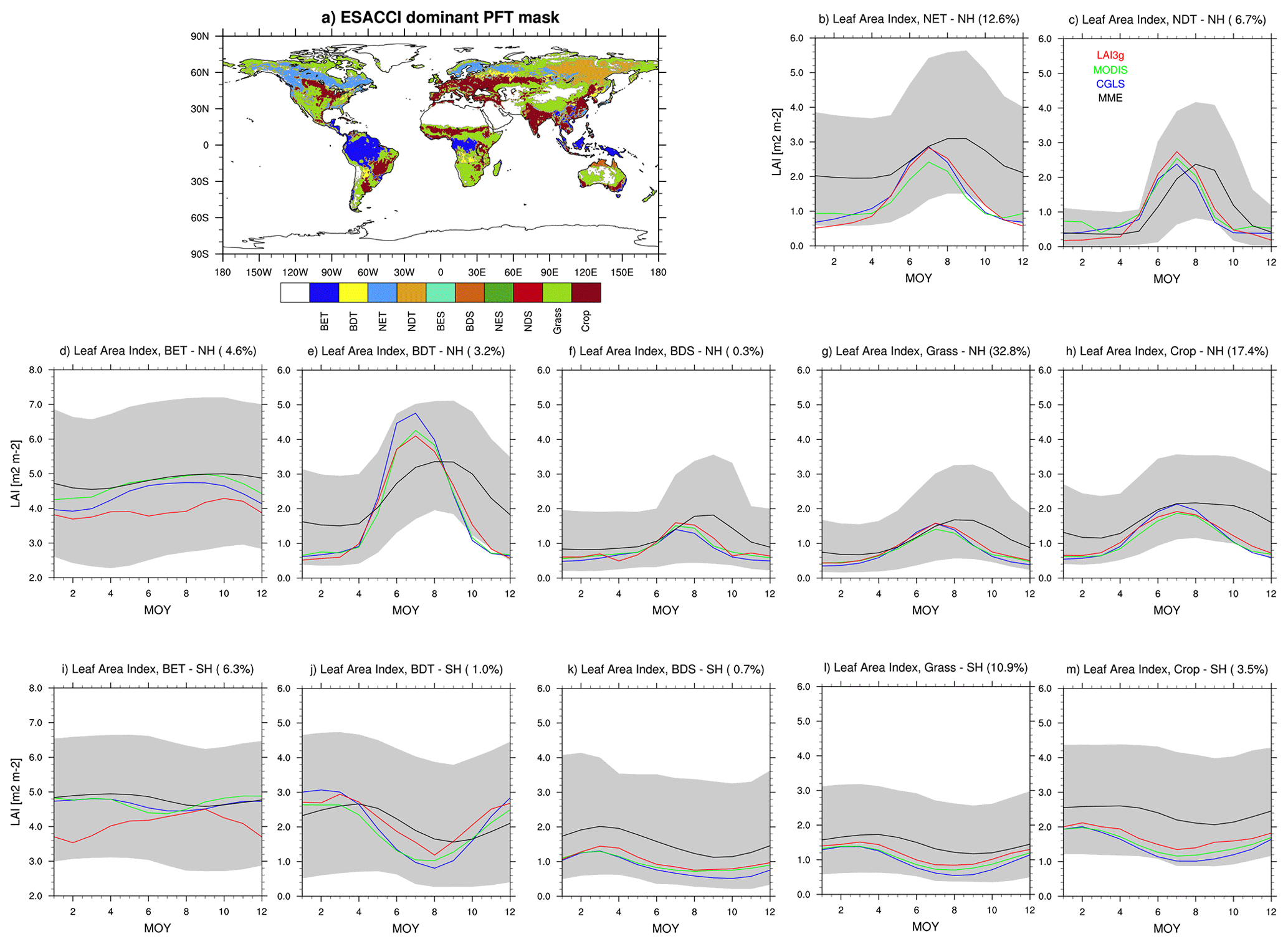
Figure 8 (a) Global distribution of the main land cover types for the 2000–2011 period based on ESA CCI data (Li et al., 2018). Comparison in the Leaf Area Index (LAI) timeseries between satellite products (CGLS, red; MODIS, green; LAI3g, blue) and land surface models (LSMs: CLM4.5, CLM5.0, JSBACH, JULES, LPJ-GUESS, ORCHIDEE, ISBA-CTRIP) Multi Model Mean (black) and model spread (grey shadow) in (b) needle-leaf evergreen tree (NET) in the Northern Hemisphere (NH); (c) needle-leaf deciduous tree (NDT) in the NH; broadleaf evergreen tree (BET) in the (d) NH and (i) SH; broadleaf deciduous tree (BDT) in the (e) NH and (j) SH; broadleaf deciduous shrub (BDS) in the (f) NH and (k) SH; grass-covered areas (Grass) in the (g) NH and (l) SH; and crop-covered areas (Crop) in the (h) NH and SH (m). Note that no area is dominated by broadleaf evergreen shrub (BES), needle-leaf evergreen shrub (NES), or needle-leaf deciduous shrub (NDS) biome. Note that the y axis is different in the BET panels, but all y axis cover a 6 m² m⁻² LAI range. Additionally, the percentage of global vegetated area covered by each biome is displayed in the title of each panel.

The LAI trough timings estimated by the LSM are generally delayed compared to the satellite estimates in regions dominated by needleleaf trees (NDT, NET), broadleaf deciduous trees (BDT), Crop, and northern hemisphere Grass (Fig. 8b, c, e, g, h, j, and m). The trough timings of Broadleaf Evergreen Trees (BET, Fig. 8d and i), especially in the northern hemisphere (Fig. 8d), and Broadleaf Deciduous Shrubs (BDS, Fig. 8f and k), and southern hemisphere Grass (Fig. 8l) show values in agreement with satellite values (see also Fig. S6).

In general, the growing seasons simulated by the LSM show delays in their peaks compared to the satellite estimates, especially in the northern hemisphere. Moreover, LSMs sharing similar phenology parameterisation schemes, such as CLM4.5, CLM5.0, and LPJ-GUESS (Table 1), display discrepancies in phenophases estimates, such as in the southern hemisphere BET biome, where CLM5.0 differs from CLM4.5 and LPJ-GUESS by approximately 6 months (Figs. S5i and S6i). This behaviour highlights the influence of models' features beyond the specific phenology schemes in representing the growing season cycle.

Focusing on seasonal amplitude, LSMs tend to simulate smaller seasonal amplitude in the areas dominated by needleleaf trees (Fig. 8b and c). This behaviour is mainly driven by ORCHIDEE (Fig. S7b and c). Reduced differences between LAI maximum and minimum are also simulated in the Broadleaf Deciduous Tree (BDT) biome (Fig. 8e and j), mainly due to JULES-ES (Fig. S7e and j). The seasonal amplitude is reasonably well captured in the Grass- and Crop-dominated areas (Fig. 8g, h, l, and m). The Broadleaf Deciduous Shrub (BDS) biome exhibits seasonal amplitude in line (Northern Hemisphere, Fig. 8f) or slightly longer (Southern Hemisphere, Fig. 8k) compared to satellite products. Finally, the regions dominated by Broadleaf Evergreen Trees (BET) display simulated seasonal amplitude values in agreement with CGLS and MODIS but smaller than LAI3g (Figs. 8d, i and S7d, i).

Several LSMs represent LAI values based on the values of specific leaf area and the amount of leaf carbon or biomass content (i.e. CLM4.5, CLM5.0, LPJ-GUESS, and ISBA-CTRIP, Table 1). The implementation of similar parameterisation reflects on reduced differences between LSMs (Fig. S7), except for southern hemisphere BDS-dominated areas (Fig. S7k), where LPJ-GUESS substantially overestimates the LAI seasonal amplitude compared to CLM4.5, CLM5.0 and ISBA-CTRIP. On the other hand, LSMs primarily driven by temperature, such as JULES-ES and ORCHIDEE, tend to underestimate the LAI seasonal amplitude (Fig. S7), which is not the case when also leaf features are considered, as done in JSBACH (Table 1). This comparison, then, underscores the need to incorporate leaf features and leaf carbon content in LAI computation within LSMs.

4 Discussion

4.1 LAI peak and trough versus seasonal amplitude

The LAI simulated by LSM shows differences with satellite products in both the timings (i.e. peak and trough) and the quantities (i.e. seasonal amplitude). Since these two metrics (i.e. timings and quantities) assess different vegetation features, there is no clear consistency between them. For example, JULES shows a general underestimation of seasonal amplitude compared to CGLS (Fig. 6d) with peak and trough timings dominated by delayed values (Figs. 2d and 3d). Similar delayed peak and trough timings are simulated by CLM5, ORCHIDEE and partially JSBACH (Figs. 2c, e, g and 3c, e, g) yet for these models an underestimation in seasonal amplitude is only noted for ORCHIDEE (Fig. 6g), CLM5 and JSBACH show a mixture of positive and negative differences in seasonal amplitude (Fig. 6c and e). On the other hand, LPJ-GUESS shows peak and trough timings that are reasonably close to the satellite estimates (Figs. 2f and 3f), while the seasonal amplitude for this model is broadly overestimated (Fig. 6f).

This behaviour emphasises the detachment between LSM ability in representing the vegetation timings (i.e.phenology) and quantity, as previously presented for CLM4.5 in Peano et al. (2019) even if the same variable, i.e. LAI, can be applied in assessing both metrics. These differences derive from the different forcings for vegetation timings, usually determined by temperature, soil moisture, solar radiation, and quantity, which is co-determined by climate forcing, photosynthesis and carbon and nitrogen allocations. Consequently, both metrics need to be considered when evaluating LSMs, as done here.

4.2 Comparison with onset and offset evaluation in Peano et al. (2021)

LSMs show a delayed peak in forested areas compared to satellite estimates combined with a delayed start of the growing season, as shown in Fig. 7 by Peano et al. (2021), suggesting a possible modelled too-slow leaf production. LSMs also exhibit a delay in trough timings (Chen et al., 2020; Jeong, 2020), suggesting a general shift in the growing season (Fig. 8 and proposed in the companion paper Peano et al., 2021). The assessment of the start, peak, and end of the growing season timings points out a temporal shift of the vegetative active season in LSMs compared to satellite records. Nevertheless, only in limited areas (between 17 % and 35 % of vegetated areas, Table 3 in Peano et al., 2021) LSMs correctly reproduced growing season length.

The combination of the results from the present study and its companion (Peano et al., 2021) highlights LSMs' limitations in correctly capturing timings, amplitude, and length of the vegetative active season pointing at the need for further development of vegetation phenology, distribution, and mass representation in the LSMs. In general, LSMs should improve their ability to capture vegetation heterogeneity in both plant traits, such as a higher number of PFTs, and phenology features, for example, by increasing the variety of phenology schemes to enhance their ability to represent vegetation responses to various stresses.

4.3 Sources of variability between land surface models

The LSMs involved in this study and its companion (Peano et al., 2021) use state-of-the-art boundary conditions (i.e. atmospheric and land use forcings). The LUH2 land-use evolution (Hurtt et al., 2020) employed in the CMIP6 effort is used in this study. It is noteworthy that each LSM implements the same land-use boundary conditions differently due to dissimilarities in the original resolution, number of PFTs, and land-use scheme implemented in each model (Table 1). Nonetheless, the implementation of a common land-use dataset allows all LSM to reproduce the same vegetated areas evolution, leaving only differences in plant growth, biodiversity, and seasonality among them. Besides, the same set of atmospheric variables has been used to force all the LSMs following the TRENDY protocol (Sitch et al., 2015; Zhao et al., 2016). However, the atmospheric conditions (e.g. temperature and water availability) strongly influence the vegetation growth, and a different source of atmospheric forcing may partially affect the biases obtained in this study. For example, the ISBA-CTRIP model forced by WFDEI forcing (Weedon et al., 2014) exhibits smaller biases compared to the present results (Dewaele et al., 2017).

Despite using the same boundary conditions (atmospheric and land use forcings), the variability between the LSM may derive from various sources, such as differences in vegetation parameterization, crop and plant functional type population, soil characterization, and initial spatial resolution, as already noted in Peano et al. (2021). In particular, the discrepancies in model grid resolution and a relatively coarse initial spatial resolution (between about 2° and 0.5°, Table 1) induce differences in the simulated grid vegetation mixture, which may explain the mismatch between LSMs, especially in regions characterised by high biodiversity and areas with evergreen forests. The availability of data at the PFT level would reduce the resolution impact and refine the investigation of differences between LSMs as requested for the next phase of the Coupled Model Intercomparison Project (CMIP7, Li et al., 2025). In general, the results of this study highlight the relevance for LSMs to capture the high vegetation heterogeneity on both PFTs and CFTs populations, that is the case for LPJ-GUESS, and phenology schemes, as for JSBACH.

Moreover, vegetation parameterizations used in the LSM are based on data from localised areas, typically located in the northern hemisphere (e.g. Thornton and Zimmermann, 2007), which may lead to a possible misrepresentation of south hemisphere features. Consequently, the parameters used in LSMs need to be calibrated against more recent and widespread observations.

The results presented in this study highlight a prevalent delay in plant active season compared to observations, despite each LSM implementing different parametrization and processes, emphasising the need for further investigation of the representation of the processes involved in the start of the growing season within the LSMs.

In addition, the case of the Community Land Model provides an example of the impact of model structure versus parameterization on simulated LAI. In the present study, CLM is evaluated in two versions, namely CLM4.5 and CLM5.0. The latter contains various changes in the representation of soil, plant hydrology and carbon and nitrogen cycles (i.e. model structure, Lawrence et al., 2019), influencing the simulated vegetation quantity (see differences in seasonal amplitude in Fig. 6). On the other hand, CLM5.0 applies limited modifications to the phenology parameterization, resulting in minimal differences in the biases of growing season timings compared to its earlier version (Figs. 2b and c and 3b and c), as also shown in Li et al. (2022b). The comparison between CLM versions, then, stresses the separate influence of model structure and phenology parameterization on the simulated LAI features. Moreover, both CLM4.5 and CLM5.0 implement the same LUH2-derived PFT distribution, avoiding the influence of mismatched vegetation type in this version comparison. In general, it highlights the complexity of modelling land surface and vegetation processes and the need for further model development and evaluation.

Finally, a detailed comparison between phenology parameterizations requires data at the PFT level and a mapping between PFTs and phenology schemes as done by Li et al. (2024a) and requested in the next Coupled Model Intercomparison Project phase (CMIP7, Li et al., 2025). The availability of that information will provide the possibility to improve our knowledge of the limitations and abilities of each phenology scheme.

4.4 Satellite products caveats and differences

Despite the satellite datasets agreeing in about half of the vegetated regions (Table 2), differences emerge between them (Table 2), even with peaks of up to 3 months in timings and above 1 m² m⁻² in magnitude in limited areas, but smaller than the differences between LSMs and satellite records. The discrepancies between the three products may be caused by differences in their satellite types and orbits, spectral sensors, LAI estimation approaches, and other technical differences (monthly averaging, gap filling, reflectance saturation, and spatial interpolation techniques, e.g. Myneni et al., 2002; Kandasamy et al., 2013; Fang et al., 2019).

The differences among satellite products occur in the tropics and high-latitude regions, which are often challenged by frequent clouds, snow, and polar nights. Moreover, each satellite product has a different approach for data reconstruction in the winter season above 55° N. For example, MODIS does not provide data in regions above 55° N during December and January, while CGLS uses information from climatology (namely GEOCLIM, Verger et al., 2015) to fill the missing values in the winter northern high-latitude regions. Similar to MODIS, LAI3g does not provide data during the winter season in the northern hemisphere latitude but with a different latitudinal threshold (about 65° N).

Finally, LAI satellite datasets derive from empirical or statistical relationships with canopy reflectance or vegetation indices (Fang et al., 2019), making the LAI satellite records model-derived products (not direct observations) characterized by assumptions and uncertainties as emphasized by previous literature works that stress differences, caveats, and uncertainties of satellite products (e.g. Myneni et al., 2002; Fang et al., 2013, 2019; Jiang et al., 2017; Liu et al., 2018). For this reason, three separate satellite LAI products obtained from different acquisition sensors (namely AVHRR for LAI3g, MODIS for MODIS LAI, and SPOT/PROBA VEGETATION for CGLS) have been used in this study.

5 Conclusions

This study evaluates the ability of the land component (LSMs) of seven state-of-the-art European Earth system models participating in the CMIP6 to reproduce the timings of peak and trough of vegetation and the vegetation seasonal amplitude.

In general, LSMs exhibit a widespread delay in peak and trough timings and a slightly reduced seasonal amplitude compared to the three satellite products. These results are coherent with the results obtained in the companion paper (Peano et al., 2021).

At the biome scale, the timing of the peak is reasonably well captured in the regions dominated by crops. LSMs, instead, show the best agreement in trough timings in areas dominated by Broadleaf Deciduous Shrubs.

Among the LSMs, LPJ-GUESS shows the most widespread agreement in the timing of both peak and trough with the satellite products. However, it overestimates the seasonal amplitude. This behaviour, for example, emphasises the detachment between LSM ability in representing the amount and time of leaves production, pointing at the need for assessment of both metrics when evaluating LSMs.

This study underlines the complexity of modelling land surface processing and the connections between climate, hydrology, soil, and plants. For this reason, further compound assessments and evaluation at the vegetation type level are crucial to foster further model development.