Water property variability into a semi-enclosed sea dominated by dynamics, modulated by properties

The biogeochemistry of the Salish Sea is strongly connected to its Pacific Ocean inflow through Juan de Fuca Strait (JdF), which varies seasonally and interannually in both volume and property flux. Long-term trends in warming, acidification, and deoxygenation are a concern in the region, and inflow variability influences the flux of tracers potentially contributing to these threats in the Salish Sea. Using ten years (2014–2023, inclusive) of Lagrangian particle tracking from JdF, we quantified the contributions of distinct Pacific source waters to interannual variability in JdF inflow and its biogeochemical properties. We decompose variability in salinity, temperature, dissolved oxygen, nitrate, and carbonate system tracers into components arising from changes in water source transport (dynamical variability) and changes in source properties (property variability). Observations in the region provide insight into source water processes not resolvable in the Lagrangian simulations, including denitrification and trace metal supply. Deep source waters dominate total inflow volume and drive variability in nitrate flux through changes in transport. Shallow source waters, particularly south shelf water, exhibit greater interannual variability and disproportionately affect temperature, oxygen, and [TA–DIC], driving change through both dynamical and property variability. This study highlights the combined roles of circulation and source water properties in shaping biogeochemical variability in a semi-enclosed sea, and how these roles differ between biogeochemical tracers. It provides a framework for attributing flux changes to specific source waters and physical and biogeochemical drivers, with implications for forecasting coastal ocean change under future climate scenarios.

1 Introduction

Coastal regions are critical interfaces between land and ocean, supporting diverse ecosystems and large population density (Cosby et al., 2024). Despite their accessibility compared to the open ocean, coastal oceanography remains challenging due to the high spatial and temporal variability of these areas. The resolution possible in world ocean models is too low to capture the high spatial variability in coastal areas, including intricate bathymetry, riverine inputs (e.g., Thomson et al., 1989), or the coastal-trapped waves that can impact nearshore dynamics and properties far afield (Engida et al., 2016; Brink, 1991). The physical, chemical, and biological conditions in coastal areas are inextricably connected to large scale processes, yet exhibit spatial and temporal variability orders of magnitude greater than the open ocean (e.g., Fassbender et al., 2018; Chang and Dickey, 2001). Evaluating the extent to which offshore processes influence coastal regions is necessary for estimating the impacts of projected changes to coastal circulation and properties.

Water masses, distinct oceanic bodies defined by their properties, serve as tools for tracing connectivity and biogeochemical transport across regions. There is evidence of Pacific Equatorial Water (PEW), for example, 11 000 km north of its equatorial origin (Thomson and Krassovski, 2010). While often defined according to their salinity and temperature, water masses are biogeochemical conduits; in addition to being warm and high in salinity, the PEW is an important nutrient source and has been linked to hypoxic conditions far afield (Thomson and Krassovski, 2010; Bograd et al., 2008). Variations in water mass dynamics (e.g., Jutras et al., 2020; Huyer et al., 2007) and their properties (e.g., Jacox et al., 2024; Kurapov, 2023) – both interannual and long-term – can significantly impact the biogeochemical conditions of coastal areas.

The Salish Sea (Fig. 1), a semi-enclosed sea in the Northeast Pacific Ocean (Sect. 2), provides an ideal case study for examining the relationship between source water variability and coastal biogeochemistry. This densely populated region is strongly influenced by oceanic inflows that vary seasonally in origin and properties (Brasseale and MacCready, 2025; Beutel and Allen, 2024; Masson, 2006). Interannual variability in shelf and Salish Sea inflow properties (Alin et al., 2024; Beutel and Allen, 2024; Stone et al., 2018) and in the region’s ecological composition (Del Bel Belluz et al., 2021; Li et al., 1999), point to deviations from the typical seasonal cycle, changes in source water characteristics, or both. Understanding the mechanisms that drive this variability is particularly urgent as long-term climate trends alter both circulation patterns and the biogeochemical properties of Pacific source waters.

This study investigates how biogeochemical variability in the Salish Sea connects to the dynamical and property variability of inflowing source waters over a period of ten years. Through a combination of model output and observations, we attempt to attribute biogeochemical changes to specific source waters and their modes of interannual variability. By doing so we provide insights into the mechanisms driving variability in this coastal system and discuss the implications under a changing climate.

2 Regional Overview

The Salish Sea's largest connection to the Pacific, Juan de Fuca Strait (JdF), functions like a fjord-like estuary with dense Pacific inflow below brackish strait outflow. Exchange is driven by the discharge of the region's many rivers and the salinity difference between the Sea and the adjacent shelf waters and is sensitive to tides, winds, and gravitational circulation (MacCready and Geyer, 2024). Inflow through JdF is the largest source of many biologically significant constituents to the Salish Sea, such as nutrients like nitrate (NO₃; Khangaonkar et al., 2012; Mackas and Harrison, 1997) dissolved inorganic carbon (DIC) and total alkalinity (TA; Jarnikova et al., 2022), trace metals like cadmium (Cd; Kuang et al., 2022), and temperature anomalies (Khangaonkar et al., 2021). These constituent loads exhibit significant temporal variability. For instance, NO₃ inflow concentrations, observed over ten years, had a standard deviation equal to 65 % of the mean annual load (Sutton et al., 2013). Variations in JdF inflow loads are influenced by a complex interplay of local and remote shelf dynamics, as well as large-scale Pacific circulation.

Typical seasonal variation on the shelf near the entrance to JdF is directly linked to wind forcing (Brasseale and MacCready, 2025; Beutel and Allen, 2024). Poleward wind drives downwelling in the region (predominantly from October 17 ± 17 d to April 9 ± 29 d; Hourston and Thomson, 2024), and local water primarily originates from the southern shelf and continental slope. Under strong poleward winds, outflow from the Columbia River, located 200 km to the south of the mouth of JdF, can also contribute to the inflow (Giddings and MacCready, 2017). Winds shift to upwelling favourable in the summer months. During upwelling, water originates from the northern shelf and offshore, generally within the top 300 m of the water column (Beutel and Allen, 2024). The contrasting properties of downwelled (less dense, fresher, more oxygen-rich, and nutrient- and DIC-poor) and upwelled water account for much of the seasonal variability in JdF inflow (Masson, 2006). However, these differences alone do not explain interannual variability (Beutel and Allen, 2024).

The Salish Sea is located at the northernmost end of the California Current System (CCS), an eastern boundary current system located between the North Pacific Gyre and the western coast of North America, spanning ∼50° N (Northern Vancouver Island, Canada) to ∼ 15–25° N (Baja California, Mexico) (Checkley and Barth, 2009). However, the latitude of the northern limit of the CCS fluctuates due to variations in the location and strength of the Aleutian Low, which pushes the CCS southward during winter (Thomson, 1981) and during positive phases of the Pacific Decadal Oscillation (PDO; Zhang and Delworth, 2016), adding to interannual variability in the northern CCS. The currents in this system include the California Current (CC), the California Undercurrent (CUC), the Shelf-Break Current, the Davidson Current, and the Columbia River Plume. The strength, depth, and spatial extent of these currents have large implications for the productivity and health of the Northeast Pacific coast. Variability in the CCS, driven by remote wind or current strength and manifesting in a change in temperature and nutrient conditions, have been shown to influence the distribution and abundance of phytoplankton, the organisms that depend on them, and the reproductive success of many species (Checkley and Barth, 2009).

The CC is the eastern arm of the North Pacific Gyre, fed by the North Pacific Current (Hickey, 1998). The CC is broad and shallow, flowing equatorward year-round in the top 250 m and within 1000 km of the coast (Auad et al., 2011; Checkley and Barth, 2009; Hickey, 1979). Interannual variability in the strength of the North Pacific Current and its relative contributions to the CC versus the Alaska Current can alter the CC's properties and strength (Checkley and Barth, 2009; Cummins and Freeland, 2007). The CC predominantly carries Pacific Subarctic Upper Water (PSUW), a relatively cold (3–15 °C), fresh (32.6–33.7 psu), and oxygen-rich (204–279 µmol kg⁻¹) water mass originating from the surface waters of the North Pacific (Bograd et al., 2019; Thomson and Krassovski, 2010). Its core is situated around the 25.8 σ_t density surface (Bograd et al., 2019), approximately 100 m deep in the vicinity of Vancouver Island. During upwelling, wind driven equatorward flow on the continental shelf – the Shelf-Break Current – merges with the CC, which acts as the offshore extension of the Shelf-Break Current (Thomson and Krassovski, 2010; Hickey, 1998). However, the Shelf-Break Current is fresher than the CC (Sahu et al., 2022) due to the large influence of coastal rivers (Stone et al., 2020).

The CUC is the opposing subsurface flow associated with eastern boundary regions, flowing poleward year-round along the continental slope at depths between 100 and 300 m (Thomson and Krassovski, 2015, 2010; Pierce et al., 2000). The CUC is relatively narrow, transporting a fraction of the transport of the broader CC (Thomson and Krassovski, 2015). Variations in CUC transport, depth, and physical properties have been linked to remote wind forcing and coastal-trapped waves originating from California and Oregon (Engida et al., 2016; Thomson and Krassovski, 2015). The CUC carries PEW, a relatively warm (7–23 °C), saline (34.5–36.0 psu), oxygen poor (19–47 µmol kg⁻¹), and nutrient-rich water mass originating from mixing in the equatorial Pacific (Bograd et al., 2019; Thomson and Krassovski, 2010). The core of the CUC typically lies at the 26.55 σ_t density surface (Bograd et al., 2019), just shallower than 200 m near Vancouver Island (Thomson and Krassovski, 2015). As it travels northward, the CUC undergoes mixing and sheds PEW, resulting in a composition of approximately 30 % PEW and 70 % PSUW by the time it reaches Vancouver Island (Thomson and Krassovski, 2010).

During downwelling, the Shelf-Break Current is replaced by the poleward flowing Davidson current, which transports southern shelf water to the region and spans farther offshore than the continental slope (Thomson and Krassovski, 2010). The Davidson current flows faster (Giddings and MacCready, 2017; Thomson and Krassovski, 2015; Mazzini et al., 2014) and at significantly shallower depths (surface to ∼ 200 m, the depth of the shelf-break), making it spatially distinct from the CUC as well as distinct in the properties it carries. Water transported by the Davidson current is colder and fresher than CUC water (Sahu et al., 2022), likely due to the influence of coastal river discharge (Mazzini et al., 2014).

3 Methods

This study utilizes a coupled physical-biogeochemical ocean model to integrate a widely used physical oceanographic technique – simulation-based Lagrangian flow (Sect. 3.2) – with observations of chemical tracers. This section outlines the model, describes the simulation and analysis techniques, and details the sources and application of the observational data.

3.1 Physical-Biogeochemical Ocean Model: LiveOcean

LiveOcean (Fig. 1) is a 3D physical-biogeochemical ocean model developed by the University of Washington Coastal Modelling Group (MacCready et al., 2021). The LiveOcean model used in this study uses the Regional Ocean Modelling System (ROMS) version 4.2 architecture (Shchepetkin and McWilliams, 2005; Haidvogel et al., 2000). A detailed description of the previous iteration of LiveOcean is provided in MacCready et al. (2021) with updates to the model outlined in Xiong et al. (2025). Notable improvements to the new iteration of LiveOcean are separating dissolved organic nitrogen (DIN) into NO₃ and NH₄ (greatly improving NO₃ estimates), including precipitation and evaporation (decreasing the surface salinity error), making the vertical and horizontal advection scheme of biological tracers consistent with that of salinity and temperature, and accounting for more small rivers and including biogeochemical constituents in their outflow (Xiong et al., 2025). The version of LiveOcean used in this study was initialized on 7 October 2012 and continues to run with the settings described below as of the submission of this article.

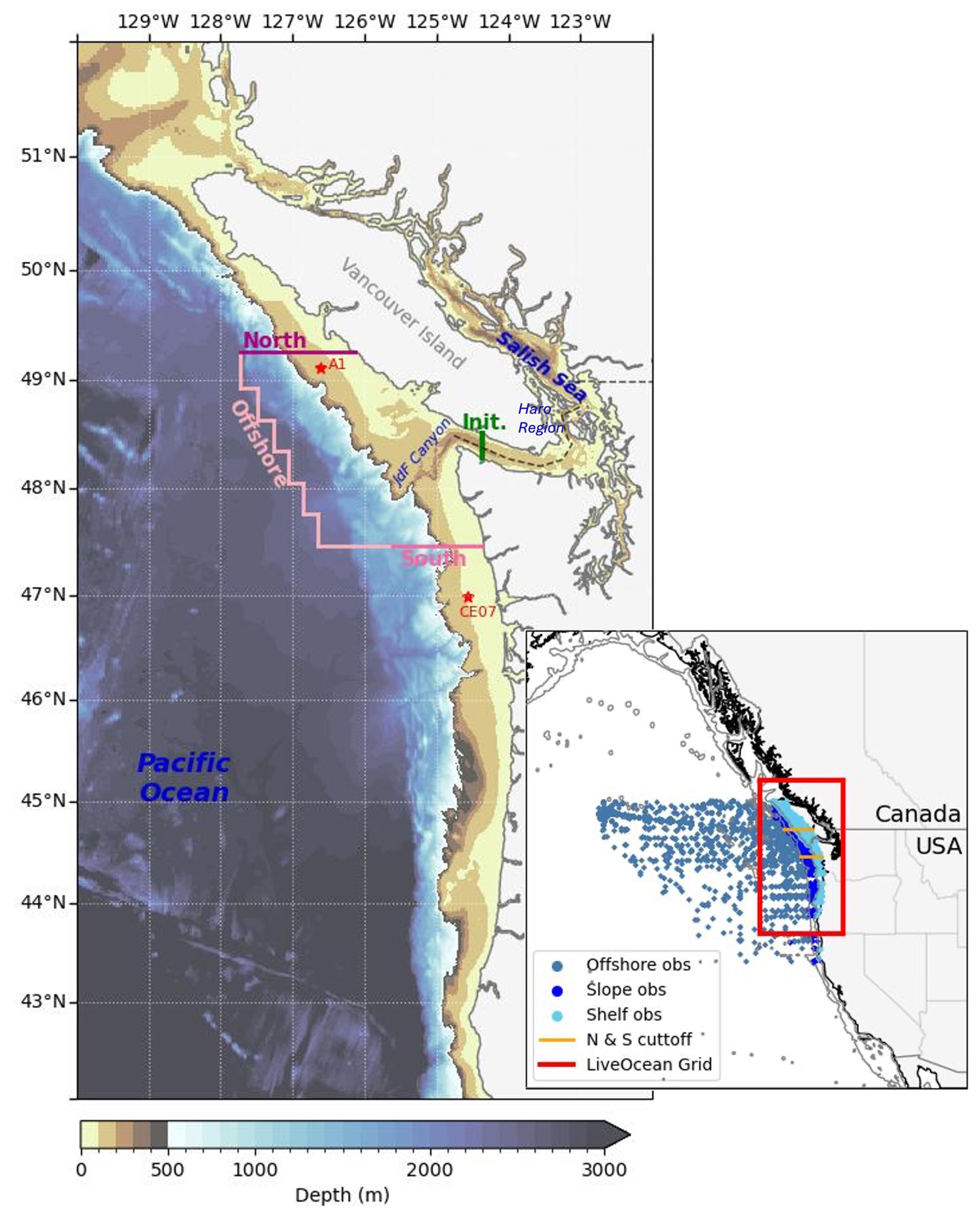
Figure 1 Map of the the LiveOcean domain with bathymetry. The Salish Sea is located along the coast of British Columbia and Washington (the division between Canada and United States, ∼49° N, is shown by a dashed black line in the main map), and is enclosed by Vancouver Island. The simulation initialization boundary, inland of the mouth of JdF, is shown by a green line, while the domain boundaries (North, Offshore, and South) are shown in pink. The location of moorings employed to determine the upwelling and downwelling run-dates (A1 and CE07) are highlighted by red stars. The inset map shows the boundaries of LiveOcean (red box) in the larger context of the Northeast Pacific Ocean. Observations used for source water definitions are divided based on 200 and 2000 m isobars, in grey, with the offshore, slope, and shelf observations in differing shades of blue. The cutoff between the north and south areas of analysis are shown with orange lines over the shelf and slope (Table 1).

The model grid follows lines of constant longitude and latitude, with a horizontal resolution of approximately 500 m in most of the Salish Sea and along the Washington coast. Resolution gradually decreases to 1500 m in the northern Strait of Georgia and 3000 m near the open boundaries, the lowest resolution in the boundaries of analysis in this study is 1650 m (Fig. 1). Vertically, the model is divided into 30σ layers, with a higher density of layers near the surface and bottom.

The conditions of all three open boundaries are based upon fields from the global HYCOM model (Metzger et al., 2014), with daily velocities, temperature, salinity, and sea surface height (ssh) smoothed to remove inertial oscillations. Biogeochemical variables at the open boundaries are specified, using regressions against salinity, derived from cruise measurements (Feely et al., 2016). Tides along these boundaries are forced using eight tidal components (K1, O1, P1, Q1, M2, S2, N2, and K2) from TPXO 9 (Egbert and Erofeeva, 2002). The model's bathymetry incorporates products described in Finlayson (2010) for Puget Sound, Sutherland et al. (2011) for the remainder of the Salish Sea, and Tozer et al. (2019) for the remainder of the model area, all smoothed for stability (Giddings et al., 2014). Daily average gauged flow from the United States Geographical Survey (USGS) and Environment Canada are used to force rivers. For ungauged watersheds, flow estimates are derived from nearby gauged rivers using scaling factors from Mohamedali et al. (2011). Tracer flux from rivers is specified based on local climatology (Xiong et al., 2025). Atmospheric forcings are from output of a Weather Research and Forecasting (WRF) model run by Dr. Cliff Mass at UW (Mass et al., 2003), with a resolution of 1.4 km within most of the LiveOcean domain, 4.2 km north of 49° N or west of 126° W, and 12.5 km north of 50° N.

The updated iteration of LiveOcean performed well in evaluations along the shelf and slope from 2014 to 2018 as detailed in Xiong et al. (2025) and summarized here. In Supplement Sect. S1 we conduct separate evaluations for the subregions of the model, as defined in Table 1. Modelled water properties were compared to data from the Washington Department of Ecology, Department of Fisheries and Oceans (DFO), and National Centers for Environmental Information (NCEI). Water below 20 m had a RMSE (bias) of 0.3 (−0.1) g kg⁻¹ for absolute salinity (S_A), 0.7 (0.0) °C for conservative temperature, 1.1 (−0.2) mg L⁻¹ for dissolved oxygen (DO), 5.0 (0.0) mmol m⁻³ for NO₃, 1.6 (0.8) mmol m⁻³ for NH₄, 47.4 (13.5) mmol m⁻³ for DIC, and 25.5 (−2.7) mmol m⁻³ for TA (Xiong et al., 2025). The high bias and RMSE of NH₄ relative to its range in the region (0–8 mmol m⁻³) led to its removal from model analysis in this paper. Subregion evaluations (Sect. S1) revealed some differences in the bias among regions; notably, deep source waters exhibit a smaller bias in all properties compared to the shallow source waters, and northern waters overestimate DO while all other regions underestimate it.

3.2 Lagrangian Tracking with Ariane

Lagrangian ocean analysis tracks the movement of free-moving entities to estimate ocean pathways by applying the Lagrangian lens of fluid dynamics (Bennett, 2006). Using time-varying velocity, and tracer fields from an ocean model, virtual particles can be simulated to behave like objects (e.g., Van Sebille et al., 2018), zooplankton (e.g., Brasseale et al., 2019), environmental DNA (e.g., Xiong et al., 2025), and pollutants (e.g., Sayol et al., 2014). In this study, the particles are simply neutrally buoyant parcels of water, their paths and transports serve as proxies for dynamics (e.g., Hailegeorgis et al., 2021). Particles can be tracked backwards in time, allowing for source water analysis while avoiding biases inherent in seeding particles from an expected source direction (e.g., Brasseale and MacCready, 2025; Chouksey et al., 2022; de Boisséson et al., 2012).

Ariane is an offline Lagrangian tracking algorithm that assumes time-varying velocity changes linearly between opposite cell faces, preserving local three-dimensional non-divergence in the flow (Van Sebille et al., 2018; Blanke and Raynaud, 1997). This assumption means subgrid-scale mixing is not directly included within Ariane but is parameterized within the underlying numerical model (LiveOcean). Large turbulent eddies are resolved in SalishSeaCast, a 500 m resolution model of the Salish Sea that uses LiveOcean output in its JdF boundary, such that the lack of explicit subgrid-scale mixing does not significantly alter or slow transport, even in mixing hot-spots (Allen et al., 2025; Stevens et al., 2021). Given LiveOcean's high resolution in the model domain, particularly in higher mixing areas near the entrance to JdF, similarly low impact is expected for the simulations in this study. The exclusion of subgrid-scale mixing enables repeatable runs and backwards tracking in Ariane simulations, meaning that multiple experiments over the same domain and time will have the same results (Van Sebille et al., 2018; Blanke and Raynaud, 1997). Ariane supports two analysis modes: qualitative, which tracks individual parcel trajectories, and quantitative, which seeds more particles to enable volume transport analysis without saving individual trajectories. This study employed backward tracking in the quantitative mode.

In the quantitative mode, parcels are seeded along an “initialization” section (green boundary in Fig. 1) and tracked until they reach simulation boundaries (pink boundaries in Fig. 1) or pass back over the initialization section (hereafter referred to as loop(ed) parcels) (Blanke et al., 2001). The initialization and simulation boundaries are distinct from model boundaries, they are user-defined and must follow the model grid (i.e. they cannot cut diagonally across cells). Parcels that never reach a boundary within the analysis period are classified as “lost”. Parcels are distributed across the initialization section at each time-step proportional to the transport (where transport through a cell q is equal to the velocity through a cell multiplied by its area, $q=u\times A$) in each model grid cell where the direction of transport is towards the analysis domain (westward in Fig. 1). Time-step here refers to the particle tracking time-step within Ariane, which does not need to be the same as the model output time-step, but in the case of this study are the both one hour. The number of parcels seeded, n per cell, is determined by dividing q by the user-defined maximum transport per parcel q_max ($n=q/q_{\max }$, rounded up to the integer). Parcels are evenly distributed within the cell, and their constant volume flux V_n (m³ s⁻¹) is defined as $V_n=q/n$.

Lagrangian particle simulations were conducted from 2014 to 2023 (inclusive), with separate runs for each upwelling, downwelling, spring transition, and fall transition period (as defined in Sect. 3.5). Particles were continuously released over the analysis period, with each run including an additional 100 d without particle seeding to allow particles sufficient time to travel between boundaries based on histograms of crossing times in Beutel and Allen (2024) and checked again in this study (Fig. S8). Six tracers from LiveOcean were input into the simulations: S_A, temperature, DO, NO₃, DIC, and TA; necessitating three runs per analysis period as only two tracers can be input into Ariane at a time. It should be noted that [TA-DIC] was used to study carbonate chemistry in JdF inflow, as opposed to TA and DIC individually, as the difference between the two terms can be used more effectively to investigate ocean acidification (OA; Xue and Cai, 2020); a large positive [TA-DIC] indicates a high buffering capacity with respect to OA, while low or negative values indicate that the region is vulnerable to OA.

Looped parcels that pass back over the initialization section within 24 h of seeding (two tidal cycles) are considered “tidally pumped” parcels and are removed from analysis, the remaining looped parcels can be thought of as reflux circulation through JdF (MacCready et al., 2021). The transport estimates in this study are based on parcels that complete a full trajectory – from initialization either to the shelf or offshore boundaries, or return to the initialization section. Water that is already within the analysis domain (lost parcels, representing ∼ 1 % of seeded parcels) or tidally pumped water (representing ∼ 72 % of seeded parcels) are excluded from these estimates. As a result, the reported volumes should not be interpreted as estimates of total transport through JdF; doing so would result in a substantial underestimate (Beutel and Allen, 2024).

Beyond lost and looped parcels, sources were assigned based on parcel position and salinity at the point they crossed a boundary (Table 1). The analysis boundaries follow those defined in Beutel and Allen (2024): the initialization section, south, north, and offshore, with salinity and depth thresholds redefined for LiveOcean output (Sect. S2). The location of the initialization section is set inland of the mouth of JdF to reflect waters that actually reach the sea's inner basins, or at least do to the degree found in Beutel and Allen (2024). Despite the extension of the northern boundary to near the 2000 m isobath, water parcels originating along that boundary are defined as shallow as they predominantly (85 % of transport) intersect the boundary at depths shallower than 200 m. While south brackish water is expected to originate from the Columbia River plume (Hickey et al., 2009), evaluating the dominance of that source on brackish flow from the south is outside of the domain and scope of this study; other small rivers along the coast may contribute to this source. Offshore water is divided into surface and deep source waters based on the approximate offshore mixed-layer depth (Sect. S2.2).

Table 1 Source water definitions for the particle tracking simulation (a) and the division of observations (b) . The boundaries for particle tracking definitions refer to those shown in Fig. 1. The regions (offshore, slope, shelf) of observations are defined by their location relative to bathymetric contours, offshore is oceanward of 2000 m, shelf is shoreward of 200 m, and slope is between the two. Note that no observations exceeding depths of 500 m were used.

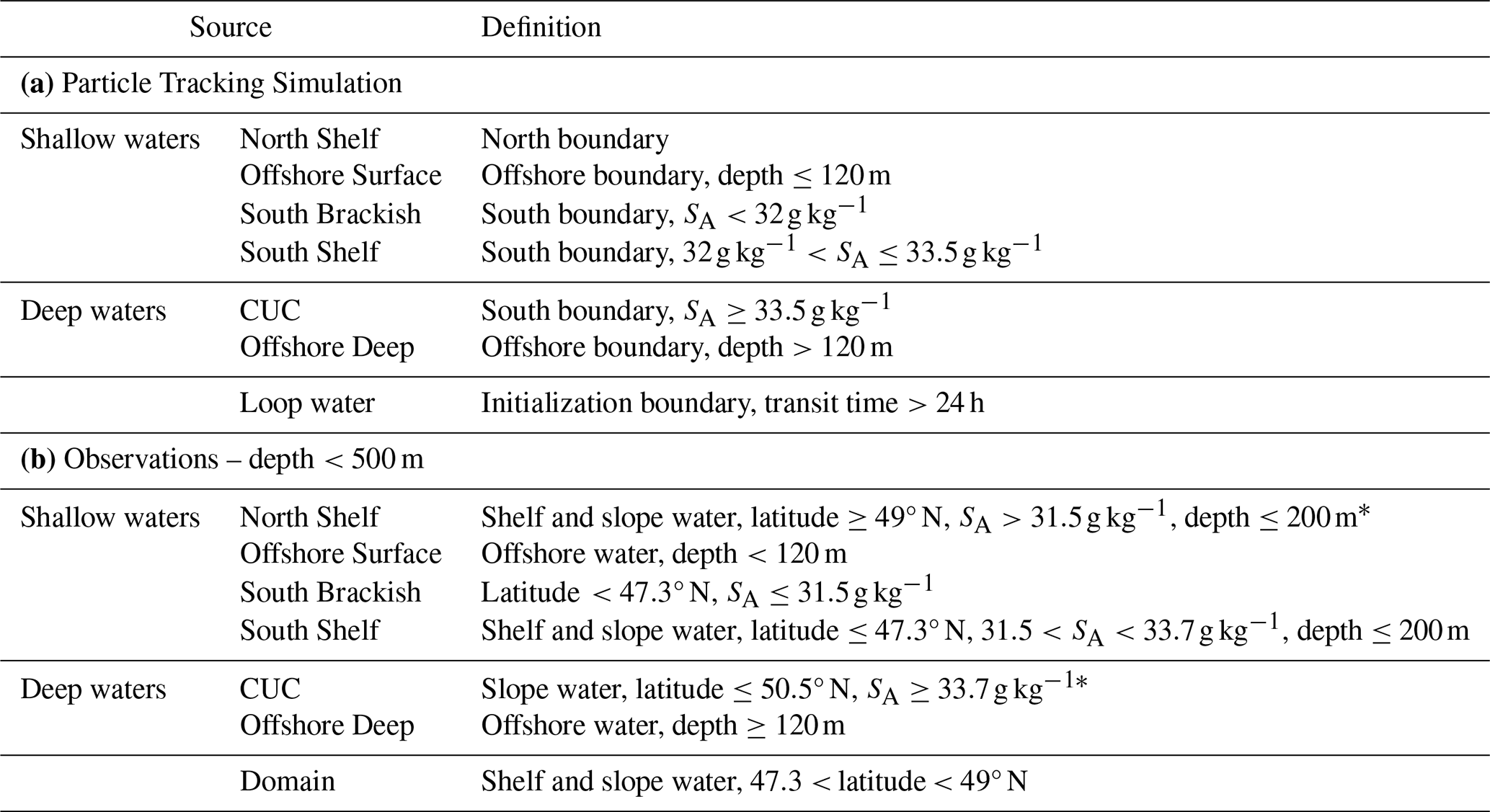
^* All observations north of 49^∘ N and shallower than 200 m were less saline than 33.7 g kg⁻¹, as such the CUC and North water observation definitions do not overlap.

3.3 Attribution of Interannual Variability Drivers

The volume flux of a property (PJ) into JdF is calculated as the sum of contributions from each water source (i):

$$\begin{array}{}\text{(1)}& PJ=\sum P_i{J}_i\end{array}$$

Here, P represents the mean property value in the JdF inflow, and J (m³) is the total volume of water over the analysis period (i.e., the volumetric flow rate (m³ s⁻¹) multiplied by the period length (s), J=Qt). For each water source i, P_i and J_i denote the mean property value and the volume contribution, respectively. To analyze the drivers of changes in the flux of properties into JdF (Δ(PJ)) over time, variations in annual volume and properties are decomposed (Sect. S4) into components driven by changes in dynamics ($\mathrm{\Delta }{J}_i=J_i^{\mathrm{year}}-J_i^{\mathrm{base}}$), changes in properties ($\mathrm{\Delta }{P}_i=P_i^{\mathrm{year}}-P_i^{\mathrm{base}}$), and correlated changes (ΔP_iΔJ_i):

$$\begin{array}{}\text{(2)}& \mathrm{\Delta }\left(PJ\right)=\sum (\mathrm{\Delta }{P}_i{J}_i^{\mathrm{base}}+P_i^{\mathrm{base}}\mathrm{\Delta }{J}_i+\mathrm{\Delta }{P}_i\mathrm{\Delta }{J}_i)\end{array}$$

Baseline values ($J_i^{\mathrm{base}}$ and $P_i^{\mathrm{base}}$) are defined as the mean volume flux and mean property value of each water mass, computed for periods of upwelling, downwelling, or the combined downwelling and subsequent upwelling season over the ten years of analysis. Contributions to variability are normalized by Δ(PJ) such that Eq. (2) sums to 1, so that the difference in importance of property and volume driven variability between tracers and years can be easily compared. Annual values ($J_i^{\mathrm{year}}$ and $P_i^{\mathrm{year}}$) reported in this paper are computed for a combined downwelling, spring transition, upwelling, and fall transition.

In this study, all of the inputs into Eq. (2) are derived from the Lagrangian simulations. Values for $J_i^{\mathrm{year}}$ are the sum of water parcel volumes from a water source over a year and values for $P_i^{\mathrm{year}}$ are the volume weighted mean properties from a source over that same period. Where observations are available within each water source with sufficient spatial and temporal coverage to assess variation with confidence, it is possible to combine observed mean P_i with simulated J_i. This application of Eq. (2) was not examined in this paper, but is an interesting potential application for future study in areas such as the Newport Hydrographic Line (NHL) where observations are collected biweekly (Risien et al., 2022).

While interannual variation is the most straightforward application of Eq. (2), the analysis is flexible, such that other modes of variation can be calculated. Division of water parcels within each source by density ranges, as opposed to years, is also applied in this paper to assess the contribution of each water source to variability within an isopycnal range over the ten analysis years. Little changes in the equation, J_base and P_base are unchanged; ΔJ_i and ΔP_i become $\mathrm{\Delta }{J}_i=J_i^{{\mathit{\sigma }}_{\mathrm{1}}-{\mathit{\sigma }}_{\mathrm{2}}}-J_i^{\mathrm{base}}$ and $\mathrm{\Delta }{P}_i=P_i^{{\mathit{\sigma }}_{\mathrm{1}}-{\mathit{\sigma }}_{\mathrm{2}}}-P_i^{\mathrm{base}}$, where σ₁−σ₂ signify a particular isopycnal range.

3.4 Observed Tracers

Observations are used in this study to extend the discussion of the drivers of biogeochemical variability beyond tracers available in LiveOcean. Tracers that exist in both the model (Sect. 3.1) and the collated observations are used as tools to qualitatively connect un-modelled tracers to the variability and attribution results in this study. Observations on and offshore of the British Columbia (BC), Washington, and Oregon coasts were collated from nine sources (Table A1). These datasets span a wide range of time (1930 to the end of 2023), spatial coverage, and measurement techniques, including cruise-based bottle and/or conductivity temperature depth (CTD) profiles as well as CTD-mounted moorings.

To reduce the computational load for large datasets with unnecessarily high resolutions (e.g., moorings with minute-by-minute measurements), datasets were binned into day-averages at 1 m depth intervals. Outliers were removed by excluding data points that lay more than four standard deviations from the variable's mean at a particular depth. An exception was made for S_A, where values far below the mean but greater than zero were retained to preserve freshwater measurements. Observations of density, spiciness (McDougall and Krzysik, 2015; Pawlowicz et al., 2012), and N^* (a combination of NO₃ and dissolved inorganic phosphorus (DIP) used to investigate nitrification/denitrification; Gruber and Sarmiento, 1997) were calculated where the required parameters were available.

After combining datasets, duplicates were identified and removed based on latitude (to two decimal places), longitude (to two decimal places), time (to the day), and depth (1 m bins). Duplicate observations were combined by taking the mean of the measurements. To encompass the northern CCS, only observations shallower than 500 m, within 1000 km of the coast (Hickey, 1979), and between 40 and 50.8° N were kept (Checkley and Barth, 2009). While deep source waters may influence the Salish Sea via upwelling onto the shelf or through the Juan de Fuca Canyon, upwelled water originates from depths shallower than 500 m with the bulk from depths less than 150 m (Beutel and Allen, 2024; Bograd et al., 2001).

Observations were categorized as offshore, slope, or shelf based on the bathymetry of the observation sites (Fig. 1). Offshore observations were defined as those seaward of the 2000 m isobath, shelf as those landward of the 200 m isobath, and slope as those between these two boundaries. Further division into source waters (north shelf, offshore surface, south brackish, south shelf, CUC, offshore deep, and domain; Table 1) was based on trajectories identified in this study (Sect. 4.1) and Beutel and Allen (2024), and property-property diagrams of temperature, S_A, NO₃, and TA. The sensitivity of the source classifications to these criteria is discussed in Sect. S2.

3.5 Upwelling and Downwelling Timing

Upwelling and downwelling were divided in some of the analysis in this study to identify the impact of seasonality, but most analysis was conducted over a full year. Please note that when the text refers to annual values it does not mean one calendar year, instead a year in this paper refers to the combination of one set of consecutive downwelling, spring transition, upwelling, and fall transition periods, all of which differ in length interannually. A combination of upwelling estimates were used to identify the length of these periods: meridional velocity measurements at moorings A1 and CE07 (Fig. 1; maintained by the DFO and the Ocean Observatories Initiative (OOI), and available from 2013–2020 and 2015–present, respectively), spring and fall transition timing (upwelling highlighted by yellow bars in Fig. 2b; Hourston and Thomson, 2024, available from 1980–present), and the Bakun Index at 48° N (upwelling highlighted by grey bars in Fig. 2b; Bograd et al., 2009; Bakun, 1973, available from 1967–present). Upwelling and downwelling timing (red and blue in Fig. 2a, respectively) was determined by the overlap of these measures, with non-overlapping periods designated as transition intervals (white in Fig. 2a). If this method produced buffer periods shorter than 20 d (Lynn et al., 2003), or if only one upwelling estimate was available (observations predating estimates in Hourston and Thomson, 2024), the bounding upwelling and downwelling periods were shortened to ensure a minimum transition length of 20 d. For periods predating the Bakun Index (before 1967), upwelling and downwelling periods were conservatively set to May–August (inclusive) and November–February (inclusive), respectively.

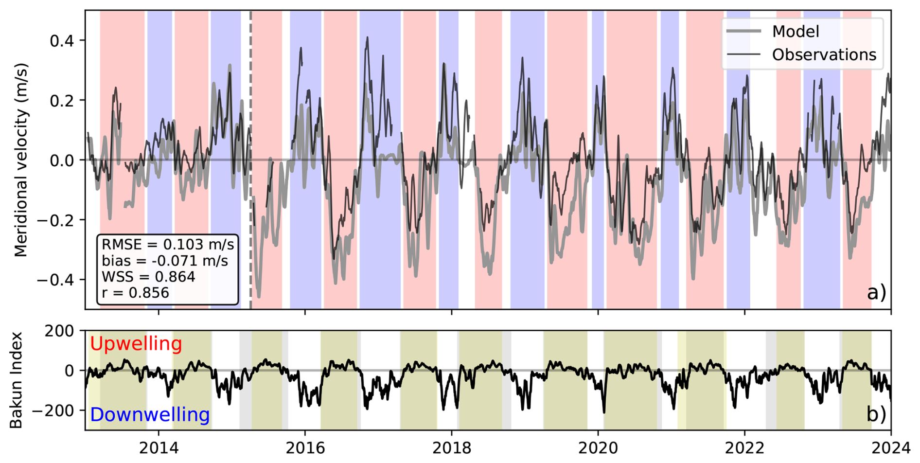
Figure 2 Date selection for upwelling (red) and downwelling (blue) periods between 2013 and 2024. Modelled and observed alongshore velocity (a) at station A1 before April 2015 (vertical black dashed line) and CE07 after, smoothed using a 15 d running mean as in Foreman et al. (2011). White areas between upwelling and downwelling indicate periods of transition between the two regimes. The Bakun index (b) estimates the strength and direction of vertical Ekman transport near the coast, with a positive Bakun index meaning upward transport (ie. upwelling). Periods of upwelling as defined by the Bakun index (grey) correlate well with those outlined in Hourston and Thomson (2024) (yellow).

The Bakun Index is based on local wind stress (Bakun, 1973); however, upwelling timing in the Northern California Current System may be influenced by remote winds as far south as 36° N (Engida et al., 2016), where upwelling favourable winds occur year round (Bakun, 1973). To test the sensitivity of results to the Bakun Index latitude, date selection was repeated using the Bakun index at 45° N. In general the dates were in close agreement, with upwelling and downwelling dates differing by a week or less in most cases. However, in 2013, upwelling timing differed significantly, starting 18 d later and ending 33 d earlier when using the Bakun Index at 45° N instead of 48° N. This discrepancy was unexpected, as upwelling further south typically begins earlier and lasts longer than at higher latitude. Due to this inconsistency and the otherwise similar results between the two Bakun index latitudes, the Bakun index at 48° N (along with the Hourston and Thomson, 2024 dates and the modelled and observed alongshore velocity at A1 and CE07) were deemed a reasonable choice for defining seasonal upwelling and downwelling periods in this region.

4 Results

4.1 Salish Sea Inflow

In general, loop water (return flow from JdF) accounts for the most JdF inflow in a given year at 30.7 % of inflow or averaging $(\mathrm{4.3}\pm \mathrm{0.4})\times {\mathrm{10}}^{\mathrm{8}}{\mathrm{m}}^{\mathrm{3}}$ (Fig. 3b); the volume flux of loop water remains relatively consistent throughout the year, though it accounts for a larger portion of inflow during downwelling. Loop water is made up of a varying mixture of the Pacific sources and of river discharge originating in the Salish Sea. As such, while its contribution to inflow volume and interannual property and dynamical variability is important (Sect. S3), it should not be treated as an unique or separable source from the other analyzed source waters. Instead, the dynamics and properties of loop water should be thought of as another product of JdF inflow variability partially driven by the Pacific sources. The remainder of this paper will focus on the Pacific sources of flow into JdF (i.e. parcels originating from one of the outer, pink, boundaries in Fig. 1).

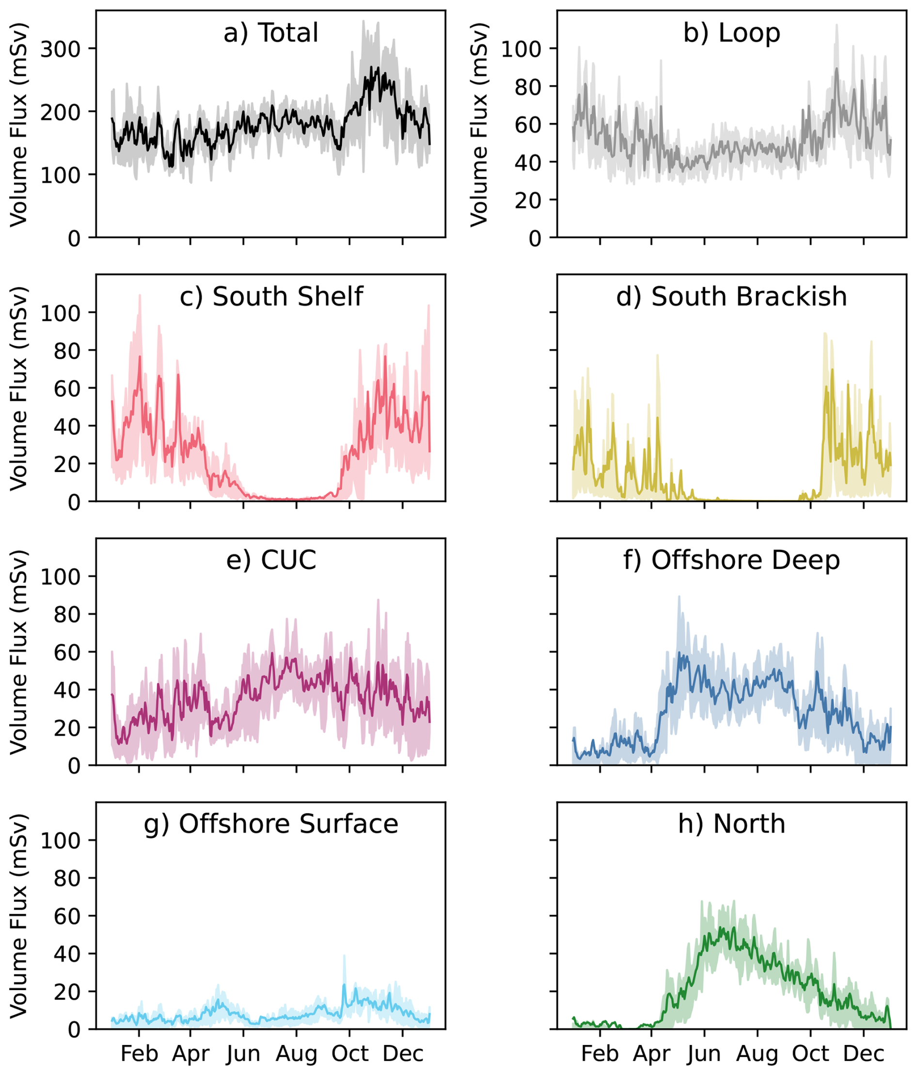
Figure 3 Daily average modelled transport (1 mSv =10³ m³ s${}^{-\mathrm{1}}=\mathrm{8.64}\times {\mathrm{10}}^{\mathrm{7}}$ m³ d⁻¹) into JdF (a) and from each source water (b–h) averaged for the same year-day (solid line) with the inter-quartile ranges about the mean shown in a lighter shade. Note that the vertical range of (a) is about three times as large as those from the individual water masses (b–h). Months May–September are typically periods of upwelling, while months November–March are typically periods of downwelling.

The water reaching JdF from the Pacific largely originates between potential density surfaces (σ₀) of 25.4–26.5 kg m⁻³ (based on the first and third transport-weighted quartiles of JdF inflow), aligning with the density of the inflow layer at the initialization section (Fig. 4a). The CUC is the largest Pacific source, with $(\mathrm{2.8}\pm \mathrm{0.4})\times {\mathrm{10}}^{\mathrm{8}}{\mathrm{m}}^{\mathrm{3}}$ of inflow annually (Fig. 5a) and a mean σ₀ of 26.5 kg m⁻³ (Fig. 4b), contributing significantly to JdF inflow throughout the year (Fig. 3e). Offshore deep water is predominantly an upwelling source (Fig. 3f), with $(\mathrm{2.1}\pm \mathrm{0.4})\times {\mathrm{10}}^{\mathrm{8}}{\mathrm{m}}^{\mathrm{3}}$ annually and a mean σ₀ of 26.4 kg m⁻³. Offshore surface water enters JdF in small amounts year round (Fig. 3g), totalling $(\mathrm{0.6}\pm \mathrm{0.2})\times {\mathrm{10}}^{\mathrm{8}}{\mathrm{m}}^{\mathrm{3}}$ annually with a mean σ₀ of 25.3 kg m⁻³. North water reaches JdF almost exclusively during upwelling (Fig. 3h), with $(\mathrm{1.5}\pm \mathrm{0.2})\times {\mathrm{10}}^{\mathrm{8}}{\mathrm{m}}^{\mathrm{3}}$ annually on a mean σ₀ of 25.8 kg m⁻³, while south brackish water reaches JdF almost exclusively during downwelling (Fig. 3d), with $(\mathrm{0.9}\pm \mathrm{0.2})\times {\mathrm{10}}^{\mathrm{8}}{\mathrm{m}}^{\mathrm{3}}$ annually along a much shallower mean σ₀ of 23.0 kg m⁻³. South shelf water is predominantly a downwelling source, with $(\mathrm{1.8}\pm \mathrm{0.4})\times {\mathrm{10}}^{\mathrm{8}}{\mathrm{m}}^{\mathrm{3}}$ and a mean σ₀ of 25.2 kg m⁻³; of the six source waters it had the highest standard deviation in annual inflow (Fig. 3c). The timing and dominance of source waters align well with those in Beutel and Allen (2024). Significant mixing occurs between the analysis boundaries and the initialization section, such that once reaching JdF the water sources fall within similar isopycnal ranges with the exception of south brackish water (Fig. 4c).

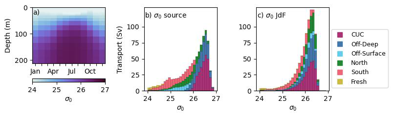
Figure 4 Water source contributions to JdF inflow in isopycnal space. Mean monthly density anomaly (a) at the centre of the initialization transect (Fig. 1) according to SalishSeaCast output from 2007–2023 (Allen et al., 2025). Histograms of transport weighted density anomaly of water parcels at their location of origin (b) and at the initialization transect (c). Histograms of transport weighted parcel depth at the beginning and end of transit are available in Fig. S9.

As is the case with any continuous process, it should be noted that the dynamics of a given year will be impacted by the one preceding it. Typical parcel advection time differs between source waters (Fig. S8), ranging between 8 d for south brackish water and 60 d for offshore deep water. As such, some slower advecting source waters may be brought into the vicinity of JdF during a preceding period. For example, it is possible that parcels originating from the CUC at the beginning of downwelling or the fall transition were actually brought onto the shelf during upwelling (note the slightly higher contribution of CUC water in November and December than in January and February, Fig. 3e).

The length (Figs. 2b and 5b) and strength of upwelling and downwelling periods results in significant year-to-year differences in the water entering the Salish Sea (Figs. 5, S10). The inflows of south shelf and brackish water have a significant (significance level (α)=0.05) correlation with the difference in length of consecutive upwelling and downwelling periods (Fig. 5b), the correlation coefficient $\left(r\right)=-\mathrm{0.81}(p=\mathrm{0.005})$ and $-\mathrm{0.75}(p=\mathrm{0.01})$, respectively, while north shelf water is significantly correlated with the strength of upwelling, r=0.72 (p=0.02). For instance, in 2017, the downwelling season lasted longer than upwelling and the inflow of south shelf and brackish water was higher than typical. In 2020, despite upwelling lasting for a significant amount of time north water inflow volumes were low, owing potentially to the relative weakness of this upwelling period (Fig. 2b). The interannual variability in season length and source water contribution also manifests in the JdF inflow properties (Fig. 5c–g). The mean S_A, DO, and NO₃ of JdF inflow are significantly correlated to the difference in upwelling and downwelling length, with r=0.68 (p=0.03), −0.72 (p=0.02), and 0.66 (p=0.04), respectively. It should be noted that density varies strongly with salinity in the region (r=0.9, p=0.001); only interannual salinity variability is shown but a density comparison is available in Fig. S10.

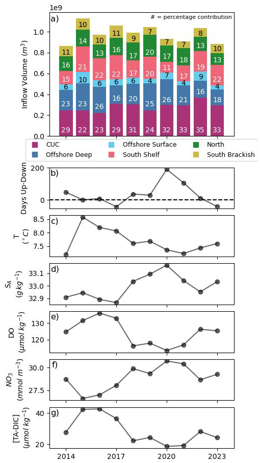
Figure 5 (a) Volume from the CUC (purple), offshore deep (navy), offshore surface (light blue), south (pink), north (green), and brackish (yellow) water into the Salish Sea over one year (combined periods of downwelling, spring transition, upwelling, and fall transition). The percentage contribution to JdF inflow from each water source over a year is overlaid on each bar. A version of (a) including the contribution of loop water is included in Sect. S3. (b) Difference in the length of upwelling and downwelling in each year. Variability in the modelled transport weighted mean temperature (c), S_A (d), DO (e), NO₃ (f), and [TA-DIC] (g) of water parcels at the mouth of JdF may relate to the flux from each source water. Transport weighted mean density correlates very strongly with salinity (Fig. S10).

4.2 Source Water Properties

4.2.1 Observed Properties

The separation of observations into source waters (Table 1) highlights distinct differences between deep (offshore deep and CUC water) and shallow source waters (north and south shelf water, and offshore surface water; Fig. 6). Deep source waters are colder, saltier, and denser than shallow waters. They are also richer in nutrients, DIC, and TA, while being lower in DO and ${\mathrm{CO}}_{\mathrm{3}}^{\mathrm{2}-}$ concentrations. Denitrification (negative N^*) is more prevalent than nitrification across all source waters, thus the mean N^* are all negative, ranging from −1.8 in offshore deep to −3.8 in the south shelf water (Table A3). In Fig. 6, a high N^* refers to a less negative N^*, and it is associated with the deep source waters, consistent with their higher concentrations of NO₃ and DIP and lower concentrations of the denitrification precursor (NH₄).

The two deep source waters (CUC and offshore deep) are surprisingly similar, differences in their properties are often not statistically significant (based on a 95 % confidence interval p-test, Table A3) or, where they are statistically significant due to abundant observations, are not practically different (as indicated by a Cohen's d<0.5 (Cohen, 1988), suggesting small effect size). Notable exceptions are that the CUC is warmer, spicier, and richer in NO₂ than offshore deep water. These similarities persist in time and north-south location (based on 1° latitude binning), but some differences in the properties of the two water sources with depth are present. Between 100 and 300 m the CUC and offshore deep water diverge more in many biologically influenced properties (DO, NO₃, NO₂, DIP, dissolved silicon (DSi), TA). This result may suggest that the CUC and offshore deep sources are made up of similar water mass mixtures, but that more respiration occurs in one source, the CUC in this case. Shallow source waters differ more-so: offshore surface water is more oxygen rich and has significantly higher aragonite and calcite saturation than shelf source waters. Among shelf waters, north shelf water is less spicy, while south shelf water exhibits a higher TA.

Seasonal differences are more pronounced in shallow source waters, while deep source waters remain relatively consistent across upwelling and downwelling periods (Fig. 6). These seasonal variations also reveal greater distinctions between shallow source waters. For example, NO₃ and DIP concentrations are higher in south shelf water in the summer due to upwelling but higher in offshore surface water during downwelling due to winter mixing, with little variation in north shelf water (Fig. 6).

Trace metal observations are scarce with the exception of the offshore source waters (Table A2). Available data suggest that the CUC has higher concentrations of Co, Fe, and Mn than offshore deep water, even though these source waters are otherwise similar (Fig. 6). Offshore surface water generally has lower trace metal concentrations compared to offshore deep water, except for Mn. The limited trace metal observations of north and south shelf water in particular (three and two measurements, respectively, Table A2) make it such that few significant differences exist between these sources and the others (Table A3). The Cd, Mn, and Fe concentrations in north shelf water stand out as high compared to the other surface water masses, and in the case of Cd and Fe, align more closely with the deep water masses.

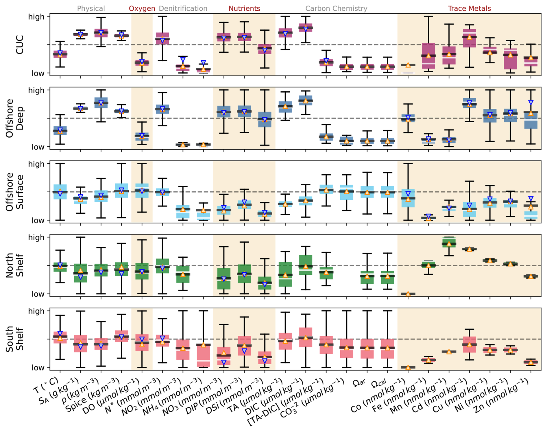
Figure 6 Relative property definitions of each source water (Table 1) based on observations (Fig. 1-inset). High and low limits are relative to the other source waters, based on the maximum and minimum whisker values among the five source waters in each property. The light grey line within each box indicates the median value, the upward pointing orange triangle represents the mean over upwelling periods, and the downward pointing blue triangle the mean over downwelling periods (where downwelling observations were available, Table A2). The observed tracer mean and standard deviation in each source water, and the significance of differences between source waters, is summarized in Table A3.

4.2.2 Modelled Properties

Given the inconsistent sampling frequency and locations, interannual variability in source water biogeochemistry is difficult to assess from observations alone. To supplement this analysis, modelled variability in annual transport weighted mean source water properties (Fig. 7) was evaluated. Comparisons between model and observational data (Sect. S1) confirm that the model accurately represents the range and variability of properties. Across the domain, modelled S_A, temperature, DO, NO₃, TA, and DIC show high skill (Willmott Skill Scores (WSSs) ≧0.90, Willmott, 1981). Subregion (as defined in Table 1, observations) evaluations yield slightly lower skill for some tracers, notably TA in offshore surface water (WSS =0.76), but all other tracers in all subregions achieve WSSs ≧0.81.

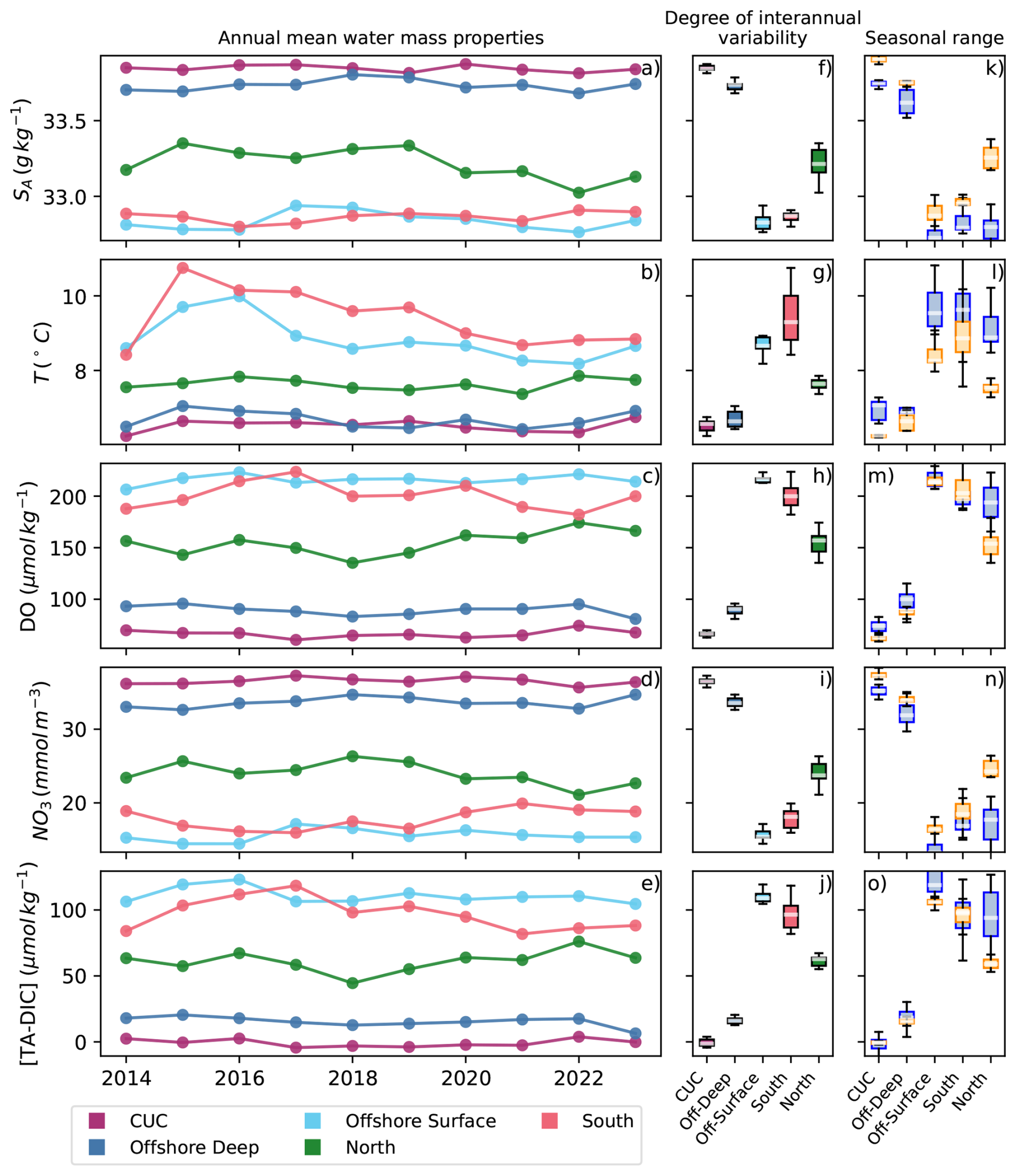
Figure 7 Modelled properties and their interannual (a–j) and seasonal (k–o) variability. Transport weighted annual mean (a–e) S_A, temperature, DO, NO₃, and [TA-DIC] at the outer boundaries for the CUC (purple), offshore deep (blue), offshore surface (light blue), north (green), and south (pink) source waters. Box and whisker plots (f–j) of the combined annual data show the range in properties exhibited by each source water. Box and whisker plots of upwelling (orange) and downwelling (blue) properties (k–o) show the seasonal difference in source water properties in each source water.

In general, shallow source waters (south shelf, loop, offshore surface, and north water) exhibit more interannual variability over the analysis period than deep source waters (CUC and offshore deep water, Fig. 7). Temperature change in particular seems to manifest in the shallow source waters, with the elevated water temperatures in the northeast Pacific during the 2014–2016 marine heatwave (the “Blob”, Bond et al., 2015) clearly present in the south shelf, offshore surface, and loop water (Fig. 7b). South shelf water has among the most interannual variability in each water property, with north shelf water only exceeding it in NO₃ content. Shallow source waters generally have stronger seasonal cycles than the deep source waters. All three shallow sources exhibit the same property changes during upwelling: increased salinity, cooler temperatures, lower DO, and higher concentrations of NO₃, TA, and DIC compared to downwelling periods. This seasonal trend is in opposition to that found for offshore surface water in the observational data, but is aligned for the two shelf water masses (Fig. 6).

Brackish south water, excluded from Fig. 7 due to its distinct property range, is significantly lower in salinity, NO₃, DIC, and TA, and higher in DO than the other source waters. It also appears to be even more impacted by the Blob than the other shallow source, but otherwise overlaps in temperature with the shallow source waters. Focusing only on downwelling periods due to the lack of brackish south water during most upwelling periods, this source water has little interannual variability except in temperature.

4.3 Drivers of Variability

Using Eq. (2), we separated the effects of annual variability in the volume of water contributed by each Pacific source water (Fig. 5a, b) from variability in the properties of those source waters (Figs. 6, 7). The cross term (third term in Eq. 2) is small relative to the impacts of dynamical and property variability, and so is neglected in this analysis. Overall, dynamical variability accounts for the majority of variability in each tracer (Fig. 8). However, property variability plays a substantial role in explaining changes in temperature, DO, and NO₃ ($\sim \frac{\mathrm{1}}{\mathrm{6}}$), and a major role in the variability of [TA-DIC] ($\sim \frac{\mathrm{1}}{\mathrm{4}}$). Notably, in two of the analyzed years (2016 and 2018), property variability plays a larger role than dynamical variability in the change in [TA-DIC] flux. High property driven variability in a given year does not directly align with interannual extremes in said properties. For example, in 2017 the [TA-DIC] concentration in south shelf water is more extreme than it was in 2016; however, property variability from south shelf water is a smaller driver in 2017 because higher than typical transport from shallow water sources overshadow the property impact.

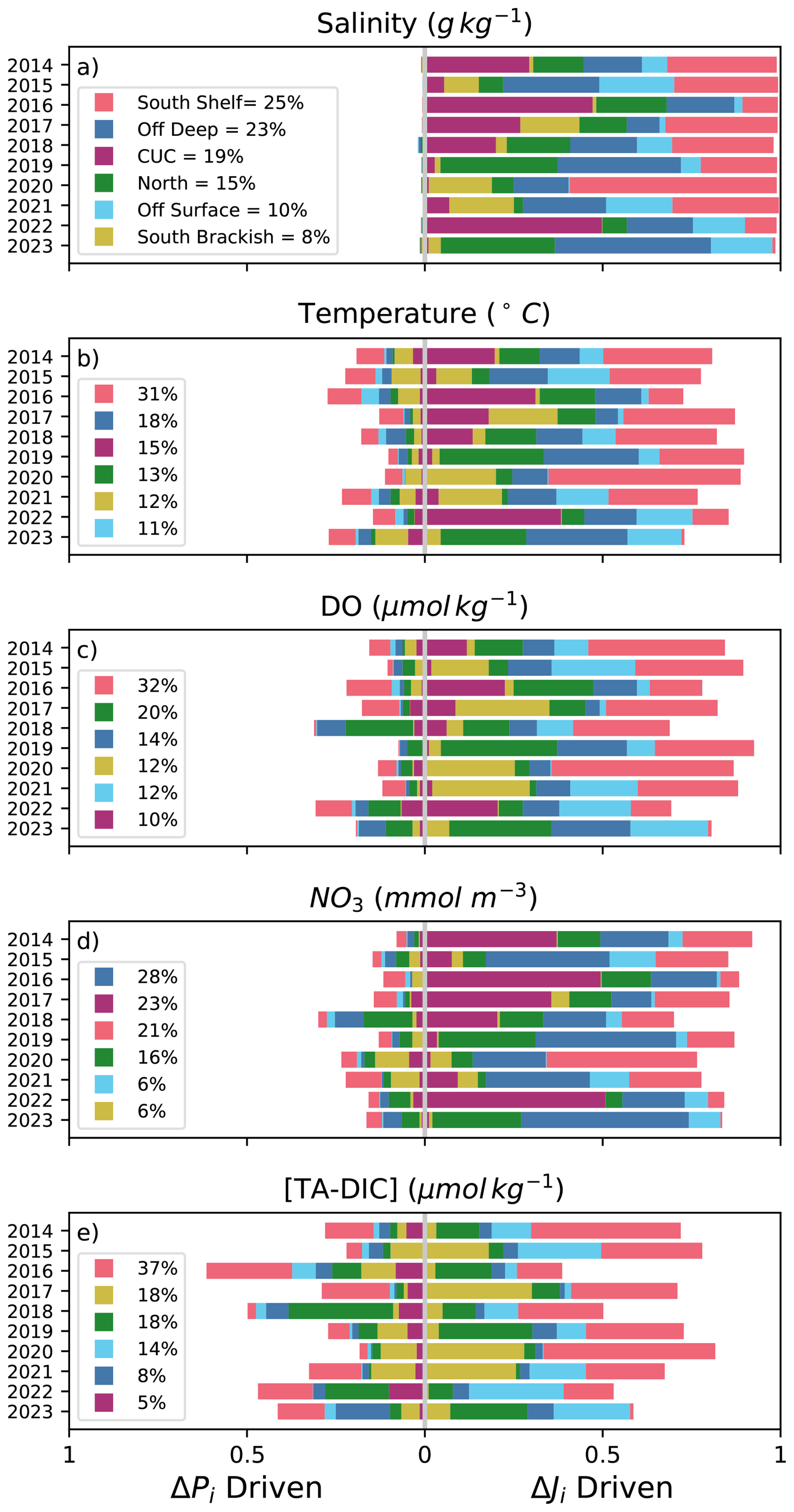
Figure 8 Normalized attribution of changes in Salish Sea inflow flux of S_A (a), temperature (b), DO (c), NO₃ (d), and [TA-DIC] (e) to interannual differences in source water inflow volumes (right side of the graph) or to interannual differences in source water properties (left side). The legend in each figure displays the average percentage contribution of each source water to interannual variability in the tracer over the ten years of analysis, the source waters are reordered in each legend according to their contribution (top to bottom). The Supplement includes versions of this figure for contributions to density variability (Fig. S11), and including the contribution of loop water (Fig. S7).

The source waters that explain the most interannual variability differ from tracer to tracer, and, accordingly, don't correspond with which source waters contribute most to JdF inflow. Offshore deep water and the CUC are the two largest Pacific contributors to Salish inflow (Fig. 5a), but with the exception of NO₃ variability, the contribution of CUC and offshore deep water to interannual variability is smaller than their volume contribution. The deep source waters contribute similar amounts overall to variability, predominantly in the form of dynamical variability (Fig. 8). Despite south shelf water contributing a smaller portion of JdF inflow annually (Fig. 5a) compared to CUC and offshore deep water, it is the largest driver of interannual variability in all but NO₃, where deep waters are more important (Fig. 8d). South shelf water contributes to interannual variability in the form of both dynamical and property variability in large amounts, but dynamical variability plays a larger role. The other shallow source waters (north shelf, brackish south, and offshore surface water) are large drivers of interannual variability in DO and [TA-DIC], with their contributions to variability far exceeding their contributions to inflow volume in those tracers. It should be noted, however, that these contributions to variability are themselves variable: the standard deviation in each source water's contribution exceeds one third of its mean ($\mathit{\sigma }>\frac{\mathrm{1}}{\mathrm{3}}\stackrel{\mathrm{‾}}{x}$), with CUC and south brackish water showing the largest year-to-year fluctuations.

On seasonal scales, the relative importance of water sources to variability shift closer to their volume contributions (Fig. 3; Beutel and Allen, 2024). South shelf and south brackish water are very important to variability during downwelling, and are much smaller sources of variability during upwelling, when the contribution of offshore deep and north shelf water increase substantially (Fig. S12). The CUC is an important contributor to variability year-round.

Reorganizing water source transport into density bins as opposed to an annual grouping reveals which source waters contribute to tracer variability in different isopycnal ranges (Fig. 9). As may be expected, deep water masses primarily contribute to variability in higher isopycnal ranges and shallow water masses contribute more at lower isopycnal ranges. However, this division is an oversimplification. Offshore deep water for example, significantly contributes to variability in a larger isopycnal range than the CUC, and north shelf water contributes significantly to variability over the entire isopycnal range of water reaching JdF, in line with its large range in density (Fig. 4b). Like in the analysis of interannual variability, the difference in water source and driver importance between tracers is striking. The CUC is a large contributor to variability at ${\mathit{\sigma }}_{\mathrm{0}}\ge \mathrm{25.6}\mathrm{kg}{\mathrm{m}}^{-\mathrm{3}}$ in salinity, temperature, and NO₃, but decreases in importance for DO, and is almost negligible at any range for [TA-DIC]. The overall dominance of drivers is the same as in the interannual analysis (Fig. 8), but the density grouping reveals that property driven variability is stronger in all tracers at high (${\mathit{\sigma }}_{\mathrm{0}}\ge \mathrm{26.8}\mathrm{kg}{\mathrm{m}}^{-\mathrm{3}}$) and low (${\mathit{\sigma }}_{\mathrm{0}}\le \mathrm{25.2}\mathrm{kg}{\mathrm{m}}^{-\mathrm{3}}$) isopycnal ranges, while dynamical variability is stronger for intermediate waters.

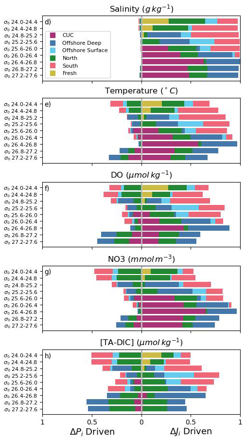
Figure 9 Normalized attribution of changes in Salish Sea inflow flux of S_A (a), temperature (b), DO (c), NO₃ (d), and [TA-DIC] (e) to differences in source water inflow volumes (right side of the graph) or properties (left side) along source isopycnals. Note that the total transport in each isopycnal range is not equal (Fig. 4b).

The significant mixing of source waters at the entrance to JdF is such that the isopycnal (and depth, Fig. S9) range of each source largely converge (Fig. 4c), with the important exception of south brackish water which remains in the surface layer and relatively unmixed. According to Beutel and Allen (2024) a greater proportion of parcels from intermediate-depth JdF inflow reach the Haro Region and Puget Sound (Fig. 1) compared to deep, with surface sources contributing the least to both basins. The mixing of source waters before reaching JdF means that both intermediate and deep inflow are a mixture of all the source waters, save south brackish water. It may be expected then that the contribution of south brackish water to inner basin biogeochemical variability would be negligible, and that south shelf water – its slightly lower isopycnal range than the other source waters at JdF (Fig. 4c) making it more purely an intermediate source – may be an even more important driver. However, Beutel and Allen (2024) also revealed a seasonal difference in the connection of JdF inflow to the inner basins, with parcels being much more likely to reach the inner basins during periods of upwelling. Thus, it follows that source waters more important to variability during upwelling: offshore deep, north shelf, and CUC water (Fig. S12), may be disproportionately influential on the biogeochemistry of the interior of the Salish Sea.

5 Discussion

Modelled and observed properties of source waters entering the Salish Sea through JdF highlight key drivers of variability in inflow properties. Variability in the volume contributions of different source waters generally plays a larger role than variability in their properties; however, property variability remains significant for temperature, DO, NO₃, and the OA proxy [TA-DIC]. South shelf and deep source waters are the largest drivers overall to interannual variability in the flux of tracers through JdF inflow, with shallow source waters tending to be more important for DO and [TA-DIC] variability and deep source waters tending to be more important for NO₃ variability. Matching observations to source waters can help reveal drivers of variability in biogeochemical tracers not explicitly represented in the model.

5.1 Drivers of Biogeochemical Variability

5.1.1 Physical Properties

Although both are physical properties and conservative tracers, salinity and temperature differ markedly in their interannual trends (Fig.7a, d) and underlying drivers (Figs. 8a, b, 9a, b). Salinity variability is almost entirely explained by dynamics, whereas temperature variability arises from both dynamic and property variations. Shallow source waters exhibit substantial interannual and seasonal temperature variability (Figs. 7b, g, l), whereas salinity remains relatively constant within each source water. Salinity drives density variability in this region (Fig. S10; Broatch and MacCready, 2022) such that little property driven change is possible when grouped by isopycnal ranges (Fig. 9a). Furthermore, since the source waters were defined primarily by density-related criteria (salinity, depth), it is unsurprising they show minimal interannual salinity change (Fig. 8a).

Temperature however, can vary within a source water without substantially altering its density in this region, thus allowing notable temperature shifts independent of source water classification. During warmer inflow in Blob years (2015, 2016, and 2017; Fig. 7b) temperature variability was predominantly driven by shallow source waters – particularly south shelf and brackish waters (Fig. 8b) which contribute to variability in lower isopycnal ranges (Fig. 9b). Cooler-than-average inflow years (2014 and 2021; Fig. 7b) similarly underscore the influence of these shallow southern source waters on inflow temperature.

South shelf water, the primary contributor to temperature variability in JdF inflow, originates from the southern end of the CCS (Checkley and Barth, 2009) where sea surface temperature (SST) has increased by ∼2.5 °C in the past 70 years with strong decadal and multi-decal variability therein (Lund, 2024). Offshore deep water, the second-largest contributor to temperature variability, is defined in this study (Table 1) within the deeper portions of the CC (Auad et al., 2011), which has also experienced significant anthropogenic warming (Field et al., 2006). The CUC, another large contributor to temperature variability, is getting spicier (Maier et al., 2025; Meinvielle and Johnson, 2013). Although the CUC currently influences JdF inflow primarily via dynamical variability, continued northward shifts in its properties (Meinvielle and Johnson, 2013) may increase the importance of its property-driven impacts over longer timescales.

The isopycnals upwelled into JdF from the CUC and offshore deep water (Figs. 4, 9) closely align with those found in Maier et al. (2025), where the 26.4 and 26.5 kg m⁻³, and to a lesser extent the 26.6 kg m⁻³, isopycnals were regularly upwelled onto the shelf. Maier et al. (2025) found that the transport of these isopycnals onto the shelf had no significant correlation with upwelling and downwelling strength or timing, aligning with the lack of correlation found between CUC transport and upwelling metrics in this study. Given the similar present properties of the CUC and offshore deep water (Fig. 6), an important open question is whether these two source waters will remain aligned in the future. This question is especially relevant given their substantial contributions to both inflow volume and property variability into JdF (Figs. 5, 8).

5.1.2 Oxygen and Nutrients

DO and NO₃ variability are both predominantly driven by dynamical changes in source water inflow, though property variability also plays a notable role, explaining roughly one-sixth of total variability. Although DO and NO₃ are related, with elevated nutrient concentrations commonly associated with lower oxygen conditions, the source waters driving variability in these two tracers differ substantially. Variability in DO is primarily controlled by shallow source waters, dominated by south shelf water and followed by north shelf water, both of which display significant interannual variability in volume (Fig. 5) and oxygen content (Figs. 7, 6). In contrast, NO₃ variability is predominantly influenced by deep source waters, which exhibit minimal interannual variability in NO₃ properties (Figs. 7, 6).

Deep waters almost entirely drive NO₃ variability through their dynamical contributions. This dependence is consistent with observational data, which show little variability in NO₃ and DIP concentrations within deep source waters across the entire dataset (Fig. 6). DSi, however, exhibits greater observed variability and relatively lower concentrations compared to NO₃ and DIP. Given these differences, the flux of DIP into JdF may follow a similar variability pattern to NO₃, whereas DSi variability likely depends on additional factors. It is plausible that deep source waters still drive much of the DSi flux variability but that increased property variability also plays a role, or its possible that shallow waters have a greater contribution due to DSi inputs from freshwater (DeMaster, 1981).

Concurrent with increasing spice, nutrient concentrations in the CUC have risen while DO concentrations have declined near JdF, driven by an enhanced contribution of PEW (Meinvielle and Johnson, 2013). The associated shoaling and intensification of the CUC (Meinvielle and Johnson, 2013; Bograd et al., 2008) may further elevate the flux of nutrient-rich, low-oxygen water into the JdF inflow. In the southern end of the CCS, NO₃ flux to the shelf has nearly doubled from 1980 to 2010 due largely to increased wind-driven upwelling intensity (Jacox et al., 2015), this intensification has also been observed in the northern end of the system (Foreman et al., 2011) and impact south shelf water nutrient content both remotely and locally. Meanwhile, the rising SST in the region (Lund, 2024) is increasing stratification (Bograd and Lynn, 2003), potentially limiting mixing between south shelf and CUC waters, but has a smaller impact than wind-driven increases in upwelling (Jacox et al., 2015). This increasing SST also directly lowers oxygen concentrations in shallow waters through reduced oxygen solubility and elevated respiration rates (Gruber, 2011). Additionally, the North Pacific Current, feeding the California Current (and thus offshore deep water), is currently undergoing deoxygenation linked to diminished ventilation from upstream stratification (Mecking and Drushka, 2024; Bograd et al., 2008), further contributing to a potential decreasing oxygen trend in JdF inflow.

5.1.3 Carbonate Chemistry Constituents

Among the tracers examined, [TA-DIC] is the most strongly influenced by property variability, which explains approximately one-quarter of its interannual variability (Fig. 8e). Shallow waters dominate this variability more than for any other tracer: all four shallow source waters contribute more to interannual changes in [TA-DIC] than the deep source waters. When TA and DIC are analyzed separately (not shown), their interannual variability closely mirrors that of salinity, consistent with previously reported covariance in the region (Fry et al., 2015). This covariance supports the use of [TA-DIC] as a more informative metric for diagnosing drivers of OA in coastal systems (Xue and Cai, 2020).

The strong influence of shallow waters on [TA-DIC] variability is consistent with current understanding of the carbonate system in the Northeast Pacific. Deep waters in this region are largely isolated from anthropogenic CO₂, but naturally exhibit high DIC concentrations due to the long-term accumulation of CO₂ from microbial respiration (Feely et al., 2004). In contrast, shallow waters – historically lower in DIC – have shown a significant upward trend in DIC over the past 30 years, attributed to anthropogenic CO₂ uptake (Franco et al., 2021). The prominent role of shallow waters in driving [TA-DIC] variability in JdF inflow underscores the vulnerability of the Salish Sea to acidification via anthropogenic CO₂ uptake, as stressed in previous Salish Sea OA research (e.g., Jarnikova et al., 2022; Feely et al., 2010).

5.1.4 Denitrification

Our analysis of denitrification is limited to source water differences discerned from observations, as model outputs do not include N^*, NO₂, or NH₄. Based on mean observed N^* values (Table A3), denitrification appears to be active in all source waters, but is 1.5 to 2 times as strong in the shallow source waters compared to the deep. This result is somewhat unexpected, as we anticipated stronger denitrification in deep waters due to their lower oxygen concentrations (Casciotti et al., 2024). One possible explanation is that shallow waters have more contact with sediment where denitrification is occurring (Devol, 2015), and that this signal is carried in the shallow source waters despite these waters existing above the typical oxygen minimum zone depth in the region (Pierce et al., 2012). It should be noted that deviations from the Redfield ratio (and thus N^*) can occur due to processes outside of denitrification, such as atmospheric deposition of nitrogen rich material, differing rates of nitrogen and phosphorus uptake or remineralisation, and nitrogen fixation (Landolfi et al., 2008). It is possible that the negative N^* found in the shallow source waters is due to the preferential remineralisation of total organic phosphorus or the preferential uptake of NO₃ in the surface layer, as opposed to strong denitrification at the shelf bottom.

Predicting temporal variability in denitrification and nitrification is challenging due to the number of interacting tracers involved. The strength of denitrification depends on the availability of NO₃, DIP, Fe, Cu, organic matter, and DO (Casciotti et al., 2024; Li et al., 2015). In general, NO₃ and DO are negatively correlated due to respiration, and as such, variability in denitrification may be expected to follow similar patterns to these two tracers (Fig. 8c, d), with both property and dynamical variability playing important roles. However, the drivers differ: DO variability is dominated by changes in shallow source waters, while NO₃ (and likely DIP) is primarily influenced by the dynamics of deep source waters. The combined effects of decreasing oxygen and shifting nutrient distributions (Sect. 5.1.2) make it difficult to predict how denitrification in shallow waters will evolve given its sensitivity to multiple interacting drivers.

5.1.5 Trace Metals

The resolution of trace metal observations in the study region is unfortunately insufficient to concretely attribute distinct trace metal properties to each source water. However, observations from within the Salish Sea and other parts of the CCS provide useful benchmarks for interpreting the trace metal concentrations. For example, at a surface depth of 75 m approximately 150 km offshore of San Francisco, Bruland (1980) reported concentrations of Cd =0.29, Cu =1.35, Ni =4.34, and Zn $=\mathrm{1.27}\mathrm{nmol}{\mathrm{kg}}^{-\mathrm{1}}$. With the exception of Zn, these values closely match the offshore surface concentrations from GEOTRACES data used in this study (Table A3). At 490 m in the same location, Bruland found Cd =1.04, Cu =1.53, Ni =7.19, and Zn $=\mathrm{5.37}\mathrm{nmol}{\mathrm{kg}}^{-\mathrm{1}}$ – all within a standard deviation of our offshore deep water measurements. It is important to note, however, that standard deviations for Zn and Ni as classified according to the given source waters (Table A3) are relatively large, which limits the precision of source water-specific comparisons. Additionally, Landing and Bruland (1987) reported concentrations of 1.31 and 1.73 nmol kg⁻¹ for Fe and Mn, respectively, at 250 m depth offshore of the California Coast, both comparable to the mean values for CUC water in this study. More recent measurements of Fe along the continental slope of southern Oregon reported in Till et al. (2019) ranged from 0.2–0.4 nmol kg⁻¹ in a S_A range of 32.2–33.4 g kg⁻¹, and increased quickly to 0.3–0.8 nmol kg⁻¹ in a S_A range of 33.5–33.8 g kg⁻¹. These concentrations are low compared to the Fe concentration of the CUC in this study, but align closely with the S_A and Fe ranges observed for offshore deep and south shelf water (Table A3).

Within the Salish Sea, studies of Cd and Cu concentrations have highlighted Pacific inflow through JdF as the largest contributor of these trace metals (Kuang et al., 2022; Waugh et al., 2022). At JdF stations, Cd and Cu were 0.8 and 1.49 nmol kg⁻¹ in the inflowing layer, respectively (Kuang et al., 2022; Waugh et al., 2022). Cd at JdF closely matches mean concentrations observed in offshore deep, CUC, and north shelf source waters (Table A3), while the Cu concentration is in the range of any of the source waters. Without sufficient measurements to discern significant differences in trace metal concentrations between source waters, the degree of their contribution is difficult to quantify.

The high Cd, Mn, and Fe in north shelf water compared to the other shallow sources, and the similarity of these measurements to deep waters reveals an interesting change in connection between deep water and the shelf. All trace metal measurements in shelf waters were collected in the summer of 2010 (Anderlini, 2024); meaning that all measurements in both shelf waters were collected during upwelling. The stronger connection between the trace metal properties of north shelf and the deep waters than in south shelf waters over the same period may suggest enhanced upwelling north of 49^∘ than south of 47.3° (Peña et al., 2019; Hickey, 2008).

The trace metal characteristics of CUC, offshore deep, and offshore surface water reveal distinctions in the source waters not evident from the other biogeochemical tracers. A significant difference between the trace metal concentrations of the CUC with the offshore source waters (Table A3) is its elevated concentrations of lithogenic metals – Co, Fe, and Mn (Zheng and Sohrin, 2019; Lam et al., 2015) – likely reflecting its path along the continental slope and the influence of bedrock weathering. Offshore source waters differ from each other in all measured trace metals, with offshore deep water showing higher concentrations than offshore surface water of both lithogenic and anthropogenic (Cu, Cd, Ni, Zn; Luo et al., 2022) metals, with the exception of Mn (Table A3). Although atmospheric deposition may be a major source of anthropogenic and lithogenic metals to the surface ocean in the Northeast Pacific (Mangahas et al., 2025; Crusius et al., 2024; Crusius, 2021; Buck et al., 2013), trace metals in the surface layer may be depleted due to biological uptake (particularly Fe and Zn, to a lesser extent Mn, Ni, and Cu, and trace amounts of Cd; Twining and Baines, 2013; Moore et al., 2013; Morel et al., 2003) or particle reactivity (Fe, Mn, Zn, and Cd; Bruland et al., 1994).

5.2 Limitations

5.2.1 Observations

As is particularly evident in the case of trace metals, observations of biogeochemical conditions remain sparse for certain tracers, source waters, and time periods. For example, the north source water draws from a relatively small spatial domain (Table 1), due to the proximity of Juan de Fuca Strait to the northern boundary of the CCS. Consequently, this source water is less well-sampled than others and lacks any observations of NH₄ or ${\mathrm{CO}}_{\mathrm{3}}^{\mathrm{2}-}$ (Table A2). Low sample counts, whether in specific source waters or for particular tracers, reduce the statistical significance of some of the mean properties estimated in this study (Table A3).

Unsurprisingly, the observational dataset is heavily biased toward the summer months/upwelling periods across all source waters (Table A2). Measurements of carbon chemistry components are particularly seasonal, with DIC and TA during downwelling only available for the CUC. This seasonal bias likely affects mean conditions reported in the study for variables with strong seasonal cycles. For instance, DIC is drawn down during summer by surface-layer primary production (Moore-Maley et al., 2016), which may result in an underestimation of DIC concentrations in shallow source waters due to summer-skewed sampling.

To increase the number of measurements available, observations were collated from outside the LiveOcean domain. The source water definitions are based on previous research on the northern CCS (Thomson and Krassovski, 2010; Checkley and Barth, 2009) and the analysis of source water properties dependent on those definitions, such as the decision to split offshore water into a surface and deep components due to the presence of distinct NO₃ groups (Sect. S2.2). However, the mean source water properties are not very sensitive to small changes in the source definitions (Sect. S2). Additionally, since the observations do not spatially coincide with the model analysis domain (Fig. 1), they are not directly comparable with the Lagrangian model output. In this paper, observed source water properties are thus used qualitatively – for instance, to compare whether the CUC is nutrient-rich relative to south shelf water – rather than as definitive values.

5.2.2 Model

As noted in Sect. 3.2, Ariane does not include sub-grid scale mixing, and instead relies on mixing resolved by the underlying numerical model. Sub-grid scale mixing (e.g., as random walk steps) would generally act to slow parcel trajectories, potentially increasing parcel loss rates. However, prior Lagrangian work in the Salish Sea using a model with 500 m resolution found the effect of sub-grid mixing on estuarine exchange to be minimal – slowing parcels by no more than 2 % even in a region of intense vertical mixing (Allen et al., 2025). In that case, the model captured the largest eddies, which contribute most to mixing; as a result, omitting sub-grid scale mixing had limited impact. Although the LiveOcean model used here has coarser resolution, the study region exhibits much weaker mixing than the site assessed in Allen et al. (2025). Therefore, large-scale eddies are still expected to be well resolved, and the omission of sub-grid scale mixing likely has a similarly small effect on the results.

The 10-year model period analyzed in this study is not sufficient to resolve long-term trends in biogeochemical conditions or multiple transitions of low-frequency climate modes such as the PDO and NPGO (Di Lorenzo et al., 2008). Observed changes in CCS water properties – driven by both natural variability and anthropogenic forcing – are well documented and expected to continue (Bograd et al., 2019; Meinvielle and Johnson, 2013; Di Lorenzo et al., 2008). Applying the decomposition framework (Eq. 2) to a longer time series, or using a pre-industrial baseline instead of a decadal mean, would likely reveal a larger role for property variability than was detected here. Additionally, extreme events may be underrepresented in the 10-year model record, as ocean models often struggle to reproduce anomalies. For instance, while model-observation agreement was generally good for DO and NO₃ (Sect. S1), the anomalous conditions observed on the shelf in 2019 (low nutrients, high DO) and in 2021 (high nutrients, extreme hypoxia; Franco et al., 2023) are not apparent in either the modelled JdF inflow (Fig. 5) or source water properties (Fig. 7).

6 Conclusions

Source water contributions to JdF inflow, and the modelled and observed biogeochemical properties of these source waters, highlight the diverse drivers of interannual variability in tracer flux.

Deep source waters (CUC, offshore deep) are the dominant Pacific contributors (i.e. excluding recirculated JdF outflow) to annual JdF inflow. These waters are denser, spicier, nutrient-rich, and low in DO compared to shallow source waters (south shelf, north shelf, offshore surface, south brackish), and they exhibit relatively uniform properties across different deep sources. Their influence on biogeochemical variability is primarily through dynamical variability, especially for NO₃, where deep waters are the principal driver.

In contrast, shallow source waters are more distinct from one another and exhibit greater interannual property variability than the deep waters. South shelf water, for instance, is spicier and more nutrient-poor than north shelf water, and was noticeably impacted by warming in the Blob years. The volume of inflow from shallow source waters depends on seasonal wind forcing: longer upwelling periods reduce contributions from south shelf and brackish waters, while stronger upwelling increases north shelf water inflow. Despite their smaller overall volume contribution, shallow source waters disproportionately impact variability in tracer fluxes, particularly in [TA-DIC] and DO, due to their variable properties and inflow volumes.

South shelf water and the deep source waters are the most important drivers of biogeochemical variability in JdF inflow. As the CUC continues to be influenced by an increasing contribution of PEW, it is likely to play an even larger role in both dynamical and property variability. South shelf water will be affected both by changing CUC properties – via mixing on the shelf – and by direct anthropogenic impacts in the surface ocean, including CO₂ uptake and warming. Offshore deep water, likely representing the subsurface portion of the CC, is already undergoing warming and deoxygenation. While CUC and offshore deep water presently have remarkably similar properties, ongoing anthropogenic change may cause them to diverge.

Understanding the vulnerability of JdF inflow to future change will require accurate projections of both circulation and source water properties in shelf and subsurface currents at the northern end of the CCS.

Appendix A: Tables

GEOTRACES Intermediate Data Product Group (2023)Taves et al. (2022)Taves (2022)Anderlini (2024)Department of Fisheries and Oceans Canada (2024c)Department of Fisheries and Oceans Canada (2024b)Department of Fisheries and Oceans (2024a)Miller et al. (2013)Jiang et al. (2021)Risien et al. (2022)Ocean Observatories Initiative (2024)Risien et al. (2024)

Table A1 Summary of collated observations (Fig. 1) used in water source property definitions. The description of the dataset and number of observations reflects what was used in this study post-processing and is not a full reflection of what is available within that dataset. The inclusion of a variable in a dataset does not necessarily mean that it was measured at every site – the number of observations per variable, divided into the regions defined in Table 1, is provided in Table A2.

Table A2 Number of observations in each source water (Table 1) during upwelling (summer) and downwelling (winter) periods. The source of observations for each variable is summarized in Table A1.

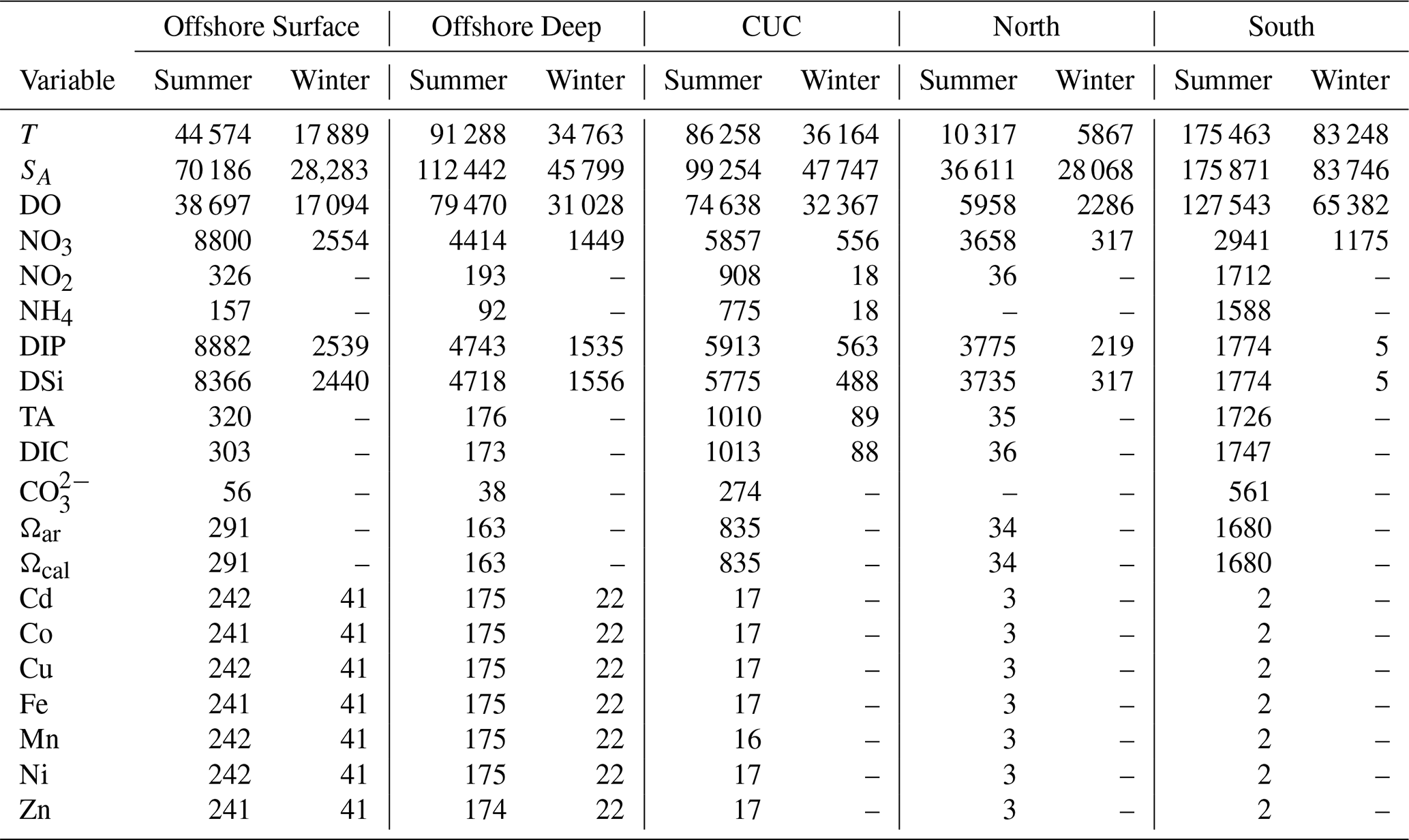
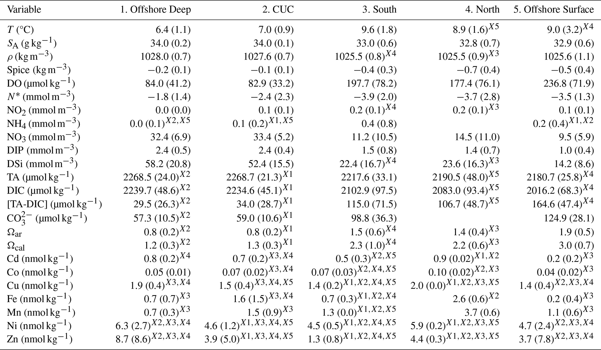
Table A3 Mean (standard deviation) of observed source water properties. Superscripts of the letter “X” followed by a number denote the source waters with which a given property is not significantly different at the 0.05 confidence interval, the number corresponding to each source water is provided in the table header.