Variability of greenhouse gas (CH₄ and CO₂) emissions in a subtropical hydroelectric reservoir: Nam Theun 2 (Lao PDR)

Hydroelectric reservoirs, though fundamental to renewable energy generation, are increasingly recognized as important sources of greenhouse gases (GHGs) in tropical and subtropical regions. However, substantial uncertainty persists regarding their contributions to the GHG cycle and their overall climate impact. Here, we present a 14 year dataset (2009–2022) of CH₄ and CO₂ emissions from the Nam Theun 2 reservoir in Lao PDR. We report emissions through diffusion, ebullition, and downstream degassing below turbines and spillways. This work represents one of the longest continuous records of reservoir GHG emissions in a subtropical system. Complementary eddy covariance approach was also employed, the results showed that CO₂ emissions were consistently higher than those estimated from discrete sampling, likely due its ability to capture real-time turbulence and hot moments, and to the location of the EC system in shallow, high-emission areas for the last two campaigns. In contrast, CH₄ emissions upscaled from EC measurements were often lower than those derived from discrete sampling, particularly during later campaigns. This difference was attributed to spatial coverage limitations, meteorological influences, wind filtering, and the lower sensitivity of the EC system to episodic ebullition events. CH₄ showed a clear diurnal pattern; while CO₂ fluxes differed between day and night only during periods of strong stratification. In this study, discrete sampling provided broader spatial coverage and higher data availability; therefore, it was used for emission calculations. CH₄ emissions peaked during the warm dry period due to lower water levels and intensified stratification that favored methanogenesis and ebullition, whereas CO₂ emissions peaked during cold dry season overturn events that released accumulated hypolimnetic carbon. Across the study period, ebullition accounted for 77 % of total CH₄ emissions and remained relatively stable, supported by substantial flooded organic matter reserves. In contrast, during that same period, diffusive CH₄ fluxes declined by 97 %, and CO₂ emissions – dominated by diffusive fluxes (96 %) – declined by 87 %, indicating reservoir aging and pro gressive depletion of labile organic matter. Over 14 years, cumulative gross emissions totaled 10 736 Gg CO₂ eq., with CH₄ (51 %) slightly exceeding CO₂ (49 %). Annual emissions were greatest in 2010 (1276 Gg CO₂ eq.), declining by ∼70 % by 2021. These findings provide new insight into long-term GHG budgets in subtropical reservoirs, refine global carbon budget estimates, and inform climate-sensitive hydropower planning.

1 Introduction

Hydroelectric reservoirs are central to global renewable-energy systems, and their number continues to expand rapidly, particularly in tropical and subtropical regions. As of December 2024, the The International Commission On Large Dams (General Synthesis, 2025) reports 62 339 registered large dams worldwide, of which approximately 17 % (10 567 dams) are operated for electricity generation. Although hydropower is widely regarded as a clean and low-carbon energy source, increasing evidence indicates that reservoirs can act as substantial sources of greenhouse gases (GHGs), raising uncertainty about their net climate benefits (Barros et al., 2011; Bastviken and Johnson, 2025; Deemer et al., 2016; Prairie et al., 2018; St. Louis et al., 2000; Yan et al., 2021).

Reservoir GHG emissions – primarily methane (CH₄) and carbon dioxide (CO₂) – originate from microbial degradation of flooded organic matter (OM) and watershed inputs. Global estimates vary widely, highlighting the magnitude of uncertainty: St. Louis et al. (2000) reported the highest values (1833 $\mathrm{Tg}{\mathrm{CO}}_{\mathrm{2}}\mathrm{eq}.{\mathrm{yr}}^{-\mathrm{1}}$ for CH₄ and 990 $\mathrm{Tg}{\mathrm{CO}}_{\mathrm{2}}\mathrm{eq}.{\mathrm{yr}}^{-\mathrm{1}}$ for CO2), while Barros et al. (2011) estimated 100 and 176 $\mathrm{Tg}{\mathrm{CO}}_{\mathrm{2}}\mathrm{eq}.{\mathrm{yr}}^{-\mathrm{1}}$, and Hertwich (2013) suggested 243 and 278 $\mathrm{Tg}{\mathrm{CO}}_{\mathrm{2}}\mathrm{eq}.{\mathrm{yr}}^{-\mathrm{1}}$, respectively. Emissions are generally highest in warm tropical systems, where elevated temperatures and OM loading enhance methanogenesis and mineralization (Barros et al., 2011).

CH₄ production occurs predominantly under oxygen-depleted conditions during the mineralization of flooded organic matter from soil and vegetation. According to Deemer et al. (2016), CH₄ emissions constitute approximately 80 % of total CO₂ eq. emissions from reservoir water surfaces, a percentage which could reach up to 90 % when calculated over a span of 100 years. The primary emission pathways include ebullition – the release of methane rich bubbles from sediments, diffusive fluxes – the transfer of dissolved gases from surface water to the atmosphere driven by concentration gradients, and degassing – the outgassing downstream of turbines, dams, or spillways caused by pressure reduction and turbulence. Ebullition can be the dominant mechanism and contributes about 65 % of total CH₄ emissions, while diffusion can account for the remaining 35 % (Deemer et al., 2016). However, neglecting degassing can lead in some cases to an underestimation of CH₄ emissions, as degassing can be a major emission pathway that can account for up to 70 % of total CH₄ emissions in some tropical reservoirs (Abril et al., 2005; Harrison et al., 2021, p. 2020; Soued and Prairie, 2020).

CO₂ emissions from reservoirs arise primarily from the supersaturation of CO₂ at the water surface. This supersaturation results from heterotrophic respiration driven by terrestrial carbon inputs from the watershed and flooded OM (Abril et al., 2005). CO₂ from reservoirs is predominantly emitted to the atmosphere through diffusive fluxes and degassing (Deshmukh et al., 2018). Emissions of CO₂ can vary significantly at daily (day-night) (Liu et al., 2016; Podgrajsek et al., 2015) and seasonally (Morales-Pineda et al., 2014) scales, and episodically, in response to weather-induced hot moments (Liu et al., 2016).

GHG fluxes from reservoirs exhibit considerable temporal as well as spatial variability (Colas et al., 2020; Guérin et al., 2016). This variability is influenced by multiple factors, including fluctuations in changes in water column depth linked with changes in precipitations and water discharge, variations in carbon and nutrient inputs from the watershed, and seasonal shifts in temperature (Abril et al., 2005; Linkhorst et al., 2020). Therefore, acquiring representative measurements at high spatial and temporal resolution is crucial for accurately estimating emissions at the reservoir scale.

At the Nam Theun 2 (NT2) reservoir in Lao PDR, 14 years of monitoring have been conducted using discrete dissolved-gas sampling and pathway-specific flux measurements (Deshmukh et al., 2014, 2018; Guérin et al., 2016; Serça et al., 2016). Complementary eddy covariance (EC) field campaigns provided footprint-integrated observations that capture diurnal variability and episodic flux events (Deshmukh et al., 2014; Erkkilä et al., 2018). This study analyzes seasonal and long-term (2009–2022) trends in CH₄ and CO₂ emissions from NT2, quantifying diffusive, ebullitive, and degassing contributions and identifying key environmental drivers. By integrating multi-emission pathways, we refine reservoir-scale carbon budgets and improve understanding of hydropower system climate impacts in subtropical regions.

2 Materials and methods

2.1 Study site

The Nam Theun 2 Reservoir (Fig. 1), located atop the Nakai Plateau in the Khammouane Province of Lao PDR, was impounded in April 2008. It attained its first maximum water level of 538 m above sea level ($\mathrm{m}\mathrm{a}.\mathrm{s}.\mathrm{l}.$) in October 2009, and was commissioned in April 2010. Detailed descriptions on the main characteristics of this trans-basin hydroelectrical project are provided in Descloux et al. (2016). The construction of the reservoir resulted in the flooding 5.12±0.68 Mt C of various types of land-cover, notably forests, agriculture lands and wetlands (Descloux et al., 2011).

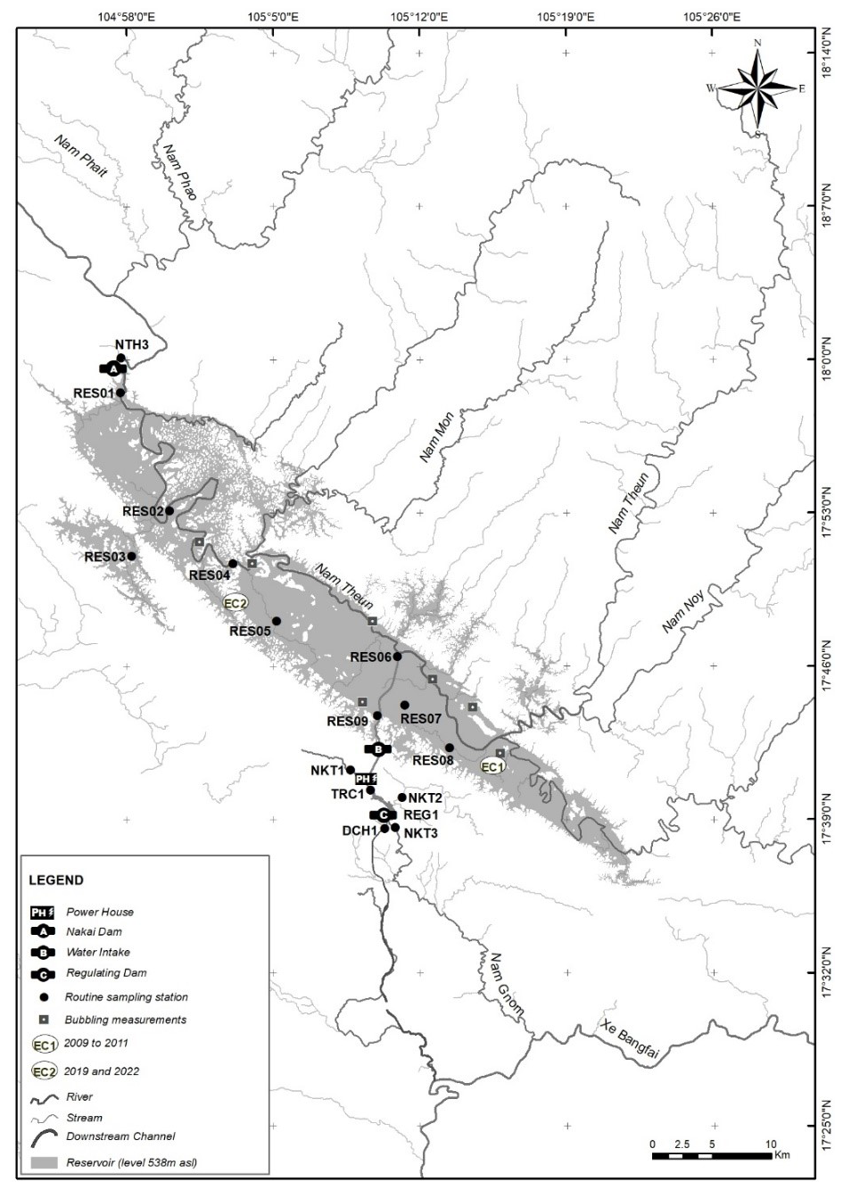
Figure 1 Map of the Nam Theun 2 Reservoir (Lao People's Democratic Republic) with routine monitoring stations and occasional EC stations; see detail on stations in Sect. 2.2.

Situated within the sub-tropical climate zone of Northern Hemisphere (17°59^′49^′′ N, 104°57^′08^′′ E) and influenced by monsoons, the reservoir experiences three distinct seasons of equal duration, namely the cold dry season (CD, from mid-October–mid-February), the warm dry season (WD, from mid-February–mid-June), and the warm wet season (WW, from mid-June–mid-October). Regardless of the season, daytime is considered to start at 06:30 and end at 18:30 daily (GMT+7).

Over the study period from 2009–2022, the seasonally averaged air temperature was lowest during the CD season (19.6±3.3 °C), whereas the warm seasons exhibited relatively stable temperatures, with 23.9±2.9 °C in WD and 23.6±1.3 °C in WW (Fig. 2A). The wind speed at the reservoir by ERA5 reanalysis (Muñoz-Sabater, 2019) was relatively low, with values ranging from 0.34–5.19 m s⁻¹. The WD exhibited an average wind speed of 1.4±0.6 m s⁻¹, while the WW had average wind speed of 1.3±0.6 m s⁻¹. In contrast, the CD experienced a relatively higher average wind speed of 2.0±0.8 m s⁻¹ (Fig. 2B). The annual average rainfall (2009–2022) recorded at the site was 2445 mm, with approximately 80 % of the rain events occurred in the WW season (Deshmukh et al., 2014; Guérin et al., 2016). The years with the highest rainfall were 2011 (3162 mm) and 2018 (3302 mm), while the driest years were 2020 (1706 mm) and 2022 (1802 mm) (Fig. 2E).

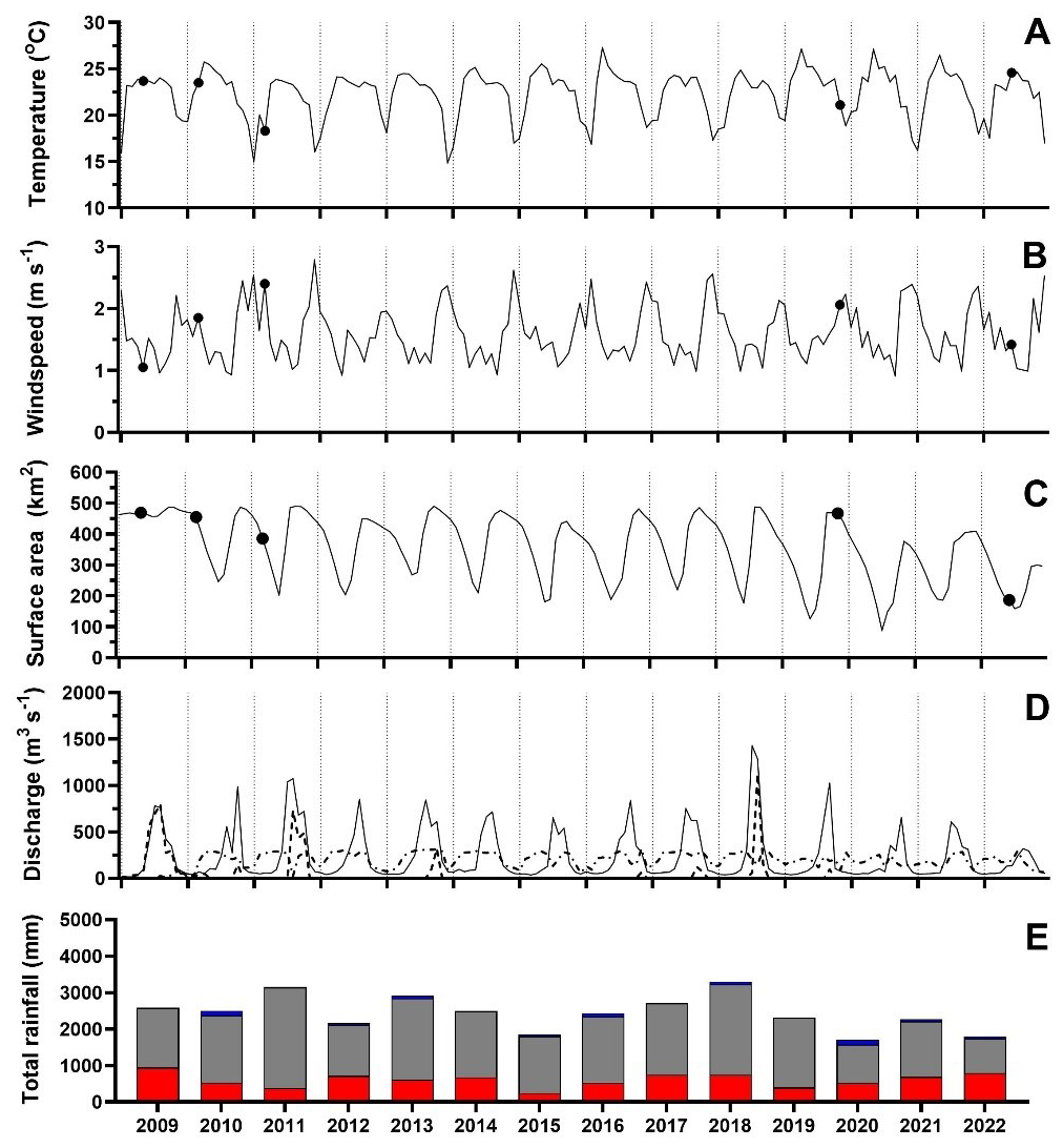
Figure 2 Monthly averages of air temperature (A), windspeed (B), reservoir surface area (C), discharge (D), and annual total rainfall (E). In the first 3 graphs, black dots represent the given parameters during the eddy covariance campaigns. In graph (D), solid line represents input discharge, dot-dash line represents output to the powerhouse and dot line represents the spillway the release at the Nakai Dam (see symbol A in Fig. 1). In graph (E), respective total rainfall is given in red, grey and blue for the WD, WW, and blue seasons.

Due to the significant variations in rainfall, the water level can change drastically between the lowest water level in the WD season and the highest one in the CD. During the course of the study, water level changed between a lowest 525.31 $\mathrm{m}\mathrm{a}.\mathrm{s}.\mathrm{l}.$ (2020) and a highest 538.36 $\mathrm{m}\mathrm{a}.\mathrm{s}.\mathrm{l}.$ (2019). As a matter of consequences, the reservoir surface area ranged between 81.9 and 499.1 km², with similar seasonal pattern to the water level variation (Fig. 2C). Categorized as shallow, the reservoir had an average depth of 7.8 m (Deshmukh et al., 2014).

Over the 14 years of measurements (2009–2022), the reservoir received an average input discharge of 238.2 m³ s⁻¹ from upstream almost pristine rivers, with large seasonal variations. During the warm wet (WW) season, the average input was 533.2 m³ s⁻¹. This inflow decreased progressively from CD season, where it stood at 100.5 m³ s⁻¹, to the WD season, where it decreased down to 79.8 m³ s⁻¹. The water was permanently discharged to the downstream of the reservoir through the dam and to the powerhouse – and occasionally from the spillway. The spillway release was occasionally used from October 2009–April 2010, i.e. before the complete operation of the hydropower plant. Since then, it has been only used to flush the occasional flood from the reservoir during raining seasons (Fig. 2D). The release at the Nakai Dam to the Nam Theun River was approximately 2.0 m³ s⁻¹ on daily average, and remained more or less constant (instream flow). Discharge to the powerhouse (Fig. 1, symbol PH) or output discharge started with commissioning in April 2010, and was on average equal to 208.4 m³ s⁻¹ (Fig. 2D).

2.2 Sample strategies

Nine monitoring stations (RES1–RES9) across the reservoir area, one station downstream of the turbine, at the inlet of the artificial downstream channel (DCH1), and three station on Nam Kathang rivers (NKT1, 2, 3) were set up to collect water temperature, dissolved oxygen concentration, dissolved concentration of CH₄, and carbon species (total inorganic carbon IC, dissolved organic carbon DOC, and particulate organic carbon POC) in the water column (see details in Sect. 2.3). Details on the characteristics of each station can be found in Descloux et al. (2016) and Guérin et al. (2016). Notably RES1 was 100 m upstream of the Nakai Dam and RES9 was located 1 km upstream of the water intake (Fig. 1, symbol B). In the reservoir, between three and six water samples were collected along the vertical profile, from the surface to the bottom, depending on the presence of stratification features such as the thermocline and oxycline. In-situ parameters such as temperature and dissolved oxygen concentration were recorded at different intervals throughout the water column (see Sect. 2.3). By contrast, at river and downstream channel stations, only surface water samples were obtained (Chanudet et al., 2016).

From January 2009–April 2017, the sampling was conducted weekly or fortnightly. After this period, the monitoring network was optimized by focusing on key stations, and sampling continued on a monthly basis.

CH₄ ebullition was collected using the submerged funnel technique (Deshmukh et al., 2014) during three periods: from May 2009–June 2011 through five different field campaigns, from March 2012–September 2013, with a weekly sampling frequency, and from March 2014–September 2022, with a monthly sampling frequency. During the first two periods, samples were gathered at seven stations, covering various types of flooded land-cover, namely dense, medium, light and degraded forests, as well as agricultural soils and all water depth. From 2014 the number of stations was reduced to three, covering dense and degraded forests along with agricultural soil and the depth of sampling sites limited to 0.4–16 m since no ebullition occur deeper in this reservoir (Deshmukh et al., 2014).

The EC system was deployed in five field campaigns: a 7 d deployment in May 2009, at the transition from the WD to the WW season; a 14 d campaign in March 2010; and a 5 d campaign in March 2011 at the transition between the CD and the WD season (Deshmukh et al., 2014). A 24 d measurement campaign was conducted in November and December 2019, during the CD season, and a 12 d campaign in June 2022, at the transition between the WD and the WW season. The first three EC campaigns were located near the RES8 station (17°41.56^′0^′′ N, 105°15.36^′0^′′ E), with a tower installed in the middle of the reservoir surface. As a matter of consequence, the EC footprint area was homogeneous in all wind direction with the same water column depth. The latter two deployments occurred near the RES4 station (17°48^′26.8^′′ N, 105°03^′27.9^′′ E). The tower was then located on the shore of the reservoir, approximately 1 m from the shoreline (fluxes were removed when they were coming from non-water surface).

Air temperature, wind speed and direction data were obtained from the ERA5-Land reanalysis dataset (Muñoz-Sabater, 2019), with data provided at hourly intervals. Daily rainfall data were recorded by rain gauges located at Nakai dam (close to RES1).

Daily water level measurements were conducted at Thalang station (RES4). Using the water level data in conjunction with the reservoir capacity curve (NTPC, 2005), daily area and volume calculations of the reservoir were performed. Precise daily outflow measurements from the reservoir were taken at two points: Nakai Dam (RES1) and the Powerhouse (RES9). Additionally, in the regulation pond downstream, daily outflow to the downstream channel (DCH1), inflows and outflow of the Nam Kathang River were also monitored. Total daily inflows to the reservoir, including tributaries and rainfall, were determined through a mass balance approach. This calculation considered changes in water volume and monitored outflows (Chanudet et al., 2012).

2.3 Measurement of Temperature, Dissolved Oxygen, Carbon Species, CH₄ and CO₂ concentrations

Water temperature and dissolved oxygen concentration were measured in situ using a Quanta^® multi-parameter probe (Hydrolab, Austin, Texas) with vertical resolution intervals of 0.5 m for the upper 5 m, and 1 m below, extending to the bottom of the sampling site.

Additionally, for laboratory analysis, water samples were continuously collected since January 2009. Surface samples were acquired using a surface water sampler (Abril et al., 2007), while samples from various depths in the water column were collected using a Uwitec water sampler. Depending on the station depth, three to six samples were collected from the surface to the oxic-anoxic interface and down to the bottom of the stations.

For dissolved CH₄ concentration, the headspace method (Guérin and Abril, 2007) was conducted by collecting two 60 mL glass vials (2 replicates) at each depth. To ensure the absence of bubbles in the water, a water flow with a volume at least three times that of the vial was flow through it. Subsequently, the vial was carefully capped using a butyl cap and secured with aluminium crimps. In the laboratory, approximately 30 mL of headspace was created by injecting N₂ to the vials. The vials were then treated with 0.3 mL of mercury chloride (1 mg L⁻¹). Subsequently, the vial was strongly shaken to ensure gas-liquid equilibrium. The vial, then, was allowed to stabilize at room temperature (25 °C) for at least one hour, and stored to be analysed within 15 d. CH₄ dissolved concentrations in the headspace were determined using gas chromatography (GC) with a flame ionization detector (FID) (SRI 8610C gas chromatograph, Torrance, CA, USA). Each injection into the GC necessitated 0.5 mL of gas collected from the headspace. Calibration was conducted using commercial CH₄ gas standards of 2, 10, and 100 ppmv, in a mixture with Nitrogen (N₂). Duplicate injections of samples exhibited a reproducibility rate higher than 5 % (Deshmukh et al., 2018; Guérin et al., 2016). Finally, to determine the dissolved concentration, the CH₄ gas solubility, as a function of temperature and salinity, as described by Yamamoto et al. (1976), was used. A salinity value of 0 was assumed in all samples.

For carbon species, filtered (0.45 µm, Nylon) and unfiltered samples were collected and analysed using an IR spectrophotometry for DOC, and with an automated Shimadzu TOC-VCSH analyser for IC and total organic carbon (TOC). POC was then determined by subtracting the DOC concentrations from the TOC measurements (Chanudet et al., 2016; Deshmukh et al., 2018).

The dissolved CO₂ concentrations were computed using the CO2sys model (Lewis and Wallace, 1998), which relied on the carbonic acid dissociation constants found in Millero (1979) for freshwater, along with the CO₂ solubility constants from Weiss (1974). IC and pH using the NBS scale, together with water temperature and salinity, were employed to estimate the dissolved CO₂ concentration from every water sample collected. the salinity value of 0 was assumed.

2.4 Diffusive flux calculation

The CH₄ and CO₂ diffusive fluxes were computed based on the surface dissolved gas concentrations and the thin boundary layer (TBL) equation. These fluxes were determined by the gradient of gas concentrations at the water–air interface with:

$$\begin{array}{}\text{(1)}& F=k_T\times \mathrm{\Delta }C\end{array}$$

Where F represents the diffusive flux at the water–air interface, ΔC denotes the concentration gradient between the water and the air and k_T stands for the gas transfer velocity at temperature (T) with:

$$\begin{array}{}\text{(2)}& k_T=k_{\mathrm{600}}\times (\mathrm{600}/{\mathit{\text{Sc}}}_T{)}^n\end{array}$$

in which Sc_T represents the Schmidt number of the gas at temperature (T) (Raymond et al., 2012). The exponent n was determined based on the wind intensity on the day of measurement, taking a value of either $-\mathrm{2}/\mathrm{3}$ for wind speeds below 3.7 m s⁻¹, and $-\mathrm{1}/\mathrm{2}$ for higher wind speeds (Jähne et al., 1987).

For k₆₀₀ within the reservoir, we combined the two k₆₀₀ equations from Guérin et al. (2007) and MacIntyre et al. (2010) in order to consider both the effect of windspeed (m s⁻¹) and rainfall (mm h⁻¹) (Deshmukh et al., 2014; Guérin et al., 2016). At station RES9, located upstream of the water intake, a constant value of 10 cm h⁻¹ was assigned to k₆₀₀. This decision was based on the particular turbulence (eddies, water current) observed in this area (Guérin et al., 2016) due to the strong water withdrawing.

To compute the total diffusive flux from the reservoir, the total area was attributed to the nine stations. Regarding the physical model presented in Chanudet et al. (2012), RES9 was handled separately due to its unique hydrological and hydrodynamic attributes. A fixed area of 3 km², consistent throughout the study period, was allocated to RES9. Similarly, RES3 located in the middle of the flooded forest, representing an separate area of the reservoir, constituting 5.5 % of the total area when at full water level, was treated independently, unaffected by temporal variations (Chanudet et al., 2012).

A series of statistical tests were conducted using GraphPad Prism (GraphPad Software, Inc.) to ascertain the possibility of grouping the remaining seven stations for the area after excluding RES3 and RES9. Initially, a normality test was conducted to assess whether the data followed a normal non-normal distribution. Subsequently, Kruskal–Wallis and Mann–Whitney tests were employed to explore similarity. The analysis confirmed that there were no significant differences between the fluxes observed at the seven stations regarding spatial variation. Consequently, the fluxes at the stations RES1, RES2, RES4, RES5, RES6, RES7, RES8 were averaged all together for the calculation of the total diffusive emission.

2.5 Degassing calculation

The degassing is assessed by the difference of concentrations of dissolved gases (C) upstream and downstream of the degassing structure. This difference was then multiplied by the corresponding discharge (Galy-Lacaux et al., 1997) with:

$$\begin{array}{}\text{(3)}& \text{Degassing}=(C_{\text{upstream}}-C_{\text{downstream}})\times \text{discharge rate}\end{array}$$

The first degassing site is located downstream of the Nakai Dam. Notably, in the dam's design, the release gate was positioned within the epilimnion of the water column. Consequently, for the upstream component, concentrations from the surface to a depth of 10 m at RES1 were averaged. The surface concentration at NTH3 (Nam Theun River) was considered for the downstream component.

The second degassing site is located downstream of the powerhouse, specifically in the upper section of the downstream channel. At this site, the balance accounted for inputs from RES9 and the Nam Kathang River (sampling points NKT1 and NKT2), and outputs discharging into the downstream Nam Kathang River (NKT3) and the downstream channel (DCH1). Since the water is permanently mixed over the whole profile at RES9, the average concentration from surface to bottom was used there, while surface concentrations were used for the other stations.

2.6 Gap-filling method

Due to technical difficulties such as GC failure, as well as unexpected circumstances during the Covid-19 pandemic and closure of the turbines for maintenance, some data gaps were observed with no sampling for an entire month for some particular station. To address this issue, a gap-filling method was applied based on seasonal averaging. Each season (based on the three distinct seasons – WD, WW, CD – in a year previously mentioned) comprising four months. In cases where one, two, or three months of data were missing within a season, the available data from the remaining month(s) of that same season were used to compute a seasonal average. This average was then used to fill the missing values for the corresponding month(s), ensuring consistency and minimizing bias in the seasonal estimates.

2.7 Ebullition calculation

In this study, an artificial neural network (ANN) was used to find the best non-linear regression between ebullition fluxes and relevant environmental variables performed (similar to Deshmukh et al., 2014). We applied ANN using the “nnet” package (https://cran.r-project.org/web/packages/nnet/index.html, last access: 28 January 2025) to model bubbling fluxes. Water depth, change in water level, atmospheric pressure, change in atmospheric pressure, total static pressure, change in total static pressure, and reservoir bottom temperature data were used as explanatory variables. The database of raw data was composed of 6158 individuals ebullitive fluxes resulted from 14 years of measurements (2009–2022), leading to a final input data for ANN composed of 6158 lines and 8 columns (1 output and 7 inputs). The data set is separated into two pools, the training one (80 % out of total input data) and the validation one (20 % out of total input data). The repeated cross-validation with 10 folds and 5 repetitions were applied to evaluate the performance of the ANN model. Additionally, the ANN model was iterated for 20 times. Averages of the 20 modelled values were used to estimate daily bubbling fluxes and the standard deviation was used to quantify the uncertainty in the estimates, the overall model performance reached up to 66 % on the daily time scale.

2.8 Gross emission calculation in CO₂ equivalents (CO₂ eq.)

In this study, we were interested in the diffusive, ebullition, and degassing emissions of CH₄ and CO₂ following reservoir impoundment, and quantity defined as the gross emission. Emission pathways from the drawdown area and diffusive fluxes downstream are excluded from the scope of this work. CH₄ emission components were converted to CO₂ eq. using a factor of 27 which represents, as defined by the IPCC (2021), the global warming potential (GWP) of non-fossil methane relative to CO₂ over a 100 year period. Subsequently, the flux from the different pathways were summed to determine the total emissions for each gas, as well as the overall gross emissions of the reservoir, categorized by seasons and years.

2.9 EC system setting and data processing

The calculation of CH₄ and CO₂ EC fluxes involved assessing the covariance between scalar variables and vertical wind speed fluctuations, complying to the well-established protocols (Aubinet et al., 2001). Fluxes were positive when indicating fluxes from the water surface to the atmosphere, and negative when from the reverse direction (Deshmukh et al., 2014).

The EC set-up comprised a 3D sonic anemometer, specifically the Windmaster Pro (Gill Instruments, Lymington Hampshire, UK) used during the first two field campaigns in May 2009 and March 2010, and a CSAT-3 (Campbell Scientific, Logan, UT, USA) employed during the last three campaigns (in 2011, 2019 and 2022). Additionally, for all the campaigns, an open-path ${\mathrm{CO}}_{\mathrm{2}}/{\mathrm{H}}_{\mathrm{2}}\mathrm{O}$ infrared gas analyser (LI-7500, LI-COR Biosciences, Lincoln, NE, USA) and a closed-path fast CH₄ analyser (DLT100, FMA from Los Gatos Research, CA, USA), were used. Air was carried to the DLT-100 through a 6 m-long tube (Synflex-1300 tubing; Eaton Performance Plastics, Cleveland), featuring an internal diameter of 8 mm. Positioned 0.20 m behind the sonic anemometer, the tube inlet was shielded with a plastic funnel to prevent ingress of rainwater. Furthermore, an internal 2 µm Swagelok filter was used to safeguard the sampling cell against dust, aerosols, insects, and droplets. High-frequency air sampling was achieved through the use of a dry vacuum scroll pump (XDS35i, BOC Edwards, Crawley, UK), delivering a flow rate of 26 L min⁻¹. Data acquisition was facilitated by a Campbell datalogger (CR3000 Micrologger^®, Campbell Scientific). Given the remote location of our study site during the first three campaigns, a 5 kVA generator running on gasoline provided power for the entire EC instrumentation setup. From 2019, the power was provided directly from a domestic facility close to the site. To ensure the atmospheric CH₄ and CO₂ concentration measurements were coming from solely the water body, tests were conducted using wind direction and a footprint model (Kljun et al., 2004).

During each EC deployment, parameters such as wind speed, atmospheric pressure, air temperature, relative humidity, and rainfall were measured using a WXT 510 device (Vaisala, Finland). In addition, incoming and outgoing shortwave and longwave radiations were measured by a radiometer (CNR-1, Kipp & Zonen, Delft, the Netherlands).

The CH₄ and CO₂ EC fluxes were calculated from the 10 Hz raw data file using EdiRe software (Clement, 1999) for the first three campaigns from 2009–2011 (see detailed setting in Deshmukh et al., 2014) and EddyPro software for the last 2 campaigns (version 7.07, LI-COR). The timestep used in both cases was 30 min average.

For the EddyPro setup, while generally similar to the EdiRe configuration, initially, a spike removal procedure was applied to identify and eliminate outlier data, allowing for a maximum spike occurrence of 5 % (Vickers and Mahrt, 1997). Secondly, a tilt (coordinate) correction was employed using the double rotation method. Thirdly, frequency response loss corrections were implemented to address flux losses at both low and high frequencies, including the application of high-frequency correction factors to account for losses coming from inadequate sampling rates (Moncrieff et al., 1997). Fourthly, time lag compensation for close-path DLT-100 CH₄ analyser was enabled. Fifthly, the turbulence fluctuations were calculated using block-averaging method, which involved determining the mean value of a variable and assessing turbulence fluctuations by measuring deviations of individual data points from this mean (Gash and Culf, 1996). Lastly, the compensation of density fluctuation by Webb–Pearman–Leuning density correction (Webb et al., 1980) was used only for CO₂ flux calculation.

2.10 Quality control of EC fluxes

A comprehensive set of criteria was employed to determine the acceptance or rejection of fluxes, as described in Deshmukh et al. (2014). Fluxes were tested for non-stationarity based on the methodology proposed by Foken and Wichura (1996) where fluxes were deemed acceptable only if the difference between the mean covariance of sub-records (5 min) and that of the entire period (30 min) fell below 30 %. Then, fluxes were discarded if their intermittency surpassed 1, in accordance with the criteria established by Mahrt (1998). Thirdly, ensuring the vertical wind speed component remained within specified bounds, skewness and kurtosis were utilized, following the guidelines of Vickers and Mahrt (1997), with values constrained to the ranges of (−2, 2) and (1, 8) respectively. Furthermore, the momentum flux, $u^{\prime }{w}^{\prime }$ was mandated to exhibit negativity, signifying a downward-directed momentum flux attributed to surface friction. Moreover, fluxes were invalidated in cases where wind originated from the power generator unit (2009–2011) or coming from the land (2019, 2022), in line with the footprint model presented by Kljun et al. (2004), considering variations in footprint extension and prevalent wind directions across diverse field campaigns. Moreover, a systematic quality check by EddyPro followed the flagging policies of Foken et al. (2005) and Mauder and Foken (2006) were also applied.

The acceptance rate for CH₄ fluxes in the first three campaigns was reported at 57 % (59 % for daytime and 52 % for nighttime fluxes; Deshmukh et al., 2014). For CO₂ fluxes, the application of quality control criteria resulted in the acceptance of 39 % of the flux data (38 % for daytime an 40 % for nighttime fluxes). This proportion of validated data was similar to earlier studies documenting EC measurements conducted over lakes (Erkkilä et al., 2018; Liu et al., 2016; Mammarella et al., 2015; Morin et al., 2018; Podgrajsek et al., 2015; Shao et al., 2015).

Due to the instability of measurement conditions, including electrical disturbances encountered during the latter campaigns, the removal rates for both gases increased significantly. Therefore, the diurnal variation (day vs. night measurements) was analysed only with the first three campaigns. In the 2019 campaign, the CO₂ EC system provided 24 d of measurements, of which 34 % were retained after QC/QA. In contrast, due to technical issues with the CH₄ analyser, only one day of CH₄ EC data (12:00 on 14 November 2019–12:00 on 15 November 2019) was usable, and 48 % of that day's CH₄ fluxes were retained following QC/QA. During the 2022 campaign, both CO₂ and CH₄ fluxes demonstrated similarly low acceptance rates of 12.5 % after all quality control measures applied. However, these values are consistent with the order of magnitude reported in a recent study using EC techniques for a reservoir (Hounshell et al., 2023), which faced similar issues related to wind direction filtering, instrument maintenance, and power instability.

2.11 Upscaling EC fluxes and comparison with corresponding discrete sampling

EC fluxes after quality control, were assumed to represent the flux from the entire reservoir. Accordingly, total monthly emissions for each campaign were estimated by upscaling the fluxes using the reservoir surface area. These upscaled emissions were then compared with the respective components of the gross emission, including diffusive fluxes and ebullitive fluxes (DE), calculated for the corresponding month of each campaign.

2.12 Statistical analysis

In addition to the specific statistical tests described in Sect. 2.5, further statistical analyses were conducted for other variables, including variation of physical–chemical parameters, diurnal fluxes, and seasonal and interannual emissions. Data normality was first assessed using the Kolmogorov–Smirnov test. Depending on the data distribution, group differences were then evaluated using either parametric tests (t-test or analysis of variance, ANOVA) or non-parametric tests (Mann–Whitney or Kruskal–Wallis, which compare median values). All analyses were performed in GraphPad Prism.

Standard deviation (SD) and standard error (SE) for each data set were calculated using the following equation:

$$\begin{array}{}\text{(4)}& \text{SE}=\text{SD}\times n^{-\mathrm{1}/\mathrm{2}}\end{array}$$

3 Results

3.1 Assessment of EC data compared to conventional measurements from the reservoir's water surface

CH₄ fluxes from the first three campaigns (Deshmukh et al., 2016), determined by EC, ranged from 0.18 to 26.84 $\mathrm{mmol}{\mathrm{m}}^{-\mathrm{2}}{\mathrm{d}}^{-\mathrm{1}}$ and average between 5.80 ± 0.43–7.20 ± 2.90 $\mathrm{mmol}{\mathrm{m}}^{-\mathrm{2}}{\mathrm{d}}^{-\mathrm{1}}$. At the end of the study period, the upper end of the flux range decreased to 4.06 $\mathrm{mmol}{\mathrm{m}}^{-\mathrm{2}}{\mathrm{d}}^{-\mathrm{1}}$ in 2019 and 13.72 $\mathrm{mmol}{\mathrm{m}}^{-\mathrm{2}}{\mathrm{d}}^{-\mathrm{1}}$ in 2022 as compared to the 2009–2011 period. Consequently, the average fluxes also declined in 2019–2022 (Table 1), especially in 2019, which had a high number of low fluxes, resulting in an average of 1.09±0.13 $\mathrm{mmol}{\mathrm{m}}^{-\mathrm{2}}{\mathrm{d}}^{-\mathrm{1}}$.

Table 1 Eddy covariance CH₄ and CO₄ flux data ($\mathrm{mmol}{\mathrm{m}}^{-\mathrm{2}}{\mathrm{d}}^{-\mathrm{1}}$) for five field campaigns, n: Number of Measurements.

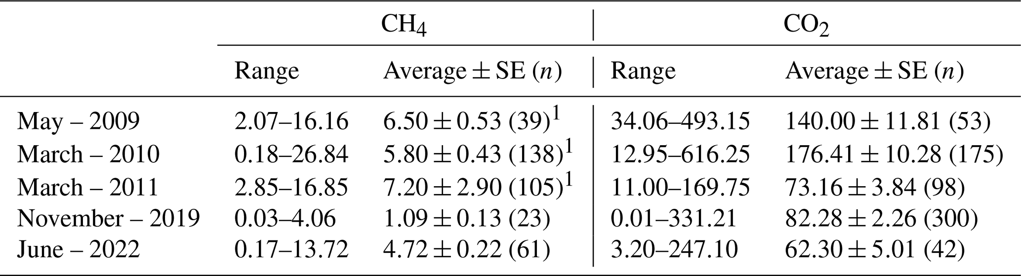
¹ Data published by Deshmukh et al. (2016).

In 2009, despite the low acceptance ratio of fluxes (Table 1), a similar trend of higher daytime emissions remained, with a 1.7-time increase in daytime fluxes over nighttime, measured at 7.57±3.02 and 4.37±2.70 $\mathrm{mmol}{\mathrm{m}}^{-\mathrm{2}}{\mathrm{d}}^{-\mathrm{1}}$ (p<0.05), respectively. 2010 showed the most significant difference between day and night CH₄ emissions, with daytime fluxes being 1.9 times higher than nighttime fluxes, measured at 6.95±5.30 and 3.63±3.70 $\mathrm{mmol}{\mathrm{m}}^{-\mathrm{2}}{\mathrm{d}}^{-\mathrm{1}}$ (p<0.05), respectively. In 2011, the daytime fluxes were 1.3 times higher than nighttime values, recorded at 8.80±3.50 and 6.30±2.10 $\mathrm{mmol}{\mathrm{m}}^{-\mathrm{2}}{\mathrm{d}}^{-\mathrm{1}}$ (p<0.05), respectively.

The reservoir acted as a source of CO₂ in the early years (2009–2011), with 30 min fluxes varying from 11.00 to 616.25 $\mathrm{mmol}{\mathrm{m}}^{-\mathrm{2}}{\mathrm{d}}^{-\mathrm{1}}$ (Table 1). On the other hand, during the last two campaigns the reservoir exhibited much lower CO₂ fluxes, reaching values as low as 0.01 $\mathrm{mmol}{\mathrm{m}}^{-\mathrm{2}}{\mathrm{d}}^{-\mathrm{1}}$ in 2019.

In 2009, the nighttime CO₂ emissions were significantly higher than daytime emissions, owing to a number of high fluxes reaching up to 493 $\mathrm{mmol}{\mathrm{m}}^{-\mathrm{2}}{\mathrm{d}}^{-\mathrm{1}}$ during the night. On average, nighttime emissions were recorded at 162±103 $\mathrm{mmol}{\mathrm{m}}^{-\mathrm{2}}{\mathrm{d}}^{-\mathrm{1}}$, surpassing the daytime average of 114±50 $\mathrm{mmol}{\mathrm{m}}^{-\mathrm{2}}{\mathrm{d}}^{-\mathrm{1}}$ (p<0.05). In contrast, the diurnal variation in CO₂ fluxes was not observed in the following years. In 2010, there was minimal difference between mean daytime and nighttime fluxes, with average values of 170±114 and 185±160 $\mathrm{mmol}{\mathrm{m}}^{-\mathrm{2}}{\mathrm{d}}^{-\mathrm{1}}$ (p=0.84), respectively. Similarly, in 2011, the variation was insignificant, with daytime fluxes averaging 77±41 and nighttime fluxes at 70±36 $\mathrm{mmol}{\mathrm{m}}^{-\mathrm{2}}{\mathrm{d}}^{-\mathrm{1}}$ (p=0.80).

For the sake of the comparison, EC fluxes were upscaled to the entire reservoir area (Fig. 3A) and calculated on a monthly basis. Two out of three campaigns in the first period indicated that CH₄ emission from EC measurements were higher than those calculated directly from the two terms: ebullition and diffusion (DE). This was the case in May 2009 (EC: 1.51±0.12 Gg CH₄ month⁻¹, DE: 0.73±0.11 Gg CH₄ month⁻¹; p<0.05) and March 2011 (EC: 1.38±0.05 Gg CH₄ month⁻¹, DE: 1.25±0.23 Gg CH₄ month⁻¹; p<0.05). This is the opposite during the March 2010 campaign with a ∼40 % higher emission from DE (1.81±0.59 Gg CH₄ month⁻¹; p<0.05) than from EC extrapolated measurement (1.31±0.10 Gg CH₄ month⁻¹; p<0.05). Similarly, DE calculated emissions were higher than the EC extrapolated ones in 2019 (EC: 0.24±0.03 Gg CH₄ month⁻¹, DE: 0.66±0.03 Gg CH₄ month⁻¹; p<0.05) and 2022 (EC: 0.42±0.02 Gg CH₄ month⁻¹, DE: 1.39±0.05 Gg CH₄ month⁻¹; p<0.05).

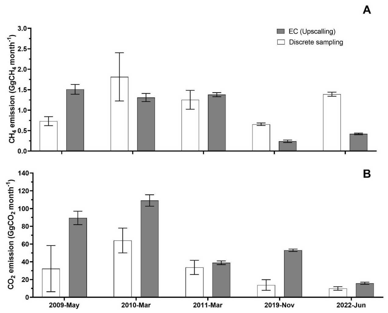
Figure 3 Comparisons of methane (A) and carbon dioxide (B) emissions (respectively in Gg CH₄ month⁻¹ and Gg CO₂ month⁻¹) by upscaling eddy covariance method (grey) and gross emissions from the reservoir's water surface without degassing (white – only diffusive fluxes and ebullition – DE) from five field campaigns in Nam Theun 2 Reservoir. The error bar represents the SE.

For CO₂ emissions, upscaled EC measurements consistently showed higher values than DE calculations (Fig. 3B). The trends between the two methods remained similar throughout the sampling periods. Specifically, in 2009 and 2019, EC (89.47±7.55 and 53.05±1.40 Gg CO₂ month⁻¹, respectively) estimates were roughly three times higher than DE calculation (32.28±26.00 and 13.85±6.00 Gg CO₂ month⁻¹, respectively) (p<0.05). In 2010 and 2022, the EC (109.12±6.37 and 15.87±1.24 Gg CO₂ month⁻¹, respectively) values were approximately twice (DE: 64.04±14.00 Gg CO₂ month⁻¹) and 1.6 times (DE: 9.96±2.00 GgCO₂ month⁻¹) higher (p<0.05), respectively. Notably, in 2011, the difference was insignificant (p=0.47), with EC measurements only being about 10 % higher than DE calculations in magnitude (Fig. 3B).

3.2 Temporal variations and vertical profiles of temperature, dissolved oxygen, greenhouse gas concentrations and carbon species in the reservoir

A set of vertical profiles from station RES4 is present in Fig. 4. RES 4 is the most comprehensively sampled site and is centrally located. That station has been used to describe long-term water-column dynamics. We extended the dataset until 2022 (Fig. 4), as earlier results (2009–2012) were previously detailed in Deshmukh et al. (2014, 2016, 2018) and Guérin et al. (2016). Over 14 years, the reservoir was thermally stratified during warm seasons (mid-February–mid-October), the strongest in the WD season with a thermocline at 4.23±1.62 m and a 7.51±3.51 °C temperature difference between surface and bottom areas. Stratification weakened in the WW season, deepening the thermocline to 5.00±2.75 m and reducing surface – bottom temperature differences to 5.57±2.76 °C. During the CD season, overturn produced a fully mixed water column with an average temperature of 21.24 ± 2.28 °C. An oxycline aligned with the thermocline, with oxygen-rich surface waters (≈6.7–6.8 mg L⁻¹) and an anoxic hypolimnion, while full mixing in CD season and sporadically in WW season oxygenated bottom waters. These seasonal patterns were consistent throughout the monitoring period.

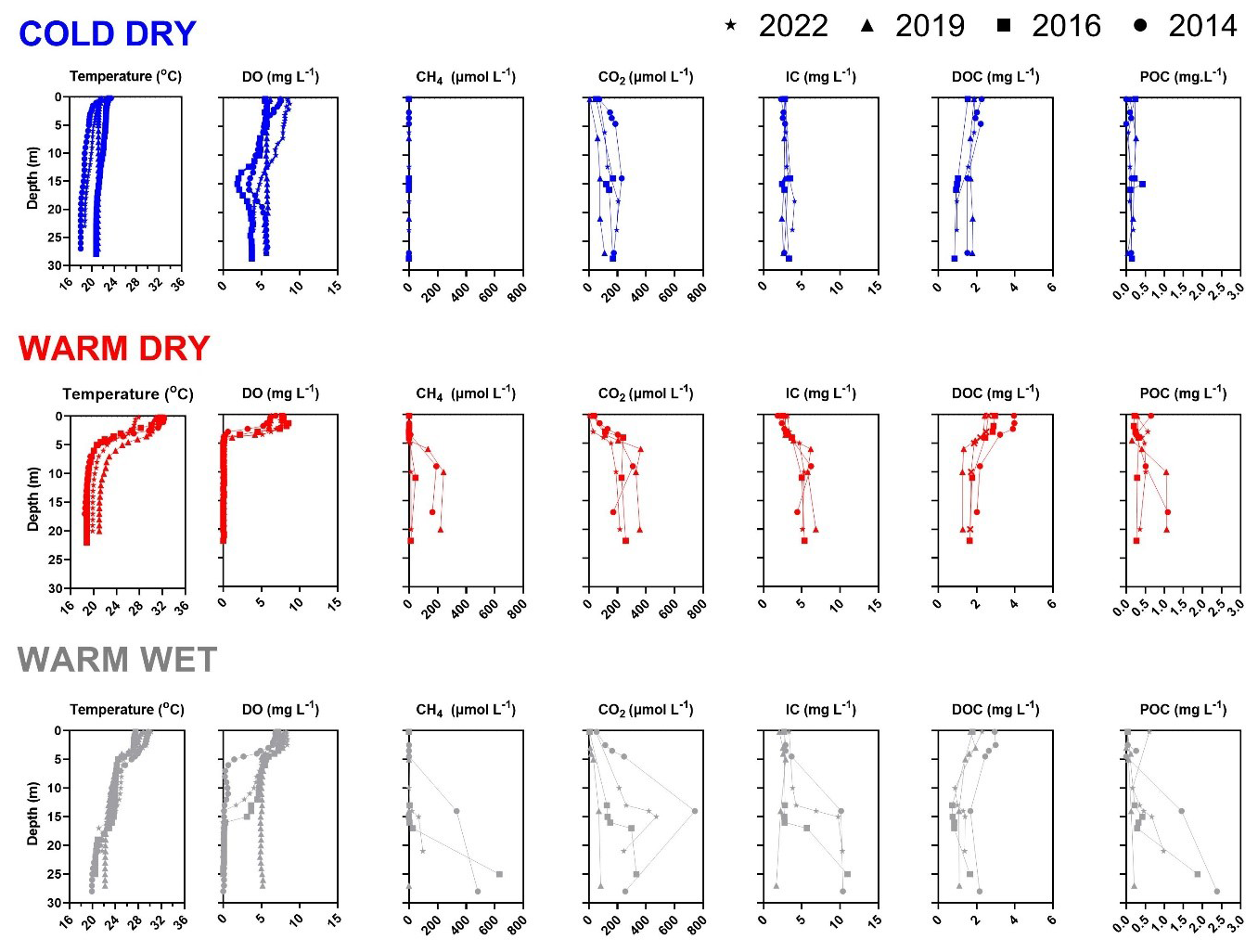
Figure 4 Vertical profiles of temperature (°C), dissolved oxygen (DO, mg L⁻¹), CH₄ (µmol L⁻¹), CO₂ (µmol L⁻¹), inorganic carbon (IC, mg L⁻¹), dissolved organic carbon (DOC, mg L⁻¹) and particulate organic carbon (POC, mg L⁻¹) at station RES4. The figure shows data from representative dates in the years 2014 (solid circle), 2016 (square), 2019 (triangle) and 2022 (star). The CD season is shown in blue, the WD season in red, and the WW season in grey.

IC ranged from 0.5–56 mg L⁻¹ and increased with depth in all seasons, with stronger gradients during WD and WW (surface: 3.5±1.3, 2.9±1.4 mg L⁻¹; bottom: 6.2±3.6, 6.8±5.6 mg L⁻¹, respectively) compared to CD (surface: 2.9±1.1 mg L⁻¹; bottom: 4.8±4.7 mg L⁻¹). Mean IC decreased seasonally from WD (4.9±2.9 mg L⁻¹) to CD (3.7±2.7 mg L⁻¹). Interannually, IC peaked in 2010 (6.2±4.7 mg L⁻¹), declined to a minimum in 2018 (2.9±1.6 mg L⁻¹), and increased to 3.9±1.5 mg L⁻¹ in 2022.

DOC ranged from 0.5–8.9 mg L⁻¹ and was consistently higher in the epilimnion (WD: 2.9±1.0 mg L⁻¹; WW: 2.4±0.9 mg L⁻¹; CD: 2.0±0.7 mg L⁻¹) than in the hypolimnion (WD: 2.1±0.7 mg L⁻¹; WW: 1.9±0.7 mg L⁻¹; CD: 1.6±0.7 mg L⁻¹). DOC followed clear seasonality ($\text{WD}>\text{WW}>\text{CD}$) and decreased from 2010 (2.5±1.0 mg L⁻¹) to 2022 (1.9±0.4 mg L⁻¹).

POC ranged from 0.01–14.3 mg L⁻¹ and was consistently lower at the surface (WD: 0.3±0.5 mg L⁻¹; WW: 0.2±0.3 mg L⁻¹; CD: 0.2±0.2 mg L⁻¹) than at the bottom (0.7±0.8, 1.1±1.2, 0.6±1.0 mg L⁻¹). Warm seasons exhibited higher POC than CD. Interannual minima occurred in 2017 (0.1 mg L⁻¹), with increases toward 2022 (0.6±1.2 mg L⁻¹).

Methane ranged from 0.002–1326 µmol L⁻¹. During warm-seasons stratification, CH₄ accumulated below the thermocline, with bottom concentrations averaging 146±184 µmol L⁻¹ in WD and 229±253 µmol L⁻¹ in WW, while surface concentrations were much lower (7.0±27.9, 3.0±16.5 µmol L⁻¹, respectively). During CD overturn, CH₄ decreased substantially throughout the water column, reaching the lowest mean (37.4±124 µmol L⁻¹). Interannually, average concentrations of CH₄ in the water column peaked pre-commissioning in 2009 (156±193 µmol L⁻¹), and reached minima in 2021–2022 (7.0±18.2, 9.3±27.4 µmol L⁻¹, respectively).

Carbon dioxide ranged from 0.1–2775 µmol L⁻¹, with mean values of 183±172 µmol L⁻¹ (WD), 212±195 µmol L⁻¹ (WW), and 168±160 µmol L⁻¹ (CD). CO₂ accumulated in bottom waters during stratification (243±198, 310±274 µmol L⁻¹) and decreased during overturn (224±238 µmol L⁻¹). CO₂ level in the water column was the highest in 2010 (305±238 µmol L⁻¹), and then it declined through 2022 (124±102 µmol L⁻¹).

3.3 Seasonal and interannual variations of CH₄ and CO₂ emissions

Over the 14 year monitoring period (Fig. 5A), the reservoir water released a total of 202.5 Gg CH₄ or around 5468 Gg CO₂ eq. The amount of CH₄ released from the reservoir water surface decreased over time after peaking at 585.4 Gg CO₂ eq. yr⁻¹ in 2010. Towards the end of the monitoring period, CH₄ emission were halved in 2021 (282.1 Gg CO₂ eq.) (Fig. 6). Most of this reduction resulted from decreases in diffusion, which dropped by 97.5 % in 2022, compared to its peak at the beginning of the study period (2009–2010) (Fig. 5A). In contrast, CH₄ ebullition did not exhibit significant variation (p=0.77, ranging from 227.6–354.9 Gg CO₂ eq. yr⁻¹, and remained the dominant pathway each year since 2010. This was especially notable after 2020, when ebullition made up more than 94 %–97.5 % of the total CH₄ emissions (Fig. 5A).

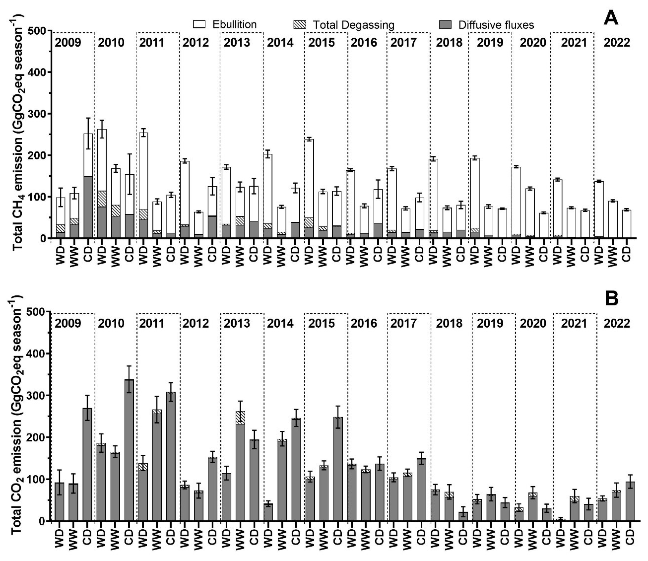
Figure 5 Seasonal variations from 2009–2022 of methane (A) and carbon dioxide (B) emissions in Gg of CO₂ equivalent by season from the three main pathways assessed: diffusive fluxes (grey), degassing (hatched) and ebullition (white). The error bar represents the total SE from all pathways combined.

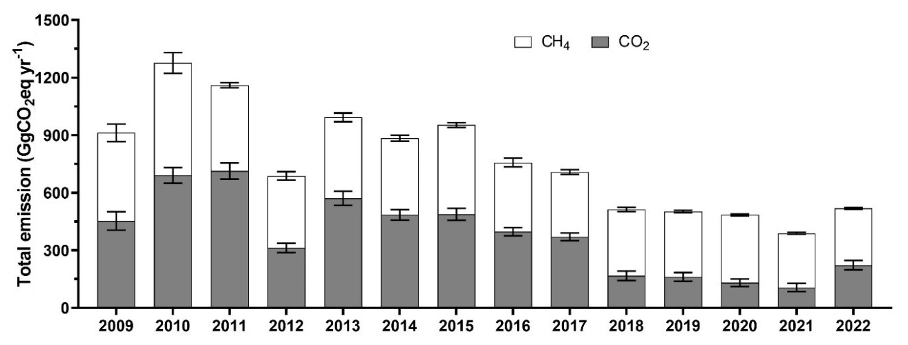
Figure 6 Annual evolution from 2009–2022 of the total greenhouse gases (CH₄ in white and CO₂ in grey emission in Gg of CO₂ equivalent by year. The error bar represents the SE of each gas.

Among the three seasons (Fig. 5A), CH₄ emissions were the highest during the WD season (for a total of approximately $\mathrm{2582}\mathrm{Gg}{\mathrm{CO}}_{\mathrm{2}}\mathrm{eq}.-\mathrm{47}\mathit{\%}$), while the WW (total approximately $\mathrm{1324}\mathrm{Gg}{\mathrm{CO}}_{\mathrm{2}}\mathrm{eq}.-\mathrm{24}\mathit{\%}$) and the CD (total approximately $\mathrm{1562}\mathrm{Gg}{\mathrm{CO}}_{\mathrm{2}}\mathrm{eq}.-\mathrm{29}\mathit{\%}$), though seasons showed no significant difference in CH₄ emissions when compared together (p=0.12). The primary pathway for CH₄ emission was ebullition, which contribute to 76.8 % of the total emissions. This pathway was most significant during the WD season, when approximately 50 % of ebullition happened, while the WW and CD seasons shared the remaining portion equally. In the course of the 14 year study, diffusion from the reservoir water surface took up 18.6 % of the total CH₄ emission. The CD season emitted the most through diffusive fluxes with 468.2 Gg CO₂ eq. (46 %), followed by WD ($\mathrm{318.8}\mathrm{Gg}{\mathrm{CO}}_{\mathrm{2}}\mathrm{eq}.-\mathrm{31}\mathit{\%}$) and WW ($\mathrm{228.0}\mathrm{Gg}{\mathrm{CO}}_{\mathrm{2}}\mathrm{eq}.-\mathrm{23}\mathit{\%}$). Degassing contributed the least to CH₄ emissions, accounting for only 4.6 % with approximately 98 % of this amount occurring during the warm seasons. From 2009–2022, CH₄ emissions via degassing and ebullition during the warm seasons did not exhibit statistically significant variation (degassing: p=0.10 for WD and p=0.11 for WW; ebullition: p=0.24 for WD and p=0.33 for WW). In contrast, diffusive fluxes during both warm seasons showed significant variation (p<0.05). During the CD season, all three emission pathways, diffusion, degassing, and ebullition, varied significantly over the study period. Total CH₄ emissions during the WW season did not change significantly over time (p=0.13), whereas significant temporal variation was observed in CH₄ emissions during the WD and CD seasons (p<0.05 for both).

Over the course of study, the total CO₂ emission (Fig. 5B) amounted to approximately 5268 Gg CO₂ eq. The decrease in CO₂ emission by 87 % from 2011 (712.9 Gg CO₂ eq. yr⁻¹) to 2021 (106.5 GgCO₂ eq. yr⁻¹) (Fig. 6) was primarily driven by diffusion at the surface of the reservoir. Degassing of CO₂ (total of 209 Gg CO₂ eq. in 14 years) did not show significant differences from 2009–2022 (p=0.232, ranging from 4.56–33.05 Gg CO₂ eq. yr⁻¹). Annually, CO₂ emissions from the reservoir gradually decreased (p<0.05), with the exceptions of 2012 and 2018, when emissions were divided suddenly by a factor two compared to the previous years. The year 2022 was also notably different with a doubling of the annual emission that year compared to the one calculated for 2021.

Among the three seasons, approximately 43 % were released during the CD season, 23 % during the WD season and the remaining 34 % during the WW season (Fig. 5B). These trends mirrored the CO₂ emission by diffusion at the air–water interface which was the dominant pathway, accounting for 96 % of the total emission of CO₂. As for CH₄, with approximately 4 % of the total CO₂ emission, degassing was a minor pathway, around 87 % being degassed during the warm seasons.

The total gross emission of both CO₂ and CH₄ together over the study period (2009–2022) were 10 736 Gg CO₂ eq., with an approximately equal distribution for both gases (CO₂: $\mathrm{5268}\mathrm{Gg}{\mathrm{CO}}_{\mathrm{2}}\mathrm{eq}.-\mathrm{49}\mathit{\%}$; CH₄: $\mathrm{5468}\mathrm{Gg}{\mathrm{CO}}_{\mathrm{2}}\mathrm{eq}.-\mathrm{51}\mathit{\%}$). Emissions were the highest in 2010, at 1276 Gg CO₂ eq. yr⁻¹, and decreased over time to the lowest point in 2021, at 389 Gg CO₂ eq. yr⁻¹ (Fig. 6). In 2009, CH₄ and CO₂ contributed equally to gross emission. From 2010–2017, CO₂ was the dominant emission source accounting for approximately 50 %–60 % of total emissions, largely due to dominant diffusive fluxes (Fig. 5B); whereas CH₄ became the primary contributor after 2018 due to constant and high ebullition rates as the main emission pathway (Fig. 5A).

Seasonal analysis showed that the highest gross emission occurred during the CD season, totalling 3841 Gg CO₂ eq., followed by the WD season with 3809 Gg CO₂ eq., and the WW season with 3086 Gg CO₂ eq. CO₂ was the dominant greenhouse gas during the WW and CD seasons, contributing 57 % and 59 % of total seasonal emissions, respectively, with diffusion at the air–water interface serving as the dominant pathway. In contrast, CH₄ was the major contributor during the WD season, making 68 % of the seasonal emission, particularly through ebullition, which remained the primary pathway throughout the entire study period. Degassing represented only 4.3 % of total CO₂ eq. emissions (considering both CO₂ and CH₄), although its contribution was more pronounced during warm periods.

4 Discussions

4.1 Methodological comparison: evaluating the differences between EC and manual discrete sampling

The position of the EC tower in the first three campaigns (Sect. 2.2) represents an ideal situation for measurement technique comparison, particularly during mixed water column conditions. However, fluxes measured with EC on one side, and traditional water measurement methods (diffusion and ebullition – DE, see Sects. 2.2–2.4 and 2.8) on the other side are representative of different spatial scales of emission sources. Furthermore, since EC fluxes are time-and-space integrated, one cannot anticipate 1:1 comparison with conventional measurements (Erkkilä et al., 2018).

According to Spank et al. (2023), inland water emissions CO₂ and CH₄ are commonly measured using methods such as manual gas sampling used to calculate fluxes with TBL, floating chambers, and bubble traps (for example, submerged funnels for this study). While these techniques deliver precise measurements, they often lack broader spatial and temporal coverage. In our case, the comprehensive sampling strategies and a set of sampling sites covering the variety of flooded ecosystems with a specific attribution of area to special sites (Sect. 2.2) accounted for the special variation. Alternatively, the EC approach enables continuous monitoring of gas fluxes across a larger footprint (up to 500 m; Deshmukh et al., 2014) and as a consequence, allows a better representativeness of the measured emissions and the exchange processes (Spank et al., 2023).

For CH₄, in the May 2009 field campaign, substantial rainfall during EC measurements (78.5 mm during the EC deployment, or 67 % of total 2009 WD precipitation, Fig. 2E), likely influenced CH₄ emissions by enhancing surface water mixing. This could have increased diffusion that EC effectively captured (1.51±0.12 Gg CH₄ month⁻¹). In contrast, DE (0.73±0.11 Gg CH₄ month⁻¹) in May 2009 is based on data with a limited spatial coverage for both water samplings and bubble traps. Therefore, calculations relied mostly on gap-filling and ANN which might have introduced bias and led to underestimations in DE. In March 2010, the reservoir was commissioned, creating a CH₄ emission hotspot at RES9 (Guérin et al., 2016), due to increased turbulence, which kept the 3 km² area upstream of RES9 constantly mixed. This mixing brought CH₄-rich bottom water to the surface and triggered high diffusive fluxes. RES9 contributed 31.7 % of total CH₄ diffusive fluxes in 2010 (Guérin et al., 2016) which is the highest proportion in the 14 year period, 100 times higher than in 2009 (when water was not sent to turbine, before commissioning). 2010 also was the year with the highest CH₄ diffusive fluxes in the course of study. As the EC was located remotely from RES9 station, the EC (1.31±0.10 Gg CH₄ month⁻¹) was unable to capture the hotspot of CH₄ diffusion (Guérin et al., 2016) and consequently, the EC estimation of the CH₄ emissions from the reservoir was necessarily lower than the DE (1.81±0.59 Gg CH₄ month⁻¹) approach. In 2011, the reduced diurnal difference in the EC fluxes (1.3 times higher during the day) might explain why EC (1.31±0.10 Gg CH₄ month⁻¹) and DE (1.25±0.23 Gg CH₄ month⁻¹) results were more comparable, as the water sampling for DE calculations occurred only during daytime (10:00–16:00). The latter two campaigns saw a relocation of the EC station. The tower was placed onshore, which limited its ability to capture both diffusive and ebullitive fluxes as these were often filtered due to unsuitable wind directions. Deemer et al. (2016) indicated that CH₄ fluxes measured as a combination of ebullition and diffusion were approximately twice as high as those from diffusion alone, consistent with the difference observed between EC and DE measurements in two campaigns (Sect. 3.3). An important consideration in interpreting the results is the role of CH₄ ebullition, which became increasingly significant during the latter half of the study period (Fig. 5). While the EC station captured fluxes continuously over time, it was limited to a single point and depth. In contrast, the discrete chamber measurements, conducted across various depths and reservoir locations, offered broader spatial coverage. Notably, because ebullition was measured over a full day cycle (24 h), its temporal resolution was comparable to that of the EC method. Therefore, the key distinction lies in spatial variability: chamber measurements captured a more representative site of ebullition across the reservoir, which was crucial for understanding the spatial heterogeneity of emissions.

CO₂ fluxes measured by the EC method consistently exceeded the DE results. This difference, also reported in previous studies (Erkkilä et al., 2018; Mammarella et al., 2015), rooted from differences in spatial resolution and sampling location between the two methods, which differently captured spatial variability in CO₂ fluxes across the lake (Scholz et al., 2021). The EC station, positioned in the middle of the open waters of the reservoir (average depth of 10–10.5 m in 2009, 2010 and 2011, Deshmukh et al., 2014) or on the reservoir shore (2019, 2022), captured fluxes from two specific water conditions. On the opposite, water samples used in TBL-based diffusive flux calculations were gathered in all kind of water depth conditions of the reservoir. Higher CO₂ emissions in shallow water as seen by EC in 2019 and 2022 is consistent with results from previous work (Loken et al., 2019; Xiao et al., 2020). Shallow areas often experience warmer water temperatures, which can stimulate microbial respiration and elevate CO₂ emissions. Additionally, in shallow zones, sediments lie closer to the water surface, and the mixing layer more readily extends to the lake bottom (Holgerson, 2015). Organic material inputs from the surrounding land, providing a rich substrate for microbial respiration and subsequent CO₂ production can be deposited close to the shoreline (Xiao et al., 2020). Thus, during the 2019 and 2022 campaigns, the position of EC towers likely contributed to the higher CO₂ fluxes observed when upscaling the results from that method. For the earlier three campaigns (2009–2011), the consistently higher EC fluxes likely result from methodological differences, including the EC method ability to capture real-time turbulent fluxes, short-term peak events (for instance, wind bursts or convective mixing), and continuous diurnal variation, in contrast to the TBL method reliance on daytime sampling and calculated gas transfer velocities. Potential underestimation of the gas transfer coefficient k_T in TBL calculations, especially under calm conditions or in the absence of direct turbulence measurements, could lead to systematically lower flux estimates. Thus, while spatial heterogeneity must explain some of the differences in later years, methodological limitations inherent to the TBL approach must have played a more central role in the earlier three campaigns. In addition, high wind events, with 70 % higher than average wind speed, captured in March 2010 (Supplement Fig. S4 in Deshmukh et al., 2014) have triggered sporadic very high CO₂ fluxes, up to 616 $\mathrm{mmol}{\mathrm{m}}^{-\mathrm{2}}{\mathrm{d}}^{-\mathrm{1}}$. Under these circumstances, CO₂-rich hypolimnetic waters were likely to be brought up to the surface water, leading to substantially larger CO₂ fluxes, as compared to calm wind period. EC continuous measurement was able to capture such events.

The results suggested the importance of integrating multiple measurement approaches to improve GHG emission estimates. By taking advantages of the continuous temporal resolution offered by EC and the broader spatial coverage achieved through discrete sampling, the overall accuracy and representativeness of emission assessments could be enhanced. Nonetheless, in this study, due to the limited number of EC campaigns and the extensive dataset available from discrete sampling, the calculation of total GHG emissions from the reservoir water relied primarily on discrete sampling data.

4.2 Diurnal variation of fluxes from EC measurement

4.2.1 CH₄ fluxes

The CH₄ diurnal variations from the first three campaigns were discussed in the study of Deshmukh et al. (2014), in which they indicated a strong relationship between hydrostatic pressure and methane emissions, particularly through ebullition, at the NT2 reservoir.

An unique bimodal diurnal variation of CH₄ emissions was attributed mainly to the changes in atmospheric pressure, which were linked to the semidiurnal pattern of atmospheric pressure influenced by global atmospheric tides (Deshmukh et al., 2014). Specifically, CH₄ emissions peaked around midnight and again near midday, following periods of atmospheric pressure drop, a phenomenon shown to trigger ebullition by reducing hydrostatic pressure at the reservoir bottom (Deshmukh et al., 2014). This effect was significant at lower water depths, where a greater relative change in total static pressure further facilitates gas release (Deshmukh et al., 2014).

Additionally, this CH₄ diurnal variation, with daytime fluxes higher than nighttime fluxes, was found by Bastviken et al. (2010) and Tan et al. (2021). The latter finding claimed that solar radiation can also play an important role in the process of aerobic methanogenesis, also known as “methane paradox” in which dissolved CH₄ concentration is supersaturated in oxic water (Tang et al., 2016). Even though the production of methane in oxygen-rich waters is not yet fully understood, recent researches indicate a strong association with algal photosynthesis, where algal growth drives CH₄ production (Bogard et al., 2014; Hartmann et al., 2020). Bižić et al. (2020) conducted experiments using light and dark conditions which suggested that cyanobacteria contribute notably to CH₄ production, directly linking this process to light-dependent primary productivity. As a matter of consequence, light availability, a major factor in photosynthetic activity (Krause and Weis, 1991), indirectly influences CH₄ production, while temperature plays a critical role in the organic decomposition associated with methanogenesis (Yvon-Durocher et al., 2014). Other studies in wetland environments have shown that primary productivity significantly modulate the daily CH₄ emission cycle with increased fluxes during the day (Hatala et al., 2012; Mitra et al., 2020). Furthermore, solar radiation appears to suppress CH₄ oxidation in the epilimnion, increasing net CH₄ emissions by limiting its breakdown in sunlit surface waters (Murase and Sugimoto, 2005; Tang et al., 2014).

Considering the diurnal variation in CH₄ fluxes, daytime fluxes (7.5 $\mathrm{mmol}{\mathrm{m}}^{-\mathrm{2}}{\mathrm{d}}^{-\mathrm{1}}$) were approximately 16 % higher than the daily mean measured by EC in 2009 (6.50 $\mathrm{mmol}{\mathrm{m}}^{-\mathrm{2}}{\mathrm{d}}^{-\mathrm{1}}$), 20 % higher in 2010 (6.95 $\mathrm{mmol}{\mathrm{m}}^{-\mathrm{2}}{\mathrm{d}}^{-\mathrm{1}}$ compared with 5.80 $\mathrm{mmol}{\mathrm{m}}^{-\mathrm{2}}{\mathrm{d}}^{-\mathrm{1}}$), and 22 % higher in 2011 (8.80 $\mathrm{mmol}{\mathrm{m}}^{-\mathrm{2}}{\mathrm{d}}^{-\mathrm{1}}$ compared with 7.20 $\mathrm{mmol}{\mathrm{m}}^{-\mathrm{2}}{\mathrm{d}}^{-\mathrm{1}}$). These differences were assumed to remain consistent throughout the study period, regardless of stratification status. The higher daytime fluxes likely reflect the diurnal difference in diffusive fluxes, as this pathway was determined from manual headspace sampling conducted exclusively during daytime, whereas bubble traps were deployed continuously for 24–48 h (Deshmukh et al., 2014). Given that diffusion contributed approximately 30 % of total emissions in 2009, 50 % in 2010, and 30 % in 2011, daytime-only sampling could result in an overestimation of total CH₄ fluxes by about 5 %–10 %.

Taken together, these findings demonstrate that diurnal CH₄ dynamics at NT2 are governed by the combined influence of physical pressure – driven ebullition and temperature- and light-dependent biogeochemical regulation of diffusive emissions. This underscores the importance of continuous high-frequency EC measurements for resolving short-term variability that cannot be fully captured by discrete daytime sampling.

4.2.2 CO₂ fluxes

High nighttime CO₂ emissions during low wind speed conditions, as seen in 2009 (Supplement Fig. S4 in Deshmukh et al., 2014), might result from waterside convection and erosion of the thermocline (Eugster et al., 2003; Jeffery et al., 2007; MacIntyre et al., 2010; Mammarella et al., 2015; Podgrajsek et al., 2015). Daytime lower fluxes could also result from the photosynthesis activity in the euphotic water column leading to a decrease of CO₂ concentrations in the upper water column.

During the daytime, absorption of solar radiation in the water column diminishes the depth of the surface mixing layer and thereby thermal convection from heat loss (Eugster et al., 2003; Podgrajsek et al., 2015). CO₂ fluxes were lower during the 2011 field campaign, even though it exhibited wind speed almost as high as in 2010 (up to 8 m s⁻¹). With low surface water temperature and with a weak thermal gradient, it seems that even high wind conditions during the daytime were not able to overcome with the heating effect on CO₂ fluxes. The diurnal variation in CO₂ emissions can also be explained by temperature-driven increases in respiration, decomposition and photooxidation of organic matter and DOC in the water column. Respiration increases CO₂ concentrations in the surface layer, leading to higher emissions, especially at night when photosynthetic CO₂ uptake from phytoplankton stops, allowing CO₂ to accumulate and be released. This balance between CO₂ consumption via photosynthesis (daytime) and CO₂ production via respiration (nighttime and daytime) (Spank et al., 2023) is in agreement with the observation in this study, especially during 2009 in which significantly higher nighttime CO₂ emissions were observed, when photosynthesis likely played a significant role in reducing daytime CO₂ fluxes.

Particularly during a strong thermal stratification period similar to May 2009 (middle of WD season), sampling only during daytime could lead to an underestimation of the daily flux (the daytime mean flux (114 $\mathrm{mmol}{\mathrm{m}}^{-\mathrm{2}}{\mathrm{d}}^{-\mathrm{1}}$) was 19 % smaller than the daily mean (140 $\mathrm{mmol}{\mathrm{m}}^{-\mathrm{2}}{\mathrm{d}}^{-\mathrm{1}}$)). Exclusion of the diurnal variability in CO₂ fluxes, for instance, not sampling nighttime fluxes, during a strong thermal stratification period could underestimate the annual mean flux by approximately 5 %. This percentage applies for the NT2 reservoir knowing that it is thermally stratified for the three months of the warm dry season (Chanudet et al., 2016; Guérin et al., 2016). Overall, CO₂ dynamics at NT2 reflect the combined effects of stratification-driven physical transport and temperature-dependent biological processes.

However, in this study, no correction was applied to account for the potential enhancement of nighttime fluxes during stratification period. As a result, while our estimates were considered robust, they should be interpreted as conservative due to the uncorrected diurnal variability for both gases.

4.3 Seasonal dynamics of GHG emissions

4.3.1 CH₄ emissions

The seasonal variations in CH₄ emissions from the NT2 reservoir illustrate the critical role of thermal stratification, water mixing, and organic matter decomposition in regulating greenhouse gas fluxes as described by Guérin et al. (2016).

During the WD season, total emissions reached their maximum due to higher temperatures and lower dissolved oxygen levels in the water column, creating more favourable conditions for methane production and reducing methane oxidation (Upadhyay et al., 2023). Stratification during this period creates distinct layers within the water column, with limited vertical mixing. This vertical isolation enhances anaerobic decomposition of organic material, thereby fuelling methanogenesis in deeper layers. Ebullitive fluxes contributed predominantly in this season, consistent with the findings of Deshmukh et al. (2014). Ebullition is well-documented to be positively correlated with temperature (Chanton et al., 1989; St. Louis et al., 2000; Zheng et al., 2022), as elevated temperatures promote CH₄ production and decrease CH₄ solubility. During the WD season, the decline in the water level reduces hydrostatic pressure on the sediment (Deshmukh et al., 2014; Maeck et al., 2014), triggering bubble release. Diffusive fluxes share similar driving parameters as ebullition, in which higher temperature and lower DO in the water column (Fig. 4) facilitate CH₄ to reach the surface as CH₄ oxidation is reduced (D'Ambrosio and Harrison, 2021). Moreover, the availability of organic matter plays a crucial role; higher carbon content in the water column (DOC and IC) during the WD season due to processes such as enhanced microbial activities, increased discharges from watershed, stronger photosynthesis, contributes to CH₄ production by supplying labile allochthonous and autochthonous OM. Degassing of CH₄ was also highest during this period, consistent with the trend reported by Deshmukh et al. (2016) after 14 years of measurements. Degassing was significant only when spillway release occurred during flooding in the later months of WD and early WW (Fig. 2D). CH₄-rich water from below the oxycline, approximately 15 m deep, was then discharged (Deshmukh et al., 2016).

In contrast, methane emissions reached their lowest levels during the WW season, characterized by a twofold decrease in ebullition and the lowest diffusive fluxes among the three studied seasons. The erosion of the thermocline during this period promoted more aerobic conditions, which favoured methanotrophic activity and thereby reduced net CH₄ emissions. Deshmukh et al. (2016) stated the reduced ebullition observed at the NT2 reservoir during the WW season to several interrelated mechanisms: (1) CH₄ concentrations within bubbles were substantially lower than those recorded during the WD season, likely due to increased oxidation of CH₄; (2) bubble CH₄ concentrations exhibited minimal variation with depth during the WW season, unlike the WD season, where elevated concentrations were confined to shallower depths, indicating the role of depth-dependent processes such as CH₄ dissolution, which can reduce CH₄ content in bubbles by up to 20 % in waters less than 10 m deep, as reported by McGinnis et al. (2006) and Ostrovsky et al. (2008); (3) lower temperatures during the WW season (Fig. 2A) led to a decrease in the methanogenic activity and increased CH₄ solubility, thereby suppressing bubble formation and release; and (4) higher water levels during WW increased hydrostatic pressure, further inhibiting ebullition. For diffusive fluxes, elevated river inflow during this season (Chanudet et al., 2012) may have produced a dilution effect, further lowering CH₄ concentrations in surface waters and reducing the efflux to the atmosphere. Increased precipitation likely also contributed to slower organic matter decomposition by diminishing the thermal gradient between surface waters and the hypolimnion. Sporadic mixing events enhanced oxygen penetration into deeper layers and flooded sediments, limiting CH₄ accumulation in the hypolimnion (Guérin et al., 2016). The weakening of the thermocline during the WW season (Fig. 4) further facilitated the downward transport of dissolved oxygen, reducing the amount of CH₄ reaching surface waters due to CH₄ oxidation. Degassing was also reduced since bottom concentrations are lower (Guérin et al., 2016), and since the water discharge at the powerhouse was reduced in order to initiate a water storage phase before WD and CD seasons (Fig. 2D).

During the CD season, vertical mixing occurred annually as surface water temperatures declined and approached those of the bottom layers (Fig. 4). Simultaneously, the reservoir surface area remained consistently high, with minimal inflow and outflow discharges (Fig. 2D). These conditions adversely affected CH₄ solubility and hindered the development of anoxic zones required for methanogenesis (Deshmukh et al., 2014). Ebullition in the NT2 reservoir is negatively correlated with both water depth and fluctuations in water level (Deshmukh et al., 2014), which accounts for the lower ebullition flux observed during the CD season compared to the WD season. The relatively stable hydrostatic pressure (Schmid et al., 2017), in conjunction with the large surface area and higher wind speeds (Fig. 2B) compared to the two warm seasons, increased the gas transfer velocity, thereby enhancing diffusive CH₄ fluxes, which peaked during this season (Guérin et al., 2007). CH₄ diffusive fluxes during this period were also significantly influenced by reservoir overturn, which occurs as thermal stratification collapses due to cooling surface temperatures. Guérin et al. (2016) previously identified reservoir overturn in NT2 as a hot moment for CH₄ emissions, where deep, CH₄-rich waters mix with surface layers, intensifying methane transport and release. The breakdown of the stratification promotes gas exchange between the hypolimnion and the atmosphere, resulting in elevated CH₄ diffusive emissions. In contrast, degassing was negligible during this season, accounting for only about 0.4 % of total seasonal emissions, due to low concentrations, minimal water discharge, and limited flood events due to low precipitation (Fig. 2E). This observation aligns with the findings of Deshmukh et al. (2016) from the early post-impoundment years.

Overall, our findings demonstrate that oxygen availability, governed by stratification – driven mixing and hydrological pressure changes, is the dominant control on seasonal CH₄ fluxes in tropical reservoirs, emphasizing the need for emission models that incorporate physical processes such as mixing – driven DO transport, water-level fluctuations, and hydrostatic pressure variation (DelSontro et al., 2018; Guérin et al., 2016).

4.3.2 CO₂ emissions

CO₂ emissions from the NT2 reservoir showed distinct seasonal patterns influenced by temperature, water column stratification, and biological activity (Deshmukh et al., 2018). The vertical profiles of CO₂ in this study found to be consistent and similar in shape with previous finding of Deshmukh et al. (2018), and with measurements from other tropical reservoirs (Abril et al., 2005; Chanudet et al., 2011; Guérin et al., 2006). Since 96 % of CO₂ emission from NT2 reservoir came from diffusive fluxes, the understanding of the variation of the dissolved CO₂ concentrations is crucial to interpret the seasonal and interannual patterns of CO₂ emissions.

In the WD season, the shape of the vertical profiles of CO₂ concentration suggest that CO₂ is mostly produced at the bottom of the reservoir, in the OM pool of flooded soil and vegetation; and consumed by phytoplankton, whose biomass is enhanced by high temperature (Fig. 2A) of the WD season (Abril et al., 2005; Barros et al., 2011; Chanudet et al., 2011; Deemer et al., 2016; Guérin et al., 2006; St. Louis et al., 2000). It is supported by the fact that the concentrations of chlorophyll a in the NT2 reservoir (unpublished data) always peaks in the WD season, promoting consumption of CO₂ in the epilimnion. Additionally, diffusive fluxes were correlated with reservoir area and wind speed as described with CH₄. Therefore, the WD season with lowest wind speed and surface area (Fig. 2B and C) led to low fluxes.

The WW season exhibited intermediate emission levels, with sporadic mixing events (Guérin et al., 2016) contributing to periodic CO₂ fluxes to the atmosphere. The erosions of the thermocline as well as the oxycline during this season (Fig. 4) allow DO to penetrate deeper into the deep water, where the pool of CO₂ production via enhanced aerobic respiration is located. The highest CH₄ oxidation rate recorded in the WW season (Guérin et al., 2016), also contributed to the gradual increase of CO₂ emissions.

During the CD season, CO₂ emissions peaked, with diffusion at the air–water interface as a major contributor. This elevated emission rate was primarily driven by overturn and complete mixing of the water column, which redistributed CO₂-rich waters from the bottom layers to the surface, facilitating their release, contributed to the “hot moment” observed for CH₄ emissions (Guérin et al., 2016). Furthermore, complete mixing and oxygenation of the water column during the CD season supported more extensive aerobic decomposition of organic matter, pelagic respiration (Bastviken et al., 2004) and the oxidation of large amount of hypolimnion CH₄ going up the vertical water column, both of which contributed to enhance CO₂ production. Hydrologically, residence time is recognized as one of the most influential factors in river damming (Prairie et al., 2018), significantly affecting the degradation rate of DOC (Dillon and Molot, 1997; Sobek et al., 2007). Carbon mineralization has been shown to positively correlate with residence time (Dillon and Molot, 1997). The CD season was consistently characterized by the longest residence times, due to minimal outflows and a larger volume (Fig. 2C and D). This coincided with the lowest DOC concentrations observed among the three seasons, suggesting enhanced carbon processing and mineralization during that period.

CO₂ degassing exhibited seasonal patterns similar to those observed for CH₄. Degassing was more pronounced during the warm seasons, driven by elevated CO₂ concentrations in the water column, high water discharges, and occasional use of the spillway. In contrast, during the CD season, when reservoir volume remains relatively stable, degassing was negligible, contributing only around 1 % of seasonal CD emissions. This seasonal pattern has remained consistent over time.

Overall, CO₂ emissions are strongly governed by stratification-driven oxygen dynamics, water column overturn, and residence time, with temperature acting primarily as a secondary amplifier. Seasonal peaks are largely associated with short-term overturn and destratification events, emphasizing the need to account for physical dynamics, oxygen distribution, and hydrological variability in monitoring and predictive models of tropical reservoir greenhouse gas fluxes. Thee reduced measurement frequency implemented after 2017 likely resulted in an underestimation of short-term CO₂ emission peaks due to overturn during the CD, and sporadic destratification during the WW (Fig. 5B). Consequently, it could lower the estimates of total emissions.

4.4 Interannual dynamics of GHG emissions

4.4.1 CH₄ emissions

From 2009–2022, CH₄ emissions exhibited a gradual decline, with peak emissions recorded after commission (2010) dropping to nearly half by the end of the study (2022). Such trends underscore the influence of reservoir age on CH₄ emissions (Barros et al., 2011), as older reservoirs tend to emit less CH₄ due to the depletion of readily degradable organic matter, with no major input beyond the initial allochthonous supply and limited autochthonous production.

CH₄ diffusion, the second most significant CH₄ emission (in CO₂ eq.) pathway from the water surface (Serça et al., 2016), has declined steadily over time, likely due to gradual changes in reservoir dynamics, such as the diminishing availability of labile OM, a better oxygenation by higher concentration of DO and enhanced methane oxidation. The hypothesis of increasing CH₄ oxidation rate in later studied years could explain part of the increase of CO₂ concentrations in 2022, despite CH₄ concentrations in the water column continued to decrease. Given that the reservoir mixing regime remained relatively constant throughout the 14 year period, the observed reduction in diffusive emissions is likely driven by biological and chemical factors rather than shifts in physical mixing. This is supported by a documented decrease in both DOC and IC concentrations in the water column over the study period, indicating lower substrate availability for methanogenesis (Colas et al., 2020). A gradual reduction in CH₄ production in deep waters would result in a diminished supply of dissolved CH₄ available for diffusion. Over a 14 year period, ebullition was the dominant pathway for CH₄ emission. This contribution is consistent with values reported for inland waters, where ebullition represents approximately 62 %–84 % of CH₄ emissions (Zheng et al., 2022), and for shallow lakes and ponds, where the contribution ranges from 50 %–90 % (Attermeyer et al., 2016; Saunois et al., 2020). It also surpasses the average estimated contribution of 65 % from reservoirs globally (Deemer et al., 2016). The persistence of ebullition as the primary emission pathway can be attributed to its dependence on the decomposition of the flooded organic matter and bubble formation. Although ebullition was anticipated to decline over time as the labile parts of flooded OM decreased, observations revealed stable ebullition rates persisting since the initial four years following reservoir impoundment (Serça et al., 2016). This observation was further supported by the fact that, in the NT2 reservoir, the primary carbon pool resided within the sediment, similar to that observed at Petit Saut reservoir (Abril et al., 2005), consisting of 2.75±0.23 Mt C of soil organic matter and 0.15±0.23 Mt C of belowground biomass, out of a total flooded carbon stock of 5.12 Mt C (Descloux et al., 2011). From 2009–2022, cumulative CH₄ emissions via ebullition from the NT2 reservoir amounted to approximately 4200 Gg CO₂ eq., equivalent to a stable emission rate of about 300 Gg CO₂ eq. yr⁻¹ (approximately 8.3 Gg C yr⁻¹, considering a GWP of 27 for CH₄). Assuming a constant emission rate, the cumulative carbon export through ebullition over 14 years is estimated at around 0.12 Mt C, which represented only a minor fraction of the initial carbon stock in the sediment. Therefore, the stability of ebullition rates over this study suggested that a substantial pool of less labile sedimentary OM would continue to sustain consistent CH₄ production and emission through ebullition. Generally, ebullition was the dominant and stable pathway across all years, while diffusion declined over time. This confirmed the persistent role of ebullition, which was potentially sustained by flooded pool of OM, in long-term CH₄ emissions, even as the reservoir matured. This study, which quantified CH₄ ebullition over an unprecedented 14 year period, contributed to the understanding of long-term ebullition dynamics, a temporal scale rarely documented in existing reservoir emission studies.

4.4.2 CO₂ emissions

Over the course of the study, CO₂ emissions exhibited a pronounced and consistent decline. The reduction is primarily attributed to the decrease in diffusion emissions, which remained the dominant pathway for CO₂ emissions throughout the monitoring period. As for CH₄, such a pattern is characteristic of aging reservoirs (Barros et al., 2011) in tropical and subtropical regions, where emissions tend to decline over time due to a reduced rate of organic matter mineralization under both aerobic and anaerobic conditions. As for methane, this reduction is driven by the depletion of labile organic matter originating from flooded soils and vegetation (Abril et al., 2005; Guérin et al., 2008).

The observed increase in CO₂ emissions toward the end of the study period in 2022 could be partially explained by abnormally low emission during 2021, particularly the sudden absence of emission measurements during the WD season, and reduced emissions in the CD season that year (Fig. 5B). Surface CO₂ measurements in the WD season of 2021 were significantly impacted by disruptions related to the global pandemic, resulting in only 36 observations, compared to 49 in 2022 and 57 in 2020. Meanwhile, the number of observations remained stable across the WW and CD seasons during the three-year period (WW: 50 in 2020, 53 in 2021, and 51 in 2022; CD: 51 in all three years). The reduced number of observations during the 2021 WD season likely compromised the accuracy of emission estimates, resulting in limited spatial coverage and potential seasonal biases. Additionally, enhanced CH₄ oxidation during the CD season of 2021 may also have slightly contributed to this apparent trend. Notably, CO₂ emissions during the CD season in 2022 rose markedly to 94 Gg CO₂ eq., more than doubling the value recorded in 2021 (41 Gg CO₂ eq.). Concurrently, CH₄ diffusive emissions during the CD season peaked in 2021 at 3.3 Gg CO₂ eq., compared to 2.4 Gg CO₂ eq. in 2020 and 1.4 Gg CO₂ eq. in 2022, pointing to a possible shift in carbon gas dynamics during this interval. Despite extensive analyses, no clear hydrological (discharges) or meteorological (air temperature, relative humidity, solar radiation, windspeed, rainfall) factors were identified as explanatory variables for these changes. Consequently, the potential influence of measurement errors could not be fully excluded and suggested further investigation.

In support of this, Deshmukh et al. (2018) reported that CO₂ effluxes from the NT2 reservoir were nine times greater than carbon inputs in 2010 and three times greater in 2013, indicating that internal carbon sources, primarily flooded organic matter (Deshmukh et al., 2014) and autochthonous production were the main contributors to CO₂ emissions, rather than allochthonous inputs. A similar pattern was also observed in the Petit Saut Reservoir (Abril et al., 2005; Guérin et al., 2008), further reinforcing this mechanism of internal carbon-driven CO₂ production in tropical reservoirs.

In summary, CO₂ emissions from NT2 declined steadily over 14 years, reflecting reservoir aging and the gradual depletion of labile organic matter. Diffusion remained the primary pathway for that compound, and the overall trend illustrates the shift toward lower emissions as the reservoir matured.

4.4.3 Long-term trends in GHG emissions: Comparison NT2 reservoir with the Petit-Saut (French Guyana) reservoir:

Long-term monitoring of the NT2 reservoir revealed a consistent decline in GHG emissions, due to the slow exhaustion of the pool of labile OM. We hypothesise that the reservoir maturation in this type of monomoctic subtropical reservoir is faster than in reservoirs from the tropical region due to annual overturn that enhance flooded OM degradation. This trend matches with patterns observed in other tropical and subtropical reservoirs which all show a reduction in GHG emissions as reservoirs mature.

When comparing gross GHG emissions from NT2 with other tropical reservoirs with similar duration of environmental monitoring, Petit Saut in French Guiana offers a relevant benchmark (10 years of measurement, Abril et al., 2005). The long-term trend of GHG emissions from the NT2 reservoir showed a slightly slower decline compared to the Petit Saut reservoir, particularly for CH₄. In Petit Saut, total carbon emissions dropped from 0.37 Mt C yr⁻¹ during the first three years post-impoundment, 1994–1996), to 0.12 Mt C yr⁻¹ by 2000, representing a reduction of approximately 68 % in a decade. In contrast, NT2 showed a more gradual decrease from 1276 Gg CO₂ eq. in 2010, to 389 Gg CO₂ eq. in 2021, or approximately 70 % of reduction over 12 years, with CH₄ remaining a significant contributor throughout, especially in later period after 2017. Both NT2 and Petit Saut reservoirs exhibited a clear declining trend in greenhouse gas emissions over more than a decade following impoundment, but the rates and pathways of decrease were different. At NT2, CO₂ emissions were first dominated by diffusive fluxes which declined by approximately 87 % from 2011–2021. In Petit Saut, diffusive CO₂ fluxes were also predominant in the beginning (61 %), and then decreased by about 65 % over 10 years (Abril et al., 2005). For CH₄, NT2 emissions were mainly driven by ebullition which remained relatively stable over time, whereas diffusive CH₄ emissions decreased sharply (97 % loss from 2010–2021). In contrast, Petit Saut showed a rapid early decline in CH₄ ebullition, from around 50 $\mathrm{mmol}{\mathrm{m}}^{-\mathrm{2}}{\mathrm{d}}^{-\mathrm{1}}$ in 1994, to approximately 0.7 $\mathrm{mmol}{\mathrm{m}}^{-\mathrm{2}}{\mathrm{d}}^{-\mathrm{1}}$ by 2003, a reduction of over 98 % (Abril et al., 2005). CH₄ diffusion at Petit Saut also declined significantly and stabilized at low levels (approximately 2 $\mathrm{mmol}{\mathrm{m}}^{-\mathrm{2}}{\mathrm{d}}^{-\mathrm{1}}$) after 1996. Overall, the CH₄ emission decrease at Petit Saut was steeper and occurred earlier, whereas NT2 maintained high ebullition rates throughout the monitoring period (as mentioned in Sect. 4.3). These contrasting trends likely reflect site-specific characteristics, including reservoir morphology (Petit Saut is a deep reservoir, with a maximum depth of 35 m and an average depth of 20–25 m, featuring a deeper water intake compared to NT2), OM composition (approximately 10 Mt C of recalcitrant carbon derived from the woody biomass of dense natural forest at Petit Saut), and differing thermal regimes, such as permanent stratification and less frequent and complete seasonal mixing at Petit Saut (Abril et al., 2005). These factors affected the dynamics of OM degradation, vertical transport and CH₄ oxidation efficiency.

5 Conclusions

This 14 year study of the NT2 reservoir provided a comprehensive assessment of seasonal and interannual variations in CH₄ and CO₂ emissions from a subtropical hydroelectric reservoir. Complementary EC approach suggested the importance of integrating high-frequency measurement together with discrete sampling to account for both continuous temporal dynamics and spatial variations in emissions. Clear diurnal pattern was observed for CH₄ EC fluxes driven by the combined influence of physical pressure-driven ebullition and temperature- and light-dependent biogeochemical regulation of diffusive emissions, while CO₂ EC fluxes showed significant diurnal variation only during strong stratification period, reflecting the combined effects of stratification-driven physical transport and temperature-dependent biological processes. The study demonstrated the dominant influence of reservoir stratification and water level dynamics on GHG fluxes. CH₄ emissions, primarily driven by ebullition, peaked during the WD season, when intensified methanogenesis and reduced hydrostatic pressure favoured bubble formation. CO₂ emissions were the highest during the CD season, coinciding with full water column overturn that redistributed CO₂-rich hypolimnetic waters to the surface. Over the 14 year period, both gases exhibited an overall declining trend, reflecting the gradual depletion of labile OM and the natural aging of the reservoir. Despite this decline, CH₄ ebullition remained remarkably stable, sustained by the substantial pool of flooded OM and vegetation in the sediment, underscoring its long-term role as the primary emission pathway. The NT2 specific design of the NT2 reservoir (Deshmukh et al., 2016), including artificial pre-turbine mixing, minimized downstream degassing which contributed less than 5 % of total gross emission.

These findings provide critical insight for refining carbon budgets, improving emission modelling, and evaluating the full climate impact of hydroelectric projects in tropical and subtropical regions, supporting more informed mitigation and management strategies. Other sources require consideration for a complete GHG emission inventory. These include N₂O emissions, which may arise from nitrification and denitrification processes in oxic-anoxic interface zones; emissions from the drawdown area of the reservoir where exposed sediments undergo decomposition with drying-rewetting seasonal cycles; and downstream emissions (diffusion) which may result from microbial processing in the water once it has been released through turbines or spillways. A full net emissions assessment should also account for pre-impoundment carbon fluxes and integrate life cycle analysis. Only by incorporating these additional pathways can the true climate impact of the reservoir be quantified accurately.