Recent past (1979–2014) and future (2070–2099) isoprene fluxes over Europe simulated with the MEGAN–MOHYCAN model

Isoprene is a highly reactive volatile organic compound emitted by vegetation, known to be a precursor of secondary organic aerosols and to enhance tropospheric ozone formation under polluted conditions. Isoprene emissions respond strongly to changes in meteorological parameters such as temperature and solar radiation. In addition, the increasing CO₂ concentration has a dual effect, as it causes both a direct emission inhibition as well as an increase in biomass through fertilization. In this study we used the MEGAN (Model of Emissions of Gases and Aerosols from Nature) emission model coupled with the MOHYCAN (Model of HYdrocarbon emissions by the CANopy) canopy model to calculate the isoprene fluxes emitted by vegetation in the recent past (1979–2014) and in the future (2070–2099) over Europe at a resolution of $\mathrm{0.1}{}^{\circ }\times \mathrm{0.1}{}^{\circ }$. As a result of the changing climate, modeled isoprene fluxes increased by 1.1 % yr⁻¹ on average in Europe over 1979–2014, with the strongest trends found over eastern Europe and European Russia, whereas accounting for the CO₂ inhibition effect led to reduced emission trends (0.76 % yr⁻¹). Comparisons with field campaign measurements at seven European sites suggest that the MEGAN–MOHYCAN model provides a reliable representation of the temporal variability of the isoprene fluxes over timescales between 1 h and several months. For the 1979–2014 period the model was driven by the ECMWF ERA-Interim reanalysis fields, whereas for the comparison of current with projected future emissions, we used meteorology simulated with the ALARO regional climate model. Depending on the representative concentration pathway (RCP) scenarios for greenhouse gas concentration trajectories driving the climate projections, isoprene emissions were found to increase by +7 % (RCP2.6), +33 % (RCP4.5), and +83 % (RCP8.5), compared to the control simulation, and even stronger increases were found when considering the potential impact of CO₂ fertilization: +15 % (RCP2.6), +52 % (RCP4.5), and +141 % (RCP8.5). However, the inhibitory CO₂ effect goes a long way towards canceling these increases. Based on two distinct parameterizations, representing strong or moderate inhibition, the projected emissions accounting for all effects were estimated to be 0–17 % (strong inhibition) and 11–65 % (moderate inhibition) higher than in the control simulation. The difference obtained using the two CO₂ parameterizations underscores the large uncertainty associated to this effect.

1 Introduction

Isoprene is the dominant biogenic hydrocarbon emitted into the atmosphere, with global annual emissions estimated between 250 and 1000 Tg (Guenther et al., 2006; Müller et al., 2008; Lathière et al., 2010; Arneth et al., 2011; Guenther et al., 2012; Sindelarova et al., 2014; Bauwens et al., 2016; Messina et al., 2016). It plays a key role in the atmospheric composition because of its influence on tropospheric ozone formation in polluted environments and its contribution to particulate matter (Ainsworth et al., 2012; Ashworth et al., 2015; Churkina et al., 2017). Since biogenic emissions are modulated by meteorological parameters such as temperature and downward solar radiation, the changing climate is expected to influence the biogenic fluxes, and consequently the atmospheric composition close to the surface (Arneth et al., 2008; Andersson and Engardt, 2010). The isoprene emission flux also responds to the increasing atmospheric CO₂ concentrations (Heald et al., 2009; Wilkinson et al., 2009; Possell and Hewitt, 2011).

There was a significant change in climate over Europe in recent decades, with a warming in particular over the Iberian Peninsula, over central and northeastern Europe in summer, and over Scandinavia in winter (Haylock et al., 2008; van der Schrier et al., 2013). In line with the meteorological observations, climate reconstructions showed that summer temperatures in Europe over the past 30 years have been unusually high and found no evidence of any 30-year period in the last 2 millennia being as warm (Luterbacher et al., 2016). In addition, observed solar radiation data showed an increase by at least 2 W m⁻² per decade since the 1980s over Europe (Sanchez-Lorenzo et al., 2013, 2015). The question of how biogenic emissions will evolve in the future climate has been addressed in several studies. Most studies conclude that global warming will lead to stronger global isoprene emissions (Squire et al., 2014; Tai et al., 2013; Wiedinmyer et al., 2006) but that the inhibitory effect of increasing CO₂ concentrations on isoprene production is likely to counteract this effect (Arneth et al., 2008; Young et al., 2009). Moreover, rising CO₂ levels are identified as the main cause of the greening trend observed in long records of leaf area index data (Zhu et al., 2016). This biomass increase due to CO₂ fertilization should lead to stronger biogenic emissions (Arneth et al., 2008), even though human-induced land use changes such as cropland expansion might partly counteract this effect (Heald et al., 2009; Wu et al., 2012). Overall, the uncertainty on projected future isoprene emissions is large, and the estimated global isoprene changes range between a decrease by −55 % (Squire et al., 2014) and an increase by as much as 90 % by the end of the century (Young et al., 2009). A similar range is also found over Europe, between −30 % (Arneth et al., 2008) and +85 % (Andersson and Engardt, 2010).

Here we investigate European isoprene emissions over the period 1979 to 2014 and over the future period from 2070 to 2099, to assess how recent and future changes in climate and in atmospheric composition might influence the isoprene fluxes. For this purpose, we used the MEGAN–MOHYCAN model at high resolution (0.1^∘) to perform simulations over the time periods 1979–2014 and 2070–2099 over Europe (Sect. 2). The isoprene flux estimates over 1979–2014 and their distribution, trends and interannual variability at country level as well as comparisons with field observations and previous estimates are discussed in Sect. 3. Section 4 is dedicated to the evaluation of the historical emission estimates against isoprene field measurements at European sites, with a focus on the Vielsalm (Belgium) and Stordalen (Sweden) sites. In Sect. 5 we compare the climatological ECMWF ERA-Interim fields to the respective fields obtained from simulations with the regional climate model ALARO-0 (hereafter referred as ALARO), and we discuss the predicted changes in isoprene fluxes and comparisons of our results to past studies.

2 Methodology

2.1 The MEGAN–MOHYCAN model

Isoprene emissions over Europe are calculated here using the MEGAN–MOHYCAN model (Müller et al., 2008; Stavrakou et al., 2014), based on the widely used MEGAN model for biogenic emissions (Guenther et al., 2006, 2012), coupled with the MOHYCAN multi-layer canopy environment model (Müller et al., 2008).

$$\begin{array}{}\text{(1)}& \mathrm{Flux}=\mathit{ϵ}\cdot \mathit{\gamma }=\mathit{ϵ}\cdot C_{\mathrm{CE}}\cdot {\mathit{\gamma }}_{\mathrm{PT}}\cdot \mathrm{LAI}\cdot {\mathit{\gamma }}_{\mathrm{age}}\cdot {\mathit{\gamma }}_{\mathrm{SM}}\cdot {\mathit{\gamma }}_{{\mathrm{CO}}_{\mathrm{2}}}\end{array}$$

The MEGAN emission model (Eq. 1) includes the specification of a standard emission factor ϵ (mg m⁻² h⁻¹), representing the biogenic emission under standard conditions as defined in Guenther et al. (2012). The distribution of the standard emission factor ϵ (Fig. S1 in the Supplement) is obtained by MEGANv2.1. It is based on species distribution and species-specific emission factors (Guenther et al., 2012). The MOHYCAN canopy environment model also requires the specification of the plant functional type (PFT). The PFTs are defined by the vegetation map of Ke et al. (2012) in $\mathrm{0.1}{}^{\circ }\times \mathrm{0.1}{}^{\circ }$ resolution. Seven plant functional types are considered, broadleaf evergreen/deciduous trees, needleleaf evergreen/deciduous trees, shrub, grass, and crops.

The multiplicative factor C_CE(=0.52) is adjusted so as γ=1 at standard conditions defined in Guenther et al. (2006). The model uses activity factors (γ) to account for the response of the emission to changes in temperature (T), solar radiation (P), leaf age, soil moisture (SM), and the leaf area index (LAI). The activity factor γ_PT is the weighted average for all leaves of the product of the activity factors for leaf temperature (γ_T) and photosynthetic photon flux density PPFD (γ_P). The MOHYCAN model calculates the temperature of both sunlit and shade leaves and the attenuation of light as a function of canopy height, using visible and near-infrared solar radiation values at the top of the canopy, together with air temperature, relative humidity, wind speed, and cloud cover (Müller et al., 2008).

The response of the emission flux to leaf temperature is parameterized as

$$\begin{array}{}\text{(2)}& {\mathit{\gamma }}_T={\displaystyle \frac{E_{\mathrm{opt}}\cdot C_{T\mathrm{2}}\cdot e^{C_{T\mathrm{1}}\cdot A}}{C_{T\mathrm{2}}-(C_{T\mathrm{1}}\cdot (\mathrm{1}-e^{C_{T\mathrm{2}}\cdot A}\left)\right)}},A={\displaystyle \frac{T_{\mathrm{\ell }}-T_{\mathrm{opt}}}{R\cdot T_{\mathrm{\ell }}\cdot T_{\mathrm{opt}}}},\end{array}$$

where $C_{T\mathrm{1}}=\mathrm{95}\times {\mathrm{10}}^{\mathrm{3}}$ J mol⁻¹, $C_{T\mathrm{2}}=\mathrm{23}\times {\mathrm{10}}^{\mathrm{4}}$ J mol⁻¹, R is the universal gas constant, T_ℓ is the leaf temperature obtained from the MOHYCAN model, T_opt is the optimal temperature defined as $T_{\mathrm{opt}}=\mathrm{313}-\mathrm{0.6}\cdot (T_{\mathrm{240}}-\mathrm{297})$ and E_opt is defined by the average leaf temperature (in K) over the last 24 and 240 h (T₂₄, T₂₄₀):

$$\begin{array}{}\text{(3)}& E_{\mathrm{opt}}=\mathrm{2.034}\cdot e^{\mathrm{0.05}(T_{\mathrm{24}}-\mathrm{297})}\cdot e^{\mathrm{0.05}(T_{\mathrm{240}}-\mathrm{297})}.\end{array}$$

The response to light is expressed as follows:

$$\begin{array}{}\text{(4)}& {\mathit{\gamma }}_P=C_P\cdot \mathit{\alpha }\cdot P\cdot (\mathrm{1}+{\mathit{\alpha }}^{\mathrm{2}}\cdot P^{\mathrm{2}}{)}^{-\mathrm{1}/\mathrm{2}},\end{array}$$

with $C_P=\mathrm{0.0468}\cdot \exp (\mathrm{0.0005}\cdot (P_{\mathrm{24}}-P_{\mathrm{0}}\left)\right)\cdot (P_{\mathrm{240}}{)}^{\mathrm{0.6}}$ and $\mathit{\alpha }=\mathrm{0.004}-\mathrm{0.0005}\cdot \ln \left(P_{\mathrm{240}}\right)$. P is calculated at leaf level, P₀ is set to 200 or 50 µg mol m⁻² s⁻¹ for sunlit or shaded leaves, respectively, and P₂₄ (P₂₄₀) is the averages of light intensity over the last 24 (240) h.

The emission response to leaf age is defined as

$$\begin{array}{}\text{(5)}& {\mathit{\gamma }}_{\mathrm{age}}=\mathrm{0.05}\cdot F_{\mathrm{1}}+\mathrm{0.6}\cdot F_{\mathrm{2}}+\mathrm{1.125}\cdot F_{\mathrm{3}}+F_{\mathrm{4}},\end{array}$$

where F₁, F₂, F₃, and F₄ represent the fractions of new, growing, mature, and senescent leaves, respectively (Guenther et al., 2006). The impact of soil moisture stress on isoprene fluxes is highly uncertain, and therefore we assume γ_SM=1 in this study.

2.2 Input data and simulations

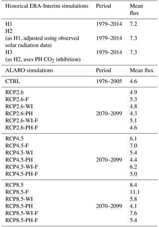
The MEGAN–MOHYCAN model is run at hourly resolution on a $\mathrm{0.1}{}^{\circ }\times \mathrm{0.1}{}^{\circ }$ grid. In its current setup, the model requires the following meteorological input data at hourly resolution: downward solar radiation, cloud cover fraction, air temperature above the surface, dew-point temperature (or relative humidity), and wind speed directly above the canopy. Different climatological input data were used depending on the simulation. Table 1 summarizes all simulations and the corresponding meteorological input. The isoprene emissions for 1979–2014 were obtained by using ERA-Interim ECMWF (European Center for Medium range Weather Forecasts) meteorological fields (Dee et al., 2011) over the above period.

Table 1 Overview of performed simulations. The letter F denotes that the LAI response to CO₂ changes is accounted for based on Zhu et al. (2016) (see text). Simulations with WI account for CO₂ inhibition following Wilkinson et al. (2009) and those with PH follow the Possell and Hewitt (2011) parameterization. Mean isoprene flux over the given periods is expressed in teragrams of isoprene per year.

To account for observed solar radiation changes over Europe we performed a second simulation (H2) where the ERA-Interim downward solar radiation fields are adjusted based on homogenized composite time series of ground-based observations from 56 European sites (Sanchez-Lorenzo et al., 2015). The sites are grouped in five large European regions (central, northern, eastern, southern, and northwestern Europe, Fig. S2). We calculated the seasonally averaged solar radiation according to ERA-Interim at the locations of the observation sites over 1979–2014 and computed their averages ${\stackrel{\mathrm{‾}}{\mathrm{SSR}}}_{\mathrm{ECMWF}}^{i,k}$ over each large region i and each season k. The same procedure is applied for the ground-based observations, ${\stackrel{\mathrm{‾}}{\mathrm{SSR}}}_{\mathrm{obs}}^{i,k}$. We calculate correction factors

$$\begin{array}{}\text{(6)}& f_{i,k}=\mathrm{1}+{\displaystyle \frac{\mathrm{\Delta }\left({\mathrm{SSR}}_{\mathrm{obs}}^{i,k}\right)}{{\stackrel{\mathrm{‾}}{\mathrm{SSR}}}_{\mathrm{obs}}^{i,k}}}-{\displaystyle \frac{\mathrm{\Delta }\left({\mathrm{SSR}}_{\mathrm{ECMWF}}^{i,k}\right)}{{\stackrel{\mathrm{‾}}{\mathrm{SSR}}}_{\mathrm{ECMWF}}^{i,k}}},\end{array}$$

where $\mathrm{\Delta }({\mathrm{SSR}}_{\mathrm{obs}}^{i,k}$) is the seasonal mean anomaly of solar radiation observed in region i, and $\mathrm{\Delta }\left({\mathrm{SSR}}_{\mathrm{ECMWF}}^{i,k}\right)$ is the corresponding anomaly of the ERA-Interim data. The correction factors f_i,k are then applied to the solar radiation fields P of Eq. (4). The ERA-Interim seasonal surface solar radiation anomalies show a fairly good agreement with the corresponding observed anomalies averaged over five large European regions (central, northern, eastern, southern, and northwestern Europe, Fig. S2) and the calculated correlation coefficient is generally higher than 0.8, except in northwestern Europe (0.75). The ERA-Interim data are found to underestimate the observed decadal trends in all regions and seasons, by a factor of 2–3 in spring and summer. The use of the adjusted observation-based solar radiation fields in the MEGAN–MOHYCAN simulations leads to slightly higher trends in the estimated isoprene fluxes over Europe (see Sect. 3), in particular over northwestern Europe.

In order to estimate the impact of climate change, simulations using the regional climate model ALARO were performed. ALARO is the limited-area model version of the ARPEGE-IFS forecast model developed within the ALADIN consortium (Bubnová et al., 1995; ALADIN international team, 1997). These runs were performed following the prescriptions of the international COordinated Regional climate Downscaling EXperiment (CORDEX). Therefore the target domain is the EURO-CORDEX domain (34–70^∘ N, 25^∘ W–50^∘ E, http://www.euro-cordex.net; last access: 15 June 2018) with a horizontal resolution of 12.5 km. As lateral boundary conditions over the European domain, ALARO used the global climate simulations from the CNRM-CM5 model following the guidelines of the fifth Coupled Model Intercomparison Project (CMIP5; Taylor et al., 2011). Validation of ALARO was conducted by comparing observations with model runs forced by realistic boundary conditions from the ERA-Interim reanalysis dataset (Hamdi et al., 2012; De Troch et al., 2013; Giot et al., 2016), and the model was shown to perform in line with other regional climate models (RCMs) of the EURO-CORDEX ensemble over Europe (Giot et al., 2016).

With ALARO we assessed the impact of a changing climate following three RCP scenarios, RCP2.6, RCP4.5, and RCP8.5 (Van Vuuren et al., 2011), which span a range of potential changes in future anthropogenic emissions. The RCP2.6 scenario assumes a peak in radiative forcing at 3.1 W m⁻² (490 ppm CO₂) by midcentury followed by a decline to 2.6 W m⁻² by 2100. In RCP4.5 a moderate increase in radiative forcing to 4.5 W m⁻² is assumed until 2050, with a stabilization thereafter (650 ppm CO₂). In RCP8.5, emissions continue to rise throughout the 21st century with rising radiative forcing leading to 8.5 W m⁻² (1370 ppm CO₂) by 2100 (Van Vuuren et al., 2011). The performed simulations using ALARO meteorology are summarized in Table 1 for 2070–2099 and the results are compared to the control (CTRL) simulation covering 1976–2005. Additional simulations, accounting for the effects of CO₂ inhibition and fertilization, are discussed in Sect. 2.4.

2.3 Leaf area index

Leaf area index is obtained from the MODIS 8-day MOD15A2 (collection 5) composite product generated by using daily Aqua and Terra observations at 1 km² resolution between 2003 and 2014 (Shabanov et al., 2005). Before 2003, the monthly LAI at every grid cell (x) and month (m) is estimated based on the local temperature of the current and previous months:

$$\begin{array}{ll}{\displaystyle }\mathrm{LAI}(x,m)& {\displaystyle }=A(x,m)+B(x,m)\\ \text{(7)}& {\displaystyle }& {\displaystyle }\cdot (\mathrm{0.65}\cdot T(x,m)+\mathrm{0.35}\cdot T(x,m-\mathrm{1}\left)\right),\end{array}$$

with A(x,m) and B(x,m) determined from a linear regression between the monthly MODIS LAI data and the ERA-Interim near-surface temperatures between 2003 and 2014. Note that the slope B(x,m) is set to zero when the correlation between LAI and temperature is poor (r<0.3), and in that case the climatological average LAI over 2003–2014 is used. We use the climatological average of the LAI in our standard future (2070–2099) simulations. The increase in LAI associated with CO₂ fertilization is accounted for in separate simulations (Table 1). Changes in vegetation composition are not considered.

2.4 CO₂ inhibition and fertilization

We account for the direct effect of atmospheric CO₂ concentration changes on isoprene emissions through the activity factor ${\mathit{\gamma }}_{{\mathrm{CO}}_{\mathrm{2}}}$ in Eq. (1). This factor is applied to the historical simulation (H3) and to the ALARO simulations, as shown in Table 1. Two different parameterizations were tested, Wilkinson et al. (2009) (WI) and Possell and Hewitt (2011) (PH). The empirical parameterization by Wilkinson et al. (2009) is given by Eq. (8),

$$\begin{array}{}\text{(8)}& {\mathit{\gamma }}_{{\mathrm{CO}}_{\mathrm{2}}}=I_{\mathrm{smax}}/(\mathrm{1}+(C_i/C_{\star }{)}^h),\end{array}$$

where I_smax=1.344, C_i is the leaf internal CO₂ concentration at non-water-stressed conditions, which is equal to 70 % of the atmospheric CO₂ concentration, $C_{\star }=\mathrm{585}$ ppm, and h=1.4614. The ${\mathit{\gamma }}_{{\mathrm{CO}}_{\mathrm{2}}}$ is equal to 1 at the atmospheric CO₂ concentration of 402.6 ppm. This parameterization was determined empirically based on growth experiments with two aspen tree species (Populus deltoides and P. tremuloides) grown at four different CO₂ concentrations (400, 600, 800, 1200 ppm), and was used to determine the impact of CO₂ inhibition in the future atmosphere (Heald et al., 2009).

The parameterization of Possell and Hewitt (2011) is obtained by an empirical nonlinear least-squares regression, based on a combination of laboratory and field observations obtained from 10 different studies on various plant species including tropical and temperate tree species as well as herbaceous plant species

$$\begin{array}{}\text{(9)}& {\mathit{\gamma }}_{{\mathrm{CO}}_{\mathrm{2}}}=a/(\mathrm{1}+a\cdot b\cdot C),\end{array}$$

where C is the atmospheric CO₂ concentration, and a=8.9406 and b=0.0024 ppm⁻¹ are fitting parameters; ${\mathit{\gamma }}_{{\mathrm{CO}}_{\mathrm{2}}}$ is equal to 1 at the CO₂ concentration of 370 ppm.

For CO₂ concentrations higher than 380 ppm the PH parameterization induces a relatively stronger inhibition (1 to 0.3) compared to the WI parameterization (1 to 0.4) (Fig. 1). The parameterizations result in similar ${\mathit{\gamma }}_{{\mathrm{CO}}_{\mathrm{2}}}$ values at concentrations corresponding to the historical simulations and to the RCP2.6 scenario, but differ by around 20 % for the RCP4.5 and RCP8.5 scenarios. In both schemes the inhibition factor behaves linearly at very high CO₂ levels. Here we use the more recent PH parameterization in the historical H3 simulation (Table 1). Both parameterizations are tested in the case of ALARO simulations, thus providing a range of the CO₂ inhibition effect in the projected emission estimates.

Figure 1 Dependence of the CO₂ inhibition factor on ambient CO₂ concentrations following the Wilkinson et al. (2009) and Possell and Hewitt (2011) parameterizations. The vertical bands show the ranges of CO₂ concentrations for the historical simulations and following the different RCP scenarios.

Lastly, we estimated the effect of CO₂ fertilization on the projected emissions through the expected enhancement in leaf biomass densities and LAI based on a recent study (Zhu et al., 2016). Using long-term (1982–2009) satellite LAI records and ecosystem models, Zhu et al. (2016) obtained a widespread increase in LAI over the majority of vegetated areas on the global scale and attributed the major part of the observed greening trends to CO₂ fertilization. This is crudely parameterized here as a linear LAI increase of 15 % per 100 ppm of CO₂ concentration (Table 1). Dynamical vegetation models, e.g., ORCHIDEE (Krinner et al., 2005; Messina et al., 2016), would be required in order to provide a more mechanistic simulation of the LAI variations and of the distribution and structure of the natural vegetation, but this lies beyond the scope of the present study. Note, however, that dynamical vegetation models have identified weaknesses related to the use of a limited number of static plant functional types, and to the poor representation of species competition (Scheiter et al., 2013).

3 Historical isoprene estimates (1979–2014)

Figure 2 illustrates the mean distribution of isoprene emissions for the simulation H3 over 1979–2014 (Table 1). This simulation incorporates the effect of climate on the emissions based on ERA-Interim fields, but with adjusted solar radiation fields based on observations, as described in Sect. 2.2, and accounts for the CO₂ inhibition based on Possell and Hewitt (2011). The map shows higher isoprene emissions in the Mediterranean countries and over European Russia. The relatively high isoprene emission in the Mediterranean countries is mainly associated with warmer temperatures and stronger radiation fluxes, as well as with the high isoprene emission capacity from the vegetation compared to the rest of Europe: e.g., some oak (Quercus) species common in the Mediterranean regions have a strong emission capacity (Karl et al., 2009). In European Russia the densely forested regions are characterized by a high LAI during summertime (Fig. S3), resulting in high simulated isoprene emissions. The distribution of isoprene emissions is very similar in both the H1 and H2 simulations (Table 1) and is not shown here.

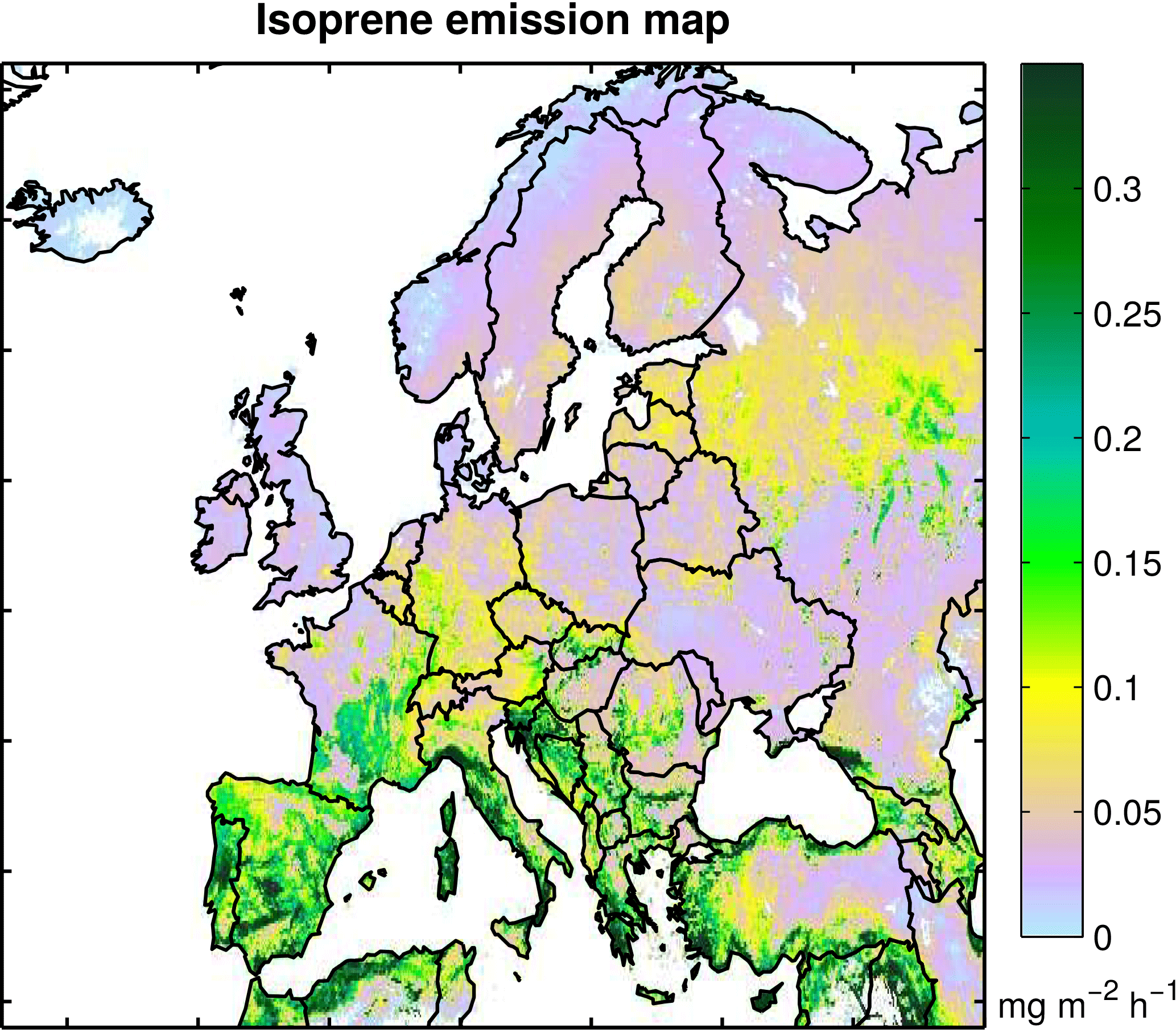
Figure 2 Isoprene emission map from the H3 simulation (Table 1), showing the distribution of isoprene emissions (in mg m⁻² h⁻¹) using the ERA-Interim reanalyses for 1979–2014.

Figure 3 Annual isoprene emission and emission trends between 1979 and 2014 (in % per year) over the European domain (34–70^∘ N, 25^∘ W–50^∘ E), obtained from the historical simulations (Table 1). Mean annual summer temperature and solar radiation (PAR) obtained from ERA-Interim (ECMWF) reanalyses over the same period are shown in the middle and lower panels, respectively.

Also, in terms of interannual variability the three historical simulations result in very similar estimates (Fig. 3), and a relatively uniform increase of isoprene emissions over 1979–2014. The simulation H2 exhibits a slightly higher emission trend (1.34 % yr⁻¹) compared to H1 (1.09 % yr⁻¹). Indeed, as can be seen in Fig. S1 the interannual variation of the observed downward solar radiation fields is very similar to the variation of the ERA-Interim fields, with correlations higher than 0.7 for all regions and seasons, but the observed solar radiation records exhibit slightly stronger positive trends than the ERA-Interim data. This is the case for all seasons and regions, and in particular for central Europe, where observed solar radiation trends are much stronger than the respective trends modeled by ECMWF reanalyses (e.g., 2.9 vs. 0.9 % decade⁻¹ in summer). Due to the higher-than-1 ${\mathit{\gamma }}_{{\mathrm{CO}}_{\mathrm{2}}}$ in the PH parameterization for CO₂ levels lower than 380 ppm (Fig. 1), the emissions are moderately increased until 1990 in the H3 simulation, and therefore the calculated trend (0.76 % yr⁻¹) is lower than in the H1 and H2 simulations. The trends are stronger (up to 2 % yr⁻¹) in eastern and central Europe, and weaker or close to zero over the United Kingdom, the Scandinavian countries, and Spain. The interannual variability of temperature and solar radiation explains most of the flux variability and increasing isoprene trend.

Figure 4 Annual isoprene emissions normalized to the emission in 1979 for 16 European countries. In the upper left corner of every panel the total isoprene emissions for every country in 1979 are given as well as the emission trend over 1979–2014. The emissions are obtained from the H3 simulation (Table 1).

As shown in Fig. 4, the interannual variability of emissions can strongly differ among countries. European Russia (793–2466 Gg), Turkey (645–944 Gg), Spain (569–856 Gg), France (312–771 Gg), and Italy (354–621 Gg) are among the most emitting regions. The interannual variability in the isoprene emissions generally reflects the variability in temperature and solar radiation (Fig. S4), and therefore isoprene maxima are typically observed during years with particularly hot summers. The exceptional heat wave in central Europe in summer 2003 induced a pronounced isoprene emission peak in France and Germany, with emissions about twice as high as in normal years. The emission peak modeled over European Russia and Belarus in 2010 is associated with a summer heat wave (Barriopedro et al., 2011). Moreover, cold summers with weak solar radiation result in reduced isoprene emissions. For instance, the cold summer of 1987 in Scandinavia and the cold summer of 1993 over all of Europe (Fig. S4) lead to low isoprene emission in these regions (Figs. 3 and 4). Overall, the strong interannual variability in northern European countries, and the very weak variability in Mediterranean countries reflect the interannual variations in summer temperature and solar radiation (Fig. S4).

The calculated emission trends are strongest in central and eastern Europe, reflecting the strongest trends in temperature and radiation (Figs. 3 and S4). For most central and eastern European countries isoprene emissions increase, with trends higher than 1 % yr⁻¹, whereas the trend is often lower than 1 % yr⁻¹ for most northern and Mediterranean countries. The strongest isoprene trend is simulated over Ukraine (1.5 % yr⁻¹).

4 Evaluation of MEGAN–MOHYCAN flux estimates

4.1 Comparison to bottom-up inventories and top-down estimates

In comparison to other bottom-up isoprene inventories, the MEGAN–MOHYCAN estimated emissions are generally lower. Averaged over 1980–2009 in the same EURO-CORDEX domain, our estimates amount to 7.3 Tg yr⁻¹, and are by 22 % lower than in the MEGAN-MACC inventory (9.4 Tg yr⁻¹, Sindelarova et al., 2014), and about 3 times lower than in the GUESS-ES model (20.1 Tg yr⁻¹, Arneth et al., 2007; Niinemets et al., 1999). Similarly, satellite-based isoprene emission estimates, obtained using observations of formaldehyde, a high-yield isoprene oxidation product, indicate slightly higher isoprene emissions with respect to our estimates. For instance, an inversion study constrained by OMI (Ozone Monitoring Instrument) formaldehyde observations over a decade (2005–2014) suggested top-down isoprene emissions amounting to 8.4 Tg yr⁻¹, i.e., 20 % higher than in the a priori MEGAN–MOHYCAN inventory (Bauwens et al., 2016). In the same line, an independent study using OMI formaldehyde observations from 2005 inferred an average increase of isoprene emissions by 11 % over Europe and emission decreases of 20–40 % in southern Europe with regards to their a priori MEGAN estimate (Curci et al., 2010).

In the following sections, the isoprene emissions estimated by the H3 simulation (Table 1) are compared directly to isoprene flux measurements in Europe. Section 4.2 presents a comparison of modeled isoprene emissions with campaign-averaged isoprene fluxes measured at seven different locations. Section 4.3 investigates the ability of the model to reproduce the temporal variations as observed in Vielsalm (Belgium) and in Stordalen (Sweden).

4.2 Campaign-averaged isoprene fluxes

Figure 5 shows the monthly averaged midday fluxes estimated in the H3 simulation at the model grid cells corresponding to the location of nine field campaigns (Acton et al., 2016; Baghi et al., 2012; Brilli et al., 2014; Davison et al., 2009; Holst et al., 2010; Kalogridis et al., 2014; Laffineur et al., 2011, 2013; Spirig et al., 2005), using either the MEGAN emission factors or using local emission factors (see further below).

Differences between field measurements and modeled data were expected, since the local vegetation around the measurement site differs from the heterogeneous vegetation mix of the model grid cell (in addition, the effect of the footprint on the flux measurements is also not taken into account by the model). The PFT fractional areas of the local vegetation are compared to the model PFT fractions of the corresponding grid cell in Fig. S5. Many field campaigns were conducted in forests whereas the corresponding model grid cells consist for a large part (15 to 91 %) of low isoprene-emitting PFTs such as crops, grass, and bare soil. At these sites (ECHO, Lochristi, Haute Provence, and Bosco Fontana), this discrepancy explains the large underestimation of model estimates using MEGAN emission factors. At Castelporziano, however, the relatively open local landscape is not well represented by the $\mathrm{0.1}{}^{\circ }\times \mathrm{0.1}{}^{\circ }$ vegetation map, which suggests a substantial fraction of needleleaf forest, partly explaining the emission overestimation at this location.

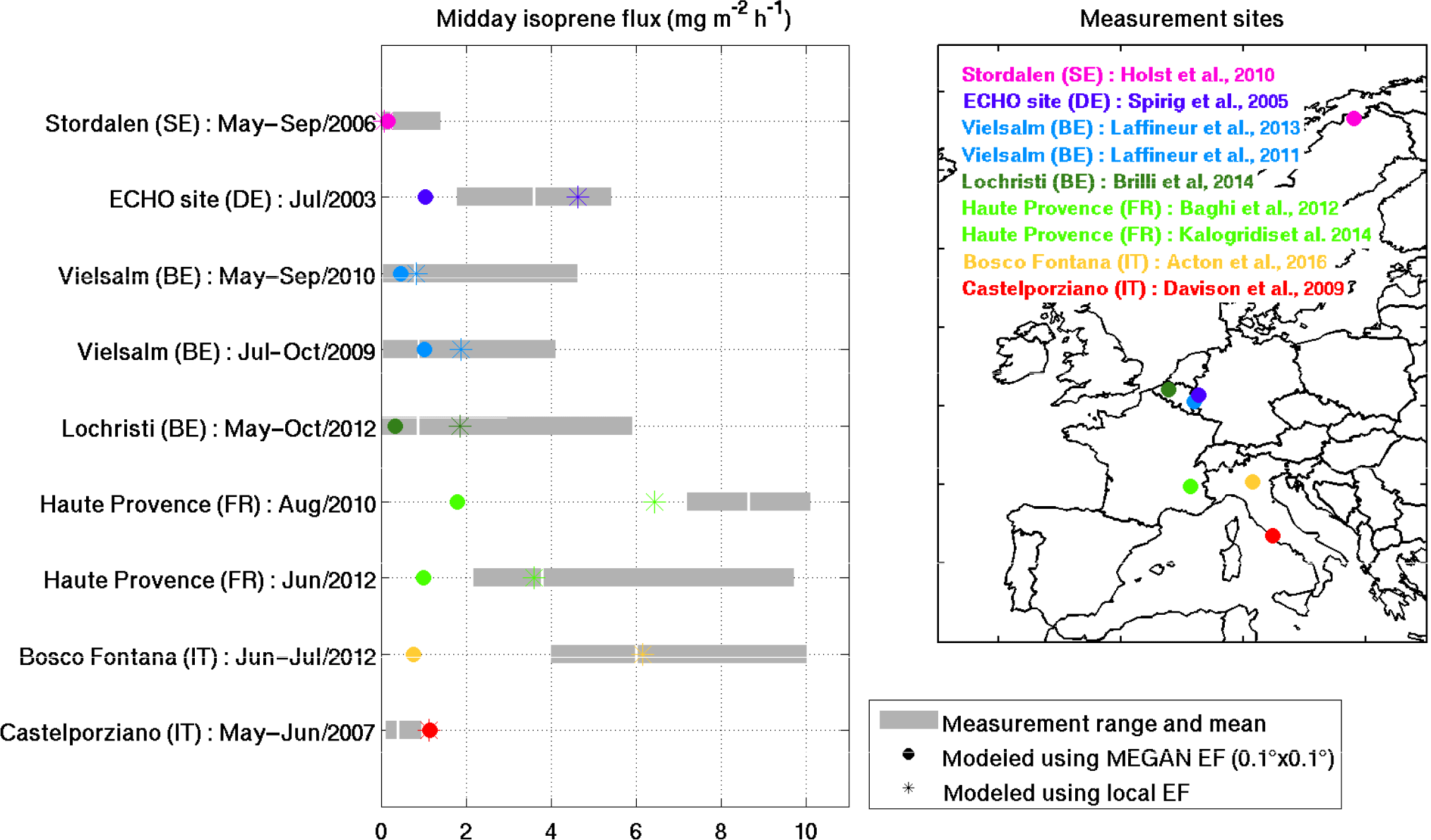
Figure 5 Modeled and measured isoprene midday fluxes from nine field campaigns over Europe. The circles indicate the monthly mean emissions modeled in the $\mathrm{0.1}{}^{\circ }\times \mathrm{0.1}{}^{\circ }$ cell including the measurement site using the emission factors of MEGAN–MOHYCAN. The stars denote the modeled fluxes using local emission factors (see text for details). The gray bands show the range of measured midday fluxes observed during the field campaigns. The average midday flux is shown in white.

In order to correct for this effect, we re-calculated the model isoprene fluxes using local emission factors. These emission factors are based on the local PFT fractions (Fig. S5) combined with the standard emission factors (SEFs) given for the different PFTs in Guenther et al. (2012): 10 mg m⁻² h⁻¹ for the broadleaf deciduous sites (ECHO, Lochristi, Haute Provence, Bosco Fontana), 5.3 mg m⁻² h⁻¹ at Vielsalm, 1.8 mg m⁻² h⁻¹ at Castelporziano, and 1.6 mg m⁻² h⁻¹ in Stordalen. Overall, the use of local emission factors significantly improves the model performance and reduces the average bias for all sites from −70 to +5 % (Fig. 5).

Note, however, that local emission factor estimates based on SEFs defined for broad PFTs (Guenther et al., 2012) are still crude approximations for the local SEFs. For instance, the SEF at the ECHO site is likely too high since it is dominated by non-isoprene emitters such as Fagus sylvatica and Betula pendula (Karl et al., 2009). Similarly, the vegetation at Castelporziano is a mixture of low-isoprene-emitting species like Quercus ilex and Arbutus unedo (0.1 µg g${}_{\mathrm{DW}}^{-\mathrm{1}}$ h⁻¹, where DW denotes dry weight of leaf biomass) and non-isoprene emitters such as Erica multiflora, Rosmarinus officinalis, and Phillyrea angustifolia, and therefore the SEF calculated assuming a large fraction of strongly emitting shrubs is likely too high. For Vielsalm, a local SEF of 2.88 mg m⁻² h⁻¹ is used, adjusted to minimize the average bias between the model and the observations in 2010 (see next section).

The model overestimation at the poplar plantation in Lochristi (Fig. 5) is unexpected, given that Populus sp. is a strong isoprene emitter (Karl et al., 2009). However, the plantation was coppiced 6 months before the measurements, and new shoots started to sprout only in May 2012 (Brilli et al., 2014), possibly explaining the difference between the modeled and the measured isoprene fluxes at that site (Fig. S6).

At Bosco Fontana, where a mixture of strong emitters (Quercus robur and Quercus rubra) and low emitters (Quercus cerris and Carpinus betulus) is present, a good agreement between modeled and measured flux is obtained, suggesting that the SEF of 10 mg m⁻² h⁻¹ is representative for this landscape. At the site in Haute Provence, dominated by a strong isoprene emitter (Quercus pubescens), an excellent agreement is obtained for the field campaign in June 2012 (Kalogridis et al., 2014), whereas the model is somewhat too low in August 2010 (Baghi et al., 2012).

4.3 Evaluation of temporal variations

The model potential to capture temporal flux variations is evaluated against flux measurements at the Vielsalm site located in a temperate mixed forest in the Belgian Ardennes (50.30^∘ N, 5.99^∘ E). The site consists of a mixture of evergreen needleleaf trees (mainly Pseudotsuga menziesii, Picea abies, and Abies alba) and deciduous broadleaf tree species (mainly the non-isoprene emitter Fagus sylvatica). Those tree species are generally weak isoprene emitters, explaining the low local SEF of 2.88 mg m⁻² h⁻¹. The main isoprene emitters are likely green needleleaf trees, especially the Abies alba (Pokorska et al., 2012).

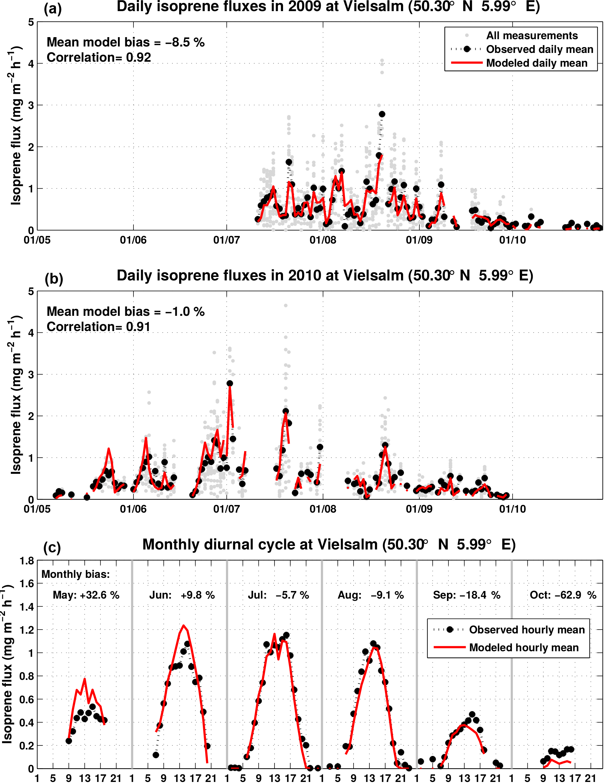
Figure 6 Modeled (red) and measured (black and gray) daily isoprene fluxes in Vielsalm in 2009 (Laffineur et al., 2011) and in 2010 (Laffineur et al., 2013). The model (H3 simulation) uses the local emission factor (SEF = 2.88 mg m⁻² h⁻¹). The lower panel shows the monthly diurnal cycle for the modeled (red) and measured (black) isoprene fluxes, as well as the monthly bias.

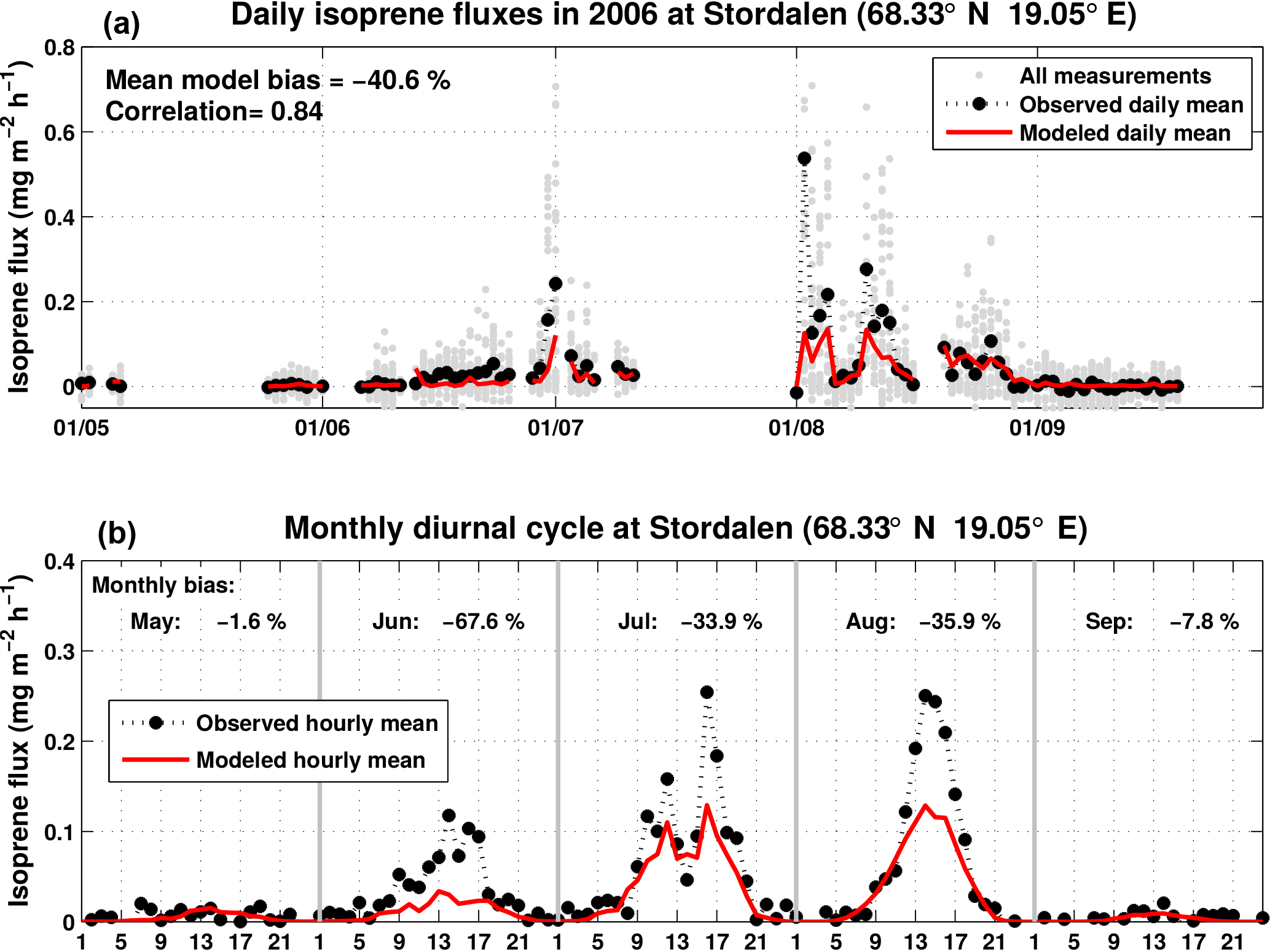
Figure 7 Modeled (red) and measured (black and gray) daily isoprene fluxes in Stordalen in 2006 (Holst et al., 2010). The model (H3 simulation) uses the local emission factor (SEF = 1.6 mg m⁻² h⁻¹). The lower panel shows the monthly diurnal cycle for the modeled (red) and measured (black) isoprene fluxes.

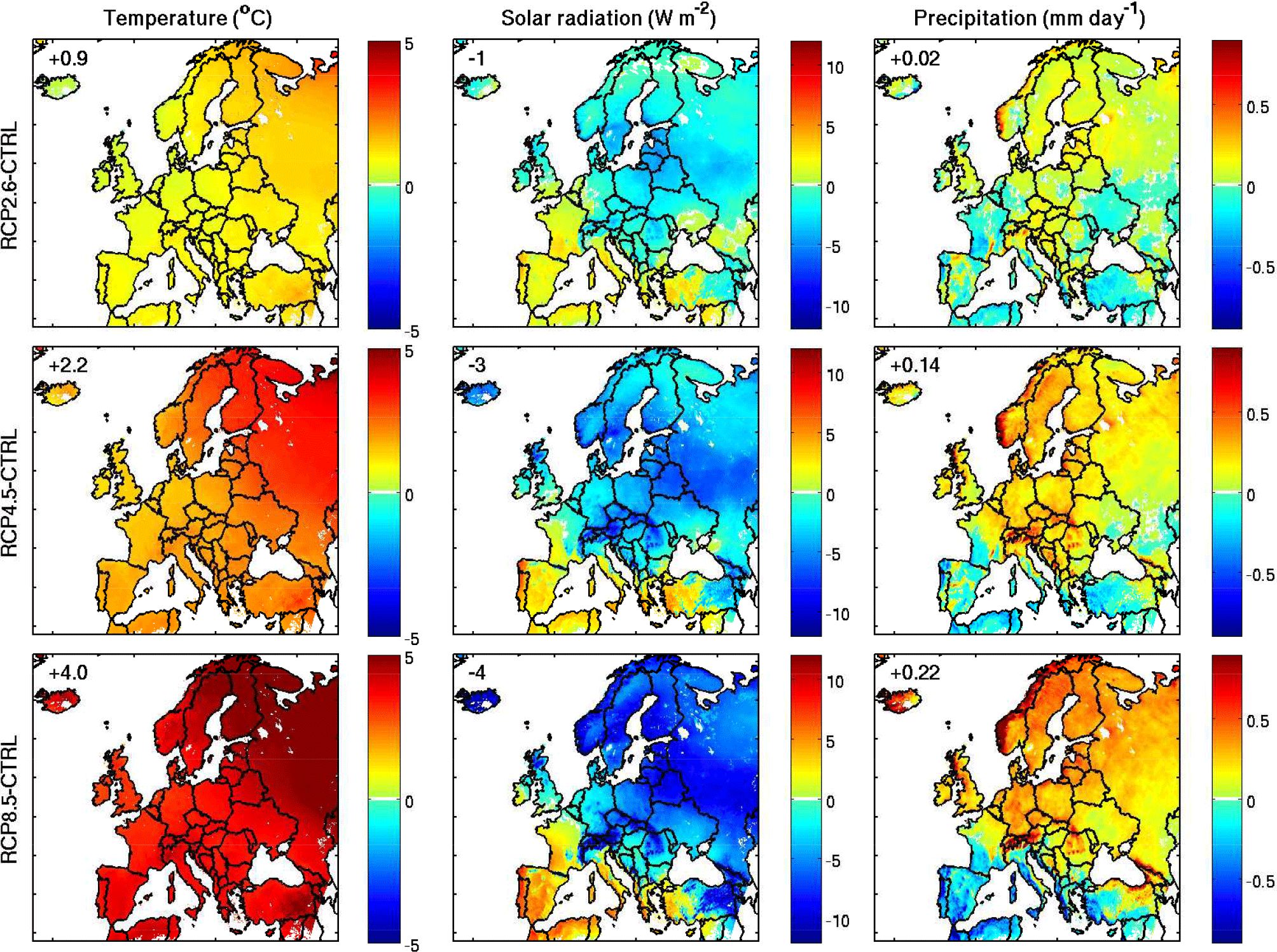
Figure 8 Absolute difference between the projected future and control simulations for temperature, surface shortwave radiation, and precipitation averaged over 2070–2099 following different RCP scenarios. The mean values for each variable over the domain are given inside each panel.

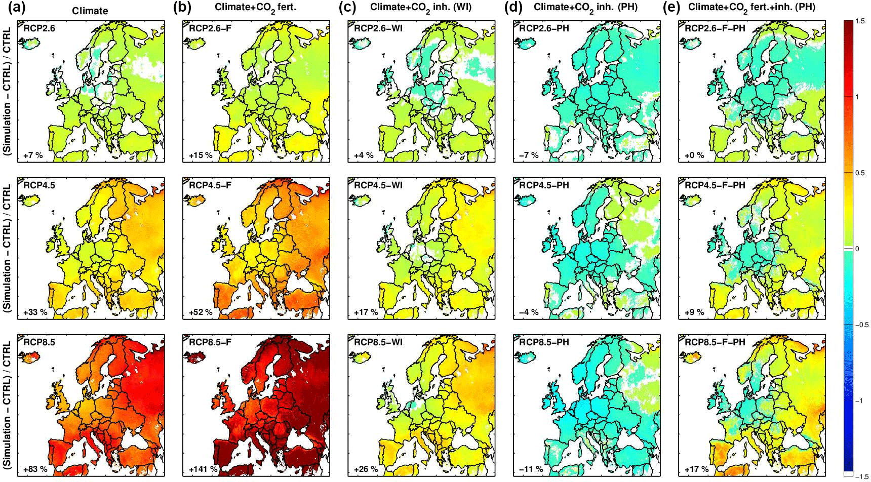
Figure 9 Relative differences in isoprene emissions between the control ALARO simulation (CTRL) and the three RCP scenarios considering the effect of (a) climate (first column), (b) climate and CO₂ fertilization (second column), (c) climate and moderate CO₂ inhibition based on Wilkinson et al. (2009) (third column), (d) climate and strong CO₂ inhibition based on (Possell and Hewitt, 2011) (fourth column), and (e) climate, fertilization, and inhibition based on (Possell and Hewitt, 2011) (last column). The names of the simulations are given in the upper corner of each panel (see Table 1), and in the lower corner is given the relative change for the whole domain compared to the control simulation (CTRL), for which the mean isoprene flux is estimated at 4.6 Tg yr⁻¹ (Table 1).

Figure 10 Comparison of our results to European (a) and global (b) changes in projected isoprene emissions predicted by different studies. The different colors indicate the driving parameters considered in the various simulations. Note that often several simulations are shown for the same study, to represent the impact of different parameters or climate scenarios assumed. The periods are end-of-century for all studies except otherwise stated.

The flux measurements used were obtained by disjunct eddy covariance by mass scanning technique during two field campaigns at the Vielsalm site: July–October 2009 (Laffineur et al., 2011), and May–September 2010 (Laffineur et al., 2013). The isoprene measurements were performed with an hs-PTR-MS (proton transfer reaction mass spectrometer, Ionicon, Innsbruck, Austria). Ambient air was continuously sampled at the top of a tower at a height of 52 m a.g.l. The instrument performs one measurement of isoprene fluxes every 2 s, and half-hourly averages are used for comparison with the model.

Figure 6 displays the evolution of the daily averaged measured and modeled fluxes (panels a and b) as well as their monthly averaged diurnal cycles (panel c). The model averages are calculated with the same temporal sampling as the observations. Both the day-to-day and the diurnal variability are well represented by the model for this site, as reflected by the high correlation coefficients of 0.92 for 2009 and 0.91 for 2010. Whereas the overall bias is small for both field campaigns (−8.3 % for 2009 and −0.8 % for 2010), the modeled seasonal pattern differs from the observed fluxes. The model is biased highly in May (+33 %) and June (+10 %), but it is biased low in September (−18 %) and October (−63 %). A possible explanation for this discrepancy might be that the leaf age factor described in Eq. (5), i.e., the emission from new and growing leaves, might be overestimated, whereas the emission from senescent leaves might be underestimated. It should be noted that the activity factors γ_P and γ_T have their own uncertainties which might also impact the modeled seasonal variation.

A second model validation is performed for a sub-arctic wetland ecosystem at Stordalen in northern Sweden (68.33^∘ N, 19^∘ E, 351 m a.s.l.), 200 km north of the Arctic Circle (Ekberg et al., 2009; Holst et al., 2010). The region is characterized by a short but intensive growing season (from mid-May to mid-September) and is influenced by discontinuous permafrost conditions affecting surface hydrology and, thus, the growth conditions of the vegetation. The vegetation in the vicinity of the measurement tower was dominated by species such as Eriophorum ssp., Carex ssp. and Sphagnum ssp., all known to be low isoprene emitters (Ekberg et al., 2009, 2011).

Isoprene was measured using a hs-PTR-MS, which was combined with a sonic anemometer to estimate ecosystem-scale fluxes using disjunct eddy covariance. Measurements were taken at a height of 2.95 m a.g.l. (vegetation height ca. 50 cm) and fluxes from May to September 2006 reported at a temporal resolution of 30 min (Ekberg et al., 2009; Holst et al., 2010). For isoprene fluxes, the mean estimated error (2σ) was found to be 0.03 mg m⁻² h⁻¹.

The daily averaged observed and modeled fluxes as well as the diurnal cycles of fluxes are shown in Fig. 7. The model is biased low by ca. 40 % on average over the campaign, possibly suggesting an underestimation of the SEF used in the calculation (1.6 mg m⁻² h⁻¹) for arctic C₃ grass (Guenther et al., 2012). However, the model is able to capture the day-to-day variability (correlation coefficient of 0.84) in spite of the low fluxes at that site, frequently of the order of (or even lower than) the estimated error on the fluxes. The low bias of the model might be partly due to a low bias in the LAI values from MODIS used in the model, equal to ca. 0.88 at that site, to be compared with locally measured LAI reaching up to 3.5 at the most dense spots of the wetland sedges. In addition, the MEGAN algorithm might not be optimal for this subarctic vegetation type. As proposed by Ekberg et al. (2009), vegetation in this area is especially well adapted to survive under conditions of short active seasons. The subarctic sedges start photosynthesizing in early spring under still cool temperatures, possibly resulting in isoprene emission induction occurring sooner than in other extratropical ecosystems. This hypothesis is supported by the stronger negative bias in June (−68 %) compared to July and August (ca. −35 %).

5 Projected isoprene fluxes (2070-2099)

5.1 Future climate simulated with ALARO

A comparison between the control ALARO (CTRL, 1976–2005, Table 1) and the historical ERA-Interim surface temperature and solar radiation fields is presented and discussed in the Supplement (Fig. S7). The use of the ALARO control fields results in lower mean isoprene fluxes by 37 % over the domain (Table 1), caused by a negative bias of the ALARO surface temperature fields compared to the ECMWF reanalysis. The CTRL fields are, however, not used here for emission estimation, but as a reference with which the projected isoprene emissions (2070–2099) will be compared. Surface temperature, precipitation, and surface shortwave radiation for the different RCP scenarios are compared to the CTRL fields in Fig. S8.

The absolute difference between the projected (2070–2099) and the control (1976–2005) mean temperature, solar radiation, and precipitation over the European domain, as simulated with the ALARO model for the climate scenarios (Table 1), are displayed in Fig. 8. An average temperature increase of 0.9, 2.2, and 4 ^∘C is found for RCP2.6, RCP4.5, and RCP8.5, respectively, with respect to the control simulation. The change in temperature presents a similar geographic distribution for the three scenarios, with the strongest temperature increases predicted over European Russia and Scandinavia. The simulated pattern as well as the range of temperature changes are consistent with results from other EURO-CORDEX model simulations (Jacob et al., 2014) and projections from the Coupled Model Intercomparison Project (CMIP5; Cattiaux et al., 2013). The intercomparison shows that the largest model disagreements in summer occur in France and in the Balkans, suggesting a higher uncertainty for temperature projections in these regions.

The mean downward solar radiation is decreased over the domain, by up to −4 W m⁻² for the RCP8.5 simulation compared to the control simulation. This average decrease is due to the combination of higher radiation in southern European countries and France (up to +8 W m⁻²) and decreases elsewhere (up to −10 W m⁻²). The amplitude of the expected changes in solar radiation and the simulated pattern are in line with results from the EURO-CORDEX ensemble (Jerez et al., 2015; Bartok et al., 2016). Note, however, that the different climate simulations in the EURO-CORDEX ensemble show large discrepancies over France, central Europe, and the coastal areas of Italy, Greece, and Turkey, underlining a higher uncertainty in projections of solar radiation in these regions (Jerez et al., 2015).

Finally, the model predictions suggest a drier Mediterranean and wetter northern and eastern Europe (Fig. 8). This pattern agrees reasonably well with previous studies (Frei et al., 2006; Lacressonnière et al., 2014) and with the EURO-CORDEX ensemble (Jacob et al., 2014). The latter suggests a robust increase in precipitation in central and northern Europe (up to 25 %), as well as a drop in precipitation in southern Europe (by up to 25 %). Note that according to the EURO-CORDEX ensemble, future precipitation projections show strong variability across different simulations at the 45^∘ N latitude band, including southern France, northern Italy, and central Romania (Jacob et al., 2014).

5.2 Effects of climate, CO₂ inhibition, and fertilization on isoprene flux estimates

The impact of climate change on annual isoprene emissions according to the different RCP scenarios, upon neglecting the CO₂ inhibition effect, is shown in the first column of Fig. 9. Whereas the RCP2.6 simulation suggests very weak changes in isoprene emissions (lower than 20 %), RCP4.5 and RCP8.5 indicate local emission increases reaching 40 and 110 %, respectively. In all simulations the strongest increase is found in southern Europe, European Russia, and Finland. This pattern, consistent with independent simulations (Lacressonnière et al., 2014), reflects the patterns of changes in temperature and solar radiation. The higher isoprene emissions in northeastern Europe are mainly a result of the strongly increased temperatures, and are somewhat counteracted by the decreasing solar radiation. In southwestern Europe the higher emissions are due to the combined effect of moderate temperature increases and cloud cover decreases.

When considering the effect of CO₂ fertilization, we obtained a significant enhancement of the emissions, by +15 % (RCP2.6), +52 % (RCP4.5), and +141 % (RCP8.5), compared to the control simulation, and an increase by +8 % (RCP2.6), +15 % (RCP4.5), and +32 % (RCP8.5) compared to the simulation accounting only for climate effects (Fig. 9, Table 1). The combined effect of climate change and CO₂ inhibition is also shown in Fig. 9. Since both are of similar magnitude, but of opposite sign, considering both effects leads to isoprene fluxes similar to the control emissions. The strength of the CO₂ inhibition, however, is different for the two parameterization schemes tested here (Wilkinson et al., 2009; Possell and Hewitt, 2011). In comparison to the control simulation, total projected isoprene fluxes are 11 % lower and 26 % higher in the RCP8.5 scenario following Possell and Hewitt (2011) or Wilkinson et al. (2009), respectively. For the other RCP scenarios, the simulated changes in isoprene emission range between −7 and 17 %. Note that the spatial pattern of the emission change is not influenced by introducing the CO₂ inhibition effect since CO₂ is uniformly distributed. When incorporating all the above effects, the end-of-century modeled isoprene fluxes are found to range either between 0 % (RCP2.6) and +17 % (RCP8.5) (using Possell and Hewitt (2011)) or between 11 and 65 % (using Wilkinson et al. (2009), not shown), with respect to the control fluxes. Note, however, that recent studies suggest that the CO₂ inhibition of isoprene is reduced at high temperatures and therefore it may not have a large influence in the warmer Europe predicted in future climate scenarios (Sun et al., 2013; Potosnak, 2014).

Precipitation plays only a minor role in most regions, although the drier future summers simulated for Mediterranean regions should lead to enhanced soil moisture stress, which is believed to inhibit isoprene emission (Guenther et al., 2006), and therefore tend to decrease the fluxes. As the present study neglects the effect of soil moisture on isoprene fluxes, the present and future fluxes are likely to be somewhat overestimated, in particular over southern Europe. In this region the increasing temperatures and the decreasing precipitation trends (Haren et al., 2013; Vicente-Serrano et al., 2014 and Fig. 8) should result in enhanced soil moisture stress, possibly causing a decline of isoprene fluxes over time. However, the influence of soil moisture stress on isoprene fluxes is still highly uncertain; for example, the MEGAN parameterization implemented with soil moisture fields from ECMWF reanalyses has been found to overestimate this effect over arid and semiarid regions (Bauwens et al., 2016).

Our simulations predict isoprene emission changes falling within the range of previous studies, i.e., between +90 % (Young et al., 2009) and −55 % (Squire et al., 2014) on the global scale, and between +85 % (Andersson and Engardt, 2010) and −30 % (Arneth et al., 2008) over Europe (Fig. 10). The large dispersion of the different estimates of Fig. 10 is, to a large extent, explained by the diversity of model setups, namely the climate scenario, the study period, and most importantly, the choice of driving parameters which are allowed to vary (i.e., the climate fields, the CO₂ activity factor, and/or the vegetation distribution). The increase in isoprene emission as a result of climate change of +70 % (Pacifico et al., 2012) globally and of +85 % (Andersson and Engardt, 2010) over Europe are very close to the predicted emission change in our study when only climate changes are considered. Weaker emission changes are induced when incorporating the CO₂ inhibition effect, being between −10 % (Heald et al., 2009) and +25 % (Wu et al., 2012) compared to present-day emissions, in good consistency with the emission changes simulated in the present study.

Considering future changes in vegetation induces an additional decrease or increase in isoprene emissions depending on the simulation setup. The use of a dynamical vegetation model generally leads to higher isoprene flux estimates due to the increasing biomass as result of rising temperatures, radiation, and CO₂ fertilization (Arneth et al., 2008; Heald et al., 2009). Overall, most studies using a dynamical vegetation model agree on a relatively strong flux increase in the wide range of 27 % (Lathière et al., 2005) to 360 % (Heald et al., 2009). Human-induced land use changes generally cause less drastic emission changes (Zhu et al., 2016). Significant cropland expansion is likely to result in lower isoprene fluxes globally, at most 41 % lower than present-day emissions (Ganzeveld et al., 2010; Hardacre et al., 2013; Lin et al., 2016; Squire et al., 2014; Wiedinmyer et al., 2006). A recent study reported that, globally, human-induced land cover change is expected to have a more significant impact than natural vegetation changes, leading to a relative decrease of future isoprene emissions up to 33 % (Hantson et al., 2017). Note, however, that afforestation is expected to be the dominant land use change over Europe, and therefore the combination of natural and human-induced vegetation changes could induce a significant increase in isoprene emission of up to 40 % (Beltman et al., 2013; Hendriks et al., 2016). The application of land use change scenarios (e.g., those of the ALARM project, Settele et al., 2005) to projected isoprene emission estimates with MEGAN–MOHYCAN will be carried out in future work.

6 Conclusions

In this study we simulated high-resolution (0.1^∘, hourly) isoprene emission estimates above Europe over 1979–2014 using the MEGAN–MOHYCAN model and ERA-Interim reanalysis fields. The mean isoprene flux over the entire period is estimated to be 7.3 Tg yr⁻¹. As a result of the climate change, a positive trend of ca. 1.1 % yr⁻¹ is simulated over Europe, with strongest trends over eastern and northeastern Europe (up to 2–3 % yr⁻¹). The warming temperatures and the changing solar radiation are the main drivers, determining the interannual variability and trends in isoprene fluxes. The trend is moderately increased (1.3 %) when the input solar radiation reanalysis fields are adjusted to match observed solar radiation over Europe, due to a stronger solar brightening trend in the observations than in the reanalysis fields. Further, when the effect of CO₂ inhibition is considered in the model simulations, the trend is reduced and is estimated to be 0.76 % yr⁻¹ over Europe. Comparison with flux campaign measurements performed at seven European sites shows that the simulated fluxes reliably reproduce the day-to-day variability and the diurnal cycle of the observations, lending strong confidence to the MEGAN–MOHYCAN model and its input variables.

The projected (2070–2099) simulations based on the ALARO meteorology suggest higher temperatures over the entire domain and stronger irradiance in southwestern Europe. Driven by the changing climate only, isoprene emissions are predicted to increase by 7, 33, and 83 %, in the RCP2.6, RCP4.5, and RCP8.5 scenarios, respectively, with respect to the control simulations covering the period 1976–2005. The CO₂ fertilization and CO₂ inhibition effects are of opposite sign, and taken together, the end-of-century European isoprene emissions are calculated to increase by 0–11, 9–35, and 17–65 % according to the RCP2.6, RCP4.5, and RCP8.5 scenarios, respectively (Table 1). The impact of these processes is still largely uncertain.

Finally, although the use of the MEGAN model to simulate the short-term isoprene emission response has been robustly tested against numerous campaign measurements of short duration, the long-term emission response to environmental changes bears large uncertainties. These uncertainties are associated with the model components, and likely with other unaccounted-for control factors, and their assessment is currently hampered by the lack of long-term isoprene measurements. The estimates provided in this study could be improved in future work, for example using meteorological output from more than one climate model, using alternative long-term leaf area index datasets, and especially through the coupling with a dynamical vegetation model, in order to better evaluate model uncertainties related to climate and vegetation changes and to better represent the complex and numerous biosphere–climate interactions. Moreover, the effects of soil moisture stress on isoprene emissions should also be considered, as climate scenarios frequently predict a higher occurrence of droughts in the future.