the Creative Commons Attribution 4.0 License.
the Creative Commons Attribution 4.0 License.
 | 14 Sep 2018
On estimating the gross primary productivity of Mediterranean grasslands under different fertilization regimes using vegetation indices and hyperspectral reflectance
Manuel Campagnolo
Joana Faria
Carla Nogueira
Maria da Conceição Caldeira
We applied an empirical modelling approach for gross primary productivity (GPP) estimation from hyperspectral reflectance of Mediterranean grasslands undergoing different fertilization treatments. The objective of the study was to identify combinations of vegetation indices and bands that best represent GPP changes between the annual peak of growth and senescence dry out in Mediterranean grasslands.
In situ hyperspectral reflectance of vegetation and CO2 gas exchange measurements were measured concurrently in unfertilized (C) and fertilized plots with added nitrogen (N), phosphorus (P) or the combination of N, P and potassium (NPK). Reflectance values were aggregated according to their similarity (r≥90 %) in 26 continuous wavelength intervals (Hyp). In addition, the same reflectance values were resampled by reproducing the spectral bands of both the Sentinel-2A Multispectral Instrument (S2) and Landsat 8 Operational Land Imager (L8) and simulating the signal that would be captured in ideal conditions by either Sentinel-2A or Landsat 8.
An optimal procedure for selection of the best subset of predictor variables (LEAPS) was applied to identify the most effective set of vegetation indices or spectral bands for GPP estimation using Hyp, S2 or L8. LEAPS selected vegetation indices according to their explanatory power, showing their importance as indicators of the dynamic changes occurring in community vegetation properties such as canopy water content (NDWI) or chlorophyll and carotenoids ∕ chlorophyll ratio (MTCI, PSRI, GNDVI) and revealing their usefulness for grasslands GPP estimates.
For Hyp and S2, bands performed as well as vegetation indices to estimate GPP. To identify spectral bands with a potential for improving GPP estimates based on vegetation indices, we applied a two-step procedure which clearly indicated the short-wave infrared region of the spectra as the most relevant for this purpose. A comparison between S2- and L8-based models showed similar explanatory powers for the two simulated satellite sensors when both vegetation indices and bands were included in the model.
Altogether, our results describe the potential of sensors on board Sentinel-2 and Landsat 8 satellites for monitoring grassland phenology and improving GPP estimates in support of a sustainable agriculture management.
- Article
(3854 KB) - Full-text XML
- BibTeX
- EndNote


Mediterranean grasslands are highly biodiverse ecosystems, covering around 22 % of the European Union land area and providing important ecosystem services such as forage production (Bugalho and Abreu, 2008; Díaz-Villa et al., 2003). These ecosystems are subjected to large pressures under global change (Sala, 2000), namely by the increasing availability of nutrients (e.g. phosphorus, P, and nitrogen, N) due to human use of fertilizers and N deposition (Ceulemans et al., 2014; Galloway et al., 2004; Peñuelas et al., 2013) and by a decrease and shift in seasonal patterns of precipitation (Costa et al., 2012; Kovats et al., 2014). The contemporary changes in the supply of water and nutrients can affect species composition, biomass and phenology along the life cycle of annual grasslands (Harpole et al., 2007), compromising their productivity. In particular, the onset and duration of the senescence period, largely dependent on soil water availability, can be affected in Mediterranean grasslands with great impact on their functioning and consequences on gross primary productivity (GPP) (Aires et al., 2008a, b; Jongen et al., 2013b; Xu and Baldocchi, 2004). This uncertainty scenario increases the need for frequent monitoring of GPP along the growing season.
Using remote-sensing-based information to evaluate GPP brings important advantages, both from a scientific and a management point of view. Spectral retrievals collected from optical sensors on board remote platforms may provide information on many biophysical properties of vegetation and can be usefully employed for monitoring and modelling ecosystems GPP in a cost- and time-effective way (Schimel et al., 2015). Also, for land managers, the capability to make timely grassland management decisions may improve the use and sustainability of these ecosystems.
GPP estimation models integrating remote-sensing observations increased considerably in the last decades (Beer et al., 2010). Such models are generally based on the light use efficiency (LUE) concept (Monteith, 1972, 1977), which defines GPP as a function of the fraction of radiation absorbed by vegetation, which in turn depends on green leaf area and the efficiency by which light energy is used to fix carbon during photosynthesis (i.e. LUE) (Cheng et al., 2014; Yuan et al., 2014).
Based on this approach, a large amount of effort has been made to derive vegetation indices able to represent the green leaf area and LUE. The Normalized Difference Vegetation Index (NDVI) is widely used for its known linear relationship with the absorbed radiation (Fensholt et al., 2004; Joel et al., 1997; Myneni and Williams, 1994). However, some exceptions are reported in the literature. For example, in highly productive environments, such as grasslands, NDVI becomes easily saturated, not responding to increased leaf area and LUE, and the regression observed is no longer linear (Vescovo et al., 2012; Viña and Gitelson, 2005).
In annual grasslands, such as the Mediterranean, controls on ecosystem carbon balance are generally considered to be mainly related to the amount of green leaf area, while few LUE changes are expected (Gamon, 2015). Nonetheless, several studies reported a hysteresis in LUE in grasslands when the duration of the study encompassed the whole life cycle (Nestola et al., 2016; Pérez-Priego et al., 2015a).
The Photochemical Reflectance Index (PRI) is frequently adopted as a proxy of LUE (Gamon et al., 1997) on the scale of leaf and canopy (Garbulsky et al., 2011). PRI in the short term represents the dynamic of the xanthophylls cycle (Peñuelas et al., 1995) which is related to thylakoid energization and hence to light harvesting by photosynthesis. In the long term, PRI was found to be correlated with the ratio of carotenoids to chlorophyll (Filella et al., 2004; Porcar-Castell et al., 2012) and hence to plant senescence, since chlorophyll degradation and N export is a distinctive process of leaf ageing (Thomas, 2013). However, PRI also shows some drawbacks, since it is largely affected by species identity, leaf age or environmental conditions (Peñuelas et al., 1995) and by sensor geometry and atmospheric factors (Moreno et al., 2012). Hence the performance of models integrating PRI is frequently below expectation (Pérez-Priego et al., 2015a).
As a result, other vegetation indices have been tested as alternatives to NDVI and PRI for GPP estimation. In a subalpine grassland, Rossini et al. (2012) obtained the best GPP estimate adopting the MERIS Terrestrial Chlorophyll Index (MTCI) (Dash and Curran, 2004), a proxy of chlorophyll, and PRI. In another study, in a subalpine grassland, Sakowska et al. (2014) found that the red-edge NDVI, a modified NDVI for which the infrared band is substituted with a red-edge band (Gitelson and Merzlyak, 1994), improved GPP estimates. In Mediterranean grasslands with different N and P fertilization levels, PRI, together with solar induced fluorescence, improved GPP estimates (Pérez-Priego et al., 2015a). In a semi-arid grassland, Vicca et al. (2016) observed that several vegetation indices, including NDVI and the Normalized Different Water Index (NDWI) (Gao, 1996), a proxy of vegetation water content, were able to capture the drought effect on GPP.
Altogether these results clearly indicate that, in spite of the usefulness of VIs in representing dynamic changes in biophysical properties of vegetation, further studies are needed to identify vegetation indices and the spectral regions that can be potentially interesting to estimate grassland GPP under different environmental constraints, such as nutrient availability.
The adoption of a specific model also depends frequently on the availability of remote-sensing products at suitable spatial and temporal scales. In the case of local-scale monitoring of managed grasslands, sensors with high spatial resolution will produce better results than sensors with coarse spatial resolution. In this study we opted for simulating data from Sentinel-2A MSI (Multi-Spectral Instrument) (hereafter named S2) and Landsat 8 OLI (Operational Land Imager) (hereafter named L8), for their spatial resolution (10–20 m for S2 and 30 m for L8), which is more suitable for representing the spatial heterogeneity of grasslands and hence better adapted to implementing management options from a precision agriculture perspective. L8 provides reflectance in seven bands, ranging from the visible to the short-wave infrared region (SWIR) (Loveland and Irons, 2016), but its main drawback is the long revisiting time of 16 days. The recently launched S2 covers the visible and near-infrared regions and also the SWIR in 13 bands with at worst a 5-day revisiting time for the combination of S-2A and S-2B platforms (Drusch et al., 2012).
Field collection of vegetation reflectance by hyperspectral sensors is less cost effective and more time consuming than satellite remote-sensing data but presents the advantage of providing reflectance in numerous high-resolution wavelengths (Porcar-Castell et al., 2015). Therefore, it can be usefully employed for identifying which wavelengths best reflect biophysical properties and the physiological status of vegetation (Balzarolo et al., 2015; Matthes et al., 2015) and point to regions of the spectra that are potentially interesting for GPP modelling, which until now have not been exploited by remote sensors. The high detail of spectral resolution (1 nm nominal) is a further advantage of hyperspectral measurements. In particular, it allows us to compare the performance of similar vegetation indices that are available from different satellite platforms and resample hyperspectral information to match spectral bands of different remote sensors.
A promising new technology is the use of space-borne imaging spectroscopy. The hyperspectral resolution of these images allows canopy properties to be identified with higher sensitivity than traditional vegetation indices. For example, the use of space-borne imaging spectroscopy was able to detect changes in canopy leaf area and water stress in a humid tropical forest, whereas NDVI and other vegetation indices failed (Asner et al., 2004).
The aim of this study was to identify combinations of vegetation indices and bands that better reflect GPP changes in the period comprised between the annual peak of growth and senescence dry out in Mediterranean grasslands that are subjected to different fertilization treatments. To achieve this goal, in situ hyperspectral measurements of vegetation reflectance were used to estimate GPP in a grassland north-east of Lisbon, Portugal, before and after the annual peak of growth which generally occurs in May, with large interannual differences (Jongen et al., 2011). A set of vegetation indices proposed in the literature were calculated and the performances of models used to estimate GPP based on linear combinations of vegetation indices and bands were compared.
Whenever a comparable spectral range was available for the S2 and L8, vegetation indices were also calculated to simulate the respective bands and the performances of GPP estimates based on remote platforms, and in situ hyperspectral measurements were compared.
The specific objectives of the study were (i) to test the impact of differing nutrient availability on GPP in Mediterranean grassland; (ii) to identify the set of vegetation indices to optimize GPP model in our experimental conditions; (iii) to compare the performance of GPP models employing only vegetation indices, spectral bands or a combination of both; and (iv) finally, to compare GPP models using spectral information obtained from hyperspectral sensors with similar models obtained from S2 and L8 platforms.
2.1 The study site
Our study was conducted in a semi-natural Mediterranean grassland at Companhia das Lezírias, an estate of approximately 15 000 ha, located north-east of Lisbon, Portugal (38∘49′45.13 N, 8∘47′28.61 W). The grassland plant community is composed of annual C3 species. The climate is Mediterranean, with mild, wet winters and hot, dry summers. Long-term (1961–1990) mean annual rainfall is 709 mm. Mean annual temperature is 15.9 ∘C (INMG, 1991). Site topography is flat and the soil is a well-drained deep Haplic Arenosol (WRB, 2006).
2.2 Experimental design
The grassland studied is part of the Nutrient Network experiment (Borer et al., 2017; Seabloom et al., 2013). Plots (5 m × 5 m) were established in 2012, in a randomized block design. Factorial combinations of nitrogen (N), phosphorus (P), and potassium plus micronutrients (K), a total of eight treatments per block, including controls (C) with no added nutrients, were established. All nutrients were added at a rate of 10 g m−2 yr−1. N was added as a slow-release urea (60–90 days), P was added as triple-super phosphate and K as potassium sulfate. Micronutrients (6 % Ca, 3 % Mg, 12 % S, 0.1 % B, 1 % Cu, 17 % Fe, 2.5 % Mn, 0.05 % Mo, and 1 % Zn) were added with K only once, at the start of the study to avoid possible micronutrient toxicity. In this study, only four fertilization treatments were considered: C, N, P and NPK. Each one of these treatments was repeated twice per block, and a total of 24 plots were measured (2 replicates × 4 treatments × 3 blocks).
2.3 Environmental measurements
Temperature, PAR and relative humidity were measured in situ using a VP-3 humidity temperature and vapour pressure sensor and QSO-S PAR Photon Flux sensor (Decagon Devices, Pullman, USA) logged every 30 min (EM50 data logger, Decagon Devices, Pullman, USA). Precipitation was recorded using a tipping bucket rain gauge (RG2, Delta-T Devices, Cambridge, UK). Soil water content (SWC) was continuously measured at a depth of 10 cm, which corresponds to the main rooting zone (Jongen et al., 2013a; Schenk and Jackson, 2002), using EC-5 soil moisture sensors (Decagon Devices, Pullman, USA). The rain gauge and soil sensors were connected to a CR1000 and AM16/32B multiplexer data logger (Campbell Scientific, Logan, USA).
2.4 Field measurements
2.4.1 NEP and R from a closed system IRGA
Grassland net ecosystem productivity (NEP) was measured with a closed chamber (40 cm × 40 cm × 54 cm) of polymethylmethacrylate (3 mm thick) inserted into a permanent frame buried 5 cm into the soil. Radiation transmittance was higher than 95 %. The same chamber was covered with a reflective cloth for dark respiration (R) measurements. Air temperature inside the chamber was continuously monitored and PAR was measured at the beginning and end of measurements with a ceptometer (AccuPAR-LP80, Decagon Devices, Inc. Pullman, WA, USA). Fans in the chamber ensured air circulation. The chamber was connected to an infrared gas analyser (LI-840, Li-Cor, Lincoln, NE, USA), measuring CO2 and water vapour. Each measurement was no longer than 3 min. Fluxes were calculated based on the rate of change in CO2 inside the chamber after an initial period of at least 10 s. Flux calculations and corrections for CO2 water vapour dilution followed Pérez-Priego et al. (2015b). GPP was obtained by subtracting R from NEP at each measurement. All plots were measured between 11:00 and 13:00 UTC on clear-sky days, as close as possible to field spectroradiometric measurements. Measurements were taken during the 2016 growing season. Two field campaigns were carried out during vegetation growth, on day 1 (31 March–1 April) and day 2 (24–25 April) and two during the senescence phase, on day 3 (19–20 May) and day 4 (1–3 June).
2.4.2 Green plant area index and biomass
The plant area index (PAI), a measure of all above-ground plant structure, was indirectly measured with a linear PAR ceptometer (AccuPAR LP-80 Decagon Devices Inc., Pullman, WA, USA). The ceptometer measures the fraction of PAR intercepted by the canopy (fPAR) according to Eq. (1):
where PARi is the incoming PAR measured above the canopy and PARt is the PAR transmitted through the canopy, measured below it.
The fPAR was considered approximately equal to absorbed radiation, as the amount of reflected radiation in the PAR range is usually low (Gower et al., 1999). For each plot, 6–8 measurements above (PARi) and below (PARt) the canopy were taken and averaged.
The PAI is calculated by inversion of the Beer–Lambert law (Eq. 2):
where K is the light extinction coefficient, which depends on the leaf angle distribution of the canopy and on the zenith angle of the probe. The first is considered spherically distributed (Jones, 1992), the second is calculated by the ceptometer considering the geographic coordinates and date and time of measurements. To avoid low solar zenith angles all measurements were taken around solar noon.
As the growing season progressed, some species started to senesce. In order to estimate the fraction of PAR absorbed only by photosynthesizing components of the canopy (“green” fPAR and PAI, fPARgr and PAIgr respectively), fPAR and PAI were multiplied by a normalized (by scaling between 0 and 1) greenness index (GI, calculated as a ratio between the digital number values of green and the sum of red, green, and blue digital number values) derived from the analysis of digital pictures of the plots taken at each measurement day around solar noon (Cyber-shot DSC-W530, SONY), using the Phenopix R package (Filippa et al., 2016).
To determine above-ground productivity, a strip of vegetation (0.1 m × 1 m) within each plot was collected close to peak growth and biomass divided into functional types (legumes, forbs, graminoids) and dried in an oven until constant weight at 60 ∘C.
2.4.3 Hyperspectral measurements of vegetation reflectance
At each field campaign, hyperspectral observations of all plots were performed with a FieldSpec3 spectroradiometer (ASD Inc., Boulder, USA), which provides reflectance of vegetation in the range of 350–2300 nm. The spectral resolution (full width at half maximum) is 3 nm at 700 nm and 10 nm at 1400 and 2100 nm. The sampling interval is 1.4 nm for the spectral region of 350–1000 nm (visible and near infrared) and 2 nm for the spectral region of 1000–2500 nm (short-wave infrared). A white reference of known reflectance (Spectralon panel, Labsphere, Inc., North Sutton, USA) was used to normalize for variations in atmospheric conditions and to convert the measurements into absolute reflectance (Ref). Spectra were collected using a bare-fibre optical cable (with an instantaneous field of view of 25∘) inserted into a pistol grip at approximately 90 cm above the canopy and a nadir view.
Five spectra were recorded for each plot, each one representing an average of 25 observations. All measurements were conducted immediately after grassland gas exchange measurements, within 2 h around solar noon, to minimize the effects of shadowing and solar zenith changes.
2.5 Data analysis
All statistical analyses were performed using open-source R (R Core Team, 2017). We used the lme4 package (Bates et al., 2014) to perform linear mixed-effect analyses of the effect of the fertilization and control treatments on NEP, R, GPP and PAIgr. Treatment and date were the fixed effects and the block was the random effect. Conditions of homoscedasticity and normality were always verified by visual inspection of residuals. P values were obtained by likelihood ratio tests of the full model with the effect in question against the model without the effect in question. A Tukey test was used for post-hoc comparison using the multcomp package (Hothorn et al., 2008).
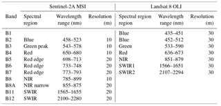
Table 1Spectral bands range and spatial resolution of Sentinel-2A MSI and Landsat 8 OLI sensors simulated in this study.
The full spectra of vegetation reflectance retrieved from the Fieldspec was used to model GPP, after excluding noisy values in the range 1350–1400 and 1800–1950 nm. Our P=1748 original explanatory variables are x350, …, x2299 where xλ represents the reflectance in the narrowband [λ, λ+1] (nm) and our response variable is the GPP (µmol m−2 s−1). A total number of 96 observations were available (4 treatments × 2 replicates × 3 blocks × 4 dates). Since we have 1748 explanatory variables and just 96 observations, hence a high level of redundancy in our data, the number of predictors were first reduced by grouping variables that belong to intervals of wavelengths at which all variables are highly correlated. A hierarchical cluster analysis was performed to reduce the number of predictors from P=1748 to p=25 groups of contiguous variables named “bands”. The basic idea is to aggregate contiguous and highly correlated individual 1 nm intervals of wavelength into broader wavelength bands. Two original predictors xλa, xλb are clustered together if their correlation coefficient r(xλa,xλb) is larger than 0.90. Bands correspond to the largest contiguous intervals at which all pairs of original predictors satisfy that condition. If a band groups all original predictors between λ1 and λ2, then it is represented by a new variable x[λ1,λ2], which is the arithmetic mean of the original variables xλ1, …, xλ2. The procedure is repeated to obtain all bands that partition the full x350, …, x2299 spectrum.
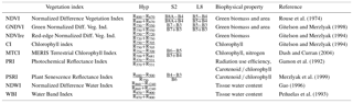
Table 2Selection of vegetation indices adopted in this study with their formulation using hyperspectral (Hyp) grouped bands, S2 or L8 simulated sensors, biophysical properties represented according to the literature and original bibliographic reference.
Reflectance values were also resampled to simulate bands of Sentinel-2A MSI (S2) and Landsat 8 OLI (L8). Since each band of S2 or L8 has a spectral response which is not perfectly uniform, we use the spectral response function of each sensor (Barsi et al., 2014; ESA, 2018) to weigh the contribution of each original predictor. As a result, for each sensor and band [λ1, λ2], we calculated the reflectance as a weighted mean of xλ1, …, xλ2, where the weights are given by the spectral response. The list of S2 and L8 bands used in this study is shown in Table 1.
Vegetation indices (VIs) (Table 2) were calculated from hyperspectral (Hyp), or simulated S2 and L8 sensors (Table 1). The selected VIs were retrieved from the literature based on their relation to biophysical properties of vegetation affecting GPP. Given that the goal of the analysis is to determine the set of VIs and/or bands that best model GPP, we apply a data analysis method that identifies the best subset of single variables. This is distinct from principal component analysis (PCA) where dimensionality reduction is achieved through replacing variables by their linear combinations, which still involve all the variables. We adopted linear regression (MLR) to model the relation between our explanatory variables (bands and VIs) and the response variable (GPP). Although the expressiveness of non-linear models (e.g. in the field of machine learning) is stronger than MLR, we believe that linear models provide a clearer interpretation of the relation between predictors and GPP, while offering enough flexibility by including variables in a high-dimensional representation space. Moreover, and as discussed below, linear models allow us to derive confidence intervals for our results, apply statistical tests to compare models at a given significance level, and they are less prone to overfitting than complex non-linear models.
Since the number of observations are only roughly twice as large as the number of new explanatory variables, we performed variable selection and excluded those that do not contribute significantly to the goodness-of-fit of our model. Although the dimensionality of the problem is very large, it can be solved efficiently by the LEAPS algorithm (Furnival and Wilson, 1974) available through the R package leaps (Lumley, 2009). Unlike alternative heuristic approaches (Cadima et al., 2004), LEAPS returns the optimal subset of predictors according to a given criteria. In our analysis, the criteria was the adjusted R2, so LEAPS returns the sub-model with the highest-adjusted R2 among all possible 2p sub-models, where p is the number of predictors.
A nested approach was adopted to formally test which model better explained GPP. A preliminary test showed that better results were obtained with exponential regressions and therefore ln GPP was adopted as the response variable in all analyses.
The general model was , where v is vegetation indices (VIs) or optical bands (B) from Hyp grouping procedure or from simulated S2 or L8 data. The subset of νj was selected by maximizing the adjusted R2 among all possible combinations of predictors. The LEAPS procedure returns an optimal model that we called L. However, L may include variables which contribute only marginally for the overall adjusted R2. To further reduce the dimensionality of the predictors, we test sub-models of L (obtained by backwards stepwise selection of predictors) against the LEAPS optimal model L. When sub-models of L were found not to be significantly worse than L at a significance level alpha=0.05, we then considered the most parsimonious of those sub-models as the optimal solution. A F test was used to perform those comparisons. The analysis was repeated separately for all vegetation indices (VIs) and bands (B) from Hyp, S2 or L8 data, obtaining an optimal model for each sensor. We performed an analysis of residuals for each selected model, which showed no evidence of violation of the linear model assumptions.
Besides determining the adjusted R2 for the optimal model from the full sample, we applied a bootstrap procedure (N=10 000 iterations) to estimate the distribution of the adjusted R2 in the whole population (Ohtani, 2000). This allowed us to estimate quantiles (25–75 %) for adjusted R2 and also compare the adjusted R2 distributions among models. In particular, it permits an estimation of the probability that the model A has a higher adjusted R2 than the alternative model B.
Two-step models were also used to investigate whether optical bands had the potential to improve models based only on vegetation indices (VIs). Toward that end, bands (B) were added to the optimal models obtained by the procedure described above denoted by Hyp-VIs, S2-VIs and L8-VIs (step 1). Using step 1 as the base model, we applied LEAPS to determine the subset of bands that maximized the overall adjusted R2. As before, we applied a F test (alpha=0.05) to possibly reduce the number of bands in the optimal model. As a result, we defined the optimal two-step models: Hyp-VIs+B, S2-VIs+B and L8-VIs+B. Finally, for Hyp, S2 and L8, we performed a F test to compare the one-step optimal model with the correspondent two-step optimal model. A low p value for this F test indicates that the two-step model is significantly better and means that bands, in addition to vegetation indices, contribute for an improved modelling of GPP.
3.1 Conditions during the experimental period
During the period of measurements, from 31 March to 3 June 2016, the average daily PAR and temperature increased progressively, ranging from 630 to 1000 µmol m−2 s−1 and from 9.6 to 17 ∘C, respectively (Fig. 1a). Soil water content (SWC) (Fig. 1b) showed fluctuations according to rainfall events, ranging from 0.05 to 0.2 m3 m−3. During the experimental period, rainfall was concentrated in the first half of April and at the beginning of May. Along the experimental period rainfall recorded was 195 mm, corresponding to the 33 % of the whole year.
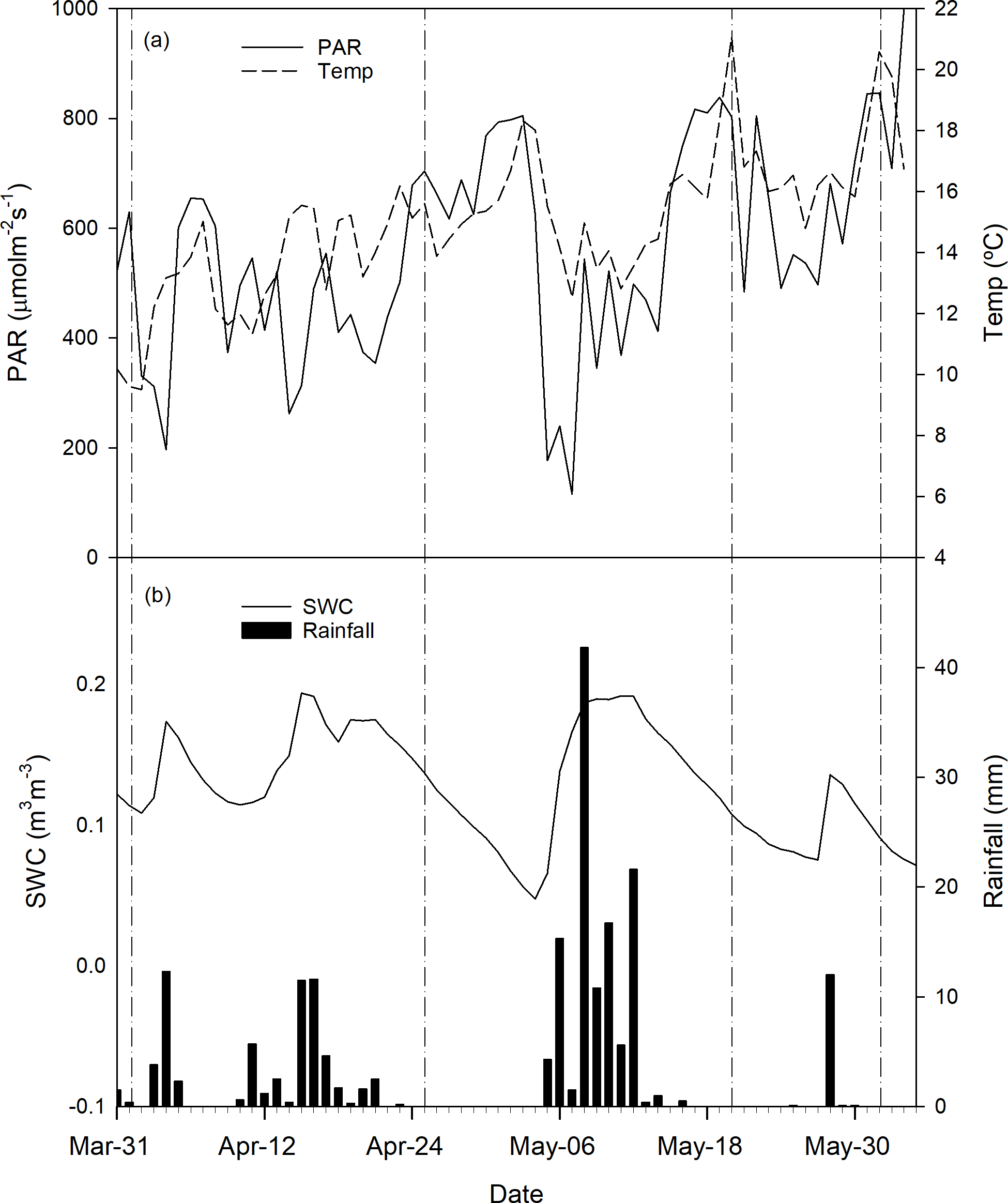
Figure 1Daily average PAR, temperature (a), soil water content for different treatments and total rainfall (b) recorded on the site during the experimental period. Dates of field measurements are indicated by vertical dashed-dotted lines.
3.2 The effect of fertilization on plant area index and functional groups proportion
From the beginning to the end of the study period, PAI increased on average 4-fold from 1 to 4 (Fig. 2a). In all treatments, the increase in PAI was completed by 20 May and no further increase was observed in the last measurement (3 June). On the contrary, at the beginning of the experiment, PAIgr (Fig. 2b) showed an increasing tendency similar to PAI, but from 20 May onwards, the tendency changed and a decrease was observed, corresponding to the onset of grassland senescence.
The fertilization treatments influenced both the PAI (P<0.000) and the PAIgr (P<0.000), being both significantly higher for treatments NPK and P than for treatment C (P<0.001). No differences were observed between C and N treatments (P>0.05). In both PAI and PAIgr the treatment P showed similar values to NPK, with the exception of the first measurement day (1 April). The grassland communities fertilized with NPK had a higher and earlier leaf area growth when compared to the other treatments.
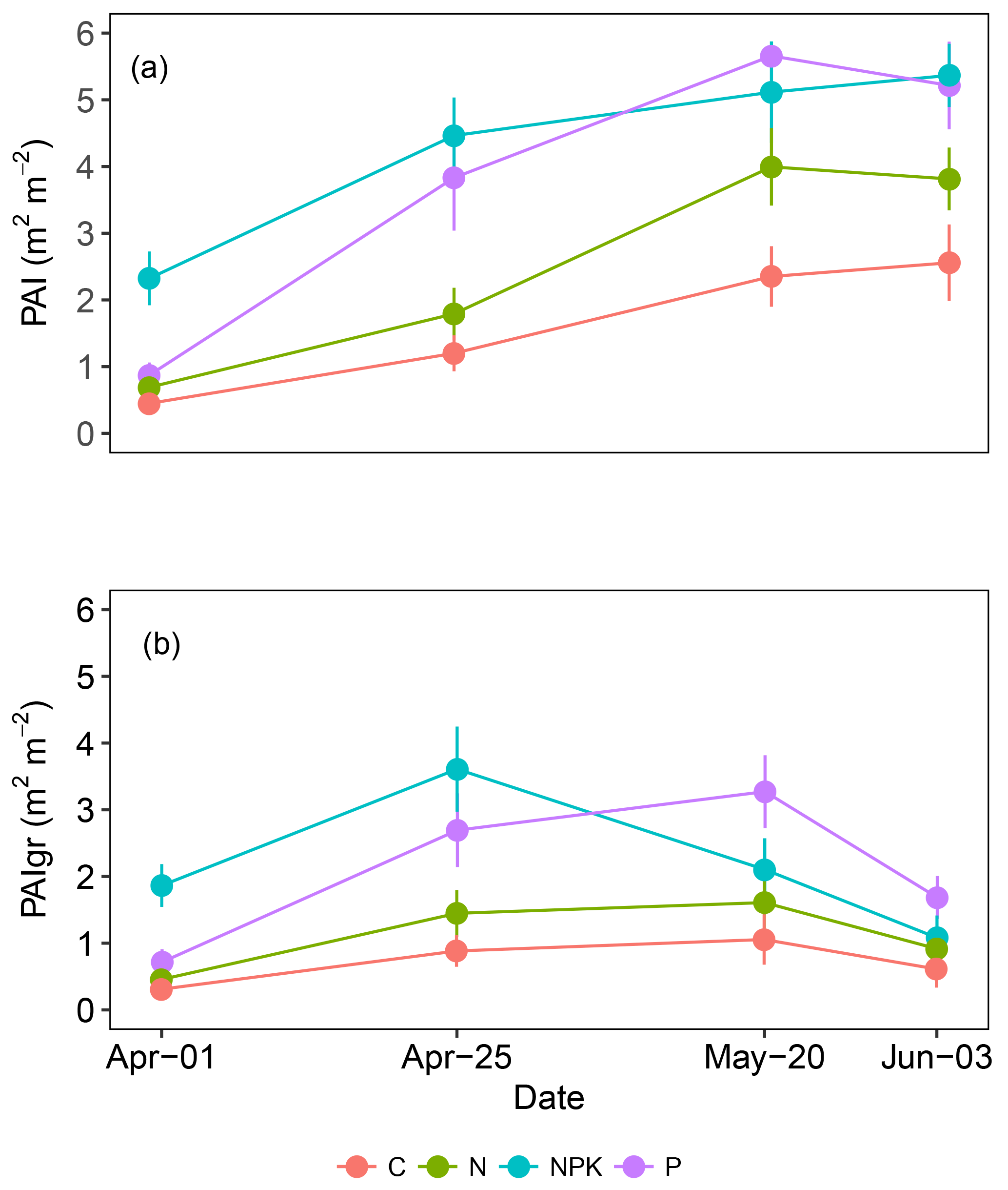
Figure 2Average green plant area index (PAI) and the green fraction of PAI (PAIgr) observed in grasslands subjected to different fertilization treatments (C, N, NPK or P). Each point is the average of six replicates. Vertical bars represent error bars.
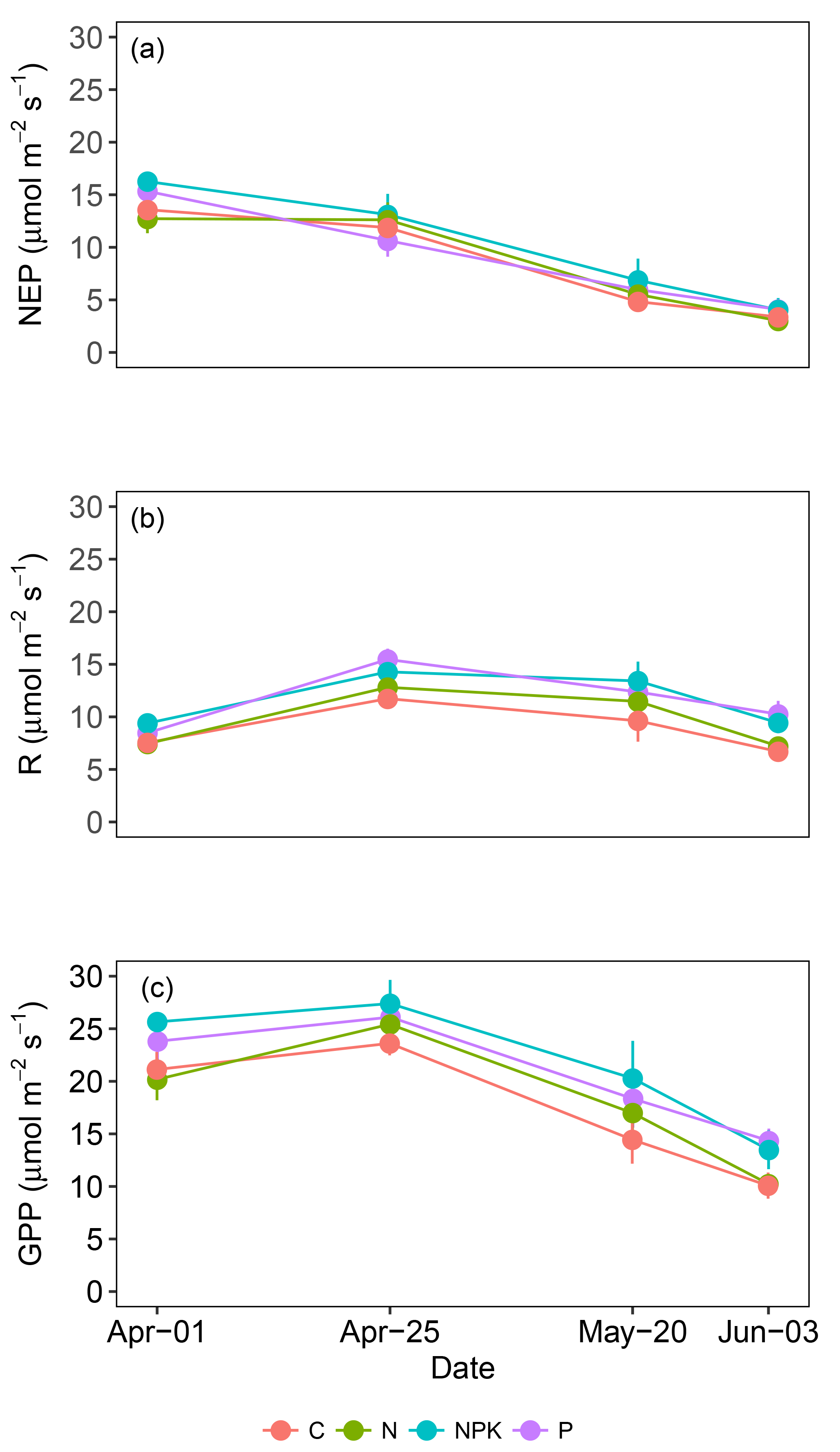
Figure 3Average net ecosystem productivity (NEP) (a), dark respiration (R) (b) and gross primary productivity (GPP) (c) measured in grasslands under different fertilization regimes (C, N, NPK and P). Each point is the average of 6 replicates. Vertical bars represent standard errors.
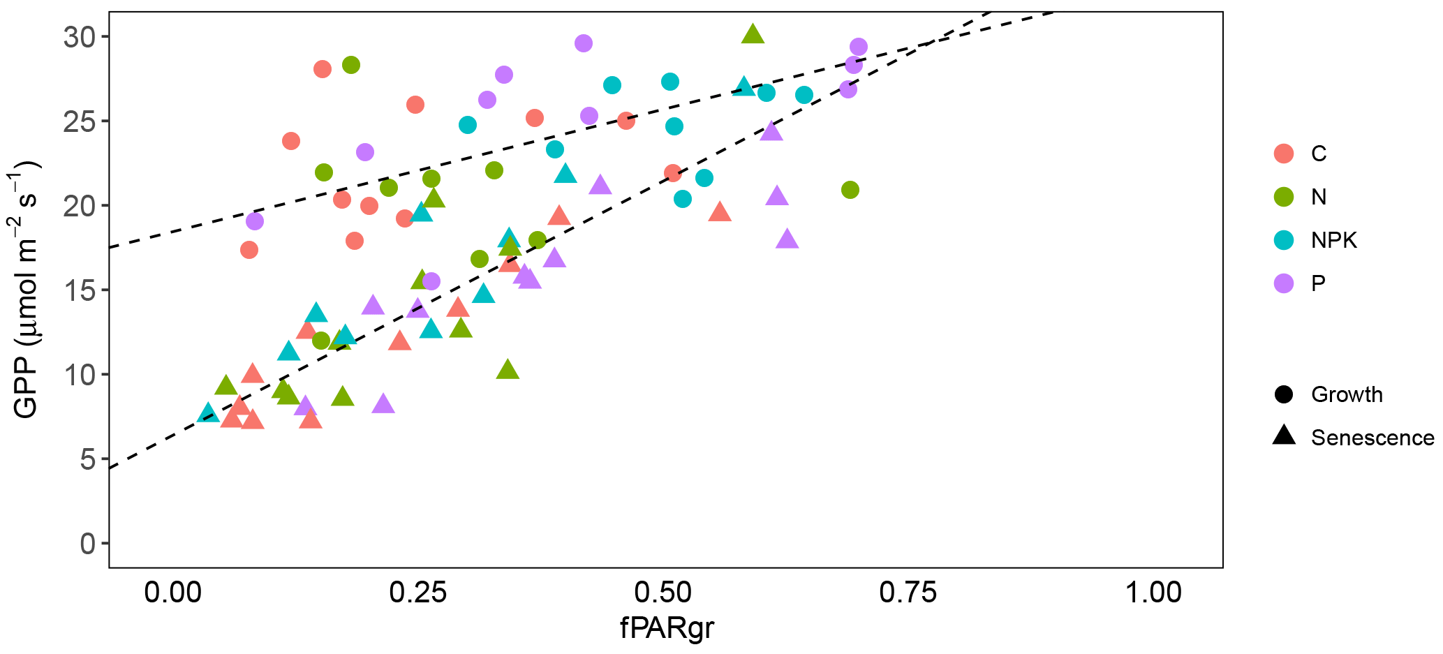
Figure 4Relationship between GPP and fPARgr observed in grassland subjected to different fertilization treatment (C, N, NPK and P). Measurements taken during the vegetation growth are indicated as circles (corresponding to measurement days 1 and 2), while those realized during the senescence period are indicated as triangles (measurement days 3 and 4). Linear regression lines were fitted separately to the two periods (, R2=0.39, P<0.001 and , R2=0.65, P<0.001, respectively for the growth and the senescence period).
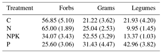
Plant species composition has been measured every year since 2012 (pre-treatment) under an ongoing long-term nutrient addition experiment on this grassland site. In line with results from that study (Carla Nogueira et al., personal communication, 2017), the fertilization treatments influenced the functional composition of grasslands (Table 3). In the NPK treatment the percentage of graminoids was higher than in any of the other treatments. P treatment showed a higher percentage of legumes and in the C and N treatments forbs were the dominant functional group.
Table 3Percentage of each plant functional type (Forbs, Graminoids and Legumes) in above-ground biomass of grasslands under different fertilization treatments (C, N, NPK and P). Values represent means of six replicates; standard errors are shown in parenthesis.
3.3 The effect of fertilization on GPP
The ability of grasslands to sequester atmospheric carbon dioxide was not affected by fertilization treatments. The NEP (Fig. 3a) and the GPP (Fig. 3c) did not reveal any statistically significant difference among treatments (P>0.05). On the contrary, the rate of respiration (Fig. 3b, R) was affected by the fertilization treatment (P<0.05), being on average higher for treatments NPK and P than C. CO2 gas exchanges were influenced by the grassland life cycle and marked trends were observed along the measurement period. NEP showed an average drop of 74 %, shifting from 14.47 to 3.67 µmol m−2 s−1, from 1 April (day 1) to 3 June (day 4) (P<0.000). This decrease in NEP rate was particularly evident from the second to the third measurement day, after the annual peak of grassland growth was achieved (Fig. 3a). R also showed differences along the experimental period (P<0.000) but the observed trend was different. R increased from the first to the second measurement day, from 8.22 to 13.65 µmol m−2 s−1 and then decreased toward the end of the experiment (Fig. 3b). GPP also changed significantly along the studied period (P<0.000), decreasing from 25.72 µmol m−2 s−1 on 25 April (day 2) to 12.12 µmol m−2 s−1 on 3 June (day 4). A linear relationship was observed between GPP and fPARgr (Fig. 4); however the slope of the regression line changed along the experimental period and marked differences were observed between the vegetation growth (day 1 and 2) and the senescence phase (day 3 and 4) (Fig. 4).
3.4 Vegetation reflectance
The reflectance of vegetation (Ref) varied on average between 0 and 0.4 (Fig. 5a). The cluster analysis created 25 bands (Fig. 5b) based on the Ref similarity of contiguous wavelengths (r>90 %). Bands were narrower in the visible region (350 to 750 nm) than in the NIR (750 to 1350 nm) and in the SWIR (1350 to 2300 nm) region. In particular, in the red-edge region, between 698 and 732 nm six different bands were identified, corresponding to a steep increase in reflectance observed in this region of the spectra.
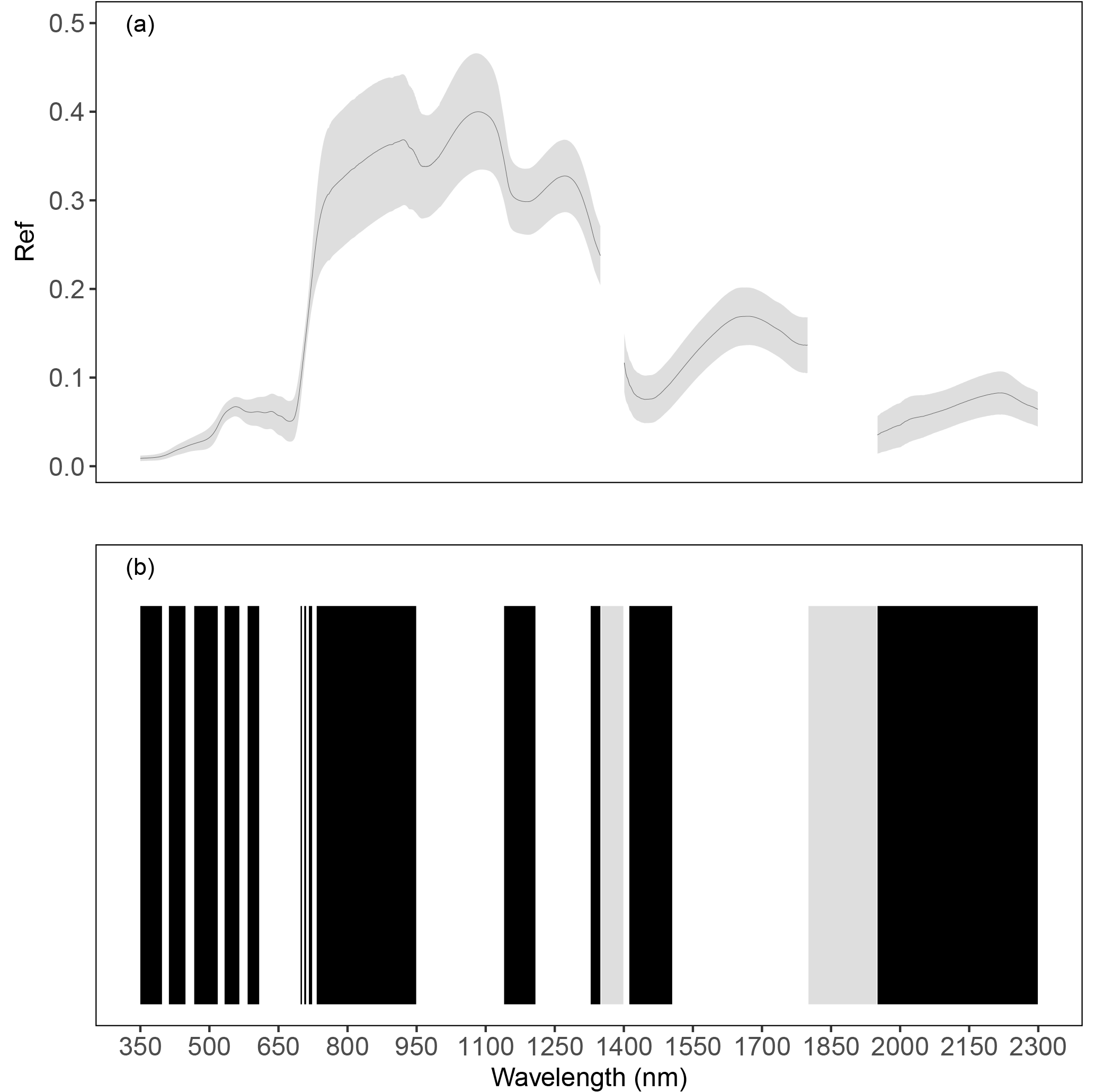
Figure 5Average reflectance values and standard deviation (grey ribbon) observed in herbaceous plots undergoing different fertilization treatments (a). The bottom picture (b) shows the bands obtained by grouping Ref for similarity ( %) of contiguous hyperspectral measurements with 1 nm resolution in the range 350–2300 nm; bands are alternately in black and white. Grey bars represent noisy regions of the spectrum not considered in the analysis.
3.5 Vegetation indices
When adopting wave bands obtained by cluster analysis (Fig. 5b) several vegetation indices were calculated (Table 2). The average values of the indices GNDVI, NDWI, PSRI and MTCI are shown in Fig. 5. Other indices are omitted from the figure for showing very similar trends to the ones represented (NDVI, NDVIre, WBI, CI) or not being significantly correlated with the response variable (PRI). All of them showed larger changes during the study period, particularly after 25 April (day 2), when the annual peak of growth was achieved.
The GNDVI (Fig. 6a) showed small changes among treatments and dates, with a significant drop of 20 % observed from 1 April to 3 June (P<0.000), and significant differences in the NPK and P treatments (P<0.001) compared to C but differences were not evident anymore on 3 June (day 4). The MTCI (Fig. 6b) showed a large drop that was particularly evident after 25 April (day 2). At 1 April (day 1), the effect of fertilization was evident in treatments NPK and P compared to C (P<0.001); however along the experimental period differences among treatments diminished and by 3 June (day 4) no differences among treatments were observed. The NDWI (Fig. 6c) showed a similar temporal trend with a marked decrease from 1 April to 3 June (P<0.001). Also, for MTCI, the NPK and P treatments always showed higher values than C (P<0.001), suggesting a positive impact of the higher nutrient availability on tissue water content. The PSRI had an opposite trend, showing on average a 3-fold increase from 1 April to 3 June (P<0.000) and a tendency to lower values in fertilized treatments compared to C (P<0.001 for NPK and P and P<0.01 for N).
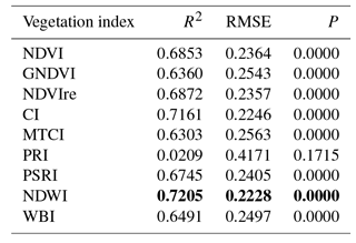
Significant regressions were established between GPP and all the vegetation indices considered (Table 4) with the exception of PRI. The NDWI was the index that explained the higher proportion of variability of GPP.
Table 4Linear regressions established between lnGPP and vegetation indices (VI) selected for this study (see Table 2). Best regression is shown in bold.
3.6 GPP estimates by multiple linear regression models
The LEAPS procedure selected VIs or bands as predictor variables that were retrieved from hyperspectral data (Hyp) or simulating Sentinel-2 MSI (S2) and Landsat 8 OLI (L8) sensors.
The Hyp and S2 models adopting only VIs as predictor variables (Hyp-VIs and S2-VIs) performed similarly, with a considerable overlap of adjusted R2 (Table 5). On the contrary, the L8-VIs model showed a lower performance (lower adjusted R2) than Hyp-VIs and S2-VI models (Table 5). Bootstrap results allowed us to conclude, at a confidence level of 90 %, that Hyp-VIs have higher adjusted R2 than L8-VIs.
Table 5Best selection of linear models for a GPP estimate according to the general equation: , where v is vegetation indices (VIs) or optical bands (B). Bands and vegetation indices are obtained from hyperspectral measurements grouped in clusters with 90 % similarity (Hyp) or resampled for simulating Sentinel-2 MSI (S2) and Landsat 8 OLI (L8) sensors. Formulation of vegetation indices is shown in Table 2. The order of the variables (most important first) reflects their importance in the model. The quantiles 25 % and 75 % of the adj R2 are obtained from a bootstrap with 10 000 iterations. The two-step models add a selection of bands to the variables (VIs) selected at step 1. A low p value indicates that the step 2 model, including VIs and bands (step 2) is significantly better the corresponding step 1 model.
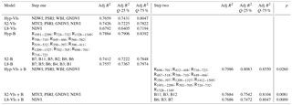
The selection of VIs in the Hyp-VIs and S2-VIs models exhibited a similar spectral pattern. Both models included PSRI and GNDVI. On the contrary, NDVI, the most frequently adopted index as green leaf area proxy was not included in the Hyp-VIs model but only in the S2-VIs. Two of the indices included in the Hyp model are related to water balance (WBI) and water tissue content (NDWI). The S2 model also includes MTCI, which represents chlorophyll a and N.
Models including only bands (-B) showed similar performances to respective models employing vegetation indices (-VIs). Only in the case of L8, where just one vegetation index (NDVI) was available, bands (L8-B) led to better modelling of GPP than vegetation indices (L8-VIs). Similar spectral patterns were also observed in the selection of bands for GPP estimate for all sensors (Hyp, S2, L8). A common pattern is the inclusion of bands in the SWIR region that are strongly represented in the Hyp-B (R1951−2299, R1209−1327, R1328−1349), S2-B (B11) and L8-B (B6 and B7) models. The red-edge region of the spectra was also largely represented in the Hyp-B (R724−732, R706−710, R702−705, R698−701, R716−723) and S2-B (B5, B6 and B7), underlining the importance of this region for vegetation reflectance.
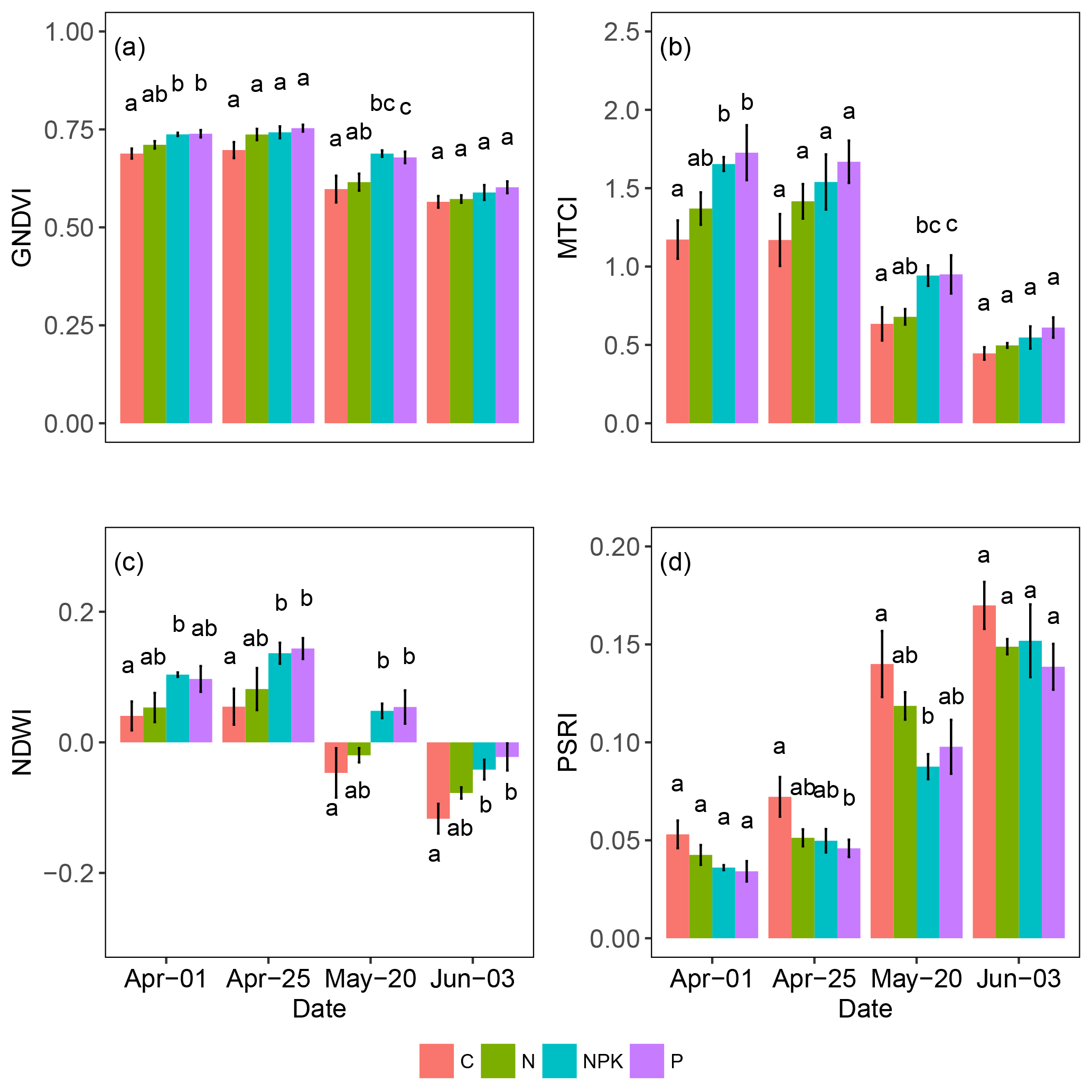
Figure 6Average values of several vegetation indices retrieved from reflectance measurements of herbaceous plots undergoing different fertilization treatments. Vertical bars represent standard errors. Different letters indicate significant differences among treatments within the same date (P<0.05).
The LEAPS two-step procedure allowed us to identify bands with the potential to improve the VI-based models, identifying regions of the spectra that are generally not adopted in vegetation indices. For both S2 and L8 the two-step model (VIs+B) significantly increased (P<0.010) the performance of the model, while for Hyp the difference between Hyp-VIs and Hyp-VIs+B model, in spite of still being significant, is less marked (P<0.05). The bootstrap procedure indicated that the probability of the Hyp-VIs+B being significantly better is 83 % when compared to S2-VIs+B and 81 % when compared to L8-VIs+B. On the contrary, the S2-VIs+B and L8-VIs+B models do not differ significantly. In all VIs+B models, bands in the SWIR region were included. The second region of the spectra that was more represented in the Hyp-B and Hyp-VIs+B model was the red edge.
4.1 The impact of fertilization treatment
The fertilization treatment influenced the growth rate and the composition of the herbaceous plots more than carbon sequestration. In line with a 5-year ongoing study at the same grassland site, the fertilization treatment resulted in differences in proportions of above-ground biomass and functional groups for NPK and P treatments compared to C, while the single addition of N had no effect.
An earlier growth response was also observed in the NPK treatment. The higher percentage of graminoid species with on average higher growth rates compared to most forb species (Ansquer et al., 2009; Craine et al., 2001; Westoby et al., 2002) could explain early differences in PAI and PAIgr in this treatment. As leaf area is usually positively related to GPP (e.g. Aires et al., 2008b; Xu and Baldocchi, 2004), it would be expected that higher PAIgr in NPK treatments would induce increased GPP. However, confounding factors such as increased water demand associated with higher growth rates might have downscaled differences between treatments (e.g. Weisser et al., 2017).
The relationship GPP-fPARgr showed some differences along the experiment. The slope of the regression line was considerably lower during the vegetative growth than during the senescence period (Fig. 4), revealing the occurrence of marked changes in the effective LUE along the growth life cycle and confirming previous results (Nestola et al., 2016; Pérez-Priego et al., 2015a).
While the fertilization treatment had no impact on NEP or GPP, a higher R rate was observed at the measurement day 4 (3 June) in the NPK and P treatments. Differences can be ascribed to the higher PAI, and precipitation at the end of May, which must have stimulated soil respiration (Jarvis et al., 2007; Reichstein et al., 2003).
4.2 Best VIs for GPP estimation
The LEAPS procedure selected several indices as significant predictor variables for GPP in the Hyp-VIs and S2-VIs model (Table 5). The vegetation indices selected in the Hyp-VIs and S2-VIs models are known to represent different properties of vegetation, specifically: the green fraction of the leaf area (GNDVI and NDVI), the chlorophyll a and N concentration (MTCI), the ratio carotenoids ∕ chlorophyll (PSRI) and the tissue water content (NDWI, WBI). Each of these traits has a major role in GPP.
Among the vegetation indices selected in the multiple linear models, both the Hyp-VIs and the S2-VIs included PSRI (Merzlyak et al., 1999), which is generally applied to detect the occurrence of vegetation senescence. PSRI is able to capture changes in the carotenoids ∕ chlorophyll ratio occuring during vegetation senescence since chlorophyll declines more rapidly than carotenoids (Merzlyak et al., 1999). In this study, PSRI increased in all treatments after 25 April, when the maximum peak of growth (Fig. 2b) was achieved and close to the onset of canopy drying out. Another index known to be related to the carotenoids ∕ chlorophyll ratio, the PRI (Filella et al., 2009), showed no correlation with GPP in our study. These results are in contrast with previous studies (Pérez-Priego et al., 2015a). However, a low performance of PRI in representing the carotenoids ∕ chlorophyll ratio has been already observed in semi-arid grasslands (Vicca et al., 2016). In crops, a good agreement between PRI and pigment pools was observed at leaf level (Gitelson et al., 2017a) but not at stand level (Gitelson et al., 2017b). Differences in the last two studies were ascribed to changes in canopy structure (e.g. changes in leaf inclination angle) over the growing season.
The Hyp model also gave evidence of the importance of changes in canopy water content, as both NDWI (Gao, 1996) and WBI (Peñuelas et al., 1997) were included in the model. Considering changes observed in NDWI along the experiment and the good correlation observed between NDWI or WBI and GPP it is reasonable to assume that GPP is largely affected by the progressive senescence of vegetation (Balzarolo et al., 2015; Vescovo et al., 2012). In a previous study, Vicca et al. (2016) found that NDWI was able to estimate GPP in semi-arid grasslands better than other indices, allowing the effect of drought to be distinguished.
Other indices that are sensitive to changes in chlorophyll a concentration, MTCI (Dash and Curran, 2004) and GNDVI (Gitelson and Merzlyak, 1998) were also included in the model. The fertilization treatment resulted in an increase in MTCI during the first stage of the experiment in the NPK and P treatments, followed by a decrease observed in all treatments as the season progressed toward the end of the annual growth cycle. A similar trend was observed in a study by Pérez-Priego et al. (2015a) in which Mediterranean grasslands were subjected to fertilization with N or NP. The primary role of chlorophyll in photosynthesis is well known and justifies the positive relationship observed between GPP and MTCI. However, in the present study, no differences were observed in GPP among fertilized and non-fertilized treatments, suggesting that the expected increase in photosynthesis due to the increase in chlorophyll and nitrogen was constrained by other environmental and physiological factors.
Notably NDVI, the most frequently applied index in GPP estimates by LUE models (Yuan et al., 2014) was not selected in the Hyp-VIs model and showed a poorer coefficient of determination than other indices (e.g. NDWI). NDVI is expected to reflect changes in green leaf area, being generally linearly related to the fraction of photosynthetically absorbed radiation (Myneni and Williams, 1994). However, previous studies reported a saturation of NDVI and consequent lack of linearity in the regression in highly productive vegetation communities (Gianelle et al., 2009; Vescovo et al., 2012), such as grasslands, and sometimes other indices showed a better performance. For example, in grasslands subjected to water and nutrient stress, the NDVI green index (GNDVI), which adopts a green band instead of the red band of NDVI and is hence more sensitive to chlorophyll a concentration (Gitelson et al., 1996), showed a better performance than NDVI as proxy of leaf area (Cristiano et al., 2010; Gianelle et al., 2009). Also, in this study, the GNDVI explained a larger proportion of GPP variance than NDVI in the Hyp-VIs and S2-VIs models being selected in both and before NDVI in the S2-VIs model.
The indices selected by the LEAPS (i.e. NDVI, GNDVI, NDWI, MTCI, PSRI and WBI) also showed a highly significant relationship with GPP (Table 4) in simple regressions, explaining 63 % to 72 % of the variability observed. The functional convergence (Ollinger, 2011) of different traits participating in the photosynthetic process may have hampered results observed in the regression for each single vegetation index, showing a high degree of correlation for most of them (Table 4). However, the selection of several VIs, representative of different structural and functional traits in the multiple linear models and the lower performance observed in the L8 model, including solely the NDVI index, clearly indicate the importance of considering the contribution of different traits with different temporal dynamics to capture GPP temporal changes in models integrating vegetation indices.
4.3 Are spectral bands better GPP estimators than VIs?
Our results suggest a marginal improvement in GPP estimates obtained by adopting bands (Hyp-B, S2-B, Table 5) instead of vegetation indices (Hyp-VIs, S2-VIs, Table 5). However, a large impact was observed in the case of the L8-VIs+B model when compared with the L8-VIs model which included only NDVI (Table 5).
These results confirm previous studies comparing the explanatory power of VIs and bands in grasslands (Balzarolo et al., 2015; Matthes et al., 2015), also evidencing the importance of the selection of the proper spectral range and suggesting that the selection of the proper band is equally important to the mathematical formulation of vegetation indices for the explanatory power of spectral retrievals. In our study, the adopted approach assured a high correlation among wavelengths within a band maximizing their representativeness.
However, it cannot be disregarded that VIs offer, in comparison with spectral bands, the advantage of being more robust in representing vegetation features, since differences resulting from background reflectance, sun-sensor geometry and atmospheric effects are mitigated by normalization of spectral values (Glenn et al., 2008).
Our results also evidenced the importance of the SWIR region of the spectra, as bands in this region were selected in all one- and two-step models, which is rarely adopted in vegetation indices with few exceptions. The SWIR region is known to correlate with canopy water content (Casas et al., 2014). Studies investigating the potential of spectral bands to estimate canopy chlorophyll content and green fAPAR found that the SWIR region was strongly positively correlated with them in grasslands (Sakowska et al., 2016) and also GPP in a semi-arid savanna (Tagesson et al., 2015).
Bands in the red-edge region were also largely represented in the Hyp-B, S2-B and in the Hyp-VIs+B models. The red edge corresponds to the steep increase in reflectance at the boundary between the red region, where chlorophyll is absorbed, and the leaf scattering at the NIR region. Red-edge bands were successfully employed to estimate chlorophyll content in maize (Zhang and Zhou, 2017) and LAI in crops (Kira et al., 2017). For these reasons they were integrated into numerous VIs, such as MTCI and PSRI, which were also applied in this study. This explains the lack of red-edge bands in the second step of the S2 model (S2-VIs+B) but strong representation in the S2-B.
4.4 Satellite sensors as estimators of GPP
Differences in the selection of the vegetation indices among sensors had apparently no effect on the performance of the S2-VIs and Hyp-VIs models (Table 5), while the limited number of available vegetation indices for the L8 resulted in a lower performance of the model. Our results show that S2 and L8 spectral signatures are equally suitable for assessing GPP.
GPP estimates obtained by simulating S2 and L8 sensors showed similar performances in the -B and -VIs+B models, while when only VIs were adopted, the S2 model had clearly a better performance than L8. These results suggest a need for testing new vegetation indices adopting L8 bands. In agreement with our results, other studies comparing linear additive models showed a similar ability in estimating canopy cover and LAI adopting the S2 or L8 sensors (Korhonen et al., 2017).
An important difference between the S2 and L8 availability of wavebands is the lack of reflectance values in the red-edge region for L8, which limited the possibility of computing VIs, such as MTCI and PSRI (Korhonen et al., 2017). However, the limitation imposed by the lack of bands in the red-edge region, had apparently more importance for the -VIs model, while differences in the performance of the model between S2 and L8 decreased for -B and VIs+B models.
In this study, the S2 and L8 data comparison was based only on the simulation of the respective bands and did not take into consideration other factors that possibly affected the spectral response of sensors such as sun-sensor viewing geometry (Tagesson et al., 2015). Nonetheless, in a recent study (Korhonen et al., 2017), the comparisons of satellite data from the two platforms showed no differences between S2 and L8 reflectance values in the NIR, SWIR1 and SWIR 2 bands. In other regions of the spectra, such as the green and blue bands, reflectance values were considerably smaller in the S2 than in the L8 but still proportional, suggesting that comparisons between S2 and L8 simulated bands can largely be representative of the actual differences obtained by the two remote platforms.
Our results confirm the importance of performing hyperspectral measurements. Indeed, inferential bootstrap results show that for the whole population, and with a probability of 80 %, the Hyp-VIs+B model is superior to the corresponding S2 and L8 models. The high resolution and the wide range of wave bands makes hyperspectral sensors unique in identifying regions of the spectra that are of high interest for representing different vegetation properties (Porcar-Castell et al., 2015).
In agreement with previous studies (Pérez-Priego et al., 2015a; Rossini et al., 2012; Vicca et al., 2016), our results clearly indicate the need to integrate spectral information into GPP models, representing both structural and functional traits of vegetation along the whole grasslands life cycle. Specifically, water content (NDWI), chlorophyll (MTCI, GNDVI) and the ratio of chlorophyll to carotenoids (PSRI) were indicated as best predictor variables for GPP estimates. Altogether these vegetation indices describe the loss of photosynthetic pigments and efficiency and drying out of vegetation, and when considered together they considerably improved GPP estimates in comparison with models that only adopt NDVI.
Our study also confirms the importance of hyperspectral in situ measurements for an exploratory analysis of the relationship between biophysical and optical properties of vegetation, providing a wide spectral range and high resolution of spectral retrievals.
The hyperspectral reflectance values, together with the two-step procedure adopted for the selection of predictor variables, also gave evidence to critical regions of the spectra, which were not included in the initial selection of vegetation indices but revealed their usefulness in estimating GPP. For example, the LEAPS two-step procedure evidenced which bands could significantly improve a -VIs model (step 1), identifying the red edge and SWIR regions of the spectra to be of major importance for improving GPP estimates. This information can be critical in the development of new spectral indices and sensors.
Our results also evidenced the potential of S2 and L8 sensor in assessing GPP, since models obtained by simulating bands from the two sensors showed similar performances. The possibility of using remote-sensing information for monitoring and modelling vegetation at a suitable spatial resolution, such as in the S2 and L8 sensors, allows for attempted vegetation monitoring and modelling in a cost-effective way, in support of sustainable agriculture management practices.
All data in the paper are available online at https://doi.org/10.1594/PANGAEA.892837 (Cerasoli et al., 2018).
SC designed the experiment and performed field measurements together with JF. MC developed the variable selection code. CN and MdCC set up the experimental plots. SC prepared the manuscript with contributions from all the authors.
The authors declare that they have no conflict of interest.
This work was funded by Fundação para a Ciência e a Tecnologia,
Ministry of Science and Education, through the project MEDSPEC, Monitoring
gross primary productivity in Mediterranean oak woodlands through remote
sensing and biophysical modelling (PTDC/AAG-MAA/3699/2014), and the research
activities of the Forest Research Centre (PEsst-OE/AGR/UI0239/2011).
Sofia Cerasoli is post-doc fellow (BPD/SFRH/78998/2011), Carla Nogueira is
the recipient of a PhD grant (SFRH/BD/88650/2012). Authors wish to thank
Georg Wohlfarth for a critical reading of the manuscript and Joaquim Mendes,
Madalena Silva, Lurdes Marçal, Alicia Horta and Paula Pais for technical
help in the field and laboratory. Authors are also grateful to FLAD/NSF for
funding (A1/Proj 124/12) and to the Companhia das Lezírias for providing
access to the grassland site and permission to undertake
research.
Edited by: Christopher A.
Williams
Reviewed by: two anonymous referees
Aires, L. M., Pio, C. A., and Pereira, J. S.: The effect of drought on energy and water vapour exchange above a mediterranean C3 ∕ C4 grassland in Southern Portugal, Agr. Forest Meteorol., 148, 565–579, https://doi.org/10.1016/j.agrformet.2007.11.001, 2008a.
Aires, L. M., Pio, C. A., and Pereira, J. S.: Carbon dioxide exchange above a Mediterranean C3 ∕ C4 grassland during two climatologically contrasting years, Glob. Change Biol., 14, 539–555, https://doi.org/10.1111/j.1365-2486.2007.01507.x, 2008b.
Ansquer, P., Duru, M., Theau, J. P., and Cruz, P.: Convergence in plant traits between species within grassland communities simplifies their monitoring, Ecol. Indic., 9, 1020–1029, https://doi.org/10.1016/J.ECOLIND.2008.12.002, 2009.
Asner, G. P., Nepstad, D., Cardinot, G., and Ray, D.: Drought stress and carbon uptake in an Amazon forest measured with spaceborne imaging spectroscopy, P. Natl. Acad. Sci. USA, 101, 6039–6044, https://doi.org/10.1073/pnas.0400168101, 2004.
Balzarolo, M., Vescovo, L., Hammerle, A., Gianelle, D., Papale, D., Tomelleri, E., and Wohlfahrt, G.: On the relationship between ecosystem-scale hyperspectral reflectance and CO2 exchange in European mountain grasslands, Biogeosciences, 12, 3089–3108, https://doi.org/10.5194/bg-12-3089-2015, 2015.
Barsi, J., Lee, K., Kvaran, G., Markham, B., and Pedelty, J.: The Spectral Response of the Landsat-8 Operational Land Imager, Remote Sens., 6, 10232–10251, https://doi.org/10.3390/rs61010232, 2014.
Bates, D., Mächler, M., Bolker, B., and Walker, S.: Fitting Linear Mixed-Effects Models using lme4, J. Stat. Softw., 67, 1–48, https://doi.org/10.18637/jss.v067.i01, 2014.
Beer, C., Reichstein, M., Tomelleri, E., Ciais, P., Jung, M., Carvalhais, N., Rödenbeck, C., Arain, M. A., Baldocchi, D., Bonan, G. B., Bondeau, A., Cescatti, A., Lasslop, G., Lindroth, A., Lomas, M., Luyssaert, S., Margolis, H., Oleson, K. W., Roupsard, O., Veenendaal, E., Viovy, N., Williams, C., Woodward, F. I., and Papale, D.: Terrestrial gross carbon dioxide uptake: global distribution and covariation with climate, Science, 329, 834–838, https://doi.org/10.1126/science.1184984, 2010.
Borer, E. T., Grace, J. B., Harpole, W. S., MacDougall, A. S., and Seabloom, E. W.: A decade of insights into grassland ecosystem responses to global environmental change, Nat. Ecol. Evol., 1, 0118, https://doi.org/10.1038/s41559-017-0118, 2017.
Bugalho, M. N. and Abreu, J. M.: The multifunctional role of grasslands, in: Sustainable Mediterranean Grasslands and their Multifunctions, Vol. 79, Option Méditerraneénes, edited by: Porqueddu, C. and Tavares de Sousa, M. M., CIHEAM/FAO/ENMP/SPPF, Zaragoza, 25–30, 2008.
Cadima, J., Cerdeira, J., and Minhoto, M.: Computational aspects of algorithms for variable selection in the context of principal components, Comput. Stat. Data An., 47, 225–236, https://doi.org/10.1016/j.csda.2003.11.001, 2004.
Casas, A., Riaño, D., Ustin, S. L., Dennison, P., and Salas, J.: Estimation of water-related biochemical and biophysical vegetation properties using multitemporal airborne hyperspectral data and its comparison to MODIS spectral response, Remote Sens. Environ., 148, 28–41, https://doi.org/10.1016/j.rse.2014.03.011, 2014.
Cerasoli, S., Campagnolo, M., Faria, J., Nogueira, C., and Caldeira, M. C.: Hyperspectral reflectance, gas exchange and meteorological conditions in grassland plots undergoing different fertilization regimes in Central Portugal from March to June 2016, PANGAEA, https://doi.org/10.1594/PANGAEA.892837, 2018.
Ceulemans, T., Stevens, C. J., Duchateau, L., Jacquemyn, H., Gowing, D. J. G., Merckx, R., Wallace, H., van Rooijen, N., Goethem, T., Bobbink, R., Dorland, E., Gaudnik, C., Alard, D., Corcket, E., Muller, S., Dise, N. B., Dupré, C., Diekmann, M., and Honnay, O.: Soil phosphorus constrains biodiversity across European grasslands, Glob. Change Biol., 20, 3814–3822, https://doi.org/10.1111/gcb.12650, 2014.
Cheng, Y.-B., Zhang, Q., Lyapustin, A. I., Wang, Y., and Middleton, E. M.: Impacts of light use efficiency and fPAR parameterization on gross primary production modeling, Agr. Forest Meteorol., 189–190, 187–197, https://doi.org/10.1016/j.agrformet.2014.01.006, 2014.
Costa, A. C., Santos, J. A., and Pinto, J. G.: Climate change scenarios for precipitation extremes in Portugal, Theor. Appl. Climatol., 108, 217–234, https://doi.org/10.1007/s00704-011-0528-3, 2012.
Craine, J. M., Froehle, J., Tilman, D. G., Wedin, D. A., and Chapin, III, F. S.: The relationships among root and leaf traits of 76 grassland species and relative abundance along fertility and disturbance gradients, Oikos, 93, 274–285, https://doi.org/10.1034/j.1600-0706.2001.930210.x, 2001.
Cristiano, P. M., Posse, G., Di Bella, C. M., and Jaimes, F. R.: Uncertainties in fPAR estimation of grass canopies under different stress situations and differences in architecture, Int. J. Remote Sens., 31, 4095–4109, https://doi.org/10.1080/01431160903229192, 2010.
Dash, J. and Curran, P. J.: The MERIS terrestrial chlorophyll index, Int. J. Remote Sens., 25, 5403–5413, https://doi.org/10.1080/0143116042000274015, 2004.
Díaz-Villa, M. D., Marañón, T., Arroyo, J., and Garrido, B.: Soil seed bank and floristic diversity in a forest-grassland mosaic in southern Spain, J. Veg. Sci., 14, 701–709, https://doi.org/10.1111/j.1654-1103.2003.tb02202.x, 2003.
Drusch, M., Del Bello, U., Carlier, S., Colin, O., Fernandez, V., Gascon, F., Hoersch, B., Isola, C., Laberinti, P., Martimort, P., Meygret, A., Spoto, F., Sy, O., Marchese, F., and Bargellini, P.: Sentinel-2: ESA's Optical High-Resolution Mission for GMES Operational Services, Remote Sens. Environ., 120, 25–36, https://doi.org/10.1016/j.rse.2011.11.026, 2012.
ESA: Sentinel-2 Data Quality Report Issue 24 (February 2018) – Sentinel-2 MSI Document Library – User Guides – Sentinel Online, available at: https://earth.esa.int/web/sentinel/user-guides/sentinel-2-msi/document-library/-/asset_publisher/Wk0TKajiISaR/content/ (last access: 25 January 2018), 2018.
Fensholt, R., Sandholt, I., and Rasmussen, M. S.: Evaluation of MODIS LAI, fAPAR and the relation between fAPAR and NDVI in a semi-arid environment using in situ measurements, Remote Sens. Environ., 91, 490–507, https://doi.org/10.1016/j.rse.2004.04.009, 2004.
Filella, I., Peñuelas, J., Llorens, L., and Estiarte, M.: Reflectance assessment of seasonal and annual changes in biomass and CO2 uptake of a Mediterranean shrubland submitted to experimental warming and drought, Remote Sens. Environ., 90, 308–318, https://doi.org/10.1016/J.RSE.2004.01.010, 2004.
Filella, I., Porcar-Castell, A., Munné-Bosch, S., Bäck, J., Garbulsky, M. F., and Peñuelas, J.: PRI assessment of long-term changes in carotenoids/chlorophyll ratio and short-term changes in de-epoxidation state of the xanthophyll cycle, Int. J. Remote Sens., 30, 4443–4455, https://doi.org/10.1080/01431160802575661, 2009.
Filippa, G., Cremonese, E., Migliavacca, M., Galvagno, M., Forkel, M., Wingate, L., Tomelleri, E., Morra di Cella, U., and Richardson, A. D.: Phenopix: A R package for image-based vegetation phenology, Agr. Forest Meteorol., 220, 141–150, https://doi.org/10.1016/j.agrformet.2016.01.006, 2016.
Furnival, G. M. and Wilson, R. W.: Regressions by Leaps and Bounds, Technometrics, 16, 499–511, https://doi.org/10.1080/00401706.1974.10489231, 1974.
Galloway, J. N., Dentener, F. J., Capone, D. G., Boyer, E. W., Howarth, R. W., Seitzinger, S. P., Asner, G. P., Cleveland, C. C., Green, P. A., Holland, E. A., Karl, D. M., Michaels, A. F., Porter, J. H., Townsend, A. R., and Vosmarty, C. J.: Nitrogen Cycles: Past, Present, and Future, Biogeochemistry, 70, 153–226, https://doi.org/10.1007/s10533-004-0370-0, 2004.
Gamon, J. A.: Reviews and Syntheses: optical sampling of the flux tower footprint, Biogeosciences, 12, 4509–4523, https://doi.org/10.5194/bg-12-4509-2015, 2015.
Gamon, J. A., Penuelas, J., and Field, C. B.: A narrow-wave band spectral index that tracks diurnal changes in photosynthetic efficiency, Remote Sens. Environ., 41, 35–44, 1992.
Gamon, J. A., Serrano, L., and Surfus, J. S.: The photochemical reflectance index: an optical indicator of photosynthetic radiation use efficiency across species, functional types, and nutrient levels, Oecologia, 112, 492–501, https://doi.org/10.1007/s004420050337, 1997.
Gao, B.: NDWI – A normalized difference water index for remote sensing of vegetation liquid water from space, Remote Sens. Environ., 58, 257–266, https://doi.org/10.1016/S0034-4257(96)00067-3, 1996.
Garbulsky, M. F., Peñuelas, J., Gamon, J., Inoue, Y., and Filella, I.: The photochemical reflectance index (PRI) and the remote sensing of leaf, canopy and ecosystem radiation use efficienciesA review and meta-analysis, Remote Sens. Environ., 115, 281–297, https://doi.org/10.1016/j.rse.2010.08.023, 2011.
Gianelle, D., Vescovo, L., Marcolla, B., Manca, G., and Cescatti, A.: Ecosystem carbon fluxes and canopy spectral reflectance of a mountain meadow, Int. J. Remote Sens., 30, 435–449, https://doi.org/10.1080/01431160802314855, 2009.
Gitelson, A. and Merzlyak, M. N.: Spectral reflectance changes associated with autumn senescence of Aesculus-Hippocastanum L. and Acer-Platanoides L leaves – spectral features and relation to chlorophyll estimation, J. Plant Physiol., 143, 286–292, 1994.
Gitelson, A. A. and Merzlyak, M. N.: Remote sensing of chlorophyll concentration in higher plant leaves, Adv. Space Res., 22, 689–692, https://doi.org/10.1016/S0273-1177(97)01133-2, 1998.
Gitelson, A. A., Kaufman, Y. J., and Merzlyak, M. N.: Use of a green channel in remote sensing of global vegetation from EOS-MODIS, Remote Sens. Environ., 58, 289–298, https://doi.org/10.1016/S0034-4257(96)00072-7, 1996.
Gitelson, A. A., Gamon, J. A., and Solovchenko, A.: Multiple drivers of seasonal change in PRI: Implications for photosynthesis 1. Leaf level, Remote Sens. Environ., 191, 110–116, https://doi.org/10.1016/j.rse.2016.12.014, 2017a.
Gitelson, A. A., Gamon, J. A., and Solovchenko, A.: Multiple drivers of seasonal change in PRI: Implications for photosynthesis 2. Stand level, Remote Sens. Environ., 190, 198–206, https://doi.org/10.1016/J.RSE.2016.12.015, 2017b.
Glenn, E., Huete, A., Nagler, P., and Nelson, S.: Relationship Between Remotely-sensed Vegetation Indices, Canopy Attributes and Plant Physiological Processes: What Vegetation Indices Can and Cannot Tell Us About the Landscape, Sensors, 8, 2136–2160, https://doi.org/10.3390/s8042136, 2008.
Gower, S. T., Kucharik, C. J., and Norman, J. M.: Direct and Indirect Estimation of Leaf Area Index, fAPAR, and Net Primary Production of Terrestrial Ecosystems, Remote Sens. Environ., 70, 29–51, https://doi.org/10.1016/S0034-4257(99)00056-5, 1999.
Harpole, W. S., Potts, D. L., and Suding, K. N.: Ecosystem responses to water and nitrogen amendment in a California grassland, Glob. Change Biol., 13, 2341–2348, https://doi.org/10.1111/j.1365-2486.2007.01447.x, 2007.
Hothorn, T., Bretz, F., and Westfall, P.: Simultaneous Inference in General Parametric Models, Biometrical J., 50, 346–363, https://doi.org/10.1002/bimj.200810425, 2008.
INMG: O clima de Portugal. Normais climatológicas da região Ribatejo e Oeste correspondentes a 1951–1980, Instituto Nacional de Meteorologia e Geofisica, Lisboa, Portugal, 1991.
Jarvis, P., Rey, A., Petsikos, C., Wingate, L., Rayment, M., Pereira, J., Banza, J., David, J., Miglietta, F., Borghetti, M., Manca, G., and Valentini, R.: Drying and wetting of Mediterranean soils stimulates decomposition and carbon dioxide emission: the “Birch effect”, Tree Physiol., 27, 929–940, https://doi.org/10.1093/treephys/27.7.929, 2007.
Joel, G., Gamon, J. A., and Field, C. B.: Production efficiency in sunflower: The role of water and nitrogen stress, Remote Sens. Environ., 62, 176–188, https://doi.org/10.1016/s0034-4257(97)00093-x, 1997.
Jones, H. G.: Plants amd microclimate: A quantitative approach to Environmental Plant Physiology, 2nd Edn., Cambridge University Press, Cambridge, 1992.
Jongen, M., Pereira, J. S., Aires, L. M., and Pio, C. A.: The effects of drought and timing of precipitation on the inter-annual variation in ecosystem-atmosphere exchange in a Mediterranean grassland, Agr. Forest Meteorol., 151, 595–606, https://doi.org/10.1016/j.agrformet.2011.01.008, 2011.
Jongen, M., Lecomte, X., Unger, S., Fangueiro, D., and Pereira, J. S.: Precipitation variability does not affect soil respiration and nitrogen dynamics in the understorey of a Mediterranean oak woodland, Plant Soil, 372, 235–251, https://doi.org/10.1007/s11104-013-1728-7, 2013a.
Jongen, M., Unger, S., Fangueiro, D., Cerasoli, S., Silva, J. M. N., and Pereira, J. S.: Resilience of montado understorey to experimental precipitation variability fails under severe natural drought, Agr. Ecosyst. Environ., 178, 18–30, 2013b.
Kira, O., Nguy-Robertson, A. L., Arkebauer, T. J., Linker, R., and Gitelson, A. A.: Toward generic models for green LAI estimation in maize and soybean: Satellite observations, Remote Sens., 9, 318, https://doi.org/10.3390/rs9040318, 2017.
Korhonen, L., Hadi, Packalen, P., and Rautiainen, M.: Comparison of Sentinel-2 and Landsat-8 in the estimation of boreal forest canopy cover and leaf area index, Remote Sens. Environ., 195, 259–274, https://doi.org/10.1016/j.rse.2017.03.021, 2017.
Kovats, R. S., Valentini, R., Bouwer, L. M., Georgopoulou, E., Jacob, D., Martin, E., Rounsevell, M., and Soussana, J. F.: Europe, in: Climate Change 2014: Impacts, Adaptation, and Vulnerability. Part B: Regional Aspects. Contribution of Working Group II to the Fifth Assessment Report of the Intergovernmental Panel on Climate Change, 1267–1326, Cambridge University Press, Cambridge, UK and New York, NY, USA, 2014.
Loveland, T. R. and Irons, J. R.: Landsat-8: The plans, the reality, and the legacy, Remote Sens. Environ., 185, 1–6, https://doi.org/10.1016/j.rse.2016.07.033, 2016.
Lumley, T.: Thomas Lumley using Fortran code by Alan Miller (2009). Leaps: regression subset selection, R package version 2.9, 2009.
Matthes, J. H., Knox, S. H., Sturtevant, C., Sonnentag, O., Verfaillie, J., and Baldocchi, D.: Predicting landscape-scale CO2 flux at a pasture and rice paddy with long-term hyperspectral canopy reflectance measurements, Biogeosciences, 12, 4577–4594, https://doi.org/10.5194/bg-12-4577-2015, 2015.
Merzlyak, M. N., Gitelson, A. A., Chivkunova, O. B., and Rakitin, V. Y.: Non-destructive optical detection of pigment changes during leaf senescence and fruit ripening, Physiol. Plant., 106, 135–141, https://doi.org/10.1034/j.1399-3054.1999.106119.x, 1999.
Monteith, J. L.: Solar Radiation and Productivity in Tropical Ecosystems, J. Appl. Ecol., 9, 747–766, https://doi.org/10.2307/2401901, 1972.
Monteith, J. L.: Climate and efficiency of crop production in Britain, Philos. T. Roy. Soc. B, 281, 277–294, 1977.
Moreno, A., Maselli, F., Gilabert, M. A., Chiesi, M., Martinez, B., and Seufert, G.: Assessment of MODIS imagery to track light-use efficiency in a water-limited Mediterranean pine forest, Remote Sens. Environ., 123, 359–367, https://doi.org/10.1016/j.rse.2012.04.003, 2012.
Myneni, R. B. and Williams, D. L.: On the relationship between FAPAR and NDVI, Remote Sens. Environ., 49, 200–211, 1994.
Nestola, E., Calfapietra, C., Emmerton, C. A., Wong, C. Y. S., Thayer, D. R., and Gamon, J. A.: Monitoring grassland seasonal carbon dynamics, by integrating MODIS NDVI, proximal optical sampling, and eddy covariance measurements, Remote Sens., 8, 260, https://doi.org/10.3390/rs8030260, 2016.
Ohtani, K.: Bootstrapping R2 and adjusted R2 in regression analysis, Econ. Model., 17, 473–483, https://doi.org/10.1016/S0264-9993(99)00034-6, 2000.
Ollinger, S. V.: Sources of variability in canopy reflectance and the convergent properties of plants, New Phytol., 189, 375–394, https://doi.org/10.1111/j.1469-8137.2010.03536.x, 2011.
Peñuelas, J., Filella, I., Biel, C., Serrano, L., and Savé, R.: The reflectance at the 950–970 nm region as an indicator of plant water status, Int. J. Remote Sens., 14, 1887–1905, https://doi.org/10.1080/01431169308954010, 1993.
Peñuelas, J., Filella, I., and Gamon, J. A.: Assessment of photosynthetic radiation-use efficiency with spectral reflectance, New Phytol., 131, 291–296, https://doi.org/10.1111/j.1469-8137.1995.tb03064.x, 1995.
Peñuelas, J., Pinol, J., Ogaya, R., and Filella, I.: Estimation of plant water concentration by the reflectance Water Index WI (R900/R970), Int. J. Remote Sens., 18, 2869–2875, https://doi.org/10.1080/014311697217396, 1997.
Peñuelas, J., Poulter, B., Sardans, J., Ciais, P., van der Velde, M., Bopp, L., Boucher, O., Godderis, Y., Hinsinger, P., Llusia, J., Nardin, E., Vicca, S., Obersteiner, M., and Janssens, I. A.: Human-induced nitrogen–phosphorus imbalances alter natural and managed ecosystems across the globe, Nat. Commun., 4, 2934, https://doi.org/10.1038/ncomms3934, 2013.
Pérez-Priego, O., Guan, J., Rossini, M., Fava, F., Wutzler, T., Moreno, G., Carvalhais, N., Carrara, A., Kolle, O., Julitta, T., Schrumpf, M., Reichstein, M., and Migliavacca, M.: Sun-induced chlorophyll fluorescence and photochemical reflectance index improve remote-sensing gross primary production estimates under varying nutrient availability in a typical Mediterranean savanna ecosystem, Biogeosciences, 12, 6351–6367, https://doi.org/10.5194/bg-12-6351-2015, 2015a.
Pérez-Priego, O., López-Ballesteros, A., Sánchez-Cañete, E., Serrano-Ortiz, P., Kutzbach, L., Domingo, F., Eugster, W., and Kowalski, A.: Analysing uncertainties in the calculation of fluxes using whole-plant chambers: random and systematic errors, Plant Soil, 393, 229–244, https://doi.org/10.1007/s11104-015-2481-x, 2015b.
Porcar-Castell, A., Garcia-Plazaola, J. I., Nichol, C. J., Kolari, P., Olascoaga, B., Kuusinen, N., Fernandez-Marin, B., Pulkkinen, M., Juurola, E., and Nikinmaa, E.: Physiology of the seasonal relationship between the photochemical reflectance index and photosynthetic light use efficiency, Oecologia, 170, 313–323, https://doi.org/10.1007/s00442-012-2317-9, 2012.
Porcar-Castell, A., Mac Arthur, A., Rossini, M., Eklundh, L., Pacheco-Labrador, J., Anderson, K., Balzarolo, M., Martín, M. P., Jin, H., Tomelleri, E., Cerasoli, S., Sakowska, K., Hueni, A., Julitta, T., Nichol, C. J., and Vescovo, L.: EUROSPEC: at the interface between remote-sensing and ecosystem CO2 flux measurements in Europe, Biogeosciences, 12, 6103–6124, https://doi.org/10.5194/bg-12-6103-2015, 2015.
R Core Team: R: A language and environment for statistical computing, R Foundation for Statistical Computing, Vienna, Austria, available at: https://www.R-project.org/ (last access: 7 August 2018), 2017.
Reichstein, M., Rey, A., Freibauer, A., Tenhunen, J., Valentini, R., Banza, J., Casals, P., Cheng, Y., Grünzweig, J. M., Irvine, J., Joffre, R., Law, B. E., Loustau, D., Miglietta, F., Oechel, W., Ourcival, J.-M., Pereira, J. S., Peressotti, A., Ponti, F., Qi, Y., Rambal, S., Rayment, M., Romanya, J., Rossi, F., Tedeschi, V., Tirone, G., Xu, M., and Yakir, D.: Modeling temporal and large-scale spatial variability of soil respiration from soil water availability, temperature and vegetation productivity indices, Global Biogeochem. Cy., 17, 1104, https://doi.org/10.1029/2003GB002035, 2003.
Rossini, M., Cogliati, S., Meroni, M., Migliavacca, M., Galvagno, M., Busetto, L., Cremonese, E., Julitta, T., Siniscalco, C., Morra di Cella, U., and Colombo, R.: Remote sensing-based estimation of gross primary production in a subalpine grassland, Biogeosciences, 9, 2565–2584, https://doi.org/10.5194/bg-9-2565-2012, 2012.
Rouse, J. W., Haas, R. H., Schell, J. A., and Deering, D. W.: Monitoring vegetation systems in the great plains with ERTS, in: Third ERTS Symposium, Vol. 1, SP-351, 309–317, NASA, Washington, DC, USA, 1974.
Sakowska, K., Vescovo, L., Marcolla, B., Juszczak, R., Olejnik, J., and Gianelle, D.: Monitoring of carbon dioxide fluxes in a subalpine grassland ecosystem of the Italian Alps using a multispectral sensor, Biogeosciences, 11, 4695–4712, https://doi.org/10.5194/bg-11-4695-2014, 2014.
Sakowska, K., Juszczak, R., and Gianelle, D.: Remote Sensing of Grassland Biophysical Parameters in the Context of the Sentinel-2 Satellite Mission, J. Sensors, 2016, 1–16, https://doi.org/10.1155/2016/4612809, 2016.
Sala, O. E.: Global Biodiversity Scenarios for the Year 2100, Science, 287, 1770–1774, https://doi.org/10.1126/science.287.5459.1770 2000.
Schenk, H. J. and Jackson, R. B.: Rooting depths, lateral root spreads and below-ground/above-ground allometries of plants in water-limited ecosystems, J. Ecol., 90, 480–494, https://doi.org/10.1046/j.1365-2745.2002.00682.x, 2002.
Schimel, D., Pavlick, R., Fisher, J. B., Asner, G. P., Saatchi, S., Townsend, P., Miller, C., Frankenberg, C., Hibbard, K., and Cox, P.: Observing terrestrial ecosystems and the carbon cycle from space, Glob. Change Biol., 21, 1762–1776, https://doi.org/10.1111/gcb.12822, 2015.
Seabloom, E. W., Borer, E. T., Buckley, Y., Cleland, E. E., Davies, K., Firn, J., Harpole, W. S., Hautier, Y., Lind, E., MacDougall, A., Orrock, J. L., Prober, S. M., Adler, P., Alberti, J., Michael Anderson, T., Bakker, J. D., Biederman, L. A., Blumenthal, D., Brown, C. S., Brudvig, L. A., Caldeira, M., Chu, C., Crawley, M. J., Daleo, P., Damschen, E. I., D'Antonio, C. M., DeCrappeo, N. M., Dickman, C. R., Du, G., Fay, P. A., Frater, P., Gruner, D. S., Hagenah, N., Hector, A., Helm, A., Hillebrand, H., Hofmockel, K. S., Humphries, H. C., Iribarne, O., Jin, V. L., Kay, A., Kirkman, K. P., Klein, J. A., Knops, J. M. H., La Pierre, K. J., Ladwig, L. M., Lambrinos, J. G., Leakey, A. D. B., Li, Q., Li, W., McCulley, R., Melbourne, B., Mitchell, C. E., Moore, J. L., Morgan, J., Mortensen, B., O'Halloran, L. R., Pärtel, M., Pascual, J., Pyke, D. A., Risch, A. C., Salguero-Gómez, R., Sankaran, M., Schuetz, M., Simonsen, A., Smith, M., Stevens, C., Sullivan, L., Wardle, G. M., Wolkovich, E. M., Wragg, P. D., Wright, J., and Yang, L.: Predicting invasion in grassland ecosystems: is exotic dominance the real embarrassment of richness?, Glob. Change Biol., 19, 3677–3687, https://doi.org/10.1111/gcb.12370, 2013.
Tagesson, T., Fensholt, R., Huber, S., Horion, S., Guiro, I., Ehammer, A., and Ardö, J.: Deriving seasonal dynamics in ecosystem properties of semi-arid savanna grasslands from in situ-based hyperspectral reflectance, Biogeosciences, 12, 4621–4635, https://doi.org/10.5194/bg-12-4621-2015, 2015.
Thomas, H.: Senescence, ageing and death of the whole plant, New Phytol., 197, 696–711, https://doi.org/10.1111/nph.12047, 2013.
Vescovo, L., Wohlfahrt, G., Balzarolo, M., Pilloni, S., Sottocornola, M., Rodeghiero, M., and Gianelle, D.: New spectral vegetation indices based on the near-infrared shoulder wavelengths for remote detection of grassland phytomass, Int. J. Remote Sens., 33, 2178–2195, https://doi.org/10.1080/01431161.2011.607195, 2012.
Vicca, S., Balzarolo, M., Filella, I., Granier, A., Herbst, M., Knohl, A., Longdoz, B., Mund, M., Nagy, Z., Pintér, K., Rambal, S., Verbesselt, J., Verger, A., Zeileis, A., Zhang, C., and Peñuelas, J.: Remotely-sensed detection of effects of extreme droughts on gross primary production, Sci. Rep.-UK, 6, 28269, https://doi.org/10.1038/srep28269, 2016.
Viña, A. and Gitelson, A. A.: New developments in the remote estimation of the fraction of absorbed photosynthetically active radiation in crops, Geophys. Res. Lett., 32, L17403, https://doi.org/10.1029/2005GL023647, 2005.
Weisser, W. W., Roscher, C., Meyer, S. T., Ebeling, A., Luo, G., Allan, E., Beßler, H., Barnard, R. L., Buchmann, N., Buscot, F., Engels, C., Fischer, C., Fischer, M., Gessler, A., Gleixner, G., Halle, S., Hildebrandt, A., Hillebrand, H., de Kroon, H., Lange, M., Leimer, S., Le Roux, X., Milcu, A., Mommer, L., Niklaus, P. A., Oelmann, Y., Proulx, R., Roy, J., Scherber, C., Scherer-Lorenzen, M., Scheu, S., Tscharntke, T., Wachendorf, M., Wagg, C., Weigelt, A., Wilcke, W., Wirth, C., Schulze, E.-D., Schmid, B., and Eisenhauer, N.: Biodiversity effects on ecosystem functioning in a 15-year grassland experiment: Patterns, mechanisms, and open questions, Basic Appl. Ecol., 23, 1–73, https://doi.org/10.1016/j.baae.2017.06.002, 2017.
Westoby, M., Falster, D. S., Moles, A. T., Vesk, P. A., and Wright, I. J.: Plant Ecological Strategies: Some Leading Dimensions of Variation Between Species, Annu. Rev. Ecol. Syst., 33, 125–159, https://doi.org/10.1146/annurev.ecolsys.33.010802.150452, 2002.
WRB: IUSS Working Group: World reference base for soil resources 2006, 2nd Edn., World Soil Resources Reports No. 103, FAO, Rome, Italy, 2006.
Xu, L. and Baldocchi, D. D.: Seasonal variation in carbon dioxide exchange over a Mediterranean annual grassland in California, Agr. Forest Meteorol., 123, 79–96, https://doi.org/10.1016/j.agrformet.2003.10.004, 2004.
Yuan, W., Cai, W., Xia, J., Chen, J., Liu, S., Dong, W., Merbold, L., Law, B., Arain, A., Beringer, J., Bernhofer, C., Black, A., Blanken, P. D., Cescatti, A., Chen, Y., Francois, L., Gianelle, D., Janssens, I. A., Jung, M., Kato, T., Kiely, G., Liu, D., Marcolla, B., Montagnani, L., Raschi, A., Roupsard, O., Varlagin, A., and Wohlfahrt, G.: Global comparison of light use efficiency models for simulating terrestrial vegetation gross primary production based on the LaThuile database, Agr. Forest Meteorol., 192–193, 108–120, https://doi.org/10.1016/j.agrformet.2014.03.007, 2014.
Zhang, F. and Zhou, G.: Deriving a light use efficiency estimation algorithm using in situ hyperspectral and eddy covariance measurements for a maize canopy in Northeast China, Ecol. Evol., 7, 4735–4744, https://doi.org/10.1002/ece3.3051, 2017.