the Creative Commons Attribution 4.0 License.
the Creative Commons Attribution 4.0 License.
 | 19 Sep 2018
Greenhouse gas emissions from boreal inland waters unchanged after forest harvesting
Marcus Klaus
Erik Geibrink
Anders Jonsson
Ann-Kristin Bergström
David Bastviken
Hjalmar Laudon
Jonatan Klaminder
Jan Karlsson
Forestry practices often result in an increased export of carbon and nitrogen to downstream aquatic systems. Although these losses affect the greenhouse gas (GHG) budget of managed forests, it is unknown if they modify GHG emissions of recipient aquatic systems. To assess this question, air–water fluxes of carbon dioxide (CO2), methane (CH4) and nitrous oxide (N2O) were quantified for humic lakes and their inlet streams in four boreal catchments using a before-after control-impact experiment. Two catchments were treated with forest clear-cuts followed by site preparation (18 % and 44 % of the catchment area). GHG fluxes and hydrological and physicochemical water characteristics were measured at multiple locations in lakes and streams at high temporal resolution throughout the summer season over a 4-year period. Both lakes and streams evaded all GHGs. The treatment did not significantly change GHG fluxes in streams or lakes within 3 years after the treatment, despite significant increases of CO2 and CH4 concentrations in hillslope groundwater. Our results highlight that GHGs leaching from forest clear-cuts may be buffered in the riparian zone–stream continuum, likely acting as effective biogeochemical processors and wind shelters to prevent additional GHG evasion via downstream inland waters. These findings are representative of low productive forests located in relatively flat landscapes where forestry practices cause only a limited initial impact on catchment hydrology and biogeochemistry.
- Article
(7191 KB) - Full-text XML
-
Supplement
(1417 KB) - BibTeX
- EndNote


Land use activities have greatly enhanced inputs of carbon (C) and nitrogen (N) from terrestrial or atmospheric sources to the aquatic environment, reducing the terrestrial C sink function and aggravating global climate change (Dawson and Smith, 2007; Regnier et al., 2013; Vitousek et al., 1997). The terrestrial C sink is largely determined by forest ecosystems which contribute to a net uptake of greenhouse gases (GHG) from the atmosphere (Goodale et al., 2002; Myneni et al., 2001). This net uptake can be further increased by well-informed forest harvesting strategies (Kaipainen et al., 2004; Liski et al., 2001). Hence, forest management is a widely used instrument to fulfill GHG budget commitments under the Kyoto Protocol (IGBP Terrestrial Carbon Working Group, 1998). Yet, mitigation measures neglect to consider that a significant part of terrestrial C and N taken up by forests is exported to aquatic systems (Battin et al., 2009; Öquist et al., 2014; Sponseller et al., 2016). These exports are sensitive to logging activity (Nieminen, 2004; Schelker et al., 2012; Lamontagne et al., 2000), and a large proportion is processed in inland waters and emitted back to the atmosphere as GHGs such as carbon dioxide (CO2), methane (CH4) and nitrous oxide (N2O) (Cole et al., 2007; Seitzinger and Kroeze, 1998). Revealing potential changes in the GHG budget of the aquatic environment downstream forest clear-cuts is therefore crucial to evaluate the overall potential of forestry to mitigate climate warming.
Forestry effects on aquatic GHG emissions are largely unknown and difficult to predict due to multiple processes involved. In boreal headwaters, stream and lake CO2 and CH4 originate largely from soils (Bogard and del Giorgio, 2016; Hotchkiss et al., 2015; Rasilo et al., 2017). These soil-derived inputs typically increase after forest clear-cutting because of increased soil respiration (Bond-Lamberty et al., 2004; Kowalski et al., 2003) and discharge (Andréassian, 2004; Martin et al., 2000). Forest clear-cutting often also increases dissolved organic carbon (DOC) export to streams and lakes (Schelker et al., 2012; Nieminen, 2004; France et al., 2000), where it stimulates respiration and reduces light penetration, lake primary production, and net CO2 uptake (Ask et al., 2012; Lapierre et al., 2013). Therefore, any elevated terrestrial C inputs due to forest clear-cutting may further increase net heterotrophy and CO2 emissions (Ouellet et al., 2012) or stimulate methanogenic bacterial activity in lakes (Huttunen et al., 2003). Forest clear-cuts also often enhance nutrient exports, with less pronounced changes for phosphorous but large increases for N, especially for nitrate (Nieminen, 2004; Palviainen et al., 2014; Schelker et al., 2016). Nitrate leakage affect GHG cycling in boreal inland waters, yet predictions on the direction of net effects are difficult. Nitrate inputs may suppress (Liikanen et al., 2003) or stimulate (Bogard et al., 2014) CH4 production, enhance CH4 oxidation (Deutzmann et al., 2014), and promote denitrification and N2O emissions (McCrackin and Elser, 2010; Seitzinger and Nixon, 1985). Nitrate inputs to N-limited boreal aquatic systems stimulate phytoplankton production and thereby enhance CO2 uptake and oxygen (O2) production (Bergström and Jansson, 2006). Increases in DOC would, however, consume O2 (Houser et al., 2003) and changes in O2 concentrations have been identified to influence the balance between methanogenesis and methanotrophy (Bastviken et al., 2008) as well as nitrification and denitrification (Mengis et al., 1997). Removal of riparian vegetation may increase littoral light availability and water temperature (Steedman et al., 2001; Moore, 2005), with potential effects on net CO2 and CH4 production (Wik et al., 2014; Yvon-Durocher et al., 2012, 2014). Forest clear-cuts could also increase wind exposure (Tanentzap et al., 2008; Xenopoulos and Schindler, 2001) and thus result in increased gas transfer velocities as indicated by the wind based relationships found in lakes (Cole and Caraco, 1998). Likewise, enhanced discharge may affect turbulence and gas transfer velocities in streams (Raymond et al., 2012). Clear-cut effects on hydrology and biogeochemistry can be further amplified by site preparation, i.e., the trenching of soils before replanting (Schelker et al., 2012; Palviainen et al., 2014).
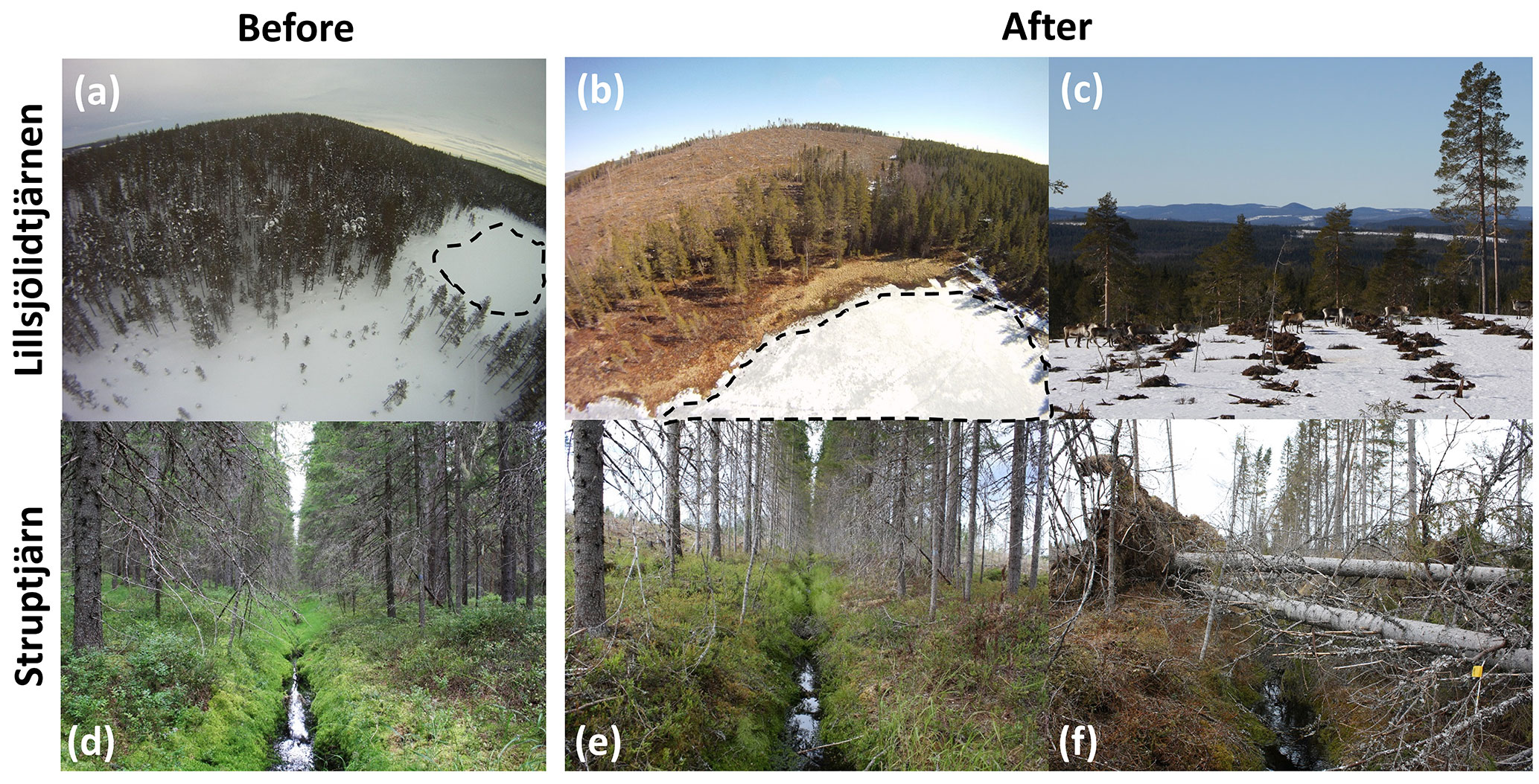
Figure 1Forest–stream–lake continuum before (a, d) and after (b, c, e, f) clear-cutting in the ice-covered lake Lillsjölidtjärnen (a–c) and the inlet of Struptjärn (d–f). The dashed line shows the contours of Lillsjölidtjärnen. Note the soil trenches (snow-free patches) after site preparation (c) and the storm damage of the riparian buffer vegetation (f).
Even though spatial surveys indicate that changes in vegetation (Maberly et al., 2013; Urabe et al., 2011), forest fires (Marchand et al., 2009), and forestry activities (Ouellet et al., 2012) affect the GHG balance of inland waters, mechanistic evidence from whole-catchment forest manipulation experiments is lacking. Here, the impact of forest clear-cuts and site preparation on the summer season's (June–September) means of air–water CO2, CH4, and N2O fluxes was experimentally assessed for streams and lakes in four boreal headwater catchments. A whole-catchment manipulation experiment was performed using a before-after control-impact (BACI) design. Two “impact” catchments received a forest clear-cut and site preparation following 1 year of pretreatment sampling. Two “control” catchments were left untreated throughout the whole study period of 4 years. We hypothesized an increase in aquatic CO2, CH4, and N2O emissions in response to forest clear-cuts and site preparation.
2.1 Study sites
Sampling was carried out during June–September 2012–2015 in four headwater lakes and three lake inlet streams (one lake lacks an inlet stream) in the catchments (220–400 m a.s.l.) of Övre Björntjärn, Stortjärn, Struptjärn and Lillsjölidtjärnen, northern Sweden (Table 1, Fig. 1). During the experimental period, mean annual temperature in the region was 1–3 ∘C higher than the long-term average (1960–1990) of 1.0 ∘C, while annual precipitation was close to the long-term average of 500–600 mm in all years except for 2012, which had 800 mm (http://www.smhi.se/klimatdata/meteorologi, last access: 14 September 2018). In the study catchments, mean summer air temperatures and precipitation sums (June–September) varied between 11.1 ∘C and 342 mm in 2012 and 12.8 ∘C and 245 mm in 2014, respectively (Table S1 in the Supplement). Catchment soils were typically well drained and characterized by podzol with a 10–15 cm thick organic layer developed on locally derived glacial till and granitic bedrock. The catchments were mainly (>85 %) covered by managed coniferous forest (Picea abies, Pinus sylvestris) with scattered birch trees (Betula sp.) and minerogenic oligotrophic mires (<15 %). Site quality class was rather low with timber productivities of 2–3 m3 ha−1 yr−1 (SLU, 2005). The catchments were drained by a hand dug ditch network established in the early 20th century to improve the forest's productivity. The riparian zone was about 2–6 m wide and characterized by organic rich peat soils. The regional hydrology is characterized by pronounced snowmelt episodes in April and May, summer and winter low-flow periods, and autumn storms with enhanced precipitation. Drainage channels all culminate in single lake inlets with average specific discharges of 1.0, 1.4, and 1.5 mm d−1 in Struptjärn, Lillsjölidtjärnen, and Övre Björntjärn in June–September 2012. The study lakes were shallow, small, humic, and dimictic with a seasonal mixed layer depth of 0.5–2 m during summer stratification lasting from late May to mid-September. Lake ice was present from late October to mid-May during the study period.
Table 1Morphological and physicochemical characteristics of the lakes and streams of the experimental catchments. Temporally variable parameters are given as mean values of the pretreatment period (June–September 2012). Abbreviations: a420 is the spectral absorbance at 420 nm, DOC is dissolved organic carbon concentration, TP is total phosphorous concentration, and TN is total nitrogen concentration.
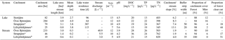
* Clear-cut.
2.2 Forest clear-cutting and site preparation procedure
Forest clear-cutting was carried out on snow-covered (∼ 60 cm) frozen soil in February 2013 in the catchments of Struptjärn and Lillsjölidtjärnen by national or private forest companies according to common practice methods of whole-tree harvesting where about 30 % of tops, twigs, and needles were left on-site (Fig. 1). The forests cut were coniferous forests with an age of about 90–120 years. In early November 2014, clear-cuts were site-prepared by disc trenching, a common soil scarification method to improve planting conditions (Fig. 1c). Clear-cut areas were defined by the forest companies, 14 and 11 ha in size, and corresponded to 18 % and 44 % of total lake watershed areas, respectively (Table 1). Clear-cuts covered 40 % and 60 % of the stream reaches of the inlets of Struptjärn and Lillsjölidtjärnen. Along the inlet stream of Lillsjölidtjärnen, 10–70 m wide stream buffer strips were left and remained intact throughout the study period. Buffer strips along the inlet stream of Struptjärn were <10 m (Fig. 1e) and damaged by a wind throw event in winter 2014/15, where 70 % of trees within the buffer strip fell along half of the clear-cut affected reach, causing a bank collapse and soil erosion (Fig. 1f). Lake buffer strips were 15–60 m wide in both catchments and stayed largely intact throughout the study period. Hereafter, treated catchments and sites are referred to as “impact” and untreated ones as “control”.
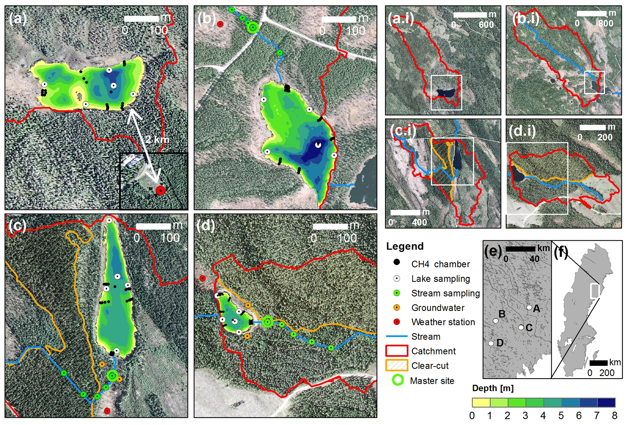
Figure 2Maps of the experimental lakes and streams (a–d), their catchments (a.i–d.i) and their location in Sweden (e–f). Detailed maps show the lake bathymetry; the main channel of the inlet stream; the location of gas concentration sampling sites in lakes, streams, and hillslope groundwater; floating CH4 chambers; and weather stations. Additional physicochemical sampling was done at the master stream site. White frames and dots in smaller-scale maps illustrate the extent or location of corresponding larger-scale maps, respectively. Panel labeling is consistent across all map scales and is as follows: (a) Stortjärn, (b) Övre Björntjärn, (c) Struptjärn, and (d) Lillsjölidtjärnen.
2.3 Water sampling and physicochemical analysis
Surface water was sampled biweekly for dissolved CO2, CH4, and N2O concentrations at stream sites located 40 to 180 m from the lake inlets (hereafter referred to as master stream sites) and the deepest point of the lakes (Fig. 2) as described in Text S1 in the Supplement. Control and impact catchments were typically sampled within 2 or 3 days from each other (but never more than 7 days). To account for temporal variability, surface water CO2 concentrations were also monitored at the deepest point of the lakes and the master stream sites at 2 h intervals using non-dispersive infrared CO2 sensors (see Text S2 for details). To account for spatial variability in CO2 and CH4 concentrations within streams, 300 m long stream transects were sampled at five sites chosen to represent the variability in riparian vegetation and turbulence patterns of the catchment stream. Spatial variability within lakes was accounted for by biweekly sampling of CO2 concentrations at an additional four nearshore locations (Fig. 2). Average nearshore concentrations did not differ from concentrations at the deepest point (linear regression with insignificant intercept and slope = 0.97±0.01, p<0.001, R2=0.99, n=130). Therefore, only data from the deepest point were used for the remainder of this work. Within-lake variability in CH4 concentrations was accounted for by floating-chamber deployments as described further below. In impact catchments, groundwater was sampled biweekly for dissolved inorganic carbon (DIC) and CH4 concentrations from wells at depth-integrated locations (5–105 cm) and depth-specific locations (37.5–42.5 cm). These depths were chosen to separate responses in the whole-soil profile and in shallow groundwater that is tightly connected to streams in our study region (Leith et al., 2015). Wells were located at two forested hillslope sites: one affected by forest clear-cutting, and one serving as an untreated control (Fig. 2, Text S1).
Profiles of dissolved O2 concentrations and photosynthetic active radiation (PAR) were measured biweekly at the deepest point in each lake using handheld probes (ProODO, YSI Inc., Yellow Springs, OH, USA; LI-193 spherical quantum sensor, LI-COR Biosciences, Lincoln, NE, USA). At the deepest point of each lake, at the stream master site, and at the groundwater wells, additional water samples were collected biweekly in acid-washed plastic bottles for physicochemical analysis. At the master stream sites, samples were taken daily by an automatic water sampler (ISCO 6712 full-size portable sampler, Teledyne Inc., Lincoln, NE, USA). At each field visit, a subset of these samples were randomly chosen based on the recorded hydrograph during the past 2-week period: two samples in the absence of flood events and up to four samples before, during, and after a flood event.
We also monitored lake water temperature profiles, stream temperature and discharge, and weather conditions including wind speed, air temperature, precipitation, air pressure, relative humidity, and light intensity at 5–60 min intervals using logger systems described in detail in Text S2. Between 3 % and 12 % of logger data were missing and filled using multiple imputation, linear regression, or linear interpolation methods (see Text S3 and Table S2).
To characterize water color, spectral absorbance at a wavelengths of 420 nm (a420) was measured on filtered lake and stream water (acid-washed Whatman GF/F 0.7 µm) using a spectrophotometer (V-560 UV-VIS, Jasco Inc., Easton, MD, USA). Filtered water from lake, stream, and depth-integrated groundwater sampling was acidified with 500 µL of 1.2 M HCl per 50 mL of sample prior to analysis for DOC and total N (TN) analysis on a total organic analyzer (IL 500 TOC-TN analyzer, Hach, Loveland, CO, USA). For dissolved inorganic nitrogen (DIN = ) analysis, water from lake sampling, stream sampling, and depth-integrated groundwater sampling was filtered through 0.45 µm cellulose acetate filters prior to freezing and analyzed using an automated flow injection analyzer (FIAstar 5000, FOSS, Hillerød, Denmark). All chemical analyses were performed at the Department of Ecology and Environmental Science (EMG), Umeå University. All data analysis described in the following was done using the statistical program R 3.2.2 (R Development Core Team, 2015), if not declared otherwise.
2.4 Lake physics calculations
Lake thermal characteristics were calculated based on 5 min temperature profile data using functions provided by the R-package rLakeAnalyzer (Read et al., 2011). This included epilimnion, hypolimnion and whole-lake mean temperatures; Schmidt stability; the depths of the actively mixing layer (zmix); and the upper and lower boundary of the metalimnion (zupr and zlwr, respectively). For zmix, we chose a density gradient threshold value of 0.1 kg m−3 m−1. Mean O2 concentrations for the epilimnion (water surface to zupr), hypolimnion (zlwr to lake bottom), and the whole lake were then calculated by weighting O2 concentrations by the areal proportion of the depth stratum they represent and integrating these numbers over all depths, following the whole-lake depth-integrated approach by Sadro et al. (2011). Stratum-specific areas were derived from hypsographic curves, established from bathymetric data. Bathymetry data were collected using an echo sounder with an internal GPS antenna (Lowrance HDS-5 Gen2) and interpolated by ordinary kriging (root mean square error (RMSE) = 0.3 m) using the geostatistical analysis package in ArcMap 10.1 (ESRI, Redlands, CA, USA). Light extinction coefficients (kd) were calculated as the slope of the linear regression between natural logarithm of photosynthetically active radiation and depth.
2.5 Gas transfer velocity estimates
For both lakes and streams, gas transfer velocities (k) – the water column depth that equilibrates with the atmosphere per unit time – were expressed as k600, representing CO2 transfer at 20 ∘C water temperature. For lakes, three published k600 models were used to account for prediction uncertainties, including two wind speed based models calibrated for small sheltered lakes (Cole and Caraco, 1998) and boreal lakes of various sizes (Vachon and Prairie, 2013), and a surface renewal model calibrated for small boreal lakes (Heiskanen et al., 2014). Calculations were based on scripts provided by the R-package LakeMetabolizer (Winslow et al., 2016). Measured input variables included wind speed, wind mast height, latitude, lake area, air pressure, air temperature, relative humidity, and surface water temperature. Modeled input variables included kd, zmix, incoming shortwave radiation (sw = lux/244.2, following Kalff, 2002), and net longwave radiation (calculated from measured input variables using the “calc.lw.net.base” function in the R-package “rLakeAnalyzer”; Read et al., 2011). To match temporal resolutions, biweekly kd values were interpolated linearly to 10 min resolution. Wind speed was corrected from mast height to 10 m above ground, assuming a logarithmic wind profile following Crusius and Wanninkhof (2003). To account for uncertainties in k600 estimates for lakes due to gap filling of input variables, we applied a bootstrapping approach (Text S6). For streams, k600 was estimated separately for the four sub-reaches that are bound by the five stream sampling sites. Estimations were based on a total of 23 propane injection experiments and 282 triplicate gas flux chamber measurements carried out at three representative sites per sub-reach (Fig. S1 in the Supplement). Propane injection experiments and flux chamber measurements were repeated 5–10 times per sub-reach during autumn 2013–spring 2015 to cover a wide range of flow conditions (0.01–0.95th, 0.10–0.99th, and 0.25–0.99th percentile of discharge measurements during 1 June–30 September in 2012–2015 in Övre Björntjärn, Struptjärn, and Lillsjölidtjärnen). Details on gas transfer measurements in streams are given in Text S4.
Flux chamber measurements and propane injection experiments were used to establish predictive models of k600 based on stream discharge. Stream discharge was used instead of the more mechanistically relevant variable of flow velocity because both variables were highly correlated (marginal R2=0.71), but only discharge was available at hourly intervals. Hence, hourly k600 was computed for each sub-reach in four steps. First, the arithmetic mean k600 of site-specific flux chamber measurements was calculated for each sub-reach. These sub-reach specific k600 values agreed relatively well with k600 values from propane-injection experiments (R2=0.58, Fig. S2). However, flux chamber measurements were restricted to relatively smooth water surfaces, excluding waterfalls and rapids, and therefore underestimated reach-scale k600 by a factor of 0.61. Second, flux chamber derived k600 was corrected using linear relationships (median R2=0.90) with propane derived k600 whenever they were statistically significant or R2 was >90 %. Third, corrected flux chamber derived k600 was combined with propane derived k600 values to establish sub-reach specific linear regression models that predict k600 based on local discharge (R2=0.56–0.94, Table S3). Whenever the best linear model had a negative intercept, the model was refitted, constraining the intercept to zero to avoid a negatively predicted k600. Fourth, the k600 discharge models were used to predict k600 based on hourly time series of discharge measured at the master stream site and scaled to the respective sub-reach using the mean discharge ratio measured at both sites during propane injection experiments. Throughout these experiments, discharge ratios varied by 5±2 %. To account for uncertainties in k600 estimates for streams, we propagated errors from flux chamber and propane injection experiments and discharge rating curves (Text S6).
2.6 Gas flux estimates
The diffusive gas flux (F) across the lake or stream water interface was calculated using Fick's law:
where cwat is the measured gas concentration of the surface water, ceq is the gas concentration of surface water if it was in equilibrium with ambient air calculated from measured air concentration and water temperature using Henry's constant, and a is the chemical enhancement factor (for CO2 transfer only) set to 1, as enhancement is negligible if pH<8 (Wanninkhof and Knox, 1996). Atmospheric CO2 and N2O concentrations were 425 ppm and 350 ppb (median of biweekly in situ measurements using gas chromatography, Text S1), respectively, and atmospheric CH4 concentrations were below the detection limit of our gas chromatographer (∼3 ppm) and assumed to be 1.893 ppm (http://cdiac.ornl.gov/pns/current_ghg.html, last access: 14 September 2018). The coefficient k was calculated from k600 following Jähne et al. (1987), with the Schmidt coefficient set to −0.5 and gas-specific parameterizations of Schmidt numbers used for in situ water temperature according to Wanninkhof (1992). Errors in F were propagated from standard errors in cwat and k (Fig. S3).
Fluxes of CH4 were measured in 2012 and 2014 using floating chambers according to Bastviken et al. (2010) with the following modifications: 26–32 chambers were placed in each lake to cover five depth zones (water depth 0–1, 1–2, 2–3, 3–4, and >4 m), with one chamber placed at the deepest point and the remainder arranged along depth transects of 3–4 chambers (Fig. 2). Depth transects were chosen to represent the typical shoreline characteristics (inlets, mires, forests). A volume of 50 mL of gas was sampled weekly from June to August from each floating chamber before and after an accumulation period of 24 h using polyethylene syringes. A volume of 30 mL of sampled gas was injected to glass vials (22 mL; PerkinElmer Inc., Waltham, MA, USA) sealed with natural pink rubber stoppers (Wheaton 224100-171) and filled with saturated NaCl solution. During gas transfer, the vials were held upside down to let the excess solution escape through an open syringe needle until around 2 mL solution was left in the vial. To minimize leakage, vials were stored upside down until analysis with a gas chromatograph (7890A, Agilent Technologies, Santa Clara, CA, USA) with a Supelco Porapak Q 80/100 column, a flame ionization detector (FID) and a thermal conductivity detector (TCD) at the Department of Thematic Studies – Environmental Change, Linköping University, Sweden. In addition to chamber sampling, surface water was sampled at the beginning and the end of each 24 h accumulation period in the middle of each transect and analyzed for dissolved CH4 as described above. Chamber-specific total CH4 fluxes were calculated and separated into diffusion and ebullition components using the statistical approach described in Bastviken et al. (2004). Whole-lake fluxes were calculated as the area-weighted mean of depth-zone specific fluxes, which in turn were the arithmetic mean flux of all chambers located at the respective depth.
2.7 Statistical analysis
Clear-cut and site preparation effects were assessed following the paired BACI approach of Stewart-Oaten et al. (1986). To test for “clear-cut” effects, i.e., the general response in the first 3 years after clear-cutting, the “after” period was set to the years 2013–2015. To evaluate whether effects after site preparation differed from general responses, we also tested for “site preparation” effects by setting the after period to the year 2015. The “before” period was always the year 2012. Treatment effects were analyzed in terms of effect sizes (ESs), which are defined as the arithmetic mean change (after − before) in the sampling specific differences between groundwater, stream, or lake pairs (impact-control). The significance of the ES was tested using a linear mixed-effects model (LME) with “paired difference” as the dependent variable and “time” (before-after) as a fixed effect. The factor “pair” was included as a random effect on both slopes and intercepts to account for potential natural variability in responses across the two impact catchments. Reported ESs, slopes, and intercepts are arithmetic means over the pairs. Each impact lake was paired with the arithmetic mean of the control lakes, each impact stream with the control stream, and each impact groundwater sampling site with the respective control site in the impact catchments. All LMEs were analyzed by means of the lme function in the R-package nlme (Pinheiro et al., 2015) using the restricted maximum likelihood approach after BACI model assumptions were evaluated (Text S5). Whenever temporal autocorrelation was significant (Text S5), a first-order autocorrelation term (corAR1, for time series of biweekly observations) or an autoregressive moving-average correlation structure (corARMA, for time series of daily means derived from hourly discharge or 2-hourly CO2 flux data) was included.
Table 2Physicochemical characteristics of lake water, stream water, and groundwater at control and impact sites before and after forest clear-cutting. Also given are the estimated effect sizes (linear mixed-effects model slope), their standard errors (SEs), degrees of freedom (df), t and p values, and Cohen' D, summarized as arithmetic means over ten bootstrap runs that take uncertainty from gap filling into account (see Fig. S3). This uncertainty is expressed as bootstrap standard errors (bse) of p values. Statistically significant p values (<0.05) are highlighted bold. Water levels [cm] are relative to the soil surface. Groundwater data refer to depth-integrated locations (5–105 cm). Abbreviations: Epi is Epilimnion, Hypo is hypolimnion, DOC is Dissolved organic carbon concentration [mg L−1], TN is total nitrogen concentration [µg L−1], DIN is dissolved inorganic nitrogen concentration [µg L−1], a420 is the spectral absorbance at 420 nm [m−1].
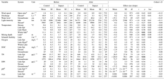
a LME estimates based on log-transformed data.
b Assumption on constancy of paired differences in before period
not met. c Assumption on nonadditivity of paired differences in
before period not met. d Mean and LME estimates
based
on H+ concentrations, SE based on pH
value.
To guarantee homoscedasticity and normality of model residuals, the dependent variables were log + n-transformed if necessary prior to model fitting, where n is the smallest value that leads to normal data when added. To assess the statistical and biogeochemical significance of clear-cutting effects, we used the p value and slope of the LMEs (as an estimate of ES) and Cohen's D, defined as , where s is the standard deviation of paired differences in the before period (Osenberg and Schmitt, 1996). Cohen's D were “small” if D<0.2, “medium” if , and “large” if 0.8≤D. Uncertainties in BACI statistics for gas fluxes and gap-filled logger data were accounted for by combining standard methods of error propagation and bootstrapping (see Text S6 and Fig. S3).
Clear-cut effects on CO2 and CH4 fluxes were also investigated for potential differences along the stream reaches (Fig. 2) depending on the site-specific percentage of the drainage area affected by forest clear-cutting. First, stream-site-specific drainage areas were delineated from a 2 m digital elevation model (DEM) derived from airborne laser scanning (Swedish National Land Survey, 2015) using Hydrology tools in ArcGIS 10.1 (ESRI, Redlands, CA, USA). Modeled flow direction in some ditches were not well represented by the model compared to field observations. In this case, the DEMs were manually corrected (elevation ±20 cm) to emphasize observed ditch flow directions. Next, BACI analyses were performed as described above, where each impact stream site was paired with the respective site in the control stream with respect to the order regarding their distance from the lake inlet. In addition, tests were carried out on linear relationships between the effect size (weighted by SE) of each stream site and the respective percentage of forest clear-cut using an LME with “stream” as random effects on both slopes and intercepts. Here, the dependence of sites within streams was accounted for by setting the alpha level of the statistical analysis to 0.01. Alpha levels of all other statistical analyses were set to 0.05.
3.1 Hydrological and physicochemical response
Forest clear-cuts did not affect riparian groundwater levels or stream discharge (Table 2). Instead, these hydrological characteristics were more regulated by interannual and intra-annual variability in precipitation and snow meltwater inputs. Groundwater levels decreased from 34 to 35 cm depth in the relatively wet before period to 40–42 cm depth in the relatively drier after period (here and hereafter, we refer to arithmetic mean values over each time period; see Table S1 for precipitation data). At the same time, stream discharge decreased from 41 to 27 L s−1 in the control catchment and from 4 to 3 L s−1 in the impact catchments, corresponding to a decrease in specific discharge from 1.5 to 1.0 and 1.1 to 0.9 mm d−1, respectively. Other physical parameters such as wind speed, light intensity, epilimnion and hypolimnion temperature, and Schmidt stability also remained largely unaffected. Light intensities tripled in impact streams (from 3402 to 9969 lux, corresponding to about 14 to 41 W m−2; Kalff, 2002) and showed a “large” effect size. This effect was, however, not significant because of high variability across impact streams (“large” effect in Struptjärn, no change in Lillsjölidtjärnen; stream-specific data not shown). In the impact lakes, whole-lake temperatures increased from 10.7 ∘C in the before period to 11.5 ∘C in the after period, but this increase was 0.4 ∘C less than the increase in the control lakes. Mixing depth decreased from 1.7 to 1.5 m in impact lakes, while it remained at 1.8 m in control lakes. These thermal effects were significant but of “small” size (Table 2).
Table 3Effect size of forest clear-cutting on DIC and CH4 concentrations [µM] in groundwater in the impact catchments as shown in Fig. 3. Given are linear mixed-effects model slope estimates (mean), their standard errors (SEs), degrees of freedom (df), t and p values, and Cohen' D. Statistically significant p values (<0.05) are highlighted bold.
Forest clear-cuts did not affect concentrations of O2, DOC, and DIN in groundwater, stream water, or lake water. Epilimnion and hypolimnion O2 concentrations were around 8 and 1–2 mg L−1, respectively (Table 2). Hypolimnetic water did quickly turn anoxic during summer stratification (Fig. S4). The DOC concentrations ranged from 63 to 77 mg L−1 in groundwater, 25 to 29 mg L−1 in streams, and 18 to 21 mg L−1 in lakes (Table 2). Concentrations of DIN ranged from 467 to 538 µg L−1 in groundwater, 21 to 32 µg L−1 in stream water, and 14 to 20 µg L−1 in lake water. Concentrations of TN decreased in impact streams from 595 to 505 µg L−1; this is a significant “medium” size effect relative to the increase in control streams from 498 to 531 µg L−1. However, TN remained unaffected in groundwater (1572–1958 µg L−1) and lake water (367 to 446 µg L−1). Spectral absorbance at 420 nm ranged from 12 to 15 m−1 in streams and 9 to 13 m−1 in lakes and was not affected by clear-cutting. However, pH showed a significant BACI effect and increased more in control systems compared to impact systems in the after period relative to the before period: from 3.9 to 4.8 in the control stream and from 4.4 to 4.6 in the impact streams, and from 4.2 to 5 in control lakes and from 5.1 to 5.4 in the impact lakes (Table 2).
Most hydrological and physicochemical parameters remained unaffected by the treatment even after site preparation (Table S4). The only significant BACI effects concerned “medium” size decreases in stream pH and increases in stream DIN concentrations, and “small” or “medium” size decreases in hypolimnetic and whole-lake temperatures and mixing depths and increases in Schmidt stability.
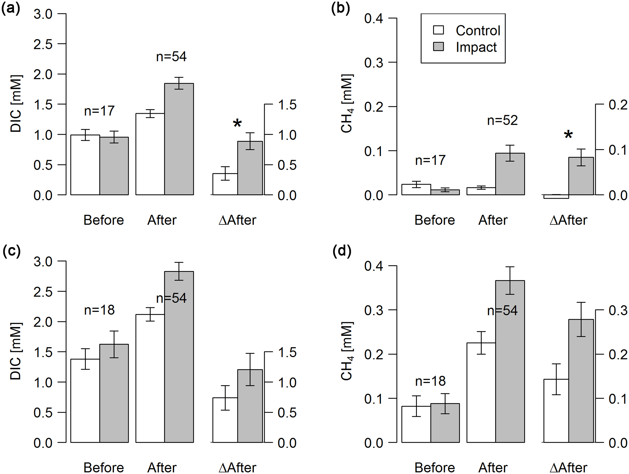
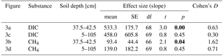
Figure 3Concentrations of DIC and dissolved CH4 in groundwater at depth-specific locations (37.5–42.5 cm; a–b) and depth-integrated locations (5–105 cm; c–d) before and after clear-cutting at impact sites, and the respective differences between before and after (ΔAfter, shown in the same units). Each bar represents mean values (±propagated standard errors) of repeated observations over time. Significant (p<0.05) effect sizes are marked by an asterisk. Abbreviations: n is the number of observations.

Figure 4Time series of lake–atmosphere CO2 fluxes based on daily means of 2-hourly concentration measurements (grey lines), biweekly spot measurements (blue dots), and the k model by Cole and Caraco (1998). Given are absolute fluxes and differences (ΔCO2) between impact and control lakes. Shadings and error bars show propagated standard errors (see Fig. S3 and Text S6). Gap-filled data are colored in red. Bars show the lake ice cover duration with uncertainties expressed by grey scale (dark = minimum duration, light = maximum duration). Dashed lines mark the timing of forest clear-cutting (2013) and site preparation (2014). Units are consistent across all panels. Abbreviations: SR is Stortjärn, OB is Övre Björntjärn, ST is Struptjärn, and LL is Lillsjölidtjärnen.
3.2 Response of GHG concentrations
Groundwater DIC and CH4 concentrations increased in response to forest clear-cutting. Specifically, in shallow groundwater (37.5–42.5 cm), DIC concentrations increased from 992 to 1345 µM at control sites but from 957 to 1846 µM at impact sites; this is a significant “medium” effect size of +533 µM or +56 % relative to the impact sites in the control year (Fig. 3a, Table 3). Whole-soil profile (5–105 cm) DIC concentrations increased at similar rates “medium” effect size of +458 µM), yet this change was not statistically significant (Fig. 3c, Table 3). CH4 concentrations in shallow groundwater decreased from 24 to 16 µM in control sites but increased from 11 to 94 µM at impact sites; this is a significant “large” effect size of +93 µM or +822 % relative to the impact sites in the control year (Fig. 3b, Table 3). Whole-soil profile CH4 concentrations increased at even larger absolute rates (+139 µM), but this change was only of “medium” size and not statistically significant due to high variability (Fig. 3d, Table 3).
Table 4Effect size of forest clear-cutting on fluxes of CO2, CH4, and N2O across the interface between lakes or streams and the atmosphere as shown in Figs. 6 and 7. Shown are linear mixed-effects model slope estimates, their standard errors (SEs), degrees of freedom (df), t and p values, and Cohen' D, summarized as arithmetic means over ten bootstrap runs that take uncertainty from gap-filling and gas flux models into account (see Fig. S3). This uncertainty is expressed as bootstrap standard errors (bse) of p values. For lake–atmosphere fluxes, estimates based on three different k models are shown. Note that parameter estimates are based on log+n transformed data, where n is the smallest number that, when added, leads to positive normal values. Abbreviations: Logger is the daily mean of 2-hourly measurements, Chamber is the floating chamber, and Spot is the spot measurement.
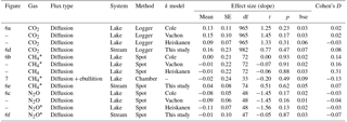
* Assumption on nonadditivity of paired differences in before period not met.
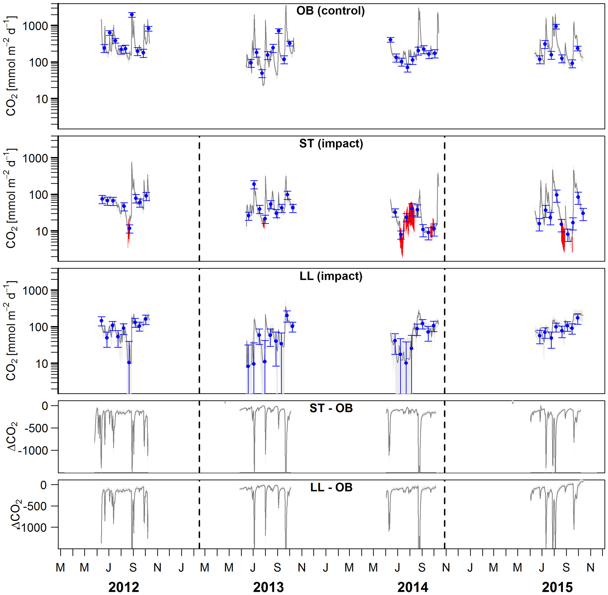
Figure 5Time series of stream–atmosphere CO2 fluxes based on daily means of 2-hourly concentration measurements (dark grey lines) and biweekly spot measurements ±standard errors (blue dots and error bars). Given are absolute fluxes and differences (ΔCO2) between impact and control streams. Shadings and error bars show propagated standard errors (see Fig. S3 and Text S6). Gap-filled data are colored in red. Dashed lines mark the timing of forest clear-cutting (2013) and site preparation (2014). Units are consistent across all panels. Abbreviations: SR is Stortjärn, OB is Övre Björntjärn, ST is Struptjärn, and LL is Lillsjölidtjärnen.
Site preparation did not cause any additional effects on groundwater DIC and CH4 concentrations (Table S5). However, effect sizes remained at “medium” (+518 to +799 µM) and “large” levels (+69 to +208 µM), respectively, and DIC in shallow groundwater was still significantly elevated relative to reference conditions.
In streams and lakes, CO2 concentrations were between 269 and 349, and 95 and 109 µM; CH4 concentrations between 0.2 and 3.4 and between 0.3 and 1.1 µM; and N2O concentrations between 16 and 22 nM and between 12 and 17 nM, respectively (Table S6). Stream and lake water GHG concentrations did not respond to forest clear-cutting or site preparation, except for stream CO2 that increased less in impact streams (from 314 to 349 µM after clear-cutting and 329 µM after site preparation) relative to the control stream (from 269 to 347 and 314 µM, respectively).
3.3 Response of GHG emissions from streams and lakes
Lakes and streams emitted CO2, CH4, and N2O to the atmosphere, but the fluxes did not respond to forest clear-cutting. For CO2 fluxes, this observation is based on daily averages of 2-hourly time series shown in Figs. 4 and 5. CO2 fluxes varied synchronously across all lakes at daily and seasonal timescales, with emission events during storms and a general increase towards autumn (Fig. 4). Daily means of 2-hourly estimates were validated by estimates based on biweekly spot measurements (LME, slope = 0.97±0.03, p<0.001, marginal R2=0.87, residual standard error (rse) = 9.9 mmol m−2 d−1, n=180). Time series of the differences between impact and control lakes did not reveal any systematic change in offset or seasonality between the before and after period. Depending on the k model chosen, seasonal mean CO2 fluxes varied between 41 and 99 mmol m−2 d−1. However, consistent for all models, there was no significant BACI effect associated with forest clear-cuts (Fig. 6a, Table 4) or site preparation (Table S7).

Figure 6Fluxes of CO2, CH4, and N2O across the interface between lakes (a–c) or streams (d–f) and the atmosphere in control and impact catchments before and after forest clear-cutting, and the respective differences between before and after (ΔAfter, shown in the same units). Each bar represents mean values (±propagated standard errors) of repeated observations over time, summarized as arithmetic means over ten bootstrap runs that take uncertainty from gap-filling and gas flux models into account (see Fig. S3 and Text S6). Data are based on daily means of 2-hourly measurements (CO2) or biweekly (CH4 and N2O) concentration measurements. Lake–atmosphere fluxes are here calculated using the k model by Cole and Caraco (1998). Abbreviations: n is the number of observations.
In streams, 2-hourly time series revealed pronounced CO2 emission peaks during storm events (Fig. 5). These emission peaks were strikingly synchronous between streams, but peak amplitudes varied from around 200 to up to 2000 mmol m−2 d−1 (Fig. 5). Between-stream differences did not change in the after period relative to the before period, indicated by nonsignificant BACI effects associated to forest clear-cutting (Table 4) and site preparation (Table S7). Daily means of 2-hourly emission estimates were validated by estimates based on biweekly spot measurements with excellent agreement (LME, slope = 1.05±0.01, p<0.001, marginal R2=0.97, rse = 28.3 mmol m−2 d−1, n=180).
Seasonal means of diffusive CH4 fluxes across the lake–atmosphere interface also varied depending on the k model chosen (between 0.17 and 0.81 mmol m−2 d−1), but regardless of model choice there was no significant BACI effect associated with forest clear-cuts (Fig. 6b, Table 4) or site preparation (Table S7). This result, derived from spot measurements during June–September at the deepest point of the lake, was also confirmed for total CH4 fluxes (including ebullition) by independent weekly measurements using floating chambers deployed across the whole lake during mid-June to late August (Fig. 7, Table 4). Accordingly, total CH4 fluxes integrated over the whole lake surface varied from 0.22 to 0.52 mmol m−2 d−1, of which 72 %–82 % was due to ebullition and the remainder due to diffusion. Diffusive CH4 fluxes across the stream–atmosphere interface varied from 1.2 to 1.3 mmol m−2 d−1 in the control stream and from 0.07 to 0.18 mmol m−2 d−1 in the impact streams (Fig. 6e) and remained unaffected by forest clear-cutting or site preparation (Tables 4, S7).
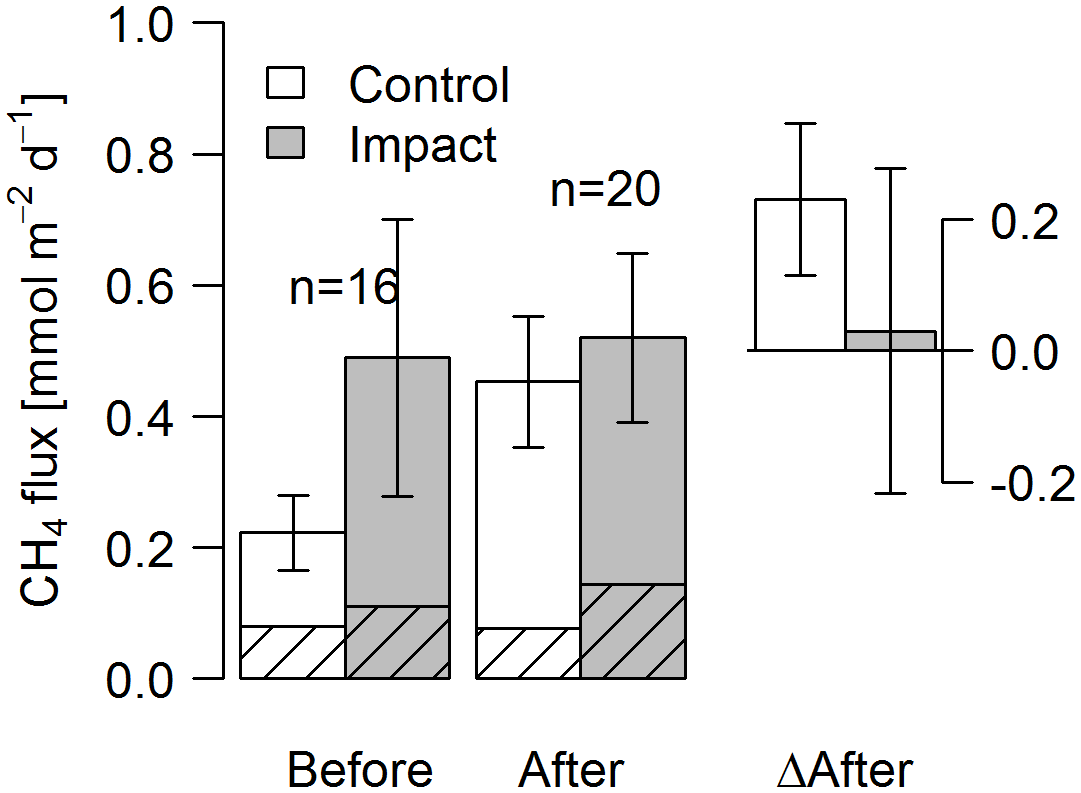
Figure 7Fluxes of CH4 by diffusion (shaded) and ebullition (non-shaded) across the lake–atmosphere interface in control and impact catchments before and after forest clear-cutting, and the respective differences between before and after (ΔAfter, shown in the same units). Fluxes were measured by the use of flux chambers (e.g., independent approach compared to fluxes calculated from concentrations in Fig. 6). Each bar represents mean values (±propagated standard errors) of whole-lake fluxes measured weekly from mid-June to mid-August 2012 and 2014, summarized as arithmetic means over ten bootstrap runs that take between-chamber variability into account (see Fig. S3 and Text S6). Whole-lake fluxes are the area-weighted mean of depth-zone specific fluxes. Abbreviations: n is the number of observations.

Figure 8Fluxes of (a) CO2 and (c) CH4 across the stream–atmosphere interface along stream transects in the control catchment (C) and two impact catchments (I) before and after forest clear-cutting (OB = Övre Björntjärn, ST = Struptjärn, LL = Lillsjölidtjärnen,). Effect sizes (ES) defined as the before–after change in the difference between control and impact streams are shown in panels (b) and (d). Each point represents seasonal mean values (±standard errors) of biweekly observations, summarized as arithmetic means over ten bootstrap runs that take uncertainty from gap-filling and gas flux models into account (see Fig. S3 and Text S6).
Across five sites sampled along 300 m long stream reaches, CO2 and CH4 fluxes varied from 43 to 465 and from −0.02 to 5.43 mmol m−2 d−1, respectively (Fig. 8a, c). BACI effect sizes were “small” but had a large variability ranging from −53 to 295 and −4.32 to 0.27 mmol m−2 d−1 (Fig. 8b, d, Table S8). These effect sizes were nonsignificant across the whole length of both impact stream reaches and did not vary across the clear-cut gradient, with a 5-fold increase in the areal proportion of the stream reach drainage area affected by forest clear-cutting (LME, slope = 10.9±5.3 mmol CO2 m−2 d−1 % clear-cut−1, t=2.06, p=0.08, marginal R2=0.34, and 0.002±0.003 mmol CH4 m−2 d−1 % clear-cut−1, t=0.54, p=0.61, marginal R2=0.03, respectively).
Seasonal means of diffusive N2O fluxes across the lake–atmosphere interface varied, depending on the k model chosen, between 0.4 and 3.5 µmol m−2 d−1. Consistent for all k models, there was no significant BACI effect associated with forest clear-cuts (Fig. 6c, Table 4). The same was true for diffusive N2O fluxes across the stream–atmosphere interface, ranging from 1.7 to 3.5 µmol m−2 d−1 (Fig. 6f, Table 4).
This study is to our knowledge the first experimental assessment of forest clear-cut and site preparation effects on GHG fluxes between inland waters and the atmosphere and expands on previous forest clear-cutting experiments that primarily have focused on effects on hydrology or water chemistry. Our whole-catchment BACI experiment showed no significant initial effects of forest clear-cutting and site preparation on GHG fluxes in streams or lakes despite enhanced potential GHG supply from hillslope groundwater. This suggests that the generally strong effects of clear-cut forestry on terrestrial C and nutrient cycling are not necessarily translated to major effects in GHG emissions from recipient downstream aquatic ecosystems. Our results are representative for low-productive boreal forest systems (< 3 m3 ha−1 yr−1) in relatively flat landscapes, which represent the dominant forest type subject to clear-cut forestry in the boreal biome (Zheng et al., 2004; SFA, 2014).
What caused the contrasting response in GHGs between groundwater and open water? Open water CO2, CH4, and N2O can result from bacterial degradation of organic matter (Bogard and del Giorgio, 2016; Hotchkiss et al., 2015; Peura et al., 2014) and incomplete denitrification and nitrification (McCrackin and Elser, 2010; Seitzinger, 1988), respectively. These processes are connected to DOC and DIN dynamics. The lack of initial responses in catchment-derived DOC and DIN could, therefore, explain the lack of responses in aquatic GHG fluxes. However, aquatic GHG fluxes are also fueled by direct catchment inputs of the respective dissolved gases (Rasilo et al., 2017; Striegl and Michmerhuizen, 1998; Öquist et al., 2009). Groundwater CO2 and CH4 concentration increased in response to the clear-cut treatment (Fig. 3), potentially as a consequence of enhanced organic matter degradation due to enhanced post-clear-cut soil temperatures (Bond-Lamberty et al., 2004; Schelker et al., 2013a) or reduced CH4 oxidation (Bradford et al., 2000; Kulmala et al., 2014). Some CO2 and CH4 may be formed from degradation of logging residues and litter in the soil (Mäkiranta et al., 2012; Palviainen et al., 2004). However, it is presently unclear whether this source has contributed to enhanced groundwater CO2 and CH4 concentrations. Concentration increases were most pronounced in shallow groundwater, the hotspot for riparian GHG export to headwater streams in our study region (Leith et al., 2015). Considering that clear-cut areas covered on average ∼30 % of the stream and lake catchments, but ∼80 % of the subcatchments of the groundwater sampling sites, the 56 % increase in groundwater CO2 concentrations could have caused an increase of at most 21 % () in CO2 concentrations in the impact streams and lakes. Part of the lack of a response could be due to difficulties in detecting such subtle changes given the relatively high natural variability (Table S6). However, the 8-fold increase in groundwater CH4 concentrations could have supported at most 3-fold increases () in CH4 concentrations in streams and lakes, much larger than those observed in our study (Table S6). This mismatch suggests the following three alternative explanations.
First, groundwater-derived GHGs were transport-limited and, hence, only a minor source for GHG fluxes in our lakes and streams. Even though external sources often dominate CO2 and CH4 emissions in headwater streams (Hotchkiss et al., 2015; Öquist et al., 2009; Jones and Mulholland, 1998), soil-derived gases may only be a minor source for GHGs in headwaters during summer low-flow conditions (Dinsmore et al., 2009; Rasilo et al., 2017). Such conditions were present over extended parts during the dry post-treatment period (Tables S1, S4).
Second, the riparian zone effectively buffered potential clear-cut and site preparation effects on aquatic GHG fluxes. In part, this could be because the riparian buffer zones were wide enough to retain their wind sheltering function. Wind speeds indeed remained unaffected by clear-cutting on nearby mires (Table 2). This would indicate that riparian buffer zones may have prevented additional forcing on air–water gas exchange velocities, assuming that relative changes in wind speeds on the mires were representative for lake conditions (Text S2). In addition, riparian zones may have acted as efficient reactors of GHGs and reduced their concentration during transport from the hillslope to the open water (Leith et al., 2015; Rasilo et al., 2017, 2012). This applies especially to methane, which can be efficiently oxidized in the large redox gradients in riparian zones, similar to inorganic N (Blackburn et al., 2017).
Third, in-stream processing effectively buffered potential clear-cut and site preparation effects on aquatic GHG fluxes. In boreal headwater streams, metabolism can strongly regulate CO2 emissions at summer low-flow conditions (Rasilo et al., 2017). Therefore, additional CO2 leaking from clear-cut soils could have been taken up by algae stimulated in growth by increased light intensities (Kiffney et al., 2003; Clapcott and Barmuta, 2010). We indeed observed strong algae blooms in the inlet stream of Struptjärn in response to a tripling in light intensities after forest clear-cutting (Fig. S5). Increased algal CO2 and N uptake could explain the observed decrease in stream CO2 and TN concentrations. In the experimental lakes, however, we did not observe any change in primary production in response to the treatment (Deininger et al., 2018). Additional CH4 transported from clear-cut soils could have been efficiently oxidized. Enhanced in-stream CH4 oxidation in the sediments is likely primarily an effect of the commonly found substrate limitation of CH4 oxidation (e.g., Bastviken, 2009; Duc et al., 2010; Segers, 1998), i.e., CH4 oxidizer communities have a higher capacity than commonly expressed and will oxidize more CH4 when concentrations increase. Despite lacking mechanistic understanding of the biogeochemical function of the riparian zones and headwater streams in our catchments, we can conclude from groundwater, stream, and lake observations that they must have effectively prevented the potential increase in aquatic GHG emissions. In addition, the riparian buffer vegetation left aside could have acted as wind shelters that prevented potential increases in emissions due to enhanced near-surface turbulence. However, the biogeochemical processing of GHGs in the riparian zone–stream continuum should be given special attention in future clear-cut experiments to resolve the mismatch between responses in hillslope groundwater and receiving streams and lakes.
Our experiment revealed statistically significant BACI effects on pH and lake thermal conditions. The relative pH decrease of 0.5 units in impact relative to control systems is a common clear-cut effect in northern forests (Martin et al., 2000; Tremblay et al., 2009). However, most relevant for the scope of this paper, this change did not bias CO2 concentrations because shifts in the bicarbonate buffer system are minor (≤2 %) at the observed pH levels of ≤5 (Stumm and Morgan, 1995). Likewise, pH is not a major control on aquatic CH4 cycling (Stanley et al., 2016). This applies even to N2O here, because we did not observe any increase in N2O emissions in the post-clear-cut period that would be expected from the positive effect of higher pH levels on nitrification (Soued et al., 2016). Whole-lake temperatures and mixing depths decreased significantly in impact lakes relative to control lakes. However, these effects were small in absolute terms (−0.4 ∘C, −0.2 m, respectively) and associated with relative epilimnion volume changes of about 10 %. Such subtle changes are unlikely to have had major effects on metabolism and lake-internal vertical exchange processes as a driver of GHG fluxes.
In contrast to many previous boreal forest clear-cut experiments (Schelker et al., 2012; Nieminen, 2004; Lamontagne et al., 2000; Winkler et al., 2009; Bertolo and Magnan, 2007; Palviainen et al., 2014), hydrology and water chemistry remained largely unaffected by our treatments. The absence of effects is no absolute evidence of an absence of impacts, but the response is low relative to natural variability and restricted to initial responses within 3 years after clear-cutting. First, hydrological responses may have been masked or delayed given that the post-clear-cut period was much dryer than the pre-clear-cut period (Buttle and Metcalfe, 2000; Schelker et al., 2013b; Kreutzweiser et al., 2008). During the post-clear-cut period, groundwater levels may have fallen below a threshold level in both control and impact catchments where any minor clear-cut induced increase in water levels would not have translated into comparable increases in stream discharge. This is because stream discharge largely depends on the transmissivity which typically decreases exponentially with depth in Swedish boreal soils (Bishop et al., 2011). Second, the proportion of clear-cuts in our catchments (18 %–44 %) was just around the threshold level (∼30 %), above which significant effects on hydrology and water chemistry can be expected in our study region (Ide et al., 2013; Palviainen et al., 2014; Schelker et al., 2014). These threshold values can however vary and are highly site-specific (Kreutzweiser et al., 2008; Palviainen et al., 2015). For example, the relatively high baseline DOC concentrations in our streams and lakes (20 and 29 mg L−1, respectively) are potentially less likely to be further enhanced by forest clear-cuts. Relatively wide riparian buffer strips and gentle catchment slopes (Table 1) may have further dampened these effects (Kreutzweiser et al., 2008). Third, the time it takes for the system to respond may have exceeded the experimental period. For example, it can take 4 to 10 years for groundwater nitrate concentrations to respond to clear-cutting in low-productive forest ecosystems due to tight terrestrial N cycling (Futter et al., 2010). Similar delays have been found for responses in boreal stream and lake water chemistry, often triggered by site preparation (Schelker et al., 2012; Palviainen et al., 2014). In the first year after site preparation, only stream DIN concentrations started to increase, but not DOC or GHG concentrations. However, the absence of initial effects does not necessarily imply absence of longer-term effects. On decadal timescales, forestry may change soil C cycling (Diochon et al., 2009), leading to enhanced terrestrial organic matter exports and lake CO2 emissions (Ouellet et al., 2012). Clearly, future work should explore how universal our results are across different hydrological conditions, other types of systems, and longer timescales.
The particular complexity and multiple controls of catchment-scale GHG fluxes emphasize the need of large-scale experiments to assess treatment responses in realistic natural settings (Schindler, 1998). We addressed this challenge by sampling at high spatial and temporal resolution. However, logistical challenges forced us to restrict the analysis to 1 June to 30 September, the period for which we were able to collect consistent data in all years and all catchments. Hence, we do not account for potential clear-cut effects on stream–atmosphere fluxes during snowmelt (April–May) or late autumn storms (October–November), when a large proportion of GHGs in streams can be supplied from catchment soils (Leith et al., 2015; Dinsmore et al., 2013). Similarly, we do not account for potential clear-cut effects on lake–atmosphere fluxes during ice-breakup (mid-May), which can be fueled by gases directly derived from catchment inputs or be a result of degradation of catchment-derived organic matter during winter (Denfeld et al., 2015; Vachon et al., 2017). Peak flow conditions during spring or late autumn are hot moments of clear-cut effects on C and N export to aquatic systems (Schelker et al., 2016; Laudon et al., 2009; Ide et al., 2013). Spring can also contribute disproportionally to annual GHG fluxes of boreal headwater streams (Dinsmore et al., 2013; Natchimuthu et al., 2017) and lakes (Huotari et al., 2009; Karlsson et al., 2013). Strong seasonality in CO2 fluxes was also apparent in our systems (Figs. 4, 5). Hence, future investigations of clear-cut effects should be based on whole-year sampling.
In summary, our experiment shows for the first time that air–water GHG fluxes in lakes and streams during the summer season do not respond initially to catchment forest clear-cutting and site preparation, despite increases in the potential supply of CO2 and CH4 from clear-cut affected catchment soils. These results suggest that the riparian buffer zone–stream continuum likely acted as a biogeochemical reactor or wind shelter and by that, effectively prevented treatment-induced increases in aquatic GHG emissions. Our findings apply to initial effects (3 years) in low-productive boreal forest systems with relatively flat terrain, where a modest but realistic treatment (18 %–44 % of lake catchments clear-cut) caused only limited effects on catchment hydrology and biogeochemistry.
All data shown in Figures in the main document are provided in the Supplement (Files S1–S5).
Supplement contains extended methods (Texts S1–S6), eight tables (Tables S1–S8), and five figures (Figs. S1–S5).
The supplement related to this article is available online at: https://doi.org/10.5194/bg-15-5575-2018-supplement.
JKa and AKB designed the study with contributions from JKl, DB and HL. MK, EG and AJ performed the fieldwork. MK analyzed the data with contributions from EG. MK wrote the manuscript. All co-authors revised the paper.
The authors declare that they have no conflict of interest.
We thank Henrik Reyier and Ingrid Sundgren for the analysis of floating chamber
CH4 samples; Anne Deininger, Sonja Prideaux, Maria Myrstener,
Antonio Aguilar, Linda Lundgren, William Lidberg, Daniel Karlsson,
Björn Skoglund, Martin Tarberg, Maria Sandström, Linda Engström,
Pär Geibrink, Jonas Gustafsson, Martin Johansson, Leverson Chavez,
Karina Tôsto, Jamily Almeida, Luísa Dantes, Luana Pinho, and
Bernardo Papi for field and lab assistance; Alex Enrich-Prast for logistical
help; Marcus Wallin and Dominic Vachon for discussions on gas transfer
velocity measurements and models; and Peter A. Staehr for comments on an
earlier version of this paper. Forestry practices were carried out by
the companies Svenska Cellulosa AB (SCA) and Sveaskog AB. We thank
Karin Valinger Aggeryd (SCA) and Anders Eriksson (Sveaskog AB) for help with
logistics and catchment selection. This work was supported by the Swedish
Research Councils Formas (grant no. 210-2012-1461), Kempestiftelserna (grant
no. SMK-1240) with grants awarded to Jan Karlsson, and VR (grant no.
2012-00048), STINT (grant no. 2012-2085), and the European Research Council
(grant no. 725546) with grants awarded to David Bastviken.
Edited by: Lutz Merbold
Reviewed by: two
anonymous referees
Andréassian, V.: Waters and forests: From historical controversy to scientific debate, J. Hydrol., 291, 1–27, https://doi.org/10.1016/j.jhydrol.2003.12.015, 2004.
Ask, J., Karlsson, J., and Jansson, M.: Net ecosystem production in clear-water and brown-water lakes, Global Biogeochem. Cy., 26, 1–7, https://doi.org/10.1029/2010GB003951, 2012.
Bastviken, D.: Methane, in: Encyclopedia of Inland Waters, edited by: Likens, G. E., Elsevier, Oxford, 2009.
Bastviken, D., Cole, J., Pace, M., and Tranvik, L.: Methane emissions from lakes: Dependence of lake characteristics, two regional assessments, and a global estimate, Global Biogeochem. Cy., 18, 1–12, https://doi.org/10.1029/2004GB002238, 2004.
Bastviken, D., Cole, J. J., Pace, M. L., and Van de-Bogert, M. C.: Fates of methane from different lake habitats: Connecting whole-lake budgets and CH4 emissions, J. Geophys. Res.-Biogeo., 113, 1–13, https://doi.org/10.1029/2007JG000608, 2008.
Bastviken, D., Santoro, A. L., Marotta, H., Pinho, L. Q., Calheiros, D. F., Crill, P., and Enrich-Prast, A.: Methane emissions from pantanal, South America, during the low water season: Toward more comprehensive sampling, Environ. Sci. Technol., 44, 5450–5455, https://doi.org/10.1021/es1005048, 2010.
Battin, T. J., Luyssaert, S., Kaplan, L. A., Aufdenkampe, A. K., Richter, A., and Tranvik, L. J.: The boundless carbon cycle, Nat. Geosci., 2, 598–600, https://doi.org/10.1038/ngeo618, 2009.
Bergström, A. K. and Jansson, M.: Atmospheric nitrogen deposition has caused nitrogen enrichment and eutrophication of lakes in the northern hemisphere, Glob. Change Biol., 12, 635–643, https://doi.org/10.1111/j.1365-2486.2006.01129.x, 2006.
Bertolo, A. and Magnan, P.: Logging-induced variations in dissolved organic carbon affect yellow perch (Perca flavescens) recruitment in Canadian Shield lakes, Can. J. Fish. Aquat. Sci., 64, 181–186, https://doi.org/10.1139/f07-004, 2007.
Bishop, K., Seibert, J., Nyberg, L., and Rodhe, A.: Water storage in a till catchment. II: Implications of transmissivity feedback for flow paths and turnover times, Hydrol. Process., 25, 3950–3959, https://doi.org/10.1002/hyp.8355, 2011.
Blackburn, M., Ledesma, J. L. J., Näsholm, T., Laudon, H., and Sponseller, R. A.: Evaluating hillslope and riparian contributions to dissolved nitrogen (N) export from a boreal forest catchment, J. Geophys. Res.-Biogeo., 122, 324–339, https://doi.org/10.1002/2016JG003535, 2017.
Bogard, M. J. and del Giorgio, P. A.: The role of metabolism in modulating CO2 fluxes in boreal lakes, Global Biogeochem. Cy., 30, 1509–1525, https://doi.org/10.1002/2016GB005463, 2016.
Bogard, M. J., del Giorgio, P. A., Boutet, L., Chaves, M. C. G., Prairie, Y. T., Merante, A., and Derry, A. M.: Oxic water column methanogenesis as a major component of aquatic CH4 fluxes, Nat. Commun., 5, 5350, https://doi.org/10.1038/ncomms6350, 2014.
Bond-Lamberty, B., Wang, C., and Gower, S. T.: Net primary production and net ecosystem production of a boreal black spruce wildfire chronosequence, Glob. Change Biol., 10, 473–487, https://doi.org/10.1111/j.1529-8817.2003.0742.x, 2004.
Bradford, M. A., Ineson, P., Wookey, P. A., and Lappin-scott, H. M.: Soil CH 4 oxidation?: response to forest clearcutting and thinning, Soil Biol. Biochem., 32, 1035–1038, 2000.
Buttle, J. M. and Metcalfe, R. A.: Boreal forest disturbance and streamflow response, northeastern Ontario, Can. J. Fish. Aquat. Sci., 57, 5–18, https://doi.org/10.1139/cjfas-57-S2-5, 2000.
Clapcott, J. E. and Barmuta, L. A.: Forest clearance increases metabolism and organic matter processes in small headwater streams, J. N. Am. Benthol. Soc., 29, 546–561, https://doi.org/10.1899/09-040.1, 2010.
Cole, J. J. and Caraco, N. F.: Atmospheric exchange of carbon dioxide in a low-wind oligotrophic lake measured by the addition of SF6, Limnol. Oceanogr., 43, 647–656, https://doi.org/10.4319/lo.1998.43.4.0647, 1998.
Cole, J. J., Prairie, Y. T., Caraco, N. F., McDowell, W. H., Tranvik, L. J., Striegl, R. G., Duarte, C. M., Kortelainen, P., Downing, J. A., Middelburg, J. J., and Melack, J.: Plumbing the global carbon cycle: Integrating inland waters into the terrestrial carbon budget, Ecosystems, 10, 171–184, https://doi.org/10.1007/s10021-006-9013-8, 2007.
Crusius, J. and Wanninkhof, R.: Gas transfer velocities measured at low wind speed over a lake, Limnol. Oceanogr., 48, 1010–1017, 2003.
Dawson, J. J. C. and Smith, P.: Carbon losses from soil and its consequences for land-use management, Sci. Total Environ., 382, 165–190, https://doi.org/10.1016/j.scitotenv.2007.03.023, 2007.
Deininger, A., Jonsson, A., Karlsson, J., and Bergström, A.-K.: Low response of humic lake food web to forest clear cutting, Ecol. Appl., 2018.
Denfeld, B. A., Wallin, M. B., Sahlée, E., Sobek, S., Kokic, J., Chmiel, H. E., and Weyhenmeyer, G. A.: Temporal and spatial carbon dioxide concentration patterns in a small boreal lake in relation to ice cover dynamics, Boreal Environ. Res., 20, 679–692, 2015.
Deutzmann, J. S., Stief, P., Brandes, J., and Schink, B.: Anaerobic methane oxidation coupled to denitrification is the dominant methane sink in a deep lake, P. Natl. Acad. Sci. USA, 111, 18273–18278, https://doi.org/10.1073/pnas.1411617111, 2014.
Dinsmore, K. J., Billet, M. F., and Moore, T. R.: Transfer of carbon dioxide and methane through the soil-water-atmosphere system at Mer Bleue peatland, Canada, Hydrol. Process., 23, 330–341, https://doi.org/10.1002/hyp.7158, 2009.
Dinsmore, K. J., Wallin, M. B., Johnson, M. S., Billett, M. F., Bishop, K., Pumpanen, J., and Ojala, A.: Contrasting CO2 concentration discharge dynamics in headwater streams: A multi-catchment comparison, J. Geophys. Res.-Biogeo., 118, 445–461, https://doi.org/10.1002/jgrg.20047, 2013.
Diochon, A., Kellman, L., and Beltrami, H.: Looking deeper: An investigation of soil carbon losses following harvesting from a managed northeastern red spruce (Picea rubens Sarg.) forest chronosequence, Forest Ecol. Manag., 257, 413–420, https://doi.org/10.1016/j.foreco.2008.09.015, 2009.
Duc, N. T., Crill, P., and Bastviken, D.: Implications of temperature and sediment characteristics on methane formation and oxidation in lake sediments, Biogeochemistry, 100, 185–196, https://doi.org/10.1007/s10533-010-9415-8, 2010.
France, R., Steedman, R., Lehmann, R., and Peters, R.: Landscape modification of DOC concentration in boreal lakes: implications for UV-B sensitivity, Water, Air Soil Pollut., 122, 153–162, 2000.
Futter, M. N., Ring, E., Högbom, L., Entenmann, S., and Bishop, K. H.: Consequences of nitrate leaching following stem-only harvesting of Swedish forests are dependent on spatial scale, Environ. Pollut., 158, 3552–3559, https://doi.org/10.1016/j.envpol.2010.08.016, 2010.
Goodale, C. L., Apps, M. J., Birdsey, R. A., Field, C. B., Heath, L. S., Houghton, R. A., Jenkins, J. C., Kohlmaier, G. H., Kurz, W., Liu, S., Nabuurs, G., Nilsson, S., and Shvidenko, A. Z.: Forest Carbon Sinks in the Northern Hemisphere, Ecol. Appl., 12, 891–899, https://doi.org/10.1890/1051-0761(2002)012[0891:FCSITN]2.0.CO;2, 2002.
Heiskanen, J. J., Mammarella, I., Haapanala, S., Pumpanen, J., Vesala, T., Macintyre, S., and Ojala, A.: Effects of cooling and internal wave motions on gas transfer coefficients in a boreal lake, Tellus B, 66, 1–16, https://doi.org/10.3402/tellusb.v66.22827, 2014.
Hotchkiss, E. R., Hall Jr., R. O., Sponseller, R. A., Butman, D., Klaminder, J., Laudon, H., Rosvall, M., and Karlsson, J.: Sources of and processes controlling CO2 emissions change with the size of streams and rivers, Nat. Geosci., 8, 696–699, https://doi.org/10.1038/ngeo2507, 2015.
Houser, J. N., Bade, D. L., Cole, J. J., and Pace, M. L.: The dual influences of dissolved organic carbon on hypolimnetic metabolism: Organic substrate and photosynthetic reduction, Biogeochemistry, 64, 247–269, https://doi.org/10.1023/A:1024933931691, 2003.
Huotari, J., Ojala, A., Peltomaa, E., Pumpanen, J., Hari, P., and Vesala, T.: Temporal variations in surface water CO2 concentration in a boreal humic lake based on high-frequency measurements, Boreal Environ. Res., 14, 48–60, 2009.
Huttunen, J. T.: Nitrous oxide flux to the atmosphere from the littoral zone of a boreal lake, J. Geophys. Res., 108, 4421, https://doi.org/10.1029/2002JD002989, 2003.
Huttunen, J. T., Alm, J., Liikanen, A., Juutinen, S., Larmola, T., Hammar, T., Silvola, J., and Martikainen, P. J.: Fluxes of methane, carbon dioxide and nitrous oxide in boreal lakes and potential anthropogenic effects on the aquatic greenhouse gas emissions, Chemosphere, 52, 609–621, https://doi.org/10.1016/S0045-6535(03)00243-1, 2003.
Ide, J., Finér, L., Laurén, A., Piirainen, S., and Launiainen, S.: Effects of clear-cutting on annual and seasonal runoff from a boreal forest catchment in eastern Finland, Forest Ecol. Manag., 304, 482–491, https://doi.org/10.1016/j.foreco.2013.05.051, 2013.
IGBP Terrestrial Carbon Working Group: The terrestrial carbon cycle?: implications for the Kyoto Protocol, Science, 1393, 1–3, 1998.
Jähne, B. J., Münnich, K. O., Bösinger, R., Dutzi, A., Huber, W., and Libner, P.: On the Parameters Influencing Air-Water Gas Exchange, J. Geophys. Res., 92, 1937–1949, https://doi.org/10.1029/JC092iC02p01937, 1987.
Jones, J. B. and Mulholland, P. J.: Methane Input and Evasion in a Hardwood Forest Streams: Effects of Subsurface Flow from Shallow and Deep Pathways, Limnol. Oceanogr., 43, 1243–1250, 1998.
Kaipainen, T., Liski, J., Pussinen, A., and Karjalainen, T.: Managing carbon sinks by changing rotation length in European forests, Environ. Sci. Policy, 7, 205–219, https://doi.org/10.1016/j.envsci.2004.03.001, 2004.
Kalff, J.: Limnology: Inland Water Ecosystems, Prentice Hall, Upper Saddle River, N.J., 2002.
Karlsson, J., Giesler, R., Persson, J., and Lundin, E.: High emission of carbon dioxide and methane during ice thaw in high latitude lakes, Geophys. Res. Lett., 40, 1123–1127, https://doi.org/10.1002/grl.50152, 2013.
Kiffney, P. M., Richardson, J. S., and Bull, J. P.: Responses of periphyton and insects to experimental manipulation of riparian buffer width along forest streams, J. Appl. Ecol., 40, 1060–1076, 2003.
Kowalski, S., Sartore, M., Burlett, R., Berbigier, P., and Loustau, D.: The annual carbon budget of a French pine forest (Pinus pinaster) following harvest, Glob. Change Biol., 9, 1051–1065, https://doi.org/10.1046/j.1365-2486.2003.00627.x, 2003.
Kreutzweiser, D. P., Hazlett, P. W., and Gunn, J. M.: Logging impacts on the biogeochemistry of boreal forest soils and nutrient export to aquatic systems: A review, Environ. Rev., 16, 157–179, 2008.
Kulmala, L., Aaltonen, H., Berninger, F., Kieloaho, A., Levula, J., Bäck, J., Hari, P., Kolari, P., Korhonen, J. F. J., Kulmala, M., Nikinmaa, E., Pihlatie, M., Vesala, T., and Pumpanen, J.: Changes in biogeochemistry and carbon fluxes in a boreal forest after the clear-cutting and partial burning of slash, Agr. Forest Meteorol., 188, 33–44, https://doi.org/10.1016/j.agrformet.2013.12.003, 2014.
Lamontagne, S., Carignan, R., D'Arcy, P., Prairie, Y. T., and Paré, D.: Element export in runoff from eastern Canadian Boreal Shield drainage basins following forest harvesting and wildfires, Can. J. Fish. Aquat. Sci., 57, 118–128, https://doi.org/10.1139/f00-108, 2000.
Lapierre, J.-F., Guillemette, F., Berggren, M., and del Giorgio, P. A.: Increases in terrestrially derived carbon stimulate organic carbon processing and CO2 emissions in boreal aquatic ecosystems, Nat. Commun., 4, 2972, https://doi.org/10.1038/ncomms3972, 2013.
Laudon, H., Hedtjärn, J., Schelker, J., Bishop, K., Sørensen, R., and Agren, A.: Response of dissolved organic carbon following forest harvesting in a boreal forest, Ambio, 38, 381–386, https://doi.org/10.1579/0044-7447-38.7.381, 2009.
Leith, F. I., Dinsmore, K. J., Wallin, M. B., Billett, M. F., Heal, K. V., Laudon, H., Öquist, M. G., and Bishop, K.: Carbon dioxide transport across the hillslope-riparian-stream continuum in a boreal headwater catchment, Biogeosciences, 12, 1881–1892, https://doi.org/10.5194/bg-12-1881-2015, 2015.
Liikanen, A., Ratilainen, E., Saarnio, S., Alm, J., Martikainen, P. J., and Silvola, J.: Greenhouse gas dynamics in boreal, littoral sediments under raised CO2 and nitrogen supply, Freshwater Biol., 48, 500–511, 2003.
Liski, J., Pussinen, A., Pingoud, K., Mäkipää, R., and Karjalainen, T.: Which rotation length is favourable to carbon sequestration?, Can. J. Fish. Aquat. Sci., 31, 2004–2013, 2001.
Maberly, S. C., Barker, P. A., Stott, A. W., Ville, D., and Mitzi, M.: Catchment productivity controls CO2 emissions from lakes, Nat. Clim. Change, 3, 391–394, https://doi.org/10.1038/nclimate1748, 2013.
Mäkiranta, P., Laiho, R., Penttilä, T., and Minkkinen, K.: The impact of logging residue on soil GHG fluxes in a drained peatland forest, Soil Biol. Biochem., 48, 1–9, https://doi.org/10.1016/j.soilbio.2012.01.005, 2012.
Marchand, D., Prairie, Y. T., and del Giorgio, P. A.: Linking forest fires to lake metabolism and carbon dioxide emissions in the boreal region of Northern Québec, Glob. Change Biol., 15, 2861–2873, https://doi.org/10.1111/j.1365-2486.2009.01979.x, 2009.
Martin, C. W., Hornbeck, J. W., Likens, G. E., and Buso, D. C.: Impacts of intensive harvesting on hydrology and nutrient dynamics of northern hardwood forests, Can. J. Fish. Aquat. Sci., 57, 19–29, https://doi.org/10.1139/cjfas-57-S2-19, 2000.
McCrackin, M. L. and Elser, J. J.: Atmospheric nitrogen deposition influences denitrification and nitrous oxide production in lakes, Ecology, 91, 528–539, 2010.
Mengis, M., Gächter, R., and Wehrli, B.: Sources and sinks of nitrous oxide (N2O) in deep lakes, Biogeochemistry, 38, 281–301, 1997.
Myneni, R. B., Dong, J., Tucker, C. J., Kaufmann, R. K., Kauppi, P. E., Liski, J., Zhou, L., Alexeyev, V., and Hughes, M. K.: A large carbon sink in the woody biomass of Northern forests, P. Natl. Acad. Sci. USA, 98, 14784–14789, https://doi.org/10.1073/pnas.261555198, 2001.
Natchimuthu, S., Wallin, M. B., Klemedtsson, L., and Bastviken, D.: Spatio-temporal patterns of stream methane and carbon dioxide emissions in a hemiboreal catchment in Southwest Sweden, Sci. Rep., 7, 1–12, https://doi.org/10.1038/srep39729, 2017.
Nieminen, M.: Export of dissolved organic carbon, nitrogen and phosphorus following clear-cutting of three Norway spruce forests growing on drained peatlands in southern Finland, Silva Fenn., 38, 123–132, 2004.
Öquist, M. G., Wallin, M., Seibert, J., Bishop, K., and Laudon, H.: Dissolved Inorganic Carbon Export Across the Soil/Stream Interface and Its Fate in a Boreal Headwater Stream, Environ. Sci. Technol., 43, 7364–7369, 2009.
Öquist, M. G., Bishop, K., Grelle, A., Klemedtsson, L., Köhler, S. J., Laudon, H., Lindroth, A., Ottosson Löfvenius, M., Wallin, M. B., and Nilsson, M. B.: The Full Annual Carbon Balance of Boreal Forests Is Highly Sensitive to Precipitation, Environ. Sci. Tech. Let., 1, 315–319, https://doi.org/10.1021/ez500169j, 2014.
Osenberg, C. W. and Schmitt, R. J.: Detecting ecological Impacts caused by human activities, in: Detecting Ecological Impacts – Concepts and Applications in Coastal Habitats, edited by: Schmitt, R. and Osenberg, C. W., Academic Press, San Diego, 3–16, 1996.
Ouellet, A., Lalonde, K., Plouhinec, J. B., Soumis, N., Lucotte, M., and Gélinas, Y.: Assessing carbon dynamics in natural and perturbed boreal aquatic systems, J. Geophys. Res.-Biogeo., 117, 1–13, https://doi.org/10.1029/2012JG001943, 2012.
Palviainen, M., Finér, L., Kurka, A. M., Mannerkoski, H., Piirainen, S., and Starr, M.: Decomposition and nutrient release from logging residues after clear-cutting of mixed boreal forest, Plant Soil, 263, 53–67, https://doi.org/10.1023/B:PLSO.0000047718.34805.fb, 2004.
Palviainen, M., Finér, L., Laurén, A., Launiainen, S., Piirainen, S., Mattsson, T. and Starr, M.: Nitrogen, phosphorus, carbon, and suspended solids loads from forest clear-cutting and site preparation: Long-term paired catchment studies from eastern Finland, Ambio, 43(2), 218–233, https://doi.org/10.1007/s13280-013-0439-x, 2014.
Palviainen, M., Finér, L., Laurén, A., Mattsson, T., and Högbom, L.: A method to estimate the impact of clear-cutting on nutrient concentrations in boreal headwater streams, Ambio, 44, 521–531, https://doi.org/10.1007/s13280-015-0635-y, 2015.
Peura, S., Nykänen, H., Kankaala, P., Eiler, A., Tiirola, M., and Jones, R. I.: Enhanced greenhouse gas emissions and changes in plankton communities following an experimental increase in organic carbon loading to a humic lake, Biogeochemistry, 118, 177–194, https://doi.org/10.1007/s10533-013-9917-2, 2014.
Pinheiro, J., Bates, D., DebRoy, S., Sarkar, D., and R Core Team: Linear and Nonlinear Mixed Effects Models. R package version 3.1-121, available at: http://cran.r-project.org/package=nlme (last access: 14 September 2018), 2015.
R Development Core Team: R: A language and environment for statistical computing. R Foundation for Statistical Computing, Vienna, Austria, available at: http://www.R-project.org (last access: 14 September 2018), 2015.
Rasilo, T., Ojala, A., Huotari, J., and Pumpanen, J.: Rain Induced Changes in Carbon Dioxide Concentrations in the Soil–Lake–Brook Continuum of a Boreal Forested Catchment, Vadose Zone J., 11, 14 pp., https://doi.org/10.2136/vzj2011.0039, 2012.
Rasilo, T., Hutchins, R. H. S., Ruiz-González, C., and Giorgio, P. A.: Transport and transformation of soil-derived CO2, CH4 and DOC sustain CO2 supersaturation in small boreal streams, Sci. Total Environ., 579, 902–912, https://doi.org/10.1016/j.scitotenv.2016.10.187, 2017.
Raymond, P. A., Zappa, C. J., Butman, D., Bott, T. L., Potter, J., Mulholland, P., Laursen, A. E., McDowell, W. H., and Newbold, D.: Scaling the gas transfer velocity and hydraulic geometry in streams and small rivers, Limnol. Oceanogr. Fluids Environ., 2, 41–53, https://doi.org/10.1215/21573689-1597669, 2012.
Read, J. S., Hamilton, D. P., Jones, I. D., Muraoka, K., Winslow, L. A., Kroiss, R., Wu, C. H., and Gaiser, E.: Derivation of lake mixing and stratification indices from high-resolution lake buoy data, Environ. Modell. Softw., 26, 1325–1336, https://doi.org/10.1016/j.envsoft.2011.05.006, 2011.
Regnier, P., Friedlingstein, P., Ciais, P., Mackenzie, F. T., Gruber, N., Janssens, I. a., Laruelle, G. G., Lauerwald, R., Luyssaert, S., Andersson, A. J., Arndt, S., Arnosti, C., Borges, A. V., Dale, A. W., Gallego-Sala, A., Goddéris, Y., Goossens, N., Hartmann, J., Heinze, C., Ilyina, T., Joos, F., LaRowe, D. E., Leifeld, J., Meysman, F. J. R., Munhoven, G., Raymond, P. a., Spahni, R., Suntharalingam, P., and Thullner, M.: Anthropogenic perturbation of the carbon fluxes from land to ocean, Nat. Geosci., 6, 597–607, https://doi.org/10.1038/ngeo1830, 2013.
Sadro, S., Melack, J. M., and MacIntyre, S.: Depth-integrated estimates of ecosystem metabolism in a high-elevation lake (Emerald Lake, Sierra Nevada, California), Limnol. Oceanogr., 56, 1764–1780, https://doi.org/10.4319/lo.2011.56.5.1764, 2011.
Schelker, J., Eklöf, K., Bishop, K., and Laudon, H.: Effects of forestry operations on dissolved organic carbon concentrations and export in boreal first-order streams, J. Geophys. Res.-Biogeo., 117, 1–12, https://doi.org/10.1029/2011JG001827, 2012.
Schelker, J., Grabs, T., Bishop, K., and Laudon, H.: Drivers of increased organic carbon concentrations in stream water following forest disturbance: Separating effects of changes in flow pathways and soil warming, J. Geophys. Res.-Biogeo., 118, 1814–1827, https://doi.org/10.1002/2013JG002309, 2013a.
Schelker, J., Kuglerová, L., Eklöf, K., Bishop, K., and Laudon, H.: Hydrological effects of clear-cutting in a boreal forest – Snowpack dynamics, snowmelt and streamflow responses, J. Hydrol., 484, 105–114, https://doi.org/10.1016/j.jhydrol.2013.01.015, 2013b.
Schelker, J., Öhman, K., Löfgren, S., and Laudon, H.: Scaling of increased dissolved organic carbon inputs by forest clear-cutting – What arrives downstream?, J. Hydrol., 508, 299–306, https://doi.org/10.1016/j.jhydrol.2013.09.056, 2014.
Schelker, J., Sponseller, R., Ring, E., Högbom, L., Löfgren, S., and Laudon, H.: Nitrogen export from a boreal stream network following forest harvesting: seasonal nitrate removal and conservative export of organic forms, Biogeosciences, 13, 1–12, https://doi.org/10.5194/bg-13-1-2016, 2016.
Schindler, D. W.: Whole-Ecosystem Experiments: Replication Versus Realism: The Need for Ecosystem-Scale Experiments, Ecosystems, 1, 323–334, https://doi.org/10.1007/s100219900026, 1998.
Segers, R.: Methane production and methane consumption: a review of processes underlying wetland methane fluxes, Biogeochemistry, 41, 23–51, 1998.
Seitzinger, S. P.: Denitrification in freshwater and coastal marine ecosystems: Ecological and geochemical significance, Limnol. Oceanogr., 33, 702–724, https://doi.org/10.4319/lo.1988.33.4_part_2.0702, 1988.
Seitzinger, S. P. and Kroeze, C.: Global distribution of nitrous oxide production and N inputs in freshwater and coastal marine ecosystems, Global Biogeochem. Cy., 12, 93–113, 1998.
Seitzinger, S. P. and Nixon, S. W.: Eutrophication and the rate of denitrification and N2O production in coastal marine sediments, Limnol. Oceanogr., 30, 1332–1339, https://doi.org/10.4319/lo.1985.30.6.1332, 1985.
SFA: Swedish Statistical Yearbook of Forestry. Skogstyrelsen (Swedish Forestry Agency), 368, available at: https://www.skogsstyrelsen.se/globalassets/statistik/historisk-statistik/skogsstatistisk-arsbok-2010-2014/skogsstatistisk-arsbok-2014.pdf (last access: 2 May 2017), 2014.
SLU: SLU Skogskarta – variabler för ålder, höjd och volym (“Forest map – age, height and volume”), Swedish University of Agricultural Sciences, available at: https://www.slu.se/centrumbildningar-och-projekt/riksskogstaxeringen/statistik-om-skog/slu-skogskarta/SkogskartaOnline/ (last access: 14 September 2016), 2005.
Soued, C., del Giorgio, P. A., and Maranger, R.: Nitrous oxide sinks and emissions in boreal aquatic networks in Québec, Nat. Geosci., 9, 116–120, https://doi.org/10.1038/NGEO2611, 2016.
Sponseller, R. A., Gundale, M. J., Futter, M., and Ring, E.: Nitrogen dynamics in managed boreal forests?: Recent advances and future research directions, Ambio, 45, S175–S187, https://doi.org/10.1007/s13280-015-0755-4, 2016.
Stanley, E. H., Casson, N. J., Christel, S. T., Crawford, J. T., Loken, L. C., and Oliver, S. K.: The ecology of methane in streams and rivers: patterns, controls, and global significance, Ecol. Monogr., 86, 146–171, 2016.
Steedman, R. J., Kushneriuk, R. S., and France, R. L.: Littoral water temperature response to experimental shoreline logging around small boreal forest lakes, Can. J. Fish. Aquat. Sci., 58, 1638–1647, https://doi.org/10.1139/cjfas-58-8-1638, 2001.
Stewart-Oaten, A., Murdoch, W. W., and Parker, K. R.: Environmental impact assessment: “Pseudoreplication” in time?, Ecology, 67, 929–940, 1986.
Striegl, R. G. and Michmerhuizen, C. M.: Hydrologic influence on methane and carbon dioxide dynamics at two north-central Minnesota lakes, Limnol. Oceanogr., 43, 1519–1529, https://doi.org/10.4319/lo.1998.43.7.1519, 1998.
Stumm, W. and Morgan, J. J.: Aquatic Chemistry: Chemical Equilibria and Rates in Natural Waters, 3rd Edn., John Wiley & Sons, New York, 1995.
Swedish National Land Survey: GSD Elevation data, grid 2+, available at: https://www.lantmateriet.se/en/maps-and-geographic-information/Hojddata/GSD-Hojddata-grid-2/ (last access: 14 September 2018), 2015.
Tanentzap, A. J., Yan, N. D., Keller, B., Girard, R., Heneberry, J., Gunn, J. M., Hamilton, D. P., and Taylor, P. A.: Cooling lakes while the world warms: Effects of forest regrowth and increased dissolved organic matter on the thermal regime of a temperate, urban lake, Limnol. Oceanogr., 53, 404–410, https://doi.org/10.4319/lo.2008.53.1.0404, 2008.
Tremblay, Y., Rousseau, A. N., Plamondon, A. P., Lévesque, D., and Prévost, M.: Changes in stream water quality due to logging of the boreal forest in the Monmorency forest, Québec, Hydrol. Process., 23, 764–776, https://doi.org/10.1002/hyp.7175, 2009.
Urabe, J., Iwata, T., Yagami, Y., Kato, E., Suzuki, T., Hino, S., and Ban, S.: Within-lake and watershed determinants of carbon dioxide in surface water: A comparative analysis of a variety of lakes in the Japanese Islands, Limnol. Oceanogr., 56, 49–60, https://doi.org/10.4319/lo.2011.56.1.0049, 2011.
Vachon, D. and Prairie, Y. T.: The ecosystem size and shape dependence of gas transfer velocity versus wind speed relationships in lakes, Can. J. Fish. Aquat. Sci., 70, 1757–1764, https://doi.org/10.1139/cjfas-2013-0241, 2013.
Vachon, D., Solomon, C. T., and del Giorgio, P. A.: Reconstructing the seasonal dynamics and relative contribution of the major processes sustaining CO2 emissions in northern lakes, Limnol. Oceanogr., 62, 706–722, https://doi.org/10.1002/lno.10454, 2017.
Vitousek, P. M., Aber, J. D., Howarth, R. W., Likens, G. E., Pamela, A., Schindler, D. W., Schlesinger, W. H., and Tilman, D. G.: Human alteration of the global nitrogen cycle: sources and consequences, Ecol. Appl., 7, 737–750, 1997.
Wanninkhof, R.: Relationship Between Wind Speed and Gas Exchange Over the Ocean, J. Geophys. Res., 97, 7373–7382, https://doi.org/10.1029/92JC00188, 1992.
Wanninkhof, R. and Knox, M.: Chemical enhancement of CO2 exchange in natural waters, Limnol. Oceanogr., 41, 689–697, https://doi.org/10.4319/lo.1996.41.4.0689, 1996.
Wik, M., Thorton, B. F., Bastviken, D., MacIntyre, S., Varner, R. K., and Crill, P. M.: Energy input is primary controller of methane bubbling in subarctic lakes, Geophys. Res. Lett., 41, 555–560, https://doi.org/10.1002/2013GL058510, 2014.
Winkler, G., Leclerc, V., Sirois, P., Archambault, P., and Bérubé, P.: Short-term impact of forest harvesting on water quality and zooplankton communities in oligotrophic headwater lakes of the eastern Canadian Boreal shield, Boreal Environ. Res., 14, 323–337, 2009.
Winslow, L. A., Zwart, J. A., Batt, R. D., Dugan, H. A., Woolway, R. I., Jessica, R., Hanson, P. C., and Read, J. S.: LakeMetabolizer?: an R package for estimating lake metabolism from free-water oxygen using diverse statistical models, Inl. Waters, 6, 622–636, https://doi.org/10.1080/IW-6.4.883, 2016.
Xenopoulos, M. A. and Schindler, D. W.: The environmental control of near-surface thermoclines in boreal lakes, Ecosystems, 4, 699–707, https://doi.org/10.1007/s10021-001-0038-8, 2001.
Yvon-Durocher, G., Caffrey, J. M., Cescatti, A., Dossena, M., Giorgio, P. Del, Gasol, J. M., Montoya, J. M., Pumpanen, J., Staehr, P. A., Trimmer, M., Woodward, G., and Allen, A. P.: Reconciling the temperature dependence of respiration across timescales and ecosystem types, Nature, 487, 472–476, https://doi.org/10.1038/nature11205, 2012.
Yvon-Durocher, G., Allen, A. P., Bastviken, D., Conrad, R., Gudasz, C., St-Pierre, A., Thanh-Duc, N., and del Giorgio, P. A.: Methane fluxes show consistent temperature dependence across microbial to ecosystem scales, Nature, 507, 488–491, https://doi.org/10.1038/nature13164, 2014.
Zheng, D., Prince, S., and Hame, T.: Estimating net primary production of boreal forests in Finland and Sweden from field data and remote sensing, J. Veg. Sci., 15, 161–170, https://doi.org/10.1658/1100-9233(2004)015[0161:ENPPOB]2.0.CO;2, 2004.