the Creative Commons Attribution 4.0 License.
the Creative Commons Attribution 4.0 License.
 | 24 Jan 2019
On the role of climate modes in modulating the air–sea CO2 fluxes in eastern boundary upwelling systems
Nicole S. Lovenduski
Michael A. Alexander
Michael Jacox
Nicolas Gruber
The air–sea CO2 fluxes in eastern boundary upwelling systems (EBUSs) vary strongly in time and space, with some of the highest flux densities globally. The processes controlling this variability have not yet been investigated consistently across all four major EBUSs, i.e., the California (CalCS), Humboldt (HumCS), Canary (CanCS), and Benguela (BenCS) Current systems. In this study, we diagnose the climatic modes of the air–sea CO2 flux variability in these regions between 1920 and 2015, using simulation results from the Community Earth System Model Large Ensemble (CESM-LENS), a global coupled climate model ensemble that is forced by historical and RCP8.5 radiative forcing. Differences between simulations can be attributed entirely to internal (unforced) climate variability, whose contribution can be diagnosed by subtracting the ensemble mean from each simulation. We find that in the CalCS and CanCS, the resulting anomalous CO2 fluxes are strongly affected by large-scale extratropical modes of variability, i.e., the North Pacific Gyre Oscillation (NPGO) and the North Atlantic Oscillation (NAO), respectively. The CalCS has anomalous uptake of CO2 during the positive phase of the NPGO, while the CanCS has anomalous outgassing of CO2 during the positive phase of the NAO. In contrast, the HumCS is mainly affected by El Niño–Southern Oscillation (ENSO), with anomalous uptake of CO2 during an El Niño event. Variations in dissolved inorganic carbon (DIC) and sea surface temperature (SST) are the major contributors to these anomalous CO2 fluxes and are generally driven by changes to large-scale gyre circulation, upwelling, the mixed layer depth, and biological processes. A better understanding of the sensitivity of EBUS CO2 fluxes to modes of climate variability is key in improving our ability to predict the future evolution of the atmospheric CO2 source and sink characteristics of the four EBUSs.
- Article
(5577 KB) - Full-text XML
-
Supplement
(1637 KB) - BibTeX
- EndNote


The four major eastern boundary upwelling systems (EBUSs) occur at the eastern edges of subtropical gyres in the Atlantic and Pacific oceans – the California (CalCS), Humboldt (HumCS), Canary (CanCS), and Benguela (BenCS) Current systems. These regions are characterized by seasonal or permanent equatorward winds that cause upwelling due to both offshore Ekman transport as well as wind stress curl-driven Ekman suction within the first 200 km of the coastline (Chavez and Messié, 2009). Upwelling delivers waters rich in nutrients to the surface, fueling primary production and ultimately supporting fisheries that are highly productive relative to the small surface area they cover (Ryther, 1969). Upwelled waters also have a high dissolved inorganic carbon (DIC) content, which initially causes a surface elevation of the partial pressure of carbon dioxide (pCO2) and a surface reduction of pH and the carbon ion concentration, i.e., a low saturation state with regard to CaCO3 minerals. The high productivity fueled by the upwelling pushes the surface ocean pCO2 quickly down again and also raises the pH and the carbonate ion concentration again (Turi et al., 2014). Further processes, including entrainment of subsurface waters, horizontal advection and mixing, vertical mixing, temperature changes, respiration, and calcium carbonate formation and dissolution (DeGrandpre et al., 1998; King et al., 2007), affect the surface pCO2. Thus, the pCO2 distribution in EBUSs is the result of a complex interplay of physical and biological processes. These terms combine to dictate oceanic pCO2, which drives the pCO2 gradient between the ocean and atmosphere (ΔpCO2), thus determining the sign and magnitude of the air–sea CO2 flux.
Although coastal oceans around the world have a small net contribution to the global air–sea CO2 flux, they are characterized by a high CO2 flux density (or magnitude of air–sea CO2 exchange per unit area; Laruelle et al., 2010, 2014, 2017; Gruber, 2015). Low-latitude upwelling systems, such as the HumCS and CanCS, tend to be net outgassing systems, due to their relatively warm waters and persistent upwelling, which are not fully compensated for by enhanced biological productivity. Because of their colder temperatures and greater biological production, mid-latitude systems, such as the CalCS and BenCS, act as weak CO2 sinks that can become CO2 sources during certain seasons (Borges and Frankignoulle, 2002; Hales et al., 2005; Cai et al., 2006; Gregor and Monteiro, 2013). Surface ocean pCO2, and thus air–sea CO2 flux in EBUSs, exhibits high temporal variability at sub-seasonal, seasonal, and interannual timescales (Friederich et al., 2002; González-Dávila et al., 2009; Leinweber et al., 2009; Evans et al., 2011; Turi et al., 2014), driven by different sets of processes; fundamentally, one can differentiate between variability arising from the processes that are purely internal to the climate system and those that represent “external forcings”, i.e., processes that impact the climate system from outside. The latter external processes can be further separated into natural and anthropogenic. The former includes variations induced by volcanic eruptions or changes in solar activity, for example, while the latter includes changes in the concentration of greenhouse gases and other radiatively active constituents or human-made changes in the albedo. The internal variability can arise from within a subsystem itself (e.g., baroclinic instabilities leading to the formation of mesoscale eddies) or from the unforced interaction between components of the climate system.
So far, relatively few studies have truly assessed the longer-term variability of the air–sea CO2 fluxes in EBUSs, regardless of whether these variations are internal or forced. Notable exceptions are Friederich et al. (2002), who analyzed the impact of the El Niño–Southern Oscillation (ENSO) in the CalCS, and Chavez et al. (1999), who did the same for the HumCS. El Niño tends to cause uptake anomalies in these systems, while La Niña tends to cause outgassing anomalies. This occurs primarily through modifications to the thermocline depth and upwelling rates of nutrient- and carbon-rich waters, which in turn alter biological activity. However, upwelling-favorable winds can persist during some El Niños in the HumCS (Huyer et al., 1987), leading to persistent or enhanced outgassing of CO2 to the atmosphere (Torres et al., 2003). Longer-term fluctuations in the CalCS arise from Pacific decadal variability. Although studies have linked the Pacific Decadal Oscillation (PDO) and North Pacific Gyre Oscillation (NPGO) to low-frequency changes in upwelling rates, nutrient fluxes, ocean acidification, and fisheries in the CalCS (e.g., Chenillat et al., 2012; Turi et al., 2016; Chhak and Di Lorenzo, 2007; Di Lorenzo et al., 2008; Mantua et al., 1997), no work has been done to directly investigate the effect of decadal variability on Pacific EBUS CO2 fluxes in particular. However, studies have shown that a positive PDO intensifies the trade winds along the equatorial Pacific, leading to intensified upwelling and thus outgassing (Feely et al., 2006; Takahashi et al., 2003) and lower pH and saturation states (Turi et al., 2016). The response of HumCS CO2 fluxes to the PDO might be similar. To the best of our knowledge, there have been no studies exploring CO2 flux sensitivity to large modes of climate variability in the two Atlantic EBUSs. However, Cropper et al. (2014) found that the North Atlantic Oscillation (NAO) plays a major role in modulating interannual variability of coastal upwelling in the CanCS, and Borges et al. (2003) link the NAO to decadal variability in sardine catch. Variability in upwelling and biology in the BenCS has been linked to Benguela Niños (Shannon et al., 1986), ENSO teleconnections, and the Southern Annular Mode (SAM) (Reason et al., 2006; Hutchings et al., 2009). However, decadal-scale oscillations like the NAO or PDO do not appear to be present in the South Atlantic (Hutchings et al., 2009). In summary, prior research has illuminated the large temporal variability of pCO2 and CO2 fluxes in EBUSs, and few have analyzed the impacts of single climate events on anomalous CO2 fluxes in the CalCS and HumCS. Past studies tend to focus instead on linking internal climate variability to upwelling, nutrients, and fish catch. Our study aims to address this gap by identifying the major mode of climate variability associated with anomalous CO2 fluxes in the major EBUSs and by further investigating the dynamics that underpin these anomalies. We are thus particularly interested in elucidating the role of internal climate variability and less interested in the forced (external) sources of variability.
Direct observation is, of course, the most desirable tool for understanding the real world, but it is not feasible for this study, due to the sparsity of pCO2 and air–sea CO2 flux measurements and the relatively short length of observational time series. Regional hindcast simulations are beneficial for their higher spatial resolution and more accurate representation of the dynamics of a specific EBUS, but they are limited to the analysis of a single EBUS, preventing a synchronous view across EBUSs with a consistent modeling tool. Furthermore, single realizations (i.e., observational products and hindcast simulations) provide a limited sample size of internal variability and confound the impacts of external forcing with internal climate variability. The limited sample size is problematic, because internal stochastic noise causes ENSO events to evolve differently in the tropics (Capotondi et al., 2015). Moreover, mid-latitude atmospheric noise can obscure the tropical–extratropical connections associated with climate modes such as ENSO, causing a diversity of responses in EBUSs (Deser et al., 2017, 2018). The latter makes it difficult to isolate the internal variability in CO2 fluxes from the seasonal cycle and other external forcing. One solution to this problem is to use a single-model ensemble that is derived by introducing perturbations to the initial state of the climate system. This gives rise to a set of realizations with unique representations of internal climate variability and gives one access to hundreds of ENSO events. By performing historical experiments with increasing atmospheric CO2 rather than a long control simulation, we can account for variability in air–sea flux of both natural CO2 (the component of ocean CO2 in equilibrium with pre-industrial atmospheric CO2) and anthropogenic CO2.
In this study, we utilize output from the single-model Community Earth System Model Large Ensemble (CESM-LENS; Kay et al., 2015; Lovenduski et al., 2016) to identify major modes of climate variability that are associated with air–sea CO2 fluxes in the major EBUSs. To better identify these internal variability-driven fluxes, we subtract the ensemble mean fluxes from each ensemble member, as the ensemble mean essentially just represents the externally forced component. This results in what we refer to as the “anomalous” fluxes. The availability of 34 simulations allows us to find statistically robust relationships between these resulting anomalous CO2 fluxes and internal climate variability. We expand on this by investigating the physical and biological drivers that underpin these air–sea CO2 flux anomalies.
2.1 Model configuration
We utilize monthly mean output from 34 members of the CESM-LENS (Kay et al., 2015; Lovenduski et al., 2016), which is derived from the Community Earth System Model, version 1, with the Community Atmosphere Model, version 5 (CESM1(CAM5); Hurrell et al., 2013). Along with standard atmosphere, ocean, land, and sea ice components, the CESM-LENS simulations include land and ocean biogeochemistry. The ocean biogeochemical component of CESM1(CAM5) is the Biogeochemical Elemental Cycling (BEC) model, which has three phytoplankton functional groups and tracks the cycling of C, N, P, Fe, Si, and O in the ocean. Further information on the implementation of BEC in CESM1 can be found in Moore et al. (2013) and Lindsay et al. (2014). The ocean component is the Parallel Ocean Program, version 2 (Smith et al., 2010), and has a nominal 1∘ horizontal resolution with vertical resolution of 10 m through the upper 250 m, thereby resolving the Ekman layer. Due to the coarse horizontal resolution, neither curl-driven nor coastal upwelling is directly resolved, but both are represented in the model. A more detailed discussion of coastal upwelling in the CESM-LENS for the CalCS in particular can be found in Brady et al. (2017).
The 34 ensemble members of CESM-LENS were generated using round-off level (order of 10−14 K) perturbations in the initial atmospheric temperature (Kay et al., 2015). This generates an ensemble of simulations which diverge solely due to the influence of internal variability. Each ensemble member was forced with common external forcing: historical radiative forcing from 1920 to 2005 and RCP8.5 radiative forcing from 2006 to 2100. Anthropogenic CO2 was explicitly separated from natural CO2 by computing air–sea CO2 fluxes relative to a constant 284.7 ppm pre-industrial atmosphere and subtracting it from CO2 fluxes responding to the evolving atmosphere under historical and RCP8.5 radiative forcing.
Table 1Statistics for air–sea CO2 fluxes in the CalCS, HumCS, CanCS, and BenCS from 1920 to 2015. The seasonal component is computed as the standard deviation of the ensemble monthly climatology after removing a fourth-order polynomial fit to remove the long-term trend. The internal component is computed as the ensemble mean standard deviation of the anomalies. The trend is computed as the first-order ordinary least squares regression coefficient for the contemporary (total), anthropogenic, and natural CO2 fluxes. The intercept is derived from this linear regression. The non-seasonal component represents the fraction of total variability (seasonal plus internal) to which the internal component contributes.
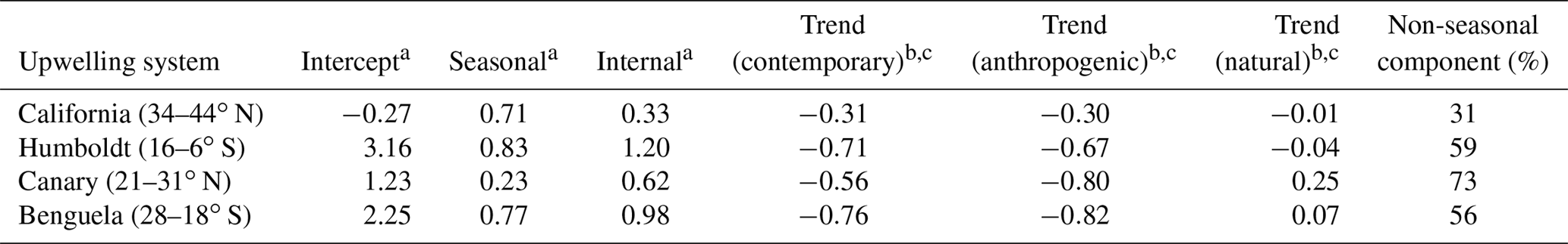
a mol m−2 yr−1; b mol m−2 yr−1 96 yr−1; c all trends are significant to α=0.05 for a one-sided Mann–Kendall test.
2.2 Upwelling regions and anomalies
Upwelling regions in each EBUS span approximately the 10∘ latitude of the most active upwelling, as defined by Chavez and Messié (2009); we shifted the CanCS upwelling domain north by 9∘ to capture the more intense upwelling off Western Sahara in CESM1 (Table 1). Following Turi et al. (2014), the EBUS upwelling regions span from the coastline to 800 km offshore, tracking the model coastline. The black outlines in Fig. 1e–h display these regions. The CESM-LENS ensemble mean incorporates the seasonal cycle and any long-term anthropogenic trends for a given variable. We therefore removed the ensemble mean from each simulation to create a time series of anomalies produced solely by internal climate variability. Note that for air–sea CO2 flux, these anomalies represent internal variability in the contemporary flux of CO2, or the combined variability of natural and anthropogenic CO2.
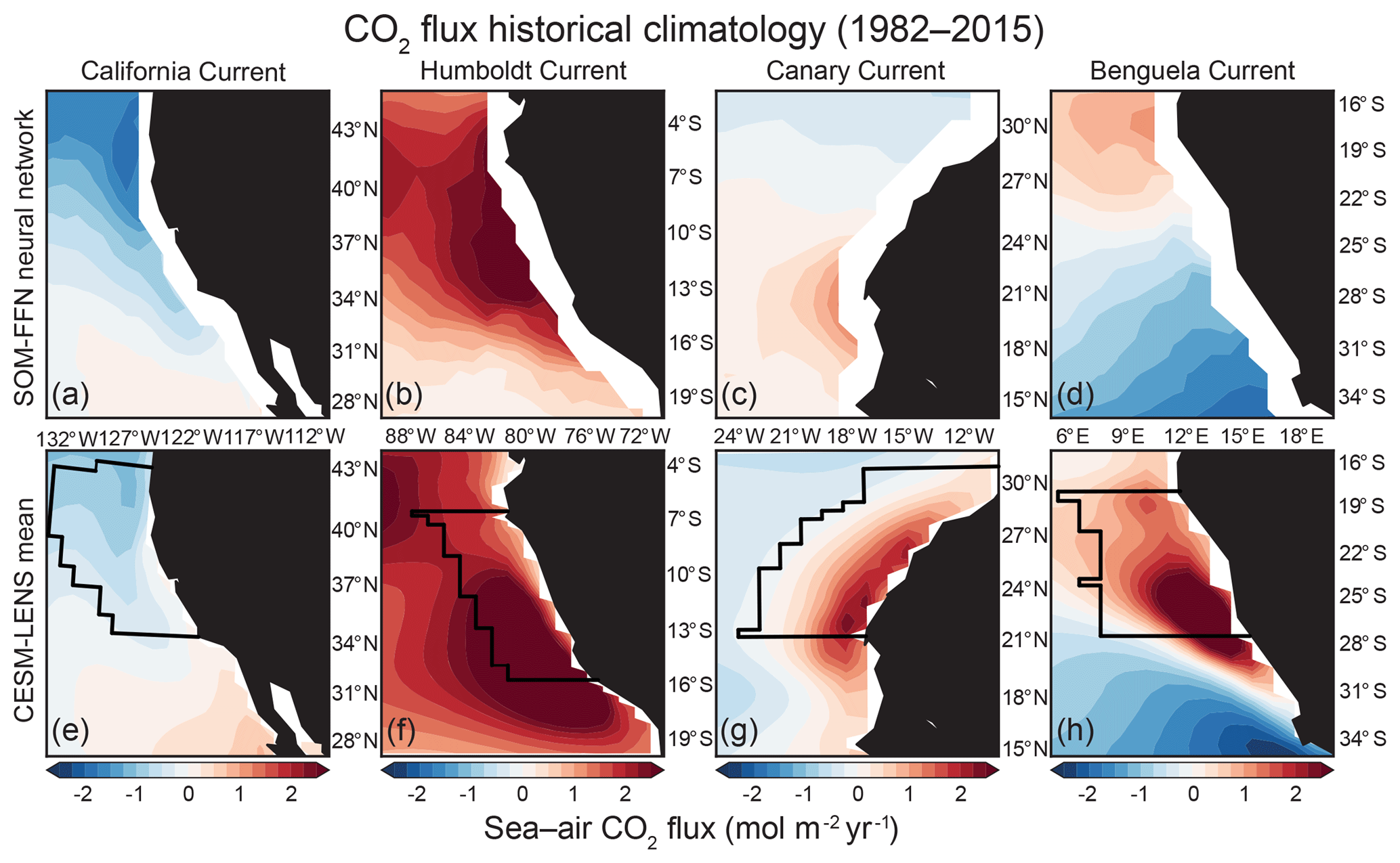
Figure 1Comparison of CO2 flux climatology from 1982–2015 between the SOM-FFN (a–d) and the CESM-LENS (e–h). Red denotes outgassing of CO2 from the ocean to the atmosphere, while blue represents uptake of CO2 by the ocean. Black lines in (e)–(h) follow the model grid and show the region used in each EBUS for statistical analysis, which is based on the 10∘ latitude of most active upwelling from Chavez and Messié (2009) and is confined to 800 km offshore in the E–W direction.
2.3 Climate indices
Throughout this paper, we regress anomaly time series of variables from each EBUS on climate indices. Climate index time series were available for each ensemble member for the PDO, NAO, Atlantic Multidecadal Oscillation (AMO), ENSO, and Atlantic meridional overturning circulation (AMOC) through the Climate Variability Diagnostics Package (CVDP; Phillips et al., 2014). We computed the NPGO index for each simulation following Di Lorenzo and Mantua (2016). These indices are available through the CESM-LENS project page (NPGO). Note that the NAO, NPGO, and PDO indices referred to in this study are based on normalized principal component time series and are thus reported in standard deviation (σ) units.
2.4 Model equations and statistical analyses
Air–sea CO2 fluxes in CESM are computed following the parameterization of Wanninkhof (2014):
where k represents the gas transfer velocity (dependent on the wind speed, U, squared), K0 is the solubility of CO2 in seawater, and and are the partial pressures of CO2 in the surface ocean and atmosphere, respectively.
We use a linear Taylor expansion to quantify the relative contribution of each variable to the overall air–sea CO2 flux anomaly in response to unforced variability following Lovenduski et al. (2007) and Turi et al. (2014),
where and are determined from the model equations and mean values in each EBUS. Δ's represent the linear regression of the given variable's anomalies onto a climate index. In addition to the linearization of the response, which results in us neglecting potentially important cross-derivative terms, we neglected further several terms in Eq. (2). In particular, we neglected the role of temperature and salinity for the solubility K0 and the gas transfer velocity k(U). This is justified, since the impact of salinity is small and the temperature sensitivity of the product k(U)⋅K0 is very small, owing to a strong cancellation effect. Furthermore we neglected the contribution of changes in atmospheric CO2, , primarily because these variations are at least 10 times smaller than those seen in surface ocean .
The contribution from is further decomposed into the contribution of changes in DIC, alkalinity (Alk), sea surface temperature (SST), and salinity,
The changes in DIC and Alk induced by freshwater fluxes have a strongly opposing influence on pCO2, thus it is often more instructive to separate this effect on DIC and Alk from the others and to summarize all salinity-related terms into a freshwater term (see Lovenduski et al., 2007, for details). The remaining, non-salinity-driven changes in DIC and Alk are referred to then as the salinity-normalized DIC (sDIC) and Alk (sAlk),
Due to the significance of sDIC anomaly contributions to the total CO2 flux anomaly in EBUSs, we approximate the mechanisms controlling sDIC anomalies following Lovenduski et al. (2007),
where , , and represent the sources and sinks of from circulation, biology, and CO2 flux anomalies integrated over the upper 100m, respectively. We refer the reader to Lovenduski et al. (2007, their Eq. 4) for additional details on these terms and to their Appendix B for the computation of in particular.
We use a Pearson product-moment correlation for all linear correlations performed in this study (e.g., between area-weighted CO2 flux anomalies and climate indices for each EBUS). Our null hypothesis is that the two time series being compared are uncorrelated, following the Student's t distribution with a significance level of α=0.05.
Autocorrelation is prevalent in climate indices such as the NPGO and ENSO (Di Lorenzo and Ohman, 2013), and our annual smoothing further enhances autocorrelation in CalCS and CanCS air–sea CO2 fluxes (see Sect. 3.3.1 and 3.3.3). To compensate for this autocorrelation, we replace the t-statistic sample size N with an effective sample size Neff, which quantifies the number of statistically independent measurements:
where r1 and r2 are the lag-1 autocorrelation coefficients of the two time series being correlated (Bretherton et al., 1999; Lovenduski and Gruber, 2005).
We use a one-sided Mann–Kendall test to assess significance in trends (e.g., the long-term diffusion of anthropogenic CO2 into EBUSs). Our null hypothesis is that the trend is not significantly different from zero, with α=0.05.
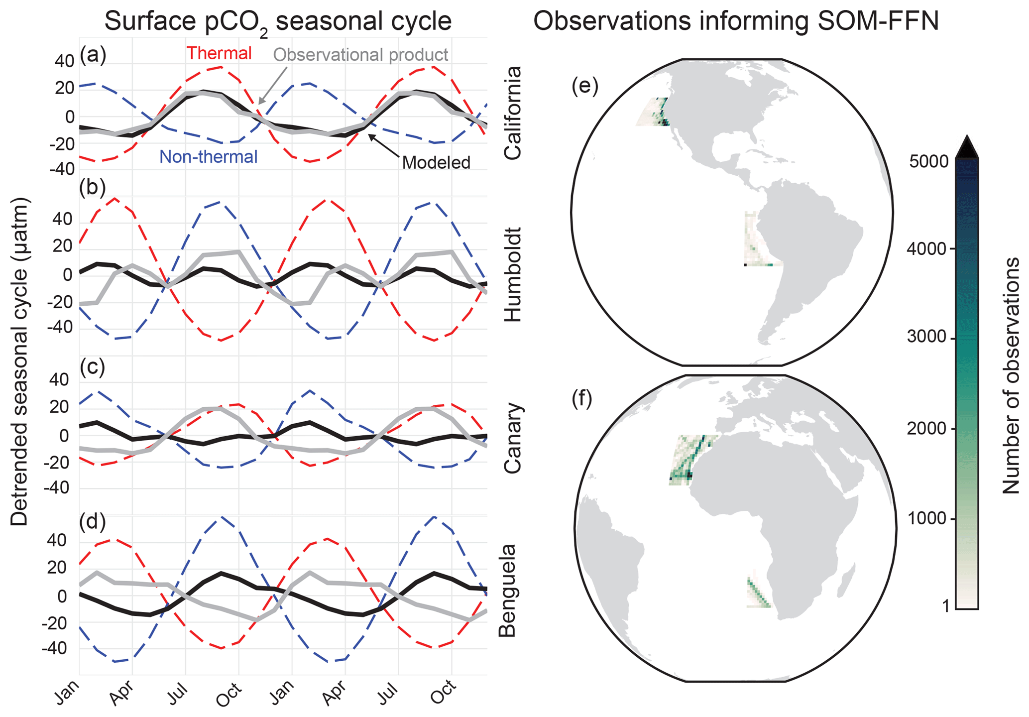
Figure 2Detrended surface pCO2 seasonal cycle from 1982–2015 for the SOM-FFN (gray) and the CESM-LENS ensemble mean (black) for the (a) CalCS, (b) HumCS, (c) CanCS, (d) and BenCS. Dashed red lines show the thermal component of the seasonal cycle for the CESM-LENS, and dashed blue lines show the non-thermal component. The total number of observations from SOCATv4 contributing to the SOM-FFN for the EBUSs is shown in (e) and (f).
3.1 Model evaluation
CESM-LENS air–sea CO2 flux climatologies and pCO2 seasonal cycles were compared to the SOM-FFN (self-organizing map – feed-forward network) product from Landschützer et al. (2017) along the four major EBUSs outlined by Chavez and Messié (2009). The SOM-FFN is a CO2 flux product based on numerous observational datasets and is made available at monthly resolution spanning 1982–2015 and at global resolution. Extensive details on and validation of the procedure can be found in Landschützer et al. (2013) and Landschützer et al. (2016). The SOM-FFN does not include coastal estimates, which presumably would have stronger outgassing due to coastal and curl-driven upwelling of DIC-enriched waters. Another important caveat is that the average number of pCO2 observations in EBUSs informing the SOM-FFN (637, 119, 517, and 195 for the CalCS, HumCS, CanCS, and BenCS, respectively) is on the order of the Southern Ocean (536), a notably under-sampled region (Fig. 2e and f; Bakker et al., 2016). An extension of the SOM-FFN approach to the coastal ocean by Laruelle et al. (2017) demonstrated that the coastal pCO2 values are not substantially different from the offshore, so the conclusions drawn from the open ocean Landschützer product still hold.
3.1.1 Air–sea CO2 flux climatology
The mean state of Pacific EBUS CO2 fluxes is particularly well modeled in the CESM-LENS (Fig. 1). The CESM-LENS captures the meridional gradient of poleward uptake and equatorward outgassing of CO2 in the CalCS (Fig. 1e). In the HumCS, the model depicts the strong outgassing that is characteristic of a tropical upwelling system (Fig. 1f). The CO2 flux climatology in the Atlantic systems is more biased in the CESM-LENS, with a tendency for spurious or stronger outgassing than that suggested by the observational product. While the SOM-FFN portrays a meridional gradient of relatively weak CO2 fluxes in the CanCS, the CESM-LENS simulates strong outgassing along Western Sahara (Fig. 1c and g). The BenCS has the most biased CO2 flux climatology of the major EBUSs in the CESM-LENS. Although it simulates the proper meridional gradient, the outgassing cell is nearly 10∘ too far south and is significantly stronger than in the SOM-FFN (Fig. 1d and h).
The BenCS has larger physical biases in the CESM-LENS than all other EBUSs. Its SST bias is in excess of 7 ∘C with the nominal 1∘ atmospheric resolution, compared to less than a 1 ∘C bias in the CalCS and CanCS and a 1–3 ∘C bias in the HumCS (R. Justin Small, personal communication, 2018). This bias is likely driven by the fact that the Angola–Benguela front is simulated too far south, in addition to deficiencies in upwelling and meridional transport that are caused by unrealistic alongshore wind stress structure (Small et al., 2015). Because these deficiencies are specific to the BenCS, we will only discuss its representation of the pCO2 seasonal cycle in Sect. 3.1.2, and its internal variability in CO2 fluxes in Sect. 3.2, but will not perform a full analysis on its connections to larger-scale climate variability.
3.1.2 pCO2 seasonal cycle
CESM-LENS simulates the pCO2 seasonal cycle well for the Pacific EBUSs, with larger error in the Atlantic EBUSs. In the CalCS, the CESM-LENS nearly perfectly matches the SOM-FFN in both amplitude and phase (Fig. 2a). The system exhibits its maximum pCO2 (and thus CO2 outgassing) in August and its minimum pCO2 (and thus CO2 uptake) in April. We further decomposed the model seasonal cycle into its thermal component (driven by the seasonality of SST) and its non-thermal component (driven by the seasonality of factors such as DIC, Alk, and salinity) following Takahashi et al. (2002). This decomposition suggests that the phase of the CalCS seasonal cycle is determined by thermal (solubility) effects, with its amplitude modulated by non-thermal factors (Fig. 2a). These non-thermal factors are almost entirely driven by the seasonal cycle of DIC (not shown), which is characterized by photosynthetic uptake of CO2 in the summer and fall, coinciding with upwelling season. In the HumCS, both the CESM-LENS and SOM-FFN suggest a dual peak in the seasonal cycle of pCO2, although the model and observational product slightly disagree in phase and amplitude (Fig. 2b). These two peaks are driven by an alternating dominance of thermal and non-thermal effects.
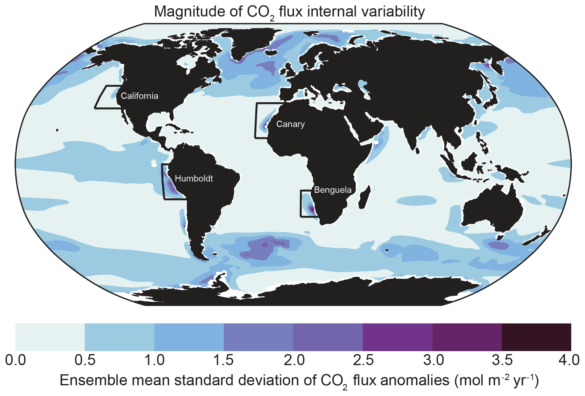
Figure 3Magnitude of internal variability in CO2 flux from 1920–2015 in the CESM-LENS. Anomalies were generated by removing the ensemble mean – which represents the seasonality and forced signal – from each realization. Internal variability was then quantified by taking the ensemble mean standard deviation of the anomalies from 1920–2015. Here, the black boxes outline the general domain of the EBUSs in this study but do not coincide with the statistical boundaries shown in Fig. 1.
During the austral summer and fall, warm temperatures lead to enhanced pCO2 that is slightly compensated for by increased biological activity, similar to the singular peak of the CalCS. In the austral winter and spring, intense upwelling of DIC-enriched waters and reduced biological activity that is slightly compensated for by cooler waters leads to a secondary pCO2 peak (Kämpf and Chapman, 2016). The SOM-FFN suggests that the CanCS behaves similarly to the CalCS, with a single pCO2 peak in late summer and fall that is in phase with the seasonal cycle of SST (Fig. 2c). However, the CESM-LENS simulates a damped seasonal cycle that is approximately 180∘ out of phase for pCO2 in the CanCS that results from a delicate balance between thermal and non-thermal effects of similar magnitudes. Despite the thermal and non-thermal effects being in the proper phase for a system of the Northern Hemisphere, the SST seasonal cycle is too weak and the DIC seasonal cycle too strong in the CanCS in the CESM-LENS. Lastly, we find that the CESM-LENS simulates the BenCS pCO2 seasonal cycle nearly 180∘ out of phase with the SOM-FFN representation (Fig. 2d). Similar to the CanCS, the thermal and non-thermal effects are in the proper phase. However, there is a large bias in the magnitude of the DIC seasonal cycle, which overwhelms the thermal seasonality and drives the pCO2 seasonal cycle entirely out of phase.
3.2 Internal variability in upwelling systems
We emphasize the magnitude of internal variability in EBUS air–sea CO2 fluxes in Fig. 3 by showing the ensemble mean standard deviation of air–sea CO2 flux anomalies (ensemble mean subtracted) at each location across the global ocean. Save for the Southern Ocean and subpolar Arctic, the EBUSs emerge as regions of high internal variability on a global scale. The HumCS, CanCS, and BenCS in particular have some of the highest unforced variability in CO2 fluxes globally. The CalCS has comparatively low internal variability in CO2 fluxes. The EBUSs generally have higher internal variability than other coastal regions and are particularly distinct from the major western boundary currents, which appear to be influenced very little by internal variability (Fig. 3). The internal variability can also be isolated as one constituent of the area-weighted CO2 flux time series for each of the four EBUSs, the others being the forced trend and seasonal cycle (Fig. 4a–d). The largest absolute internal variability component of the standard deviation of CO2 flux is found in the BenCS (0.98 mol m−2 yr−1) and the HumCS (1.20 mol m−2 yr−1; Table 1). The BenCS is uniquely exposed to variability from the Southern Ocean and Agulhas Current (Reason et al., 2006). The HumCS likely has intense variability due to its proximity to the tropical Pacific Ocean and thus rapid communication with ENSO (e.g., Colas et al., 2008; Montes et al., 2011).
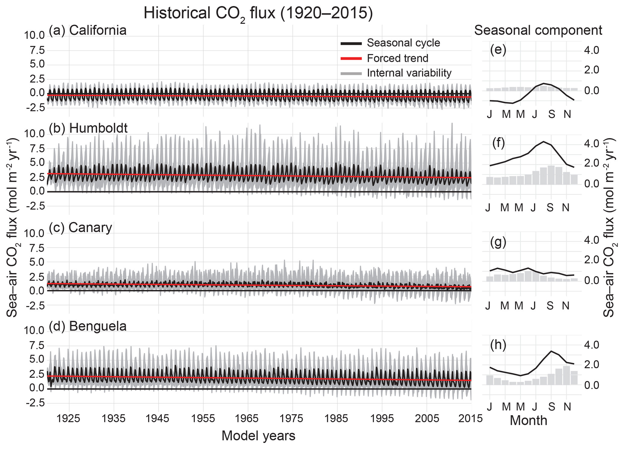
Figure 4Time series of historical CO2 flux (1920–2015) in the CESM-LENS for each of the four studied upwelling systems (a–d). The ensemble mean yields both the seasonal cycle (black) and the forced trend (red). Gray shading shows the bounds of the maximum and minimum realizations due to internal variability, but also contains signal from the seasonal cycle and forced trend. Table 1 displays the intercept, seasonality, internal variability, and forced trend for each system. (e)–(h) show the mean seasonal cycle (black line) and ensemble mean monthly internal variability (gray bars) for 1920–2015 for each system.
All four systems have statistically significant trends toward a weaker CO2 source or greater CO2 sink over 1920–2015, due mainly to the invasion of anthropogenic carbon from the atmosphere (Fig. 4; Table 1). Note that in the CanCS and BenCS, there is a trend toward more outgassing of natural CO2, which is compensated for by the relatively large uptake tendency of anthropogenic CO2 (Table 1). The long-term trend forces the HumCS, CanCS, and BenCS to act as intermittent seasonal sinks by 2015 in some realizations, due to the combination of the long-term trend and internal variability (Fig. 4). The BenCS and CanCS have the largest uptake of anthropogenic CO2 over the historical period, although the HumCS has a relatively large uptake of both natural and anthropogenic CO2 (Table 1). For the HumCS and BenCS, the contemporary CO2 flux trend is on the order of the magnitude of their seasonal cycles over the course of 96 years. The CanCS is a unique case, where the contemporary trend is more than double the magnitude of its seasonal cycle (Table 1).
The magnitude of internal variability in the combined natural and anthropogenic CO2 fluxes is greater than that of the seasonal cycle for the majority of systems. The non-seasonal component of the total variability (the sum of the seasonal and internal components) is 59 % for the HumCS, 73 % for the CanCS, and 56 % for the BenCS (Table 1). Only the CalCS has a stronger seasonal cycle of CO2 flux than internal variability, but the non-seasonal component still accounts for 33 % of the total variability in this system (Table 1). Lastly, internal variability in CO2 fluxes tends to be phase locked with the seasonal cycle, as the peak magnitudes of internal variability track the ridges and troughs of the seasonal component (Fig. 4).
3.3 Climate variability and air–sea CO2 fluxes
Our primary goal for each EBUS was to identify the mode of climate variability most strongly associated with its CO2 flux anomalies. We correlated area-weighted anomalies from the black boxes in Fig. 1e–h for each simulation with every grid cell globally for a set of predictor variable anomalies: SST, sea level pressure (SLP), 10 m wind speed, and wind stress curl. We then assessed the ensemble mean of the correlations to determine the mode of climate variability associated with the given global spatial pattern. Figure 5 displays one ensemble mean correlation case for the CalCS (panel a), HumCS (panel b), and CanCS (panel c) as well as violin plots showing the spread of correlations across the 34-member ensemble for Pacific (Fig. 5d–e) and Atlantic (Fig. 5f) modes of variability.
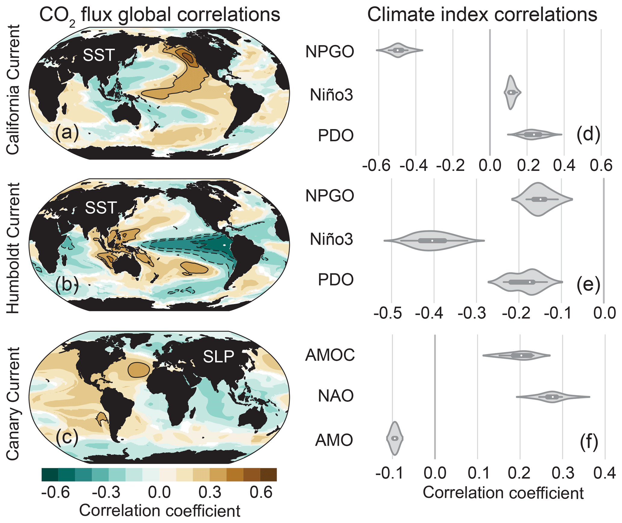
Figure 5Correlations between area-weighted CO2 flux anomalies in the statistical study regions outlined in black in Fig. 1 (e–g) and SSTa (a–b; California, Humboldt) and SLPa (c; Canary) grid cells globally. Brown colors indicate that positive SSTa and/or SLPa correlates with outgassing, and blue with uptake. Contour lines begin at ±0.3 and progress in intervals of 0.1. Correlations were performed for each realization individually, and the ensemble mean of those global correlations are presented here. Violin plots display correlations between area-weighted CO2 flux anomalies from (a) to (c), with major modes of Pacific (d–e) and Atlantic (f) variability. The interior of the violin plot displays a box plot with the ensemble mean denoted as a white dot. Shading around the box plot reflects the ensemble distribution of correlations, which are mirrored on either side.
3.3.1 California Current
The correlation between CalCS CO2 flux anomalies and SST anomalies (SSTa's) yields a map suggestive of Pacific decadal variability, due to the zonal dipole of correlations in the North Pacific (Fig. 5a; Mantua and Hare, 2002; Di Lorenzo et al., 2008). Although similar in structure to the PDO, this map most closely resembles the NPGO (Di Lorenzo et al., 2008). In fact, correlations between the model-based NPGO with annual smoothing and CalCS CO2 flux yields a correlation coefficient of . In comparison, linear correlations with the PDO result in a correlation coefficient of 0.24±0.05 (Fig. 5d). Thus, we highlight the NPGO as the major mode of climate variability associated with anomalous CO2 flux in the CalCS.
Table 2Estimated contributions of individual terms to air–sea CO2 flux anomalies, ΔF, in response to a mode of climate variability using Eq. (4). Each row under “Individual terms” depicts the ensemble mean contribution and ensemble spread for Figs. 6–9. The column “CalCS–PDOn” reflects results from the nearshore box in the CalCS in Fig. 7, and “CalCS–PDOo” reflects results from the offshore box. Σ is the sum of all contributing first-order terms (i.e., all rows under “Individual terms” or the right-hand side of Eq. 4). ΔF is the direct regression of CO2 flux anomalies on the specified mode of climate variability (i.e., the left-hand side of Eq. 4).

a mol m−2 yr−1 σ−1; b mol m−2 yr−1 K−1.
We find that the CalCS has a single-signed response to the NPGO with anomalous uptake of CO2 during a positive event, intensifying the mean state of the system as an uptake site (Fig. 6). The direct regression of ΔF onto the NPGO results in an anomalous uptake of 0.10 mol m−2 yr−1 σ−1 (where “σ” refers to one standard deviation of the normalized principal component time series for the NPGO; Table 2), which is roughly 24 % of the long-term historical CO2 flux mean of −0.42 mol m−2 yr−1. The primary contributions to this uptake anomaly come from variations in SST and sDIC, which are mainly driven by changes to offshore gyre dynamics. As the oceanic expression of the North Pacific Oscillation, the NPGO is associated with intensified geostrophic circulation, resulting in increased transport in both the California Current and the Alaska Coastal Current (Di Lorenzo et al., 2008). Furthermore, a positive NPGO leads to enhanced upwelling-favorable winds south of Cape Mendocino (Fig. S1). During the positive NPGO phase, the entire CalCS cools, increasing the CO2 solubility (Fig. 6; Fig. S1). Although downwelling is enhanced offshore, increased DIC transport from the Alaskan Gyre leads to a tendency for outgassing of CO2 (Fig. S1). Near the shore south of Cape Mendocino, increased upwelling of DIC-enriched waters is compensated for by photosynthesis, leading to near-zero CO2 flux anomalies (Fig. S2). North of Cape Mendocino, weakened upwelling and low subsurface DIC anomalies lead to enhanced uptake anomalies (Figs. S1 and S2). Because the system-wide contributions of SST and sDIC to the anomalous flux nearly balance each other out, minor contributions from wind, salinity, sAlk, and freshwater flux push the system in favor of anomalous uptake (Fig. 6).
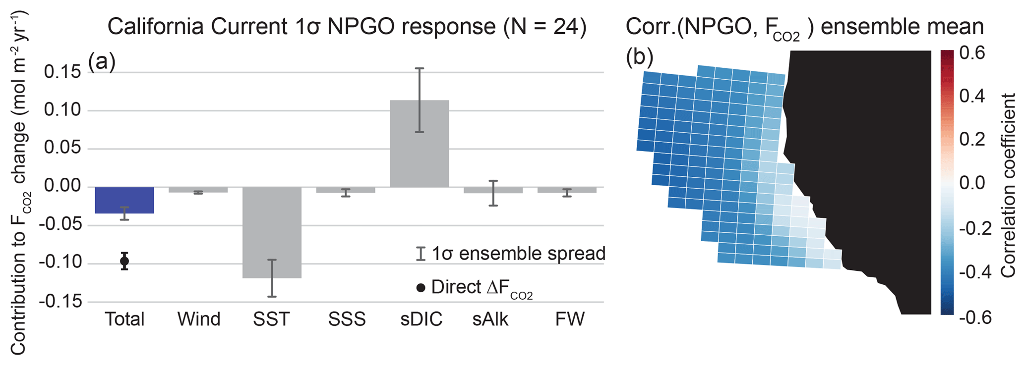
Figure 6Linear Taylor expansion from Eq. (4) for CalCS CO2 flux anomalies regressed on the NPGO (a). Gray bars represent the ensemble mean contributions of each variable to the CO2 flux anomaly. Error bars represent the 1-standard-deviation spread of the full ensemble. The individual bars sum to the “total” bar to approximate the direct regression of on the NPGO, which is denoted as the black dot with its associated ensemble spread. The ensemble mean grid cell correlations between CO2 flux anomalies and the NPGO in the CalCS study region are displayed in (b). Positive correlations are associated with outgassing; negative correlations are associated with uptake. The magnitude and ensemble spread for each bar is presented in Table 2.
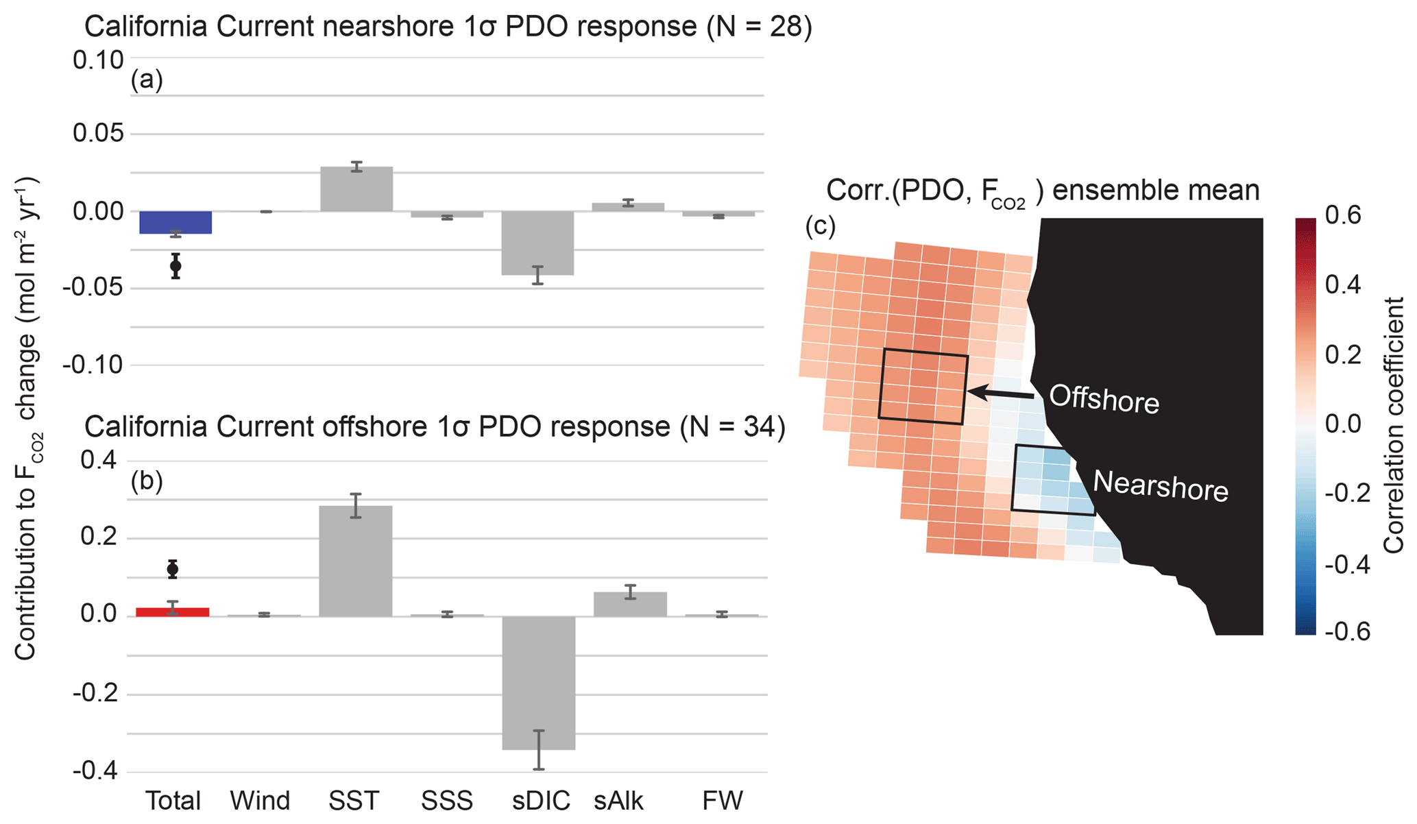
Figure 7As in Fig. 6, but in response to the PDO for a nearshore region (a) and offshore region (b). Note that the offshore decomposition (b) has a y-axis range 4 times that of the nearshore decomposition (a).
The CalCS has the largest relative ensemble spread in sDIC and sAlk (Fig. 6; Table 2). This is potentially because of inter-simulation variability in the response of CalCS dynamics to the NPGO due to atmospheric noise (as in the case of ENSO in Deser et al., 2017, 2018), which can directly alter the biogeochemical properties of source waters that feed the region (Pozo Buil and Di Lorenzo, 2017). Although the linear Taylor expansion approximates a CO2 flux anomaly nearly half that of the direct regression of ΔF onto the NPGO, it is still of the same sign. This discrepancy is due to the influence of higher-order and cross-derivative terms that we did not account for in our linear approximation.
We also performed this analysis for the CalCS response to a 1σ positive (warm) phase of the PDO (Fig. 7a and b). Every ensemble member displayed a dipole response to the PDO (not shown), with anomalous uptake in the nearshore region south of Cape Mendocino and anomalous outgassing elsewhere in the domain (Fig. 7c). This was the only case in which we found a non-single-signed response across all ensemble members to any mode of climate variability investigated. However, note that the dipole pattern is quite similar to that of the CalCS response to the NPGO (Fig. 6b). Both the nearshore and offshore regions have modest correlations with the PDO, with correlation coefficients of and 0.28±0.05, respectively. The positive phase of the PDO results in anomalously warm SSTs along the CalCS and causes weaker and shallower upwelling cells with higher retention of nutrient- and carbon-depleted surface waters (Fig. S3; Chhak and Di Lorenzo, 2007). This aligns with the inverted contributions of SST and sDIC in Fig. 7a and b, relative to the contributions of these terms in response to the NPGO (Fig. 6a). The warming of CalCS SSTs during a positive phase of PDO causes a reduction of CO2 solubility and thus a tendency toward outgassing (Fig. 7). Anomalous poleward coastal winds associated with the positive phase of the PDO result in reduced coastal and curl-driven upwelling along the entire coastline and weakened curl-driven downwelling offshore (Fig. S3). In coordination with reduced subsurface DIC throughout the region, these changes in circulation contribute toward anomalous uptake of CO2 throughout the CalCS. Note that the nearshore decomposition in Fig. 7a has a y-axis range 4 times smaller than that of the offshore decomposition. This slight uptake anomaly is the result of a delicate balance of minor terms, where the sDIC reduction slightly outweighs the warming effect. On the other hand, the offshore region has contributions from SST and sDIC that are as much as triple the magnitude of that for the NPGO (Table 2). Despite the sDIC reduction being larger than the SST term, the reduced sAlk is substantial enough to cause a slight outgassing anomaly offshore (Fig. 7b).
The direct response of winds to the NPGO and PDO plays a negligible role in influencing anomalous CO2 flux in the CalCS (Table 2). Although the ΔU in response to the NPGO and PDO is on the order of the HumCS and CanCS, is 3–10 times smaller than the other systems. is based on the climatological mean U, ΔpCO2, and Schmidt number. The CalCS has the smallest mean ΔpCO2 of the EBUSs, at just 0.2 µatm. This causes CO2 flux in the system to be relatively insensitive to fluctuations in the wind.
3.3.2 Humboldt Current
Global correlations between the HumCS CO2 flux anomalies and SSTa display ENSO as a major influence, with regions of high correlation focused around the equatorial Pacific (Fig. 5b). Correlations between HumCS CO2 flux anomalies and the Niño3 index resulted in a correlation coefficient of (Fig. 5e). Similar results were found for the Niño3.4 index () and the Niño4 index (). We chose the Niño3 index as our primary predictor of HumCS CO2 flux anomalies, since it is more eastern focused and thus captures the stronger spatial correlations closest to the HumCS (Fig. 5b).
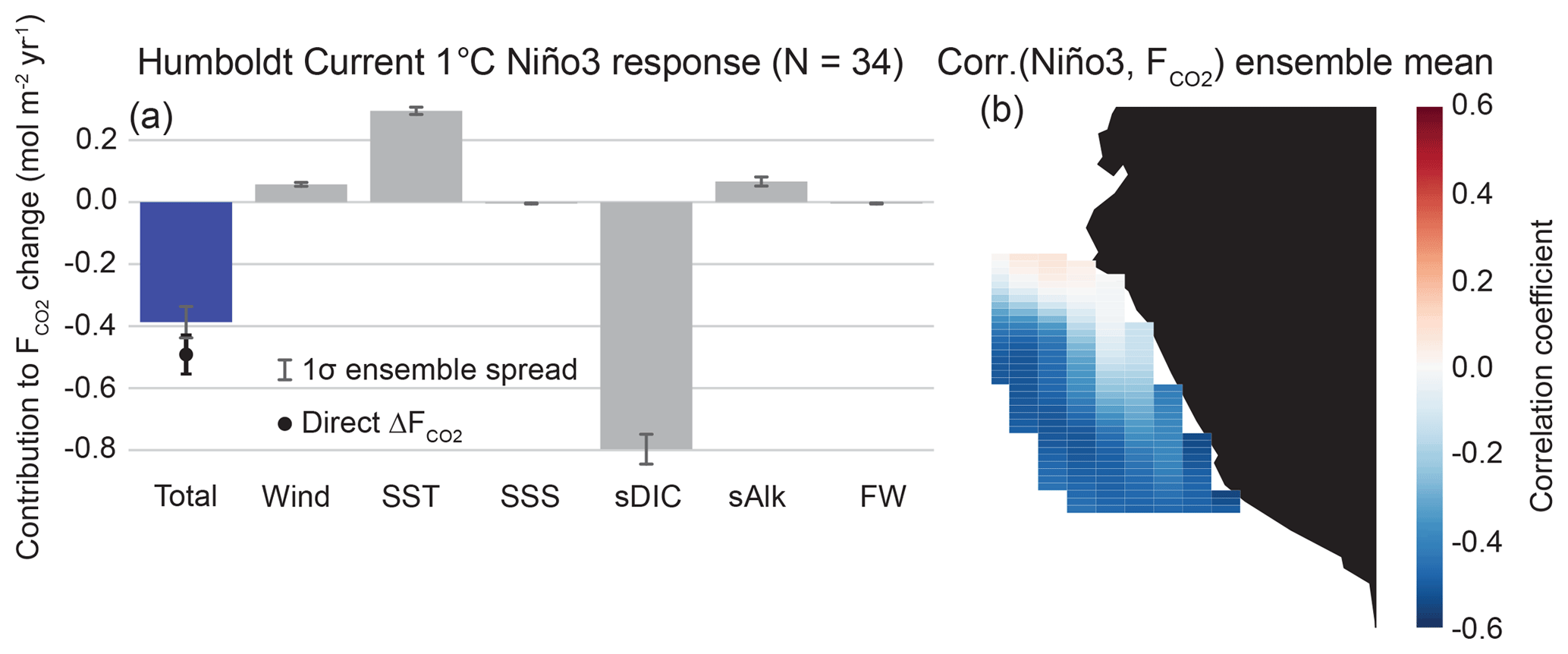
We present the results of a linear Taylor expansion for HumCS CO2 flux anomalies regressed onto a 1 ∘C El Niño in Fig. 8 (Eq. 4). We find that the HumCS responds with a nearly single-signed CO2 uptake anomaly, resulting in a weakening of the climatological outgassing (Fig. 8b). Although there is a small region in the northern HumCS that responds with an outgassing anomaly, it not nearly as coherent across the ensemble as the spatial dipole response of the CalCS to the PDO (Fig. 7c). The direct regression of ΔF onto the Niño3 index results in an anomalous uptake of 0.49 mol m−2 yr−1 K−1, which is approximately 18 % of the long-term historical CO2 flux mean of 2.8 mol m−2 yr−1. As in the case of the CalCS, the two major terms contributing to the uptake anomaly are sDIC and SST, which are of the opposite sign (Fig. 8a). We would anticipate this to be the case, as an El Niño event induces warming along the HumCS and reduces the efficacy of upwelling for bringing carbon- and nutrient-rich waters to the surface due to the presence of an anomalously deep thermocline (Fig. S4; Strub et al., 1998). While upwelling-favorable winds tend to decrease along Chile (outside of our study region) during an El Niño event, the coastal wind response along Peru is variable, ranging anywhere from slight downwelling-favorable to slight upwelling-favorable anomalies (Wyrtki, 1975; Enfield, 1981; Huyer et al., 1987).
In the CESM-LENS, the HumCS experiences a warming of 0.7 ∘C for a 1 ∘C El Niño, which results in an outgassing tendency of 0.3 mol m−2 yr−1 K−1 (Table 2). However, sDIC in the system is reduced by 13.2 mmol m−3 K−1 for the same event, which translates to a large uptake contribution of 0.8 mol m−2 yr−1 K−1 (Table 2). This is an enormous change in sDIC, which is partially driven by the high subsurface DIC bias in the eastern equatorial Pacific in CESM1 (see Lovenduski et al., 2015, their Fig. 2). The large sDIC reduction is due to weakened upwelling and a deepening of the thermocline by warm water advected from the equatorial Pacific (Fig. S4). Although the passage of coastally trapped waves are important in the HumCS, they are not resolved in the coarse-resolution CESM-LENS. Lastly, there is a minor outgassing anomaly of 0.06 mol m−2 yr−1 K−1 in response to a slight increase in wind speed during El Niño (Table 2). Despite the significant contributions of wind speed, SST, and sAlk toward outgassing, the large reduction in sDIC drives an uptake anomaly that weakens the HumCS outgassing during an El Niño event. Note that these are the same mechanisms that are responsible for reduced outgassing in the tropical belt in response to an El Niño (Feely et al., 1999).
3.3.3 Canary Current
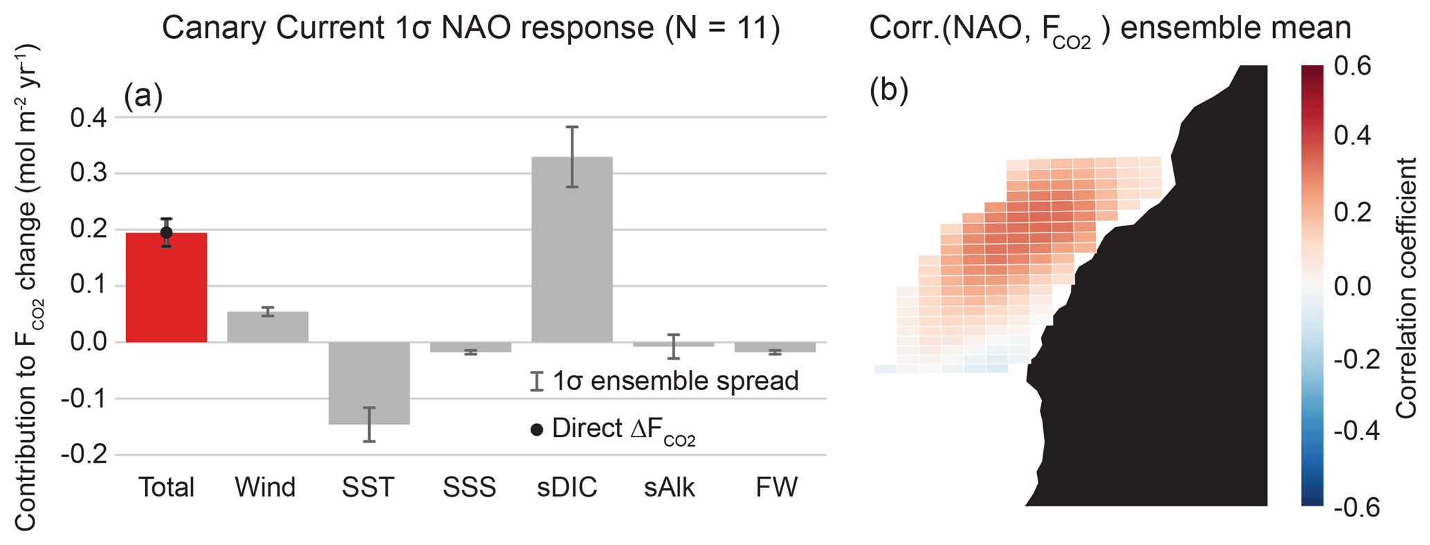
Correlations between the CanCS CO2 flux anomalies and SLP anomalies (SLPa's) globally reveal a region of high positive correlation coefficients just northwest of Africa. This coincides with the climatological position of the Azores High, the large-scale anticyclone which forces the CanCS. The climate index that most directly captures variability in the Azores High is the NAO and will thus be considered the main mode of climate variability that modulates anomalous CO2 flux in the CanCS. We find modest correlations of 0.28±0.03 between annually smoothed CanCS CO2 flux anomalies and the NAO (Fig. 5f). Relatively lower correlations are expected between anomalous EBUS CO2 fluxes and atmospheric indices, as the atmosphere is noisier than the more slowly evolving ocean.
Grid cell correlations between CanCS CO2 flux anomalies and the NAO are displayed in Fig. 9b. The CanCS has a nearly single-signed response of increased outgassing during the positive phase of the NAO. The direct regression of ΔF onto a 1σ NAO results in an outgassing anomaly of 0.2 mol m−2 yr−1 σ−1 (Table 2), which is 21 % of the historical CO2 flux mean of 0.95 mol m−2 yr−1. As with the other EBUSs, the major contributors toward this anomaly are sDIC and SST (Fig. 9a). The NAO represents fluctuations in the intensity of atmospheric circulation between the Azores High and Icelandic Low (Hurrell et al., 2001). During the positive phase of the NAO, a stronger Azores High leads to intensified alongshore winds and thus more vigorous upwelling (Fig. S5). This brings up additional deep cold water, which in turn increases the CO2 solubility of the system, tending toward an uptake anomaly of 0.15 mol m−2 yr−1 σ−1 (Table 2). On the other hand, the increased sDIC from intensified upwelling is double the magnitude of the SST contribution, despite the increased biological activity which reduces some of the physical sDIC input, leading to an outgassing anomaly of 0.33 mol m−2 yr−1 σ−1. This large sDIC response is driven both by a high ΔsDIC of 3.9 mmol m−3 σ−1 as well as by the fact that the CanCS has the highest of the major EBUSs. Increased winds of 0.3 m s−1 σ−1 lead to a significant outgassing pressure of 0.05 mol m−2 yr−1 σ−1. This is due to both a large system sensitivity, , to changes in wind and a high wind anomaly in response to the NAO. Ultimately, intensified winds and an anomalous increase in sDIC due to enhanced upwelling counteracts the solubility effects of colder SSTs and increased photosynthetic uptake of sDIC.
We find that the seasonal cycle of pCO2 is single peaked, and its phase is driven by thermal (solubility) effects in the CalCS, CanCS, and BenCS, while non-thermal effects modulate its amplitude. The seasonal cycle of pCO2 in the HumCS is dual peaked and driven by an alternating dominance of thermal and non-thermal effects. Although the CESM-LENS models the CalCS and HumCS pCO2 seasonal cycle well, the CanCS seasonal cycle is damped, and both the CanCS and BenCS seasonal cycles are nearly 180∘ out of phase (Fig. 2).
Variations in sDIC and SST in response to large modes of climate variability exert the most influence on anomalous CO2 fluxes in the CalCS, CanCS, and HumCS. Furthermore, these terms always act in opposition to one another in the portions of variability associated with the climate indices explored in this study. Secondary to these terms are wind speed and sAlk. Although their contributions do not rival those of SST and sDIC in magnitude, they act to further reinforce anomalies or to tip the balance toward outgassing or uptake when the terms associated with SST and sDIC are of about equal magnitude. In all systems, salinity and freshwater fluxes have negligible contributions toward the total CO2 flux anomaly.
CalCS and CanCS CO2 flux anomalies are associated mainly with climate modes related to large-scale anticyclones, with their mean states (uptake for the CalCS and outgassing for the CanCS) intensified during phases of enhanced gyre circulation in the NPGO and NAO, respectively. CO2 flux anomalies in the HumCS are mostly driven by ENSO, due to its close proximity to the equatorial Pacific. We find that the HumCS has weakened outgassing during El Niño due to reduced upwelling and a deepening of the thermocline, which are similar mechanisms to the equatorial Pacific's response to El Niño (Feely et al., 1999).
Table 3Regression coefficients between the given EBUS and climate index for anomaly time series of the estimated contributions toward the sDIC tendency integrated over the upper 100 m and the total surface area of the system, as in Eq. (5).

a Tg C yr−1 σ−1; b Tg C yr−1 K−1
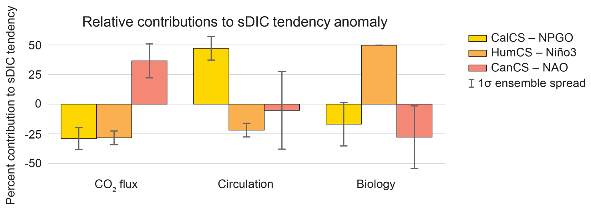
Figure 10Relative contributions of anomalous air–sea CO2 flux, physical circulation, and biology to the approximated sDIC tendency anomaly for the CalCS (yellow), HumCS (orange), and CanCS (red) in response to the NPGO, Niño3, and NAO, respectively. Error bars show the 1-standard-deviation spread of the ensemble. For a given simulation, the absolute magnitude of the three components sum to 100 %. These values were approximated using Eq. (5).
Because sDIC anomalies are so critical to the EBUS response to internal climate variability, we further decomposed these anomalies into their absolute (Table 3) and relative (Fig. 10) contributions from circulation (e.g., upwelling, advection, and mixing), biology (photosynthesis, respiration, and calcium carbonate formation and dissolution), and air–sea CO2 fluxes. Changes in biological activity in the HumCS in response to ENSO contribute to nearly 50 % (8.61 Tg C yr−1 K−1) of the total sDIC tendency anomaly (Fig. 10, Table 3). During an El Niño enhanced respiration pumps sDIC into the upper water column, while photosynthesis removes sDIC during a La Niña. While biology is the major contributor to sDIC tendency anomalies in the HumCS, circulation changes play a leading role in the CalCS. In response to the NPGO, circulation anomalies in the CalCS contribute roughly 47 % (1.47 Tg C yr−1 σ−1) of the total sDIC tendency anomaly (Fig. 10; Table 3). It is difficult to assess the relative contributions of and in the CanCS, as the large ensemble spread in drives a highly uncertain , which is computed as the anomaly of the other three terms (Fig. 10). In all three systems, CO2 flux anomalies play an important role in modifying the sDIC tendency, with an ensemble mean relative contribution greater than 25 % (Fig. 10). Note, however, that significant spatial variability exists for circulation and biology contributions in the HumCS, and moderate spatial variability exists in the CanCS. In contrast, contributions are relatively uniform throughout the CalCS (Fig. S7).
It is important to note that anthropogenic climate change will likely modify our findings over the coming decades in a number of ways. The long-term addition of anthropogenic carbon to the surface ocean causes EBUSs to become greater sinks for CO2. This trend shifts the mean state of the EBUSs, causing historical outgassing sites (the HumCS, CanCS, and BenCS) to become intermittent net sinks of CO2 under the influence of internal variability by the end of the historical period (Fig. 4). Projecting to 2100 under RCP8.5 forcing, we find that the CanCS and BenCS become net sinks for CO2 due to the anthropogenic trend, with mean CO2 uptake of −0.43 and −0.04 mol m−2 yr−1 over 2016–2100, respectively. The addition of anthropogenic CO2 into the surface ocean can also intensify the magnitude of the seasonal cycle of CO2 flux. This is due to the increased concentration of CO2 in the surface ocean as well as the reduction in the ocean's buffer capacity, which makes pCO2 more sensitive to seasonal fluctuations in DIC and alkalinity (Landschützer et al., 2018, and references therein). This effect has been shown in observations (Landschützer et al., 2018) and is also projected in climate models (Kwiatkowski and Orr, 2018), but is only seen significantly in the CalCS and CanCS in the CESM-LENS, with an approximate 37 % and 30 % increase in the CO2 flux seasonal cycle over 2016–2100, respectively. Negligible changes to the seasonal cycle over the next century are projected for the HumCS and BenCS in the CESM-LENS.
External forcing will also alter the dynamics of the EBUSs (Bakun et al., 2015; García-Reyes et al., 2015), potentially inducing changes to alongshore winds (Narayan et al., 2010; Sydeman et al., 2014; Oerder et al., 2015; Rykaczewski et al., 2015; Wang et al., 2015) and upper-ocean stratification (Di Lorenzo et al., 2005; Rykaczewski and Dunne, 2010; Oerder et al., 2015), which will in turn influence the rate and efficacy of upwelling. It is unlikely that changes to vertical transport will be detectable until mid-century, as the anthropogenic signal is obscured by internal variability (Brady et al., 2017). However, externally forced trends in stratification are likely to emerge much quicker (Henson et al., 2016). The biogeochemical signature of waters feeding upwelling (e.g., O2, CO2, and nutrient concentrations) will likely also be modified due to these dynamical changes as well as to changes to ocean ventilation and source water pathways (Rykaczewski and Dunne, 2010). Externally forced changes in physical and biogeochemical properties of EBUSs will likely alter the relative contributions of different physical processes to anomalous CO2 fluxes, as approximated by Eq. (4) and shown in Figs. 6–9 and Table 2. It is also possible that modes of climate variability will change in response to anthropogenic forcing. Model projections and long-term observations have suggested that the intensity, frequency, or variance associated with ENSO (e.g., Timmermann et al., 1999; Cai et al., 2014, 2015), the NAO (Kuzmina et al., 2005), and the NPGO (Sydeman et al., 2013) has changed significantly in recent decades or will change over the next century. These modifications to modes of climate variability suggested by the literature could directly impact the response of EBUS CO2 flux anomalies to internal variability, thus affecting the conclusions of our study. Further investigation of the impacts of anthropogenic climate change on CO2 fluxes in EBUSs is necessary for the community.
This study serves as a starting point toward better understanding how internal climate variability modulates CO2 fluxes in the major EBUSs. We present the mode of climate variability that has the largest influence on anomalous CO2 fluxes in the HumCS and CanCS and the leading two modes for the CalCS. Because of this, we account for approximately 16 % of the total CO2 flux variance in the HumCS and 8 % in the CanCS. Since we analyzed statistically orthogonal modes (the PDO and NPGO) in the CalCS, we account for as much as 31 % of the total CO2 flux variance. It is difficult to explain a large chunk of the remaining variance for the EBUSs, as other modes of internal variability are physically dependent on one another. Furthermore, locally generated atmospheric noise in the EBUSs can contribute substantially to the total modeled CO2 flux variance. Previous studies that relate anomalous CO2 fluxes to internal climate variability have explained similar amounts of variance. For example, Lovenduski et al. (2007) attributes anywhere from 2 % to 31 % of CO2 flux variance in the Southern Ocean to SAM, McKinley et al. (2006) attributes from 6 % to 38 % in the North Pacific to the PDO, and Gruber et al. (2002) attributes 15 % in the North Atlantic to the NAO.
Our study is limited by our use of a single coarse-resolution model ensemble, which carries uncertainty due to structural biases in the representation of the climate system and biogeochemistry, the ensemble's ability to accurately simulate the magnitude and frequency of internal climate variability, and processes that occur at a finer scale than the grid resolution. The community would benefit from future studies involving multiple single-model ensembles, which would reduce uncertainty due to structural biases, such as in the dynamics of the BenCS and the elevated subsurface DIC concentration in the eastern equatorial Pacific in the CESM-LENS. Due to model resolution, we do not resolve the coastal upwelling that induces vigorous outgassing within the first ∼50 km of the coastline, such as in high-resolution model solutions by Turi et al. (2014) and Fiechter et al. (2014). This problem could be mitigated by nesting high-resolution EBUS simulations within a coarser global ensemble or by using regional mesh refinement techniques. This would allow the remote propagation of climate variability into the EBUSs, while avoiding the high computational cost of running multiple high-resolution global simulations. In particular, the BenCS requires significant attention. We find pronounced internal variability in CO2 fluxes in the BenCS in the CESM-LENS that warrants investigation of a high-resolution model specific to the BenCS. We anticipate that these results and the further investigation of the relationship between internal climate variability and anomalous CO2 fluxes in EBUSs will be useful for the rapidly developing sub-seasonal to decadal prediction community. Skillful prediction of climate variability, such as ENSO, the NPGO, and NAO, could be linked directly to anomalous fluxes of CO2 in the major EBUSs. As these systems are naturally sensitive to the undersaturation of calcium carbonate, these predictions could also aid in detecting and managing the onset of seasonal ocean acidification.
The output from the CESM-LENS is available as single variable time series at monthly, daily, and 6-hourly resolution through the Earth System Grid. Instructions for access and a full listing of available variables can be found under the UCAR Large Ensemble Project web page. The Climate Variability Diagnostics Package (CVDP) is also on the CESM-LENS project page, which includes the climate indices used in this study for every simulation. Instructions for accessing the NPGO index for each simulation as well the code used to generate it can be found at http://www.cesm.ucar.edu/projects/community-projects/LENS/projects/npgo.html (last access: 7 February 2018, Brady et al., 2018).
The supplement related to this article is available online at: https://doi.org/10.5194/bg-16-329-2019-supplement.
RXB and NSL designed the study. RXB analyzed the data, prepared figures and tables, and wrote the paper. NSL, MAA, MJ, and NG provided invaluable feedback throughout the study and reviewed the paper.
The authors of this study are unaware of any conflict of interest.
This article is part of the special issue “The 10th International Carbon Dioxide Conference (ICDC10) and the 19th WMO/IAEA Meeting on Carbon Dioxide, other Greenhouse Gases and Related Measurement Techniques (GGMT-2017) (AMT/ACP/BG/CP/ESD inter-journal SI)”. It is a result of the 10th International Carbon Dioxide Conference, Interlaken, Switzerland, 21–25 August 2017.
The National Science Foundation sponsors the National Center for Atmospheric
Research, where the Community Earth System Model is developed. Computing
resources were provided by NCAR's Computational and Information Systems
Laboratory. The Department of Energy's Computational Science Graduate
Fellowship supported RXB throughout this study (DE-FG02-97ER25308).
Nicole S. Lovenduski and Riley X. Brady are grateful for support from the NSF
(OCE-1752724, OCE-1558225). Nicolas Gruber is grateful for support from the
SNF project CALNEX (grant no. 149384) and ETH Zürich. We thank
Adam Phillips for his extensive work on developing the Climate Variability
Diagnostics Package. We are grateful to two anonymous reviewers for their
suggestions, which helped in improving this paper. Kris Karnauskas,
Justin Small, and Matthew Long provided feedback on earlier versions of this
paper.
Edited by: Christoph
Heinze
Reviewed by: two anonymous referees
Bakker, D. C. E., Pfeil, B., O'Brien, K. M., Currie, K. I., Jones, S. D., Landa, C. S., Lauvset, S. K., Metzl, N., Munro, D. R., Nakaoka, S.-I., Olsen, A., Pierrot, D., Saito, S., Smith, K., Sweeney, C., Takahashi, T., Wada, C., Wanninkhof, R., Alin, S. R., Becker, M., Bellerby, R. G. J., Borges, A. V., Boutin, J., Bozec, Y., Burger, E., Cai, W.-J., Castle, R. D., Cosca, C. E., DeGrandpre, M. D., Donnelly, M., Eischeid, G., Feely, R. A., Gkritzalis, T., González-Dávila, M., Goyet, C., Guillot, A., Hardman-Mountford, N. J., Hauck, J., Hoppema, M., Humphreys, M. P., Hunt, C. W., Ibánhez, J. S. P., Ichikawa, T., Ishii, M., Juranek, L. W., Kitidis, V., Körtzinger, A., Koffi, U. K., Kozyr, A., Kuwata, A., Lefèvre, N., Lo Monaco, C., Manke, A., Marrec, P., Mathis, J. T., Millero, F. J., Monacci, N., Monteiro, P. M. S., Murata, A., Newberger, T., Nojiri, Y., Nonaka, I., Omar, A. M., Ono, T., Padín, X. A., Rehder, G., Rutgersson, A., Sabine, C. L., Salisbury, J., Santana-Casiano, J. M., Sasano, D., Schuster, U., Sieger, R., Skjelvan, I., Steinhoff, T., Sullivan, K., Sutherland, S. C., Sutton, A., Tadokoro, K., Telszewski, M., Thomas, H., Tilbrook, B., van Heuven, S., Vandemark, D., Wallace, D. W., and Woosley, R.: Surface Ocean CO2 Atlas (SOCAT) V4, https://doi.org/10.1594/PANGAEA.866856, 2016. a
Bakun, A., Black, B. A., Bograd, S. J., García-Reyes, M., Miller, A. J., Rykaczewski, R. R., and Sydeman, W. J.: Anticipated Effects of Climate Change on Coastal Upwelling Ecosystems, Current Climate Change Reports, 1, 85–93, https://doi.org/10.1007/s40641-015-0008-4, 2015. a
Borges, A. V. and Frankignoulle, M.: Distribution of surface carbon dioxide and air-sea exchange in the upwelling system off the Galician coast, Global Biogeochem. Cy., 16, 1020, https://doi.org/10.1029/2000GB001385, 2002. a
Borges, M. F., Santos, A. M. P., Crato, N., Mendes, H., and Mota, B.: Sardine regime shifts off Portugal: a time series analysis of catches and wind conditions, Sci. Mar., 67, 235–244, https://doi.org/10.3989/scimar.2003.67s1235, 2003. a
Brady, R. X., Alexander, M. A., and Rykaczewski, R. R.: Emergent anthropogenic trends in California Current upwelling, Geophys. Res. Lett., 44, 5044–5052, 2017. a, b
Brady, R. X., Lovenduski, N. S., and Di Lorenzo, E.: North Pacific Gyre Oscillation (NPGO) Index in the CESM Large Ensemble, available at: http://www.cesm.ucar.edu/projects/community-projects/LENS/projects/npgo.html, last access: 7 February 2018. a
Bretherton, C. S., Widmann, M., Dymnikov, V. P., Wallace, J. M., and Bladé, I.: The Effective Number of Spatial Degrees of Freedom of a Time-Varying Field, J. Climate, 12, 1990–2009, https://doi.org/10.1175/1520-0442(1999)012<1990:TENOSD>2.0.CO;2, 1999. a
Cai, W., Borlace, S., Lengaigne, M., Van Rensch, P., Collins, M., Vecchi, G., Timmermann, A., Santoso, A., McPhaden, M. J., Wu, L., England, M. H., Wang, G., Guilyardi, E., and Jin, F.-F.: Increasing frequency of extreme El Niño events due to greenhouse warming, Nat. Clim. Change, 4, 111–116, 2014. a
Cai, W., Wang, G., Santoso, A., McPhaden, M. J., Wu, L., Jin, F.-F., Timmermann, A., Collins, M., Vecchi, G., Lengaigne, M., England, M. H., Dommenget, D., Takahashi, K., and Guilyardi, E.: Increased frequency of extreme La Niña events under greenhouse warming, Nat. Clim. Change, 5, 132–137, 2015. a
Cai, W.-J., Dai, M., and Wang, Y.: Air-sea exchange of carbon dioxide in ocean margins: A province-based synthesis, Geophys. Res. Lett., 33, L12603, https://doi.org/10.1029/2006GL026219, 2006. a
Capotondi, A., Wittenberg, A. T., Newman, M., Di Lorenzo, E., Yu, J.-Y., Braconnot, P., Cole, J., Dewitte, B., Giese, B., Guilyardi, E., Jin, F.-F., Karnauskas, K., Kirtman, B., Lee, T., Schneider, N., Xue, Y., and Yeh, S.-W.: Understanding ENSO diversity, B. Am. Meteorol. Soc., 96, 921–938, 2015. a
Chavez, F., Strutton, P., Friederich, G., Feely, R., Feldman, G., Foley, D., and McPhaden, M.: Biological and chemical response of the equatorial Pacific Ocean to the 1997–98 El Niño, Science, 286, 2126–2131, 1999. a
Chavez, F. P. and Messié, M.: A comparison of Eastern Boundary Upwelling Ecosystems, Progr. Oceanogr., 83, 80–96, https://doi.org/10.1016/j.pocean.2009.07.032, 2009. a, b, c, d
Chenillat, F., Rivière, P., Capet, X., Di Lorenzo, E., and Blanke, B.: North Pacific Gyre Oscillation modulates seasonal timing and ecosystem functioning in the California Current upwelling system, Geophys. Res. Lett., 39, L01606, https://doi.org/10.1029/2011GL049966, 2012. a
Chhak, K. and Di Lorenzo, E.: Decadal variations in the California Current upwelling cells, Geophys. Res. Lett., 34, L14604, https://doi.org/10.1029/2007GL030203, 2007. a, b
Colas, F., Capet, X., McWilliams, J., and Shchepetkin, A.: 1997–1998 El Niño off Peru: A numerical study, Progr. Oceanogr., 79, 138–155, 2008. a
Cropper, T. E., Hanna, E., and Bigg, G. R.: Spatial and temporal seasonal trends in coastal upwelling off Northwest Africa, 1981–2012, Deep-Sea Res. Pt. I, 86, 94–111, https://doi.org/10.1016/j.dsr.2014.01.007, 2014. a
DeGrandpre, M. D., Hammar, T. R., and Wirick, C. D.: Short-term pCO2 and O2 dynamics in California coastal waters, Deep-Sea Res. Pt. II, 45, 1557–1575, https://doi.org/10.1016/S0967-0645(98)80006-4, 1998. a
Deser, C., Simpson, I. R., McKinnon, K. A., and Phillips, A. S.: The Northern Hemisphere extratropical atmospheric circulation response to ENSO: How well do we know it and how do we evaluate models accordingly?, J. Climate, 30, 5059–5082, 2017. a, b
Deser, C., Simpson, I. R., Phillips, A. S., and McKinnon, K. A.: How well do we know ENSO's climate impacts over North America, and how do we evaluate models accordingly?, J. Climate, 31, 4991–5014, 2018. a, b
Di Lorenzo, E. and Mantua, N.: Multi-year persistence of the 2014/15 North Pacific marine heatwave, Nat. Clim. Change, 6, 1042–1047, 2016. a
Di Lorenzo, E. and Ohman, M. D.: A double-integration hypothesis to explain ocean ecosystem response to climate forcing, P. Natl. Acad. Sci. USA, 110, 2496–2499, 2013. a
Di Lorenzo, E., Miller, A. J., Schneider, N., and McWilliams, J. C.: The warming of the California Current System: Dynamics and ecosystem implications, J. Phys. Oceanogr., 35, 336–362, 2005. a
Di Lorenzo, E., Schneider, N., Cobb, K. M., Franks, P. J. S., Chhak, K., Miller, A. J., McWilliams, J. C., Bograd, S. J., Arango, H., Curchitser, E., Powell, T. M., and Rivière, P.: North Pacific Gyre Oscillation links ocean climate and ecosystem change, Geophys. Res. Lett., 35, L08607, https://doi.org/10.1029/2007GL032838, 2008. a, b, c, d
Enfield, D.: Thermally driven wind variability in the planetary boundary layer above Lima, Peru, J. Geophys. Res.-Oceans, 86, 2005–2016, 1981. a
Evans, W., Hales, B., and Strutton, P. G.: Seasonal cycle of surface ocean pCO2 on the Oregon shelf, J. Geophys. Res.-Oceans, 116, C05012, https://doi.org/10.1029/2010JC006625, 2011. a
Feely, R., Takahashi, T., Wanninkhof, R., McPhaden, M., Cosca, C., Sutherland, S., and Carr, M.-E.: Decadal variability of the air-sea CO2 fluxes in the equatorial Pacific Ocean, J. Geophys. Res.-Oceans, 111, C08S90, https://doi.org/10.1029/2005JC003129, 2006. a
Feely, R. A., Wanninkhof, R., Takahashi, T., and Tans, P.: Influence of El Niño on the equatorial Pacific contribution to atmospheric CO2 accumulation, Nature, 398, 597–601, 1999. a, b
Fiechter, J., Curchitser, E. N., Edwards, C. A., Chai, F., Goebel, N. L., and Chavez, F. P.: Air-sea CO2 fluxes in the California Current: Impacts of model resolution and coastal topography, Global Biogeochem. Cy., 28, 371–385, 2014. a
Friederich, G. E., Walz, P. M., Burczynski, M. G., and Chavez, F. P.: Inorganic carbon in the central California upwelling system during the 1997–1999 El Niño–La Niña event, Progr. Oceanogr., 54, 185–203, https://doi.org/10.1016/S0079-6611(02)00049-6, 2002. a, b
García-Reyes, M., Sydeman, W. J., Schoeman, D. S., Rykaczewski, R. R., Black, B. A., Smit, A. J., and Bograd, S. J.: Under pressure: Climate change, upwelling, and Eastern Boundary Upwelling Ecosystems, Front. Mar. Sci., 2, 109, https://doi.org/10.3389/fmars.2015.00109, 2015. a
González-Dávila, M., Santana-Casiano, J. M., and Ucha, I. R.: Seasonal variability of fCO2 in the Angola-Benguela region, Progr. Oceanogr., 83, 124–133, 2009. a
Gregor, L. and Monteiro, P.: Is the southern Benguela a significant regional sink of CO2?, S. Afr. J. Sci., 109, 01–05, 2013. a
Gruber, N.: Carbon at the coastal interface, Nature, 517, 148–149, 2015. a
Gruber, N., Keeling, C. D., and Bates, N. R.: Interannual Variability in the North Atlantic Ocean Carbon Sink, Science, 298, 2374–2378, https://doi.org/10.1126/science.1077077, 2002. a
Hales, B., Takahashi, T., and Bandstra, L.: Atmospheric CO2 uptake by a coastal upwelling system, Global Biogeochem. Cy., 19, GB1009, https://doi.org/10.1029/2004GB002295, 2005. a
Henson, S. A., Beaulieu, C., and Lampitt, R.: Observing climate change trends in ocean biogeochemistry: when and where, Glob. Change Biol., 22, 1561–1571, 2016. a
Hurrell, J. W., Kushnir, Y., and Visbeck, M.: The North Atlantic Oscillation, Science, 291, 603–605, 2001. a
Hurrell, J. W., Holland, M. M., Gent, P. R., Ghan, S., Kay, J. E., Kushner, P. J., Lamarque, J.-F., Large, W. G., Lawrence, D., Lindsay, K., Lipscomb, W. H., Long, M. C., Mahowald, N., Marsh, D. R., Neale, R. B., Rasch, P., Vavrus, S., Vertenstein, M., Bader, D., Collins, W. D., Hack, J. J., Kiehl, J., and Marshall, S.: The Community Earth System Model: A framework for collaborative research, B. Am. Meteorol. Soc., 94, 1339–1360, 2013. a
Hutchings, L., Van der Lingen, C., Shannon, L., Crawford, R., Verheye, H., Bartholomae, C., Van der Plas, A., Louw, D., Kreiner, A., Ostrowski, M., Fidel, Q., Barlow, R. G., Lamont, T., Coetzee, J., Shillington, F., Veitch, J., Currie, J. C., and Monteiro, P. M. S.: The Benguela Current: An ecosystem of four components, Progr. Oceanogr., 83, 15–32, 2009. a, b
Huyer, A., Smith, R. L., and Paluszkiewicz, T.: Coastal upwelling off Peru during normal and El Niño times, 1981–1984, J. Geophys. Res.-Oceans, 92, 14297–14307, 1987. a, b
Kämpf, J. and Chapman, P.: Upwelling Systems of the World, Springer, 2016. a
Kay, J. E., Deser, C., Phillips, A., Mai, A., Hannay, C., Strand, G., Arblaster, J. M., Bates, S. C., Danabasoglu, G., Edwards, J., Holland, M., Kushner, P., Lamarque, J.-F., Lawrence, D., Lindsay, K., Middleton, A., Munoz, E., Neale, R., Oleson, K., Polvani, L., and Vertenstein, M.: The Community Earth System Model (CESM) Large Ensemble Project: A Community Resource for Studying Climate Change in the Presence of Internal Climate Variability, B. Am. Meteorol. Soc., 96, 1333–1349, https://doi.org/10.1175/BAMS-D-13-00255.1, 2015. a, b, c
King, A. W., Dilling, L., Zimmerman, G. P., Fairman, D. M., Houghton, R. A., Marland, G., Rose, A. Z., and Wilbanks, T. J.: The first state of the carbon cycle report (SOCCR): The North American carbon budget and implications for the global carbon cycle, US Climate Change Science Program, Washington, 2007. a
Kuzmina, S. I., Bengtsson, L., Johannessen, O. M., Drange, H., Bobylev, L. P., and Miles, M. W.: The North Atlantic Oscillation and greenhouse-gas forcing, Geophys. Res. Lett., 32, L04703, https://doi.org/10.1029/2004GL021064, 2005. a
Kwiatkowski, L. and Orr, J. C.: Diverging seasonal extremes for ocean acidification during the twenty-first century, Nat. Clim. Change, 8, 141–145, https://doi.org/10.1038/s41558-017-0054-0, 2018. a
Landschützer, P., Gruber, N., Bakker, D. C. E., Schuster, U., Nakaoka, S., Payne, M. R., Sasse, T. P., and Zeng, J.: A neural network-based estimate of the seasonal to inter-annual variability of the Atlantic Ocean carbon sink, Biogeosciences, 10, 7793–7815, https://doi.org/10.5194/bg-10-7793-2013, 2013. a
Landschützer, P., Gruber, N., and Bakker, D. C. E.: Decadal variations and trends of the global ocean carbon sink, Global Biogeochem. Cy., 30, 1396–1417, https://doi.org/10.1002/2015GB005359, 2016. a
Landschützer, P., Gruber, N., and Bakker, D. C. E.: An updated observation-based global monthly gridded sea surface pCO2 and air-sea CO2 flux product from 1982 through 2015 and its monthly climatology (NCEI Accession 0160558), version 2.2, NOAA National Centers for Environmental Information, Dataset, available at: https://www.nodc.noaa.gov/ocads/oceans/SPCO2_1982_2015_ETH_SOM_FFN.html (last access: 23 December 2018), 2017. a
Landschützer, P., Gruber, N., Bakker, D. C. E., Stemmler, I., and Six, K. D.: Strengthening seasonal marine CO2 variations due to increasing atmospheric CO2, Nat. Clim. Change, 8, 146–150, https://doi.org/10.1038/s41558-017-0057-x, 2018. a, b
Laruelle, G. G., Dürr, H. H., Slomp, C. P., and Borges, A. V.: Evaluation of sinks and sources of CO2 in the global coastal ocean using a spatially-explicit typology of estuaries and continental shelves, Geophys. Res. Lett., 37, L15607, https://doi.org/10.1029/2010GL043691, 2010. a
Laruelle, G. G., Lauerwald, R., Pfeil, B., and Regnier, P.: Regionalized global budget of the CO2 exchange at the air-water interface in continental shelf seas, Global Biogeochem. Cy., 28, 1199–1214, https://doi.org/10.1002/2014GB004832, 2014. a
Laruelle, G. G., Landschützer, P., Gruber, N., Tison, J.-L., Delille, B., and Regnier, P.: Global high-resolution monthly pCO2 climatology for the coastal ocean derived from neural network interpolation, Biogeosciences, 14, 4545–4561, https://doi.org/10.5194/bg-14-4545-2017, 2017. a, b
Leinweber, A., Gruber, N., Frenzel, H., Friederich, G. E., and Chavez, F. P.: Diurnal carbon cycling in the surface ocean and lower atmosphere of Santa Monica Bay, California, Geophys. Res. Lett., 36, L08601, https://doi.org/10.1029/2008GL037018, 2009. a
Lindsay, K., Bonan, G. B., Doney, S. C., Hoffman, F. M., Lawrence, D. M., Long, M. C., Mahowald, N. M., Keith Moore, J., Randerson, J. T., and Thornton, P. E.: Preindustrial-control and twentieth-century carbon cycle experiments with the Earth System Model CESM1 (BGC), J. Climate, 27, 8981–9005, 2014. a
Lovenduski, N. S., Long, M. C., and Lindsay, K.: Natural variability in the surface ocean carbonate ion concentration, Biogeosciences, 12, 6321–6335, https://doi.org/10.5194/bg-12-6321-2015, 2015. a
Lovenduski, N. S. and Gruber, N.: Impact of the Southern Annular Mode on Southern Ocean circulation and biology, Geophys. Res. Lett., 32, L11603, https://doi.org/10.1029/2005GL022727, 2005. a
Lovenduski, N. S., Gruber, N., Doney, S. C., and Lima, I. D.: Enhanced CO2 outgassing in the Southern Ocean from a positive phase of the Southern Annular Mode, Global Biogeochem. Cy., 21, GB2026, https://doi.org/10.1029/2006GB002900, 2007. a, b, c, d, e
Lovenduski, N. S., McKinley, G. A., Fay, A. R., Lindsay, K., and Long, M. C.: Partitioning uncertainty in ocean carbon uptake projections: Internal variability, emission scenario, and model structure, Global Biogeochem. Cy., 30, 1276–1287, 2016. a, b
Mantua, N. J. and Hare, S. R.: The Pacific Decadal Oscillation, J. Oceanogr., 58, 35–44, 2002. a
Mantua, N. J., Hare, S. R., Zhang, Y., Wallace, J. M., and Francis, R. C.: A Pacific Interdecadal Climate Oscillation with Impacts on Salmon Production, B. Am. Meteorol. Soc., 78, 1069–1079, https://doi.org/10.1175/1520-0477(1997)078<1069:APICOW>2.0.CO;2, 1997. a
McKinley, G. A., Takahashi, T., Buitenhuis, E., Chai, F., Christian, J. R., Doney, S. C., Jiang, M.-S., Lindsay, K., Moore, J. K., Le Quere, C., Lima, I., Murtugudde R., Shi, L., and Wetzel, P.: North Pacific carbon cycle response to climate variability on seasonal to decadal timescales, J. Geophys. Res.-Oceans, 111, C07S06, https://doi.org/10.1029/2005JC003173, 2006. a
Montes, I., Schneider, W., Colas, F., Blanke, B., and Echevin, V.: Subsurface connections in the eastern tropical Pacific during La Niña 1999–2001 and El Niño 2002–2003, J. Geophys. Res.-Oceans, 116, C12022, https://doi.org/10.1029/2011JC007624, 2011. a
Moore, J. K., Lindsay, K., Doney, S. C., Long, M. C., and Misumi, K.: Marine ecosystem dynamics and biogeochemical cycling in the Community Earth System Model [CESM1 (BGC)]: Comparison of the 1990s with the 2090s under the RCP4.5 and RCP8.5 scenarios, J. Climate, 26, 9291–9312, 2013. a
Narayan, N., Paul, A., Mulitza, S., and Schulz, M.: Trends in coastal upwelling intensity during the late 20th century, Ocean Sci., 6, 815–823, https://doi.org/10.5194/os-6-815-2010, 2010. a
Oerder, V., Colas, F., Echevin, V., Codron, F., Tam, J., and Belmadani, A.: Peru-Chile upwelling dynamics under climate change, J. Geophys. Res.-Oceans, 120, 1152–1172, 2015. a, b
Phillips, A. S., Deser, C., and Fasullo, J.: Evaluating modes of variability in climate models, EOS T. Am. Geophys. Un., 95, 453–455, 2014. a
Pozo Buil, M. and Di Lorenzo, E.: Decadal dynamics and predictability of oxygen and subsurface tracers in the California Current System, Geophys. Res. Lett., 44, 4204–4213, 2017. a
Reason, C., Florenchie, P., Rouault, M., and Veitch, J.: Influences of large scale climate modes and Agulhas system variability on the BCLME region, Lar. Mar. Ecosyst., 14, 223–238, https://doi.org/10.1016/S1570-0461(06)80015-7, 2006. a, b
Rykaczewski, R. R. and Dunne, J. P.: Enhanced nutrient supply to the California Current Ecosystem with global warming and increased stratification in an Earth System Model, Geophys. Res. Lett., 37, L21606, https://doi.org/10.1029/2010GL045019, 2010. a, b
Rykaczewski, R. R., Dunne, J. P., Sydeman, W. J., García-Reyes, M., Black, B. A., and Bograd, S. J.: Poleward displacement of coastal upwelling-favorable winds in the ocean's eastern boundary currents through the 21st century, Geophys. Res. Lett., 42, 6424–6431, 2015. a
Ryther, J. H.: Photosynthesis and fish production in the sea, Science, 166, 72–76, 1969. a
Shannon, L. V., Boyd, A. J., Brundrit, G. B., and Taunton-Clark, J.: On the existence of an El Niño-type phenomenon in the Benguela System, J. Mar. Res., 44, 495–520, https://doi.org/10.1357/002224086788403105, 1986. a
Small, R. J., Curchitser, E., Hedstrom, K., Kauffman, B., and Large, W. G.: The Benguela upwelling system: Quantifying the sensitivity to resolution and coastal wind representation in a global climate model, J. Climate, 28, 9409–9432, 2015. a
Smith, R., Jones, P., Briegleb, B., Bryan, F., Danabasoglu, G., Dennis, J., Dukowicz, J., Eden, C., Fox-Kemper, B., Gent, P., et al.: The Parallel Ocean Program (POP) reference manual ocean component of the Community Climate System Model (CCSM) and Community Earth System Model (CESM), Rep. LAUR-01853, 141, 1–140, 2010. a
Strub, P. T., Mesias, J., Montecino, V., Rutllant, J., and Marchant, S.: Coastal Ocean Circulation Off Western South America, in: The Sea, vol. 11, John Wiley, New York, 1998. a
Sydeman, W., García-Reyes, M., Schoeman, D., Rykaczewski, R., Thompson, S., Black, B., and Bograd, S.: Climate change and wind intensification in coastal upwelling ecosystems, Science, 345, 77–80, 2014. a
Sydeman, W. J., Santora, J. A., Thompson, S. A., Marinovic, B., and Lorenzo, E. D.: Increasing variance in North Pacific climate relates to unprecedented ecosystem variability off California, Glob. Change Biol., 19, 1662–1675, 2013. a
Takahashi, T., Sutherland, S. C., Sweeney, C., Poisson, A., Metzl, N., Tilbrook, B., Bates, N., Wanninkhof, R., Feely, R. A., Sabine, C., Olafsson, J., and Nojiri, Y.: Global sea–air CO2 flux based on climatological surface ocean pCO2, and seasonal biological and temperature effects, Deep-Sea Res. Pt. II, 49, 1601–1622, https://doi.org/10.1016/S0967-0645(02)00003-6, 2002. a
Takahashi, T., Sutherland, S. C., Feely, R. A., and Cosca, C. E.: Decadal variation of the surface water pCO2 in the western and central equatorial Pacific, Science, 302, 852–856, 2003. a
Timmermann, A., Oberhuber, J., Bacher, A., Esch, M., Latif, M., and Roeckner, E.: Increased El Niño frequency in a climate model forced by future greenhouse warming, Nature, 398, 694–697, 1999. a
Torres, R., Turner, D. R., Rutllant, J., and Lefèvre, N.: Continued CO2 outgassing in an upwelling area off northern Chile during the development phase of El Niño 1997–1998 (July 1997), J. Geophys. Res.-Oceans, 108, 3336, https://doi.org/10.1029/2000JC000569, 2003. a
Turi, G., Lachkar, Z., and Gruber, N.: Spatiotemporal variability and drivers of pCO2 and air–sea CO2 fluxes in the California Current System: an eddy-resolving modeling study, Biogeosciences, 11, 671–690, https://doi.org/10.5194/bg-11-671-2014, 2014. a, b, c, d, e
Turi, G., Lachkar, Z., Gruber, N., and Münnich, M.: Climatic modulation of recent trends in ocean acidification in the California Current System, Environ. Res. Lett., 11, 014007, https://doi.org/10.1088/1748-9326/11/1/014007, 2016. a, b
Wang, D., Gouhier, T. C., Menge, B. A., and Ganguly, A. R.: Intensification and spatial homogenization of coastal upwelling under climate change, Nature, 518, 390–394, 2015. a
Wanninkhof, R.: Relationship between wind speed and gas exchange over the ocean revisited: Gas exchange and wind speed over the ocean, Limnol. Oceanogr. Meth., 12, 351–362, https://doi.org/10.4319/lom.2014.12.351, 2014. a
Wyrtki, K.: El Niño—the dynamic response of the equatorial Pacific Ocean to atmospheric forcing, J. Phys. Oceanogr., 5, 572–584, 1975. a