the Creative Commons Attribution 4.0 License.
the Creative Commons Attribution 4.0 License.
 | 17 Sep 2019
Assessing the peatland hummock–hollow classification framework using high-resolution elevation models: implications for appropriate complexity ecosystem modeling
Maxwell C. Lukenbach
Dan K. Thompson
Nick Kettridge
Gustaf Granath
James M. Waddington
The hummock–hollow classification framework used to categorize peatland ecosystem microtopography is pervasive throughout peatland experimental designs and current peatland ecosystem modeling approaches. However, identifying what constitutes a representative hummock–hollow pair within a site and characterizing hummock–hollow variability within or between peatlands remains largely unassessed. Using structure from motion (SfM), high-resolution digital elevation models (DEMs) of hummock–hollow microtopography were used to (1) examine how much area needs to be sampled to characterize site-level microtopographic variation; and (2) examine the potential role of microtopographic shape/structure on biogeochemical fluxes using plot-level data from nine northern peatlands. To capture 95 % of site-level microtopographic variability, on average, an aggregate sampling area of 32 m2 composed of 10 randomly located plots was required. Both site- (i.e. transect data) and plot-level (i.e. SfM-derived DEM) results show that microtopographic variability can be described as a fractal at the submeter scale, where contributions to total variance are very small below a 0.5 m length scale. Microtopography at the plot level was often found to be non-bimodal, as assessed using a Gaussian mixture model (GMM). Our findings suggest that the non-bimodal distribution of microtopography at the plot level may result in an undersampling of intermediate topographic positions. Extended to the modeling domain, an underrepresentation of intermediate microtopographic positions is shown to lead to potentially large flux biases over a wide range of water table positions for ecosystem processes which are non-linearly related to water and energy availability at the moss surface. Moreover, our simple modeling results suggest that much of the bias can be eliminated by representing microtopography with several classes rather than the traditional two (i.e. hummock/hollow). A range of tools examined herein can be used to easily parameterize peatland models, from GMMs used as simple transfer functions to spatially explicit fractal landscapes based on simple power-law relations between microtopographic variability and scale.
- Article
(4363 KB) - Full-text XML
-
Supplement
(1471 KB) - BibTeX
- EndNote


Northern peatlands in the maritime-temperate, boreal, and subarctic areas have been persistent terrestrial sinks for carbon throughout the Holocene, storing on the order of 500 Gt of carbon as organic soil deposits (Yu, 2012). However, these peatland carbon stores are now considered to be at risk from the effects of climate change due to warmer temperatures and prolonged periods of drought which would increase carbon loss through decomposition and increased wildfire consumption (Moore et al., 1998; Yu et al., 2009; Turetsky et al., 2002; Kettridge et al., 2015). While these positive feedbacks cause carbon loss (e.g. Ise et al., 2008; Blodau et al., 2004), the long-term stability of peatland carbon may be maintained by negative ecohydrological feedbacks that promote resilience to environmental change (Belyea and Clymo, 2001; Waddington et al., 2015; Hodgkins et al., 2018). These negative feedbacks depend, in part, on the presence of microtopography (microforms) that provides spatial diversity in ecohydrological structure and biogeochemical function across a peatland (Belyea and Clymo, 2001; Belyea and Malmer, 2004; Eppinga et al., 2008; Pedrotti et al., 2014; Malhotra et al., 2016).
Peatland microform classification is typically defined by its proximity to the water table and characteristic vegetation assemblages, such as different species of Sphagnum moss and cover of woody shrubs (Andrus et al., 1983; Rydin and McDonald, 1985; Belyea and Clymo, 1998). Hummocks and hollows occur at a spatial scale of 1 to 10 m (S2; Belyea and Baird, 2006), with hummocks typically covering an area of up to a few square meters. The hummock surface is typically located ∼0.20 m or higher above the water table (Belyea and Clymo, 1998; Malhotra et al., 2016). Hollows are closer to the water table and may occasionally be inundated, and “lawns” are intermediate to hummocks and hollows (Belyea and Clymo, 1998).
Conceptualizing and qualitatively classifying complex peatland microtopography as hummocks and hollows is common in peatland research (e.g. Waddington and Roulet, 1996; Belyea and Clymo, 2001; Nungesser, 2003; Benscoter et al., 2005; Bruland and Richardson, 2005; Moser et al., 2007), as it is simple and allows for straightforward sampling designs; however, the visual characterization of hummocks and hollows is subjective and has the potential to produce biased results for several reasons. First, although microform vegetation and hydrology may be included in detailed study site/method descriptions, these characteristics may be quite different for microforms classified as hummocks at one study site compared to hummocks at a different study site. Biogeochemical function (ecosystem fluxes) may differ for microforms within a site (e.g. Bubier et al., 1993; Pelletier et al., 2011), but if the vegetation and hydrology of those microforms vary for different peatlands, assumptions for hummock and hollow biogeochemical function at one site may not be applicable to other peatlands. Given that there may also be large differences in the relative/absolute height and surface roughness of microforms between sites, comparing studies with hummock and hollow microforms as a central component of the sampling design can be problematic. Moreover, the surface area, spatial distribution, and relative proportion of hummock and hollow microforms present within a peatland also vary between sites (e.g. Moore et al., 2015), which may introduce bias into sampling design. For example, researchers may oversample the visually obvious extremes of the hummock–hollow continuum. Given that several peatland hydrological and ecosystem carbon models parameterize peat decomposition, production, and hydraulic properties based on peatland microform classification (e.g. Cresto Aleina et al., 2015; Dimitrov et al., 2010; Sonnentag et al., 2008), the aforementioned sampling and classification biases may also lead to issues in determining the scale and complexity required for ecosystem modeling (e.g. Larsen et al., 2016).
The construction of a digital elevation model (DEM) in a peatland allows for the classification of microforms based on quantitative measures (e.g. relative position, slope, roughness) (e.g. Mercer and Westbrook, 2016; Rahman et al., 2017) rather than relying on qualitative/visual methods. Given the wide use and adoption of the hummock–hollow conceptual framework, we examine the potential utility of DEM quantitative techniques to overcome the concerns with the dominant qualitative hummock and hollow framework/classification scheme. As such, the two main objectives of this study were to (i) provide a geostatistical/geospatial description of microtopographic variation in peatlands; and (ii) use simple physically based and empirical models to examine the effect of measured microtopographic complexity on ecosystem fluxes. For the first objective, our two main focuses were to (i) using a case-study approach, assess how much area needs to be sampled at a given site in order to be able to adequately quantify microtopographic variability within an unpatterned peatland; and (ii) using hummock–hollow plots across multiple peatlands, quantify morphometric properties (e.g. microtopography height distribution, slope, and roughness) derived from high-resolution surface DEMs, which may be useful as microtopographic metrics.
2.1 Experimental design
We first evaluated how much sampling area is needed to capture the overall microtopographic variation of an unpatterned site using both structure from motion (SfM) (see Brown and Lowe, 2005; Mercer and Westbrook, 2016) and a transect-based sampling approach (Fig. S1 – middle panel; in the Supplement). To accomplish this, we randomly sampled 50 plots for SfM reconstruction in a peatland near Red Earth Creek, AB (56.54∘ N, 115.22∘ W) (hereafter referred to as site level). In addition, we manually measured surface elevation along several 50 m transects at 0.05 m intervals covering the plot area at the Red Earth Creek site. Secondly, we used SfM to examine morphometric properties at the plot scale in nine boreal/hemi-boreal, non-permafrost peatlands (four in Canada, four in the US, and one in Sweden; see Table 1 and Fig. S1 – top panel) using two different approaches. The first approach involved randomly selecting nine plot locations within a single site and creating a plot around the random location which was perceived to contain a hummock–hollow pair. The second approach involved qualitatively choosing what was perceived to be a representative hummock–hollow pair at nine different sites. The aim of our approach was to highlight the potential breadth of variation in morphometric properties which might be observed either within a site (i.e. implications for small sample size) or across sites (i.e. highlight potential challenges with site intercomparisons without supporting information of peatland microtopographic metrics). For both randomly located plots and qualitatively chosen plots, academic peatland researchers were asked to identify a central point for a hummock and hollow subplot within the larger microtopography plot (Fig. S1, lower panel).
Table 1Summary information, including latitude (lat.) and longitude (long.), on sample locations and SfM reconstructions of microtopographic variation for randomly and qualitatively chosen plots. Sites listed below correspond only to those for plot-level analyses.
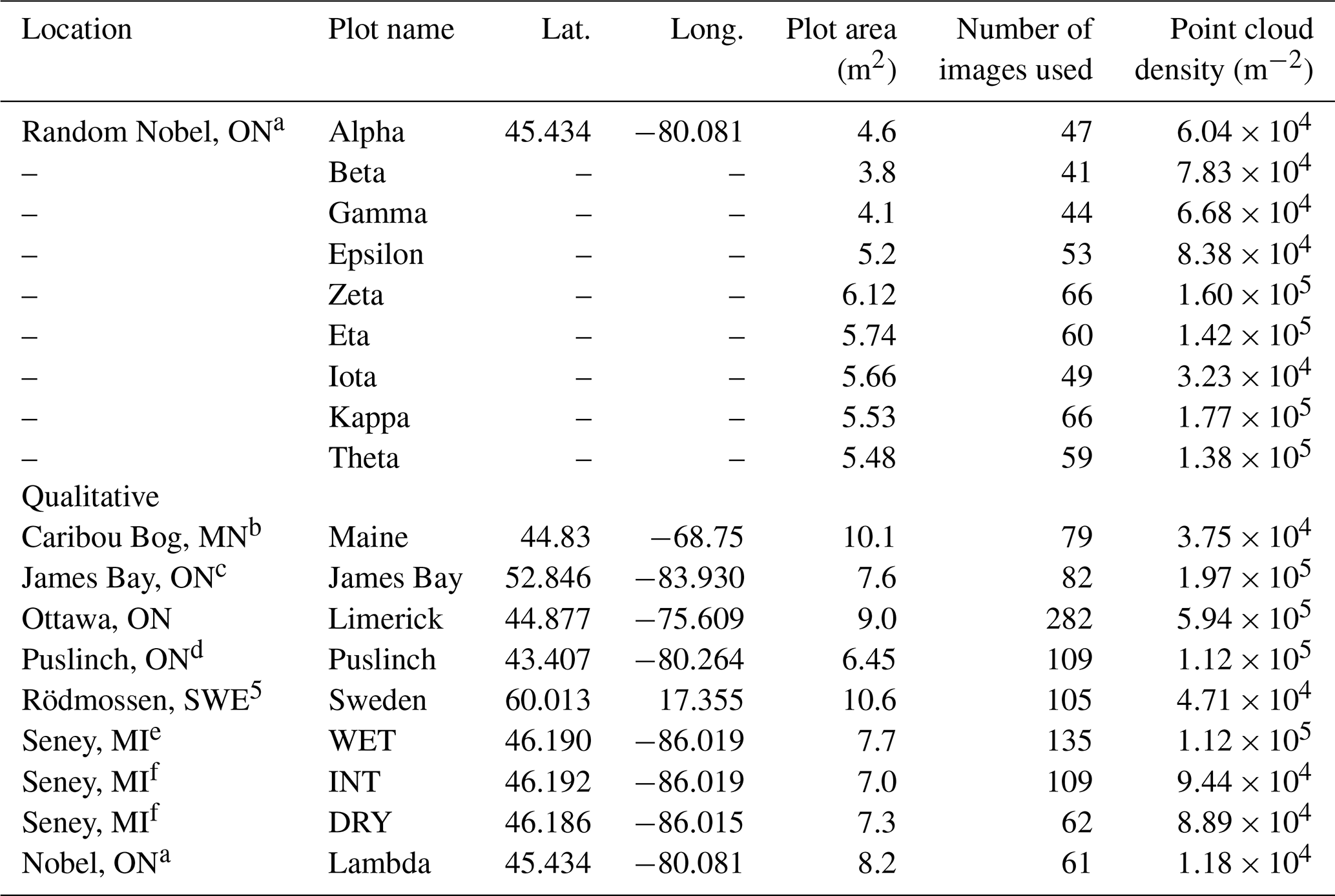
For detailed site information, see the following studies. a Moore et al. (2019a). b Kettridge et al. (2008). c Ulanowski and Branfireuen (2013). d Campbell et al. (1997). e Granath et al. (2009). f Moore et al. (2015).
2.2 Site preparation and image acquisition protocol
All vascular vegetation was removed from the plot area using scissors and hand pruners in order to provide an unobstructed view of the surface microtopographic variation (moss surface) for imaging. Matte-colored disks (n=20) of 0.04 m diameter were placed randomly on the clipped surface to provide reference points for better correlation between images. To provide absolute scale and orientation, two boxes of known dimensions (0.1 m × 0.1 m × 0.1 m) were placed in each plot and leveled prior to image acquisition. Images of each target area were taken via at least two circuits around the plot, with images taken from two separate vertical viewing angles (see https://www.cs.cmu.edu/~reconstruction/basic_workflow.html, last access: 3 September 2019, for third-party description of general workflow). Distance to target area was set so that a large portion of the clipped area was visible in each image. To produce different horizontal viewing angles, images were taken every one or two paces around the perimeter of the plot. This procedure yielded 41 to 282 overlapping images from multiple viewpoints of the plot areas, which ranged in size from 3.2 to 10.1 m2 (Table 1). Images were taken during either clear-sky or overcast conditions near midday during the summer to avoid changing lighting conditions and to limit self-shadowing of the surface. Images were captured with digital cameras using automatic exposure settings. Prior to analysis, all images were downscaled where necessary to a common resolution of 2048×1536 pixels using a Lanczos3 filter.
2.3 Digital elevation models of microtopography
A point cloud of the moss surface was generated using an SfM approach (Brown and Lowe, 2005; Mercer and Westbrook, 2016) using the program Visual SfM (Wu, 2011). Visual SfM identifies image features for cross-comparison using a scale-invariant feature transform (Lowe, 1999) and then matches features between images in a pairwise manner. Effectively, this creates multiple stereo-pairs from which camera position and scene geometry can be estimated through triangulation. This procedure yielded average point cloud densities ranging from 3 to 59 pixels cm−2 for the imaged plots (Table 1).
Prior to generating the DEMs, point clouds were cropped to the region of interest (i.e. area of clipped vegetation), then scaled, leveled, and oriented using the rendered reference objects. DEMs were produced using the MATLAB function TriScatteredInterp (MATLAB R2010a, MathWorks), which performs Delaunay triangulation of the point clouds. DEMs were generated on a 0.01 m × 0.01 m grid using natural neighbour (Voronoi) interpolation. The DEMs were smoothed using a mean filter window with a size of 0.03 m × 0.03 m. Finally, a mask was applied to the DEMs to remove reference objects. The accuracy of the method was assessed (see Sect. S1 in the Supplement and corresponding Figs. S2 and S3 in the Supplement), yielding root mean square error values less than 0.01 m in the x, y, and z directions under laboratory conditions. Median absolute deviation of elevation between the DEM and lab and field validation plots was 0.004 and 0.018 m, respectively.
2.4 Capturing site-level microtopographic variation
Plots from the Red Earth Creek peatland were ∼3.5 m2, and differences between plot elevation for the 50 plots were surveyed using a Smart Leveler digital water level (accuracy of ± 2.5 mm), with offsets applied to DEMs. A Monte Carlo resampling approach was used to evaluate how total variance in microtopographic elevation increased with increasing sample size. For each sample size (i.e. 1–50), 200 random resamplings were performed. To estimate the change in variance with increasing sample size, a rectangular hyperbola was fit to the mean variance (y) versus sample size (x):
where b is the estimated maximum total variance, and a and c are initial slope and concavity parameters.
To evaluate the dominant scale of microtopographic variation which contributes to total variance, a fast Fourier transform (fft function in MATLAB) was used to estimate the power spectral density (PSD) of microtopographic variation along an artificially constructed 300 m long transect (combination of multiple transects; see Fig. S1, middle panel). Manual measurements of moss surface elevation were taken every 0.05 m along multiple connected transects at the Red Earth Creek, AB, and Nobel, ON, site using the Smart Leveler.
2.5 Plot-level microtopographic variation
Plot-level microtopographic variation was analyzed using randomly and qualitatively chosen plot locations listed in Table 1. Based on the hummock–hollow conceptual model, our a priori assumption was that a hummock–hollow pair would have a bimodal distribution of surface elevation. Our null hypothesis was that microtopography would follow a bimodal distribution, so we evaluated DEM height distributions using one- to three-member Gaussian mixture models (GMMs) to evaluate whether two-member GMMs would best explain height distributions. GMMs were fit to DEM height distributions using the MATLAB function gmmdistribution.fit, which uses an iterative expectation maximization algorithm to determine GMM parameters representing maximum likelihood estimates. The GMM fit function was seeded with initial parameter estimates using k-means cluster analysis. The best model was selected based on the minimum Akaike information criterion (AIC).
Surface slope and aspect were evaluated using the computed surface normals for each point and eight connected neighbours of the DEM. The fractal dimension of plots was evaluated using radially averaged PSD derived from an fft of elevation data. The Hurst (H) exponent (values of 0–1) presented herein is related to fractal dimension as 3−H, where the slope of the PSD curve in log space is .
2.6 Modeled moss surface insolation and productivity at the plot level
Potential moss surface insolation was modeled using the formulation presented in Kumar et al. (1997) to account for Earth–Sun geometry, surface slope and aspect, and diffuse radiation under clear-sky conditions. Total potential insolation was evaluated on an annual basis and normalized relative to total insolation on a flat surface for each plot location.
For moss net photosynthesis (NP) and capitula water content (WC), each plot was classified into three units based on relative elevation which notionally correspond to hollow/lawn, low hummock, and high hummock. The k-means clustering was used to perform unsupervised classification of microtopographic elevation (Fig. S4). A separate parameterization for moss NP and WC was used for each elevation cluster. Parameterizations for hollow/lawn, low hummock, and high hummock were obtained from Sphagnum species of the section Cuspidata, Sphagnum, and Acutifolia, respectively (Fig. S5). Empirical relations between WC and water table depth (WTD) were derived from Strack and Price (2009) and Rydin (1985), and were modeled as follows:
where WC is the ratio of the mass of water to the sample dry weight (g g−1), and p1−3 are fitted parameters. WC was restricted to a range of 1–25 g g−1. A rational function was used to model the relation between moss capitula NP and WC according to the results in Schipperges and Rydin (1998), where
where NPpot represents percentage of maximum NP, and p4−8 are fitted parameters. Estimates of 2.7, 5.6, and 6.5 g m−2 d−1 for NPmax were used to represent Sphagnum species of section Cuspidata, Sphagnum, and Acutifolia, respectively (Nungesser, 2003).
3.1 Site-level microtopographic variation
In characterizing microtopographic variability across the Red Earth Creek site (Fig. S1 – middle panel), our data show that variability in surface elevation increases asymptotically with sample size (i.e. area sampled) and is well predicted by a rectangular hyperbola (r2=0.98; p≪0.01) (Fig. 1). Based on the asymptote of the fitted rectangular hyperbola (0.147 m), Fig. 1 shows that on average an area of 32 m2 (i.e. nine random plots of ∼3.5 m2 size) contains roughly 95 % of the predicted site-scale microtopographic variability. Even though increasing the number of plots by a factor of 5 (i.e. ∼50 plots) has little effect on the average variance in surface elevation, the range associated with resampling is reduced by about half (Fig. 1 – shaded area).
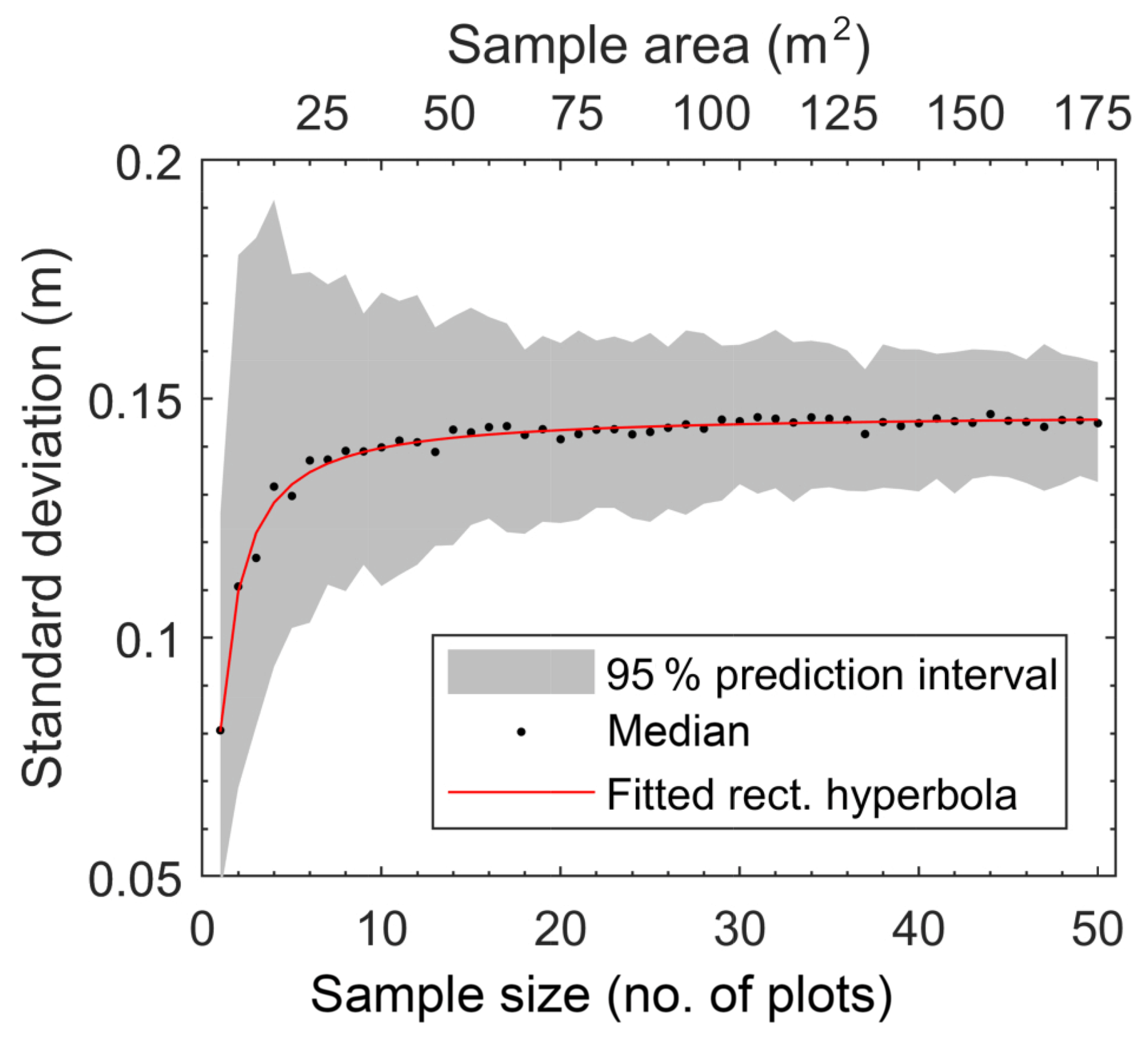
Figure 1Site-level relation between standard deviation of microtopographic variation based on total sample area for the Red Earth Creek site based on 50 ∼3.5 m2 plots. The grey shaded area represents the 2.5th and 97.5th percentiles of standard deviation from the Monte Carlo resampling procedure.
While the Red Earth Creek multi-plot DEM data provide the ability to assess the area required to capture site-scale microtopographic variability for a small unpatterned Alberta peatland, they do not directly provide information on what spatial scales contribute most to overall variability. The PSD of manual elevation transects from both the Red Earth Creek and Nobel sites suggests that most of the microtopographic variation for these two surveyed sites occurs at spatial scales between 1 and 10 m (Fig. 2 – cumulative curves). Both sites have qualitatively similar PSD curves in log space with a roll-off at spatial scales between 2.4 and 2.9 m (break point of piecewise regression). Moreover, the PSD of microtopographic variation appears to be well described by a power law (i.e. relatively smooth slope in log space despite noise) at small spatial scales resulting in a Hurst exponent (see methods section for relation to fractal dimension) between 0.14 and 0.26. For both transects, 95 % of total variance is captured at a length scale greater than ∼0.6 m.
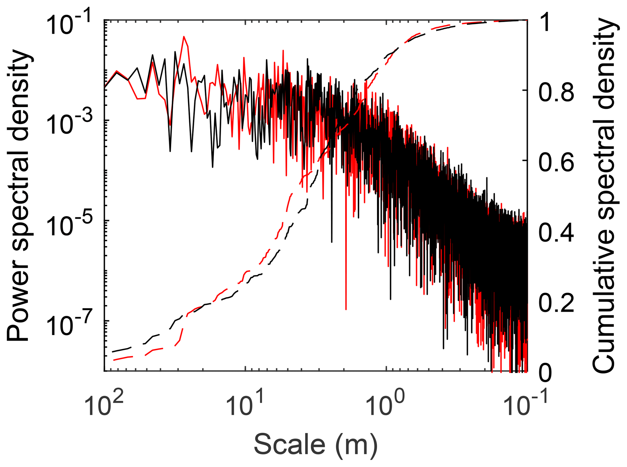
Figure 2Site-level absolute (solid lines) and cumulative (dashed lines) power spectral density of height along a 300 m transect for the Red Earth Creek, AB (red), and Nobel, ON (black), sites.
3.2 Plot-level hypsometry and fractal dimension
There is a characteristic difference in the elevation distribution of whole plots compared to that of the corresponding hummock–hollow subplots for both qualitatively (Fig. 3) and randomly (Fig. 4) chosen plot locations. The elevation distributions for hummock–hollow subplots tend to have a clear separation of modes (Figs. 3b and 4b). The degree of separation in modes has a moderately weak correlation (r2=0.31) but significant linear relation (F16=7.1, p=0.017) with the interquartile range in elevation of the whole plot. On average, the elevation range absent from the hummock–hollow subplots represents roughly 31 % of the microtopographic range of the whole plot. When all hummock–hollow subplots are aggregated across randomly selected plots (i.e. Nobel, ON, site), the whole elevation distribution is captured (Fig. S6). However, there remains a bias towards higher elevations being sampled in the aggregated subplot elevation distribution compared to the aggregated whole plot elevation distribution.
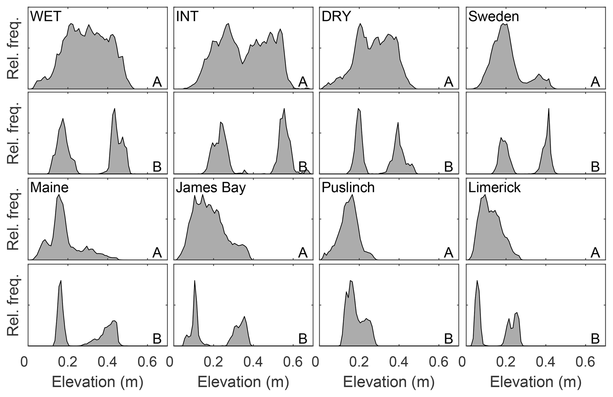
Figure 3Plot-level relative frequency distribution of height in plots where a perceived representative hummock and adjacent hollow was subjectively chosen for a given site (Table 1 – qualitative plot locations). Relative height distributions are shown for all of panel (a) and for a hummock and hollow panel (b), whose area corresponds to the size of a large flux measurement chamber. Elevations are referenced to the lowest point of the reconstructed surface and set to zero.
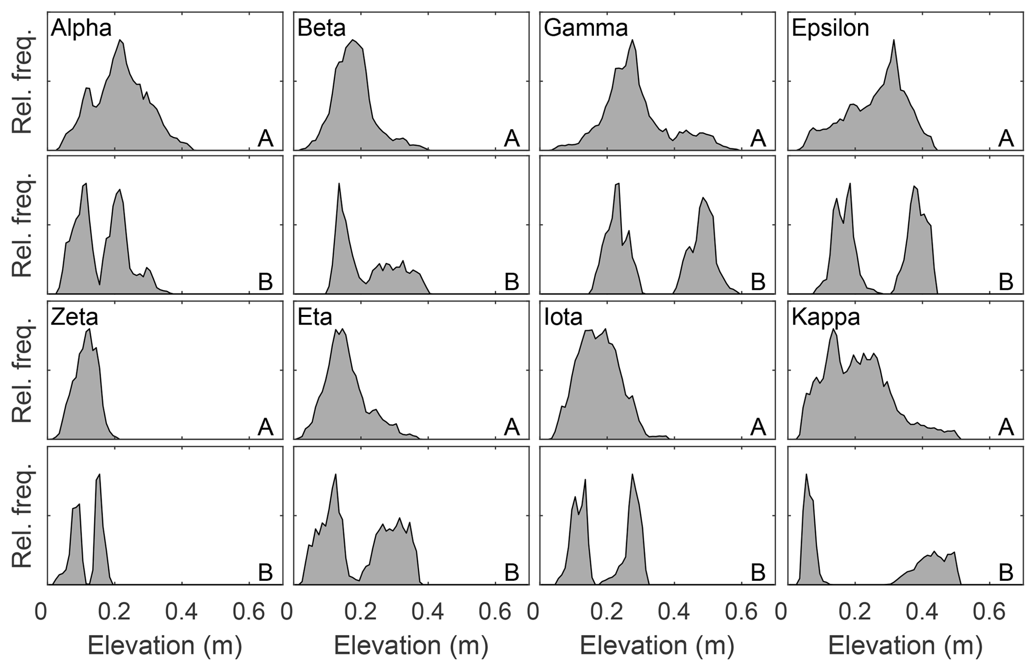
Figure 4Plot-level relative frequency distribution of height in plots with randomly chosen locations within a site containing a perceived hummock and adjacent hollow (Table 1 – random plot locations). Relative height distributions are shown for all of panel (a) and for a hummock and hollow panel (b), whose area corresponds to the size of a large flux measurement chamber. Elevations are referenced to the lowest point of the reconstructed surface and set to zero.
In testing the null hypothesis of bimodally distributed relative surface elevation at the plot scale, we examined the goodness of fit of one-, two-, and three-member GMMs (see Fig. S7 for example GMM fits). An assessment of all 18 plots suggests that two- or three-member GMMs tend to provide a better fit to reconstructed elevation distributions compared to a one-member (i.e. normal) distribution. Based on AIC values, the one-member GMM was best for only three plots, while two- and three-member GMMs were best for six and nine plots, respectively (Table 2). In contrast, when GMMs were fit to hummock–hollow subplot data, the two-member GMM tended to outperform one- and three-member GMMs.
Table 2Estimated parameters for one-, two-, or three-member GMM fit to elevation distribution of plot-level digital elevation models. Results are presented for the GMM which minimizes AIC. Plots are separated into those chosen at random versus qualitatively at their respective site.
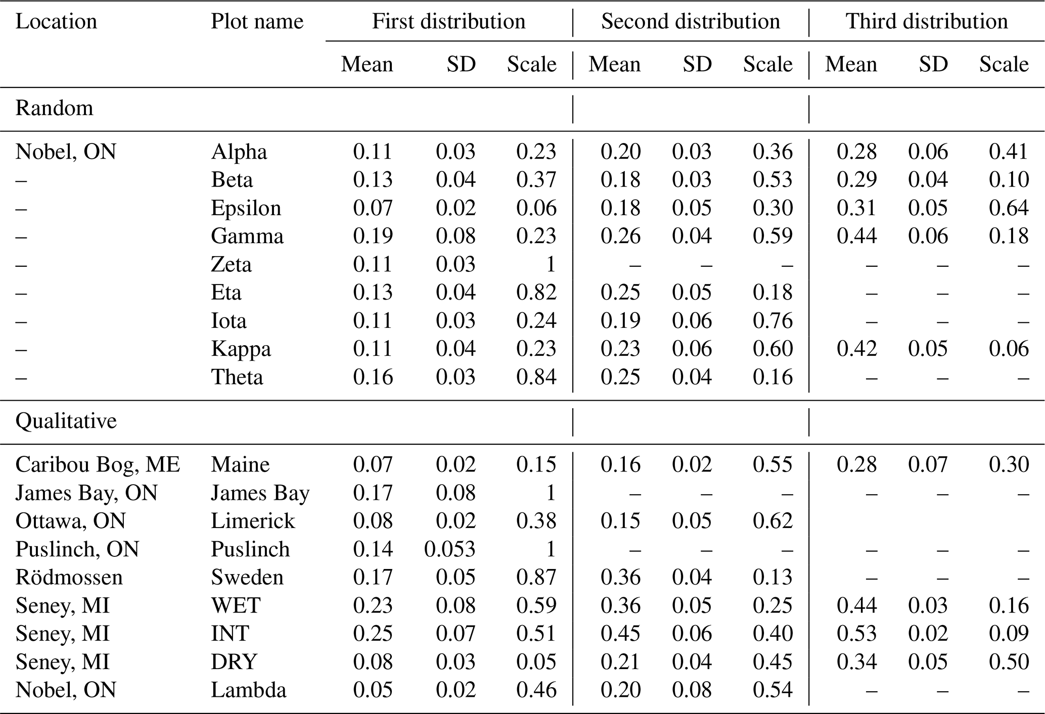
The mean (μ) and standard deviation of elevation for hummock and hollow subplots were grouped and compared according to plot selection method (i.e. random within-site versus qualitative between-site selection). Since the μ parameter corresponds to relative elevation, we took the difference between the two members (i.e. μhum−μhol) for comparison purposes. Overall, the qualitatively chosen plots appear to have similar relative hummock heights (μhum−μhol) (0.21±0.08 m) compared to the randomly chosen plots (0.19±0.09 m) (; p=0.66). Variation in elevation tended to be higher in hummock subplots (0.031±0.012 m) compared to hollow subplots (0.021±0.008 m) (microform; , p=0.005), where the difference between hummock and hollow subplots was similar when comparing qualitatively and randomly chosen sites (microform and plot type interaction; ; p=0.82).
Depending on the underlying structure of spatial variability, surface roughness can be highly dependent on the scale of analysis. A two-dimensional power spectral density of elevation provides a means to formally describe the change in roughness with scale (Fig. 5). The power spectral density of elevation was found to be a linear function of length scale across the 0.05–1 m range in log–log space () and is the basis for the Hurst exponent (H) (see methods section for relation to fractal dimension). While the distribution of H for qualitatively chosen plots (0.70±0.18) was higher compared to randomly chosen plots (0.58±0.10) (i.e. comparatively less “complexity” at finer spatial scales), the difference was not significant (; p=0.10). Similar to the transect-based analysis (see site-level microtopographic variation section), 95 % of total variance is captured at a length scale greater than 0.37–0.90 m.
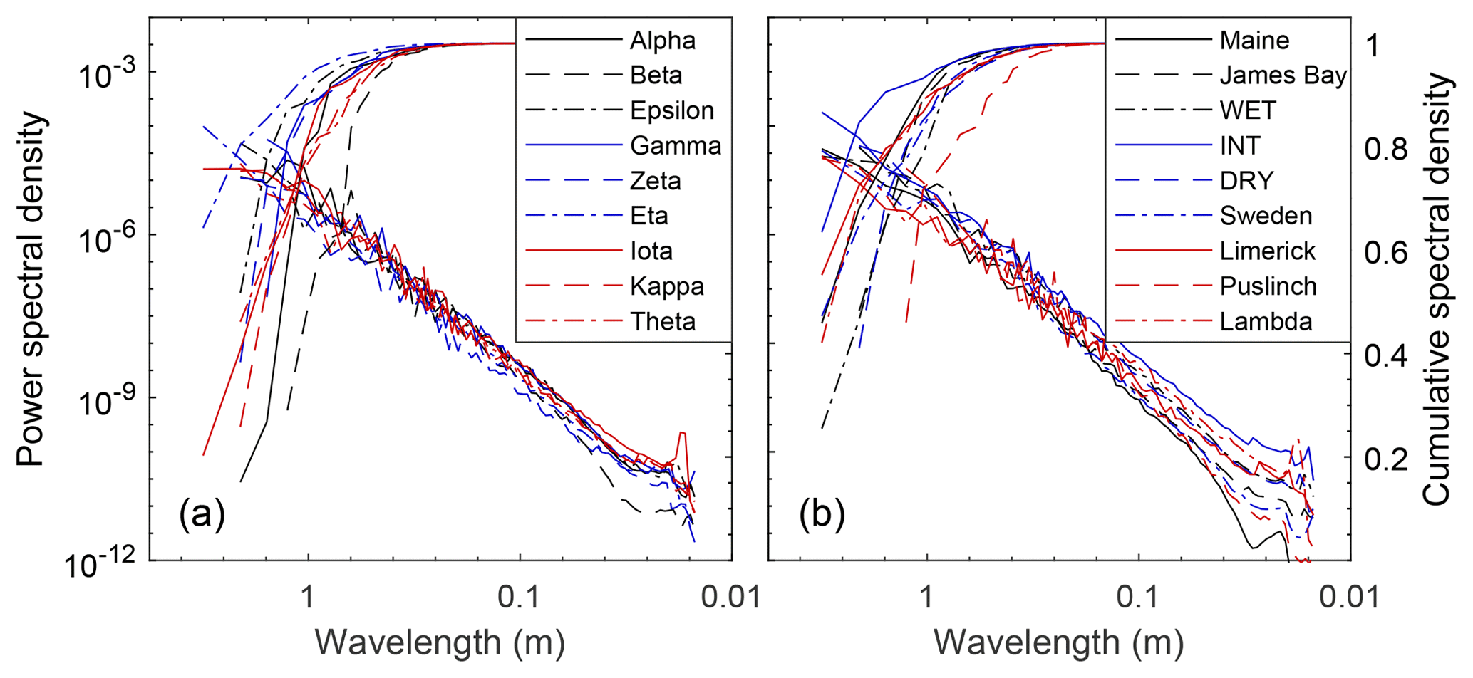
Figure 5Plot-level radially averaged power spectral density for randomly (a) and qualitatively (b) chosen plots (Table 1) representing the change in elevation variability with length scale. The slope between the power spectral density and wavelength in log–log space corresponds to the Hurst exponent (H), where slope = , and is related to the fractal dimension as 3−H.
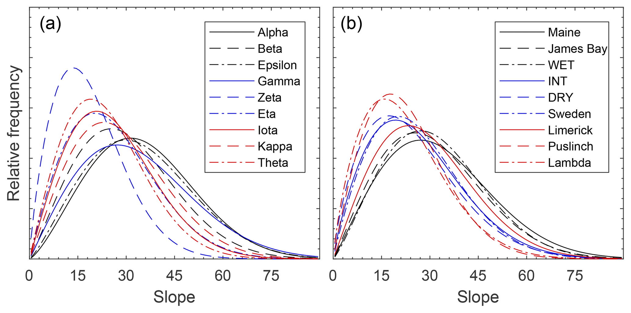
Figure 6Plot-level Weibull probability density function of slope derived from the surface normal of a planar fit to elevation in a moving 0.03 m × 0.03 m window for all DEMs. Panels (a) and (b) separate the randomly and qualitatively chosen plots, respectively.
3.3 Plot-level slope, aspect, and solar insolation
A Weibull distribution provided a good fit to the slopes for the reconstructed DEMs (Fig. S8), where the average, maximum, and minimum RMSEs were 0.10 %, 0.14 %, and 0.06 %, respectively, based on a relative frequency distribution with 1∘ bin sizes. When grouped according to qualitatively versus randomly chosen plots (Table 1), the modal slope for whole plots was 18.6±4.5 and 20.0±4.8∘, respectively. Similarly, the distribution of standard deviation in slope for qualitatively and randomly chosen plots was 13.1±1.5 and 12.9±2.0∘, respectively. Comparing the parameter distributions from the Weibull fit for qualitatively and randomly chosen plots (Fig. 6), it was found that there was no significant difference in the mean scale (analogous to mode) and shape (analogous to standard deviation) parameters (scale: p=0.72, ; shape: p=0.24, ).
While modal slope tended to only be slightly higher in the hummock subplots (20.3±6.9∘) versus hollow subplots (16.0±5.1∘), there was greater distinction in the prevalence of steep slopes (i.e. >45∘) in hummock subplots (8.7±8.6 %) versus hollow subplots (3.4±5.4 %) (Fig. S9). Comparing slope in the hummock–hollow subplots to the three-member GMM clusters (high, intermediate, and low elevations; for example, see Fig. S4), we see that the subplots tend to be somewhat flatter compared to the rest of the plot, particularly for hollow subplots (Fig. S9).
Figure 7 shows how slope and aspect of the Seney WET plot affect potential solar insolation at the moss surface under ideal conditions (i.e. clear-sky, sparse vegetation), where broadly similar results are obtained for all plots (Fig. S10). Potential solar insolation is significantly affected by aspect (, p≪0.01) (e.g. Fig. 7a) and its interaction with slope (, p≪0.01) (e.g. Fig. 7b) across all plots, where, on average, south-facing slopes receive double the potential solar insolation compared to north-facing slopes. Based on measured slope and aspect at randomly and qualitatively chosen plots, median potential solar insolation for a south-facing slope is 14 %–25 % greater compared to a flat surface. Similarly, for a north-facing slope, median potential solar insolation is 21 %–45 % lower (Fig. S10).
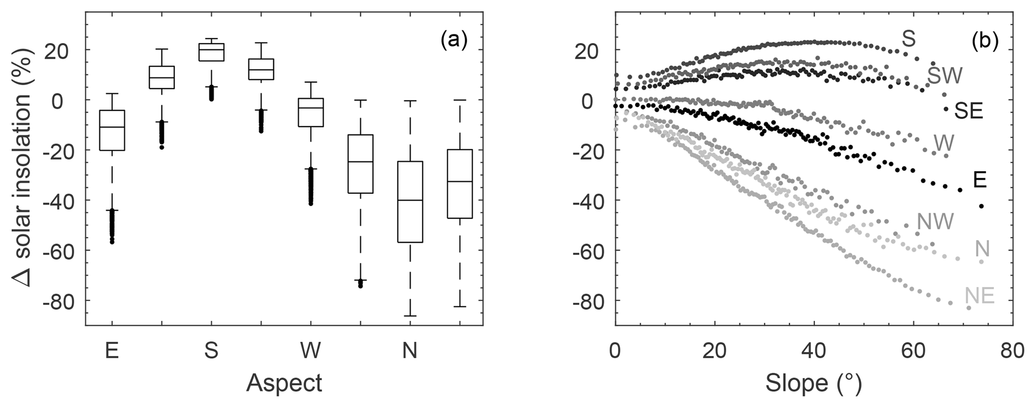
Figure 7Variation in potential solar insolation relative to a flat surface based on aspect (a) and slope (b). Box plots show median and interquartile range, with outliers shown as dots. Insolation as a function of slope has been bin averaged per cardinal direction, where each point represents 100 data points. Slope and aspect data are for the Seney WET plot.
3.4 Plot-level empirical model of moss productivity using high-resolution DEMs
Assuming a flat water table at the plot level, Fig. 8 shows how modeled NPpot varies with WTD relative to the average hollow surface. Hollows tend to have a comparatively narrow range of WTD (i.e. 0–0.15 m) over which the moss is expected to be highly productive compared to hummocks. Despite using species-dependent NPpot–WC relations, the large differences in water table range over which hummock and hollow NPpot is high is largely driven by the WC–WTD relations (Fig. S5). Where moss species have large differences in NPmax and different characteristic water retention, NPpot rarely overlaps between microtopographic classes (Fig. 8). If we ignore the effect of species-dependent characteristics (i.e. NPmax, NPpot–WC, and WC–WTD) and use a single parameterization (herein low hummock), differences between microtopographic classes tend to be smaller for shallow water table conditions (Fig. S11), yet there remains a characteristic difference in mean NPpot between microtopographic classes.
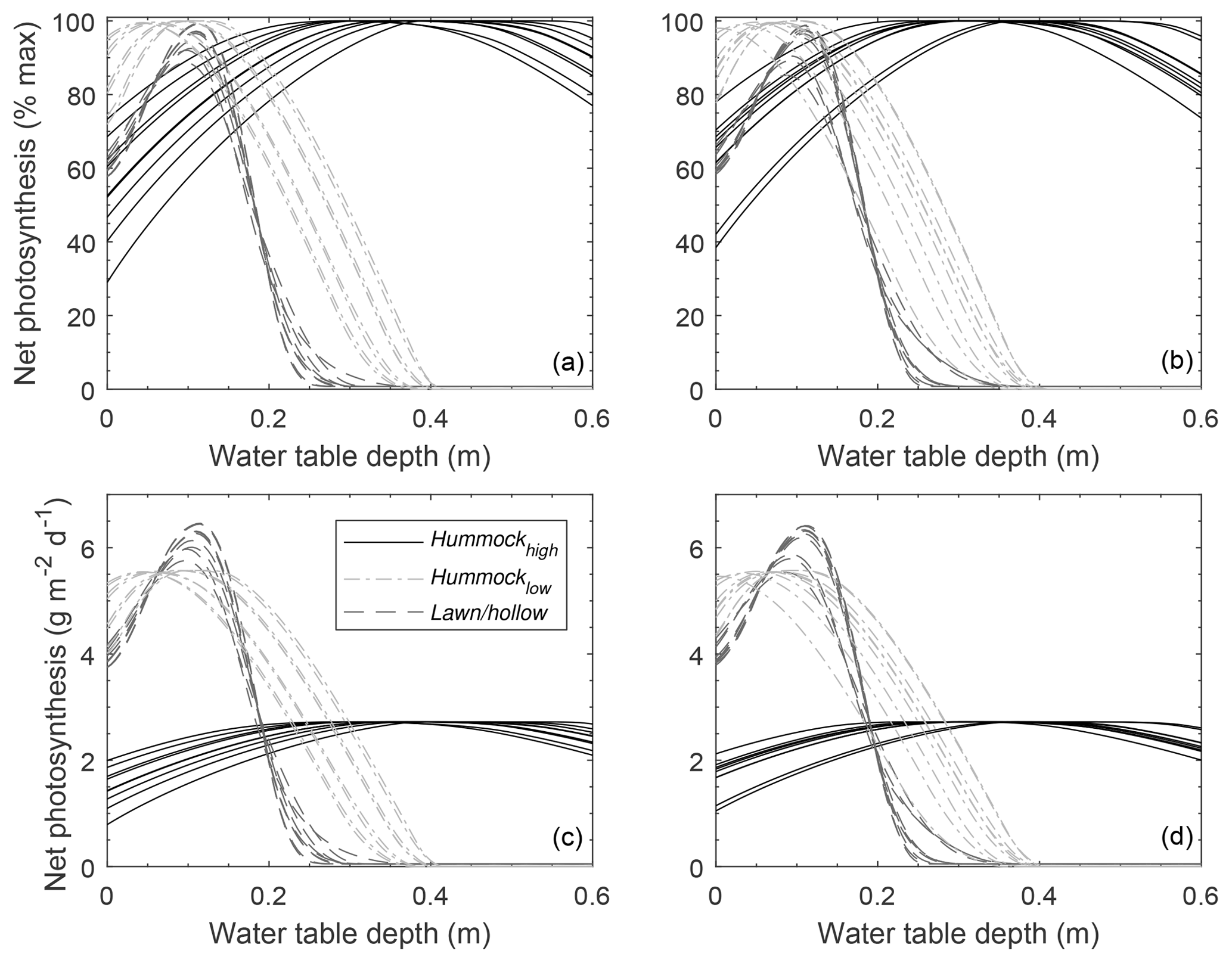
Figure 8Plots-scale mean potential net photosynthesis (NP) for three microtopographic classes (i.e. high-hummock, low-hummock, and lawn/hollow; see Fig. S4) derived from spatially explicit elevation data for random (a, c) and qualitatively chosen (b, d) plots. NP-WC and WC-WTD relations are based on separate parameterization for each microtopography class (see Fig. S5).
From a scaling perspective, modeled NPpot (Figs. 8 and S11) was used to compare spatially explicit estimates with averages based on the notional chamber subplot (i.e. pre-determined 0.37 m2 area in perceived hummock and hollow; see methods and Fig. S1, lower panel). In general, spatially explicit NPpot estimates tended to be higher/lower than the scaled hummock–hollow subplot estimates depending on whether the water table was relatively shallow/deep (Fig. 9a). The maximum positive bias between the spatially explicit and scaled hummock–hollow subplot NPpot values ranged from 0.52 to 1.37 g m−2 d−1 under shallow water table conditions, while the negative bias ranged from −0.22 to −1.98 g m−2 d−1 under deeper water table conditions. Using a single parameterization for NPpot tends to result more consistently in positive bias between the spatially explicit and scaled hummock–hollow subplot models (Fig. 9b), where maximum bias is up to 1.98 g m−2 d−1. Averaged across all 18 plots, the location of the subjective hummock subplot broadly overlapped with the k-means high-hummock classification (94 %), with only small portions overlapping with the low-hummock classification (6 %). Similarly, the location of the subjective hollow subplot broadly overlapped with the k-means hollow/lawn classification (79 %), with only small portions overlapping with the low-hummock classification (20 %). In this study, our results indicate that the subjective choice of hummock and hollow subplot location (e.g. for chamber flux measurement) systematically undersamples intermediate topographic positions. For the NPpot model using separate parameterization for the microtopography classes, the low-hummock class tends to remain distinct from both the hollow/lawn and high-hummock class except under very dry conditions (see Fig. S12 for an example). For the uniform parameterization, the low-hummock classification is distinct from the other two classes only under wet conditions. In contrast, the low-hummock classification behaves like the hollow/lawn under moderately dry conditions and behaves like a high-hummock classification under very dry conditions.

Figure 9Difference in plot-scale potential net photosynthesis (NPpot) between models using the measured distribution of elevation over the entire SfM-derived DEM and the measured distribution within hummock–hollow subplots. NPpot is modeled using separate parameterization (see Fig. S5) for each microtopography class (a), as well as a uniform (low-hummock) parameterization across microtopography classes (b).
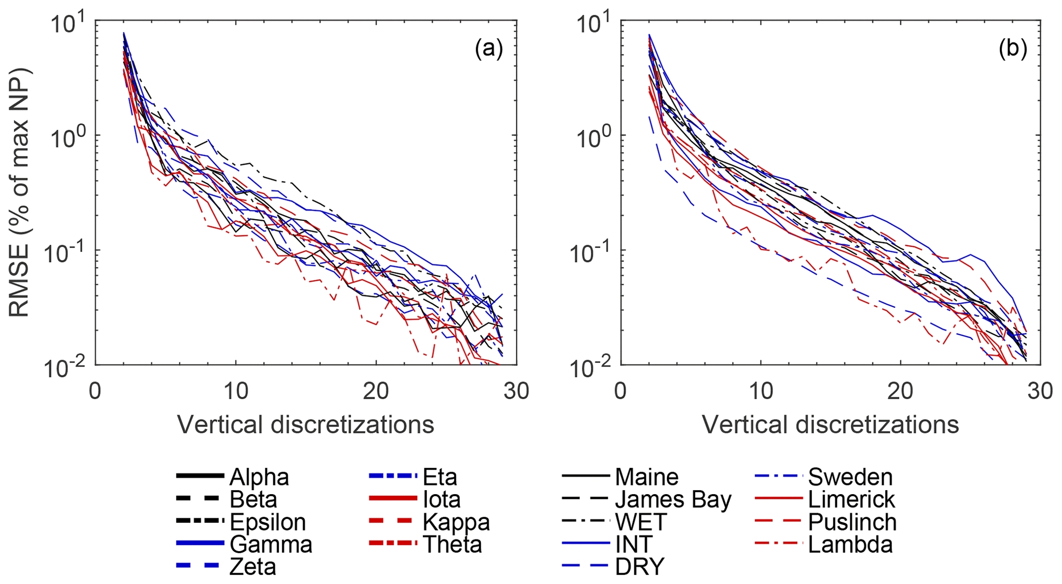
Figure 10Difference in plot-scale potential net photosynthesis (NPpot – as a percentage of max) based on a coarse to fine discretization of elevation values (nz=2 to 30) (see Fig. S13 for example). NPpot is modeled using separate parameterizations (see Fig. S5) for each microtopography class (a), as well as a uniform (low-hummock) parameterization across microtopography classes (b). RMSE was calculated using NPpot from the original plot-level DEMs as the reference values. Discretized elevation values for each plot are based on elevation percentiles (pz,i), where , for i=1 to nz.
Evaluated over a large range of WTD (i.e. 0–0.6 m below average hollow surface), the root mean square difference (RMSD) between NPpot (as % of maximum) calculated using the SfM-derived DEMs and binary classification using the average hummock and hollow subplot elevation was 20±6 %. However, bias between the DEM-based NPpot and subjective hummock–hollow elevations is greatly reduced if an unbiased binary classification is used. The RMSD when hummock and hollow elevations are set to the 66th and 33rd percentiles of measured elevation distribution is reduced 5±2 % (Fig. 10). Moreover, bias is largely eliminated with the use of only several elevation classes where, for example, an RMSD of 1 % or less is achieved using two to seven elevation classes.
4.1 Assessing microform representativeness
In studies which use the hummock–hollow microtopography classification as part of their sampling design, there are many cases in which the plot choice is said to be representative (e.g. Kettridge and Baird, 2008; Laing et al., 2008; Nijp et al., 2014) but often lacks detail on how representativeness was assessed. For example, when characterizing the surface within an eddy covariance flux measurement footprint, it is common to only sample one or few hummock–hollow pair(s) (e.g. Lafleur et al., 2003; Humphreys et al., 2006; Peichl et al., 2014; Moore et al., 2015). Similarly, for direct measurements of surface fluxes where microtopography is considered explicitly, chamber-based measurements typically use between four and eight replicates (e.g. Frenzel and Karofeld, 2000; Turetsky et al., 2002; Forbrich et al., 2011; Petrone et al., 2011) per microtopographic unit. For peatland studies which use random plots, as many as 30 plots per site have been reported (i.e. Wieder et al., 2009), yet earlier studies have reported using as few as one to four plots to characterize a site (e.g. Crill et al., 1988; Shannon and White, 1994; Regina et al., 1996). Using the Red Earth Creek results as a reference, for studies which have four to eight replicates, two to three microtopographic units (e.g. hummock, lawn, hollow), and the more common chamber size of roughly 0.6 m × 0.6 m, we would infer from our results that the typical total sample area for chamber flux measurements in a peatland ecosystem would capture on the order of 70 %–86 % of site-scale microtopographic variability in their plots. It should be noted, however, that the simple assessment above assumes that chamber placement is random. In cases with lower replication of two microtopographic units, our results suggest that the uncertainty associated with repeated sampling is relatively high (Fig. 1 – shaded area) and that the choice of two microtopographic units could lead to an undersampling of intermediate topographic positions (e.g. Figs. 3b and 4b). When the ecosystem processes of interest are not measured across the range of variability observed at the site scale, particularly for non-linear processes, then scaling from process-based, or simply plot-scale, measurements is at risk of being biased. Our simple empirical model of moss NPpot demonstrates that flux bias can be large relative to NPmax and is strongly dependent on water table depth (Fig. 9). While water table is a first-order control on peat water content (Hayward and Clymo, 1982), moss capitula water content, however, has been shown to be less sensitive to water table (Strack and Price, 2009). Moreover, the sensitivity of Sphagnum CO2 assimilation to water level has been shown to be strongly dependent on precipitation (Robroek et al., 2009). Using the simple empirical model and measured WTD at the Seney site (see Moore et al., 2015), the magnitude of modeled NPpot (seasonal average of 1.2–3.8 g m−2 d−1) is less than seasonal average chamber-measured gross primary productivity (GPP) values (see Ballantyne et al., 2014), though the later includes vascular vegetation. Nevertheless, the empirical NP-modeled values are broadly consistent with field measured Sphagnum production (e.g. Moore, 1989; Waddington et al., 2003). Although NPpot estimates are strongly influenced by the parameterization used (e.g. Figs. 8 and S11), there remains a large bias between the spatially explicit and scaled hummock–hollow subplot NPpot models.
To upscale models or plot-scale measurements, it is important to determine the microtopographic structure and variability of a peatland. There were often non-bimodal distributions of microtopography in our study sites (Figs. 3a and 4a and Table 2) where the more continuous distribution of elevation at the plot scale suggests that when experimental designs use hummock–hollow pairs as the primary experimental unit (Figs. 3b and 4b), they have a tendency to capture the ends of the distribution, omitting on average 25 % of the elevation distribution at the plot scale (see also Fig. S6). In this study, we clipped vegetation in 50 small random plots to produce very-high-resolution DEMs for assessing microtope-scale (i.e. S3 hummock–hollow complex; see Belyea and Baird, 2006) variability, yet surface vegetation removal will generally be undesirable. Ground- or drone-based SfM approaches have been used to produce a digital surface model (DSM – vegetation present) for alpine (Mercer and Westbrook, 2016) and blanket (Harris and Baird, 2018) peatlands with reasonable accuracy (e.g. mean absolute error of ∼0.08 m, and normalized median absolute deviation of ∼0.11 m for the alpine and blanket peatlands, respectively). In situations where surface vegetation removal is not possible or desirable and/or where drone-based imagery is hampered (e.g. treed peatlands), a survey of height distribution along one or several transects would provide an alternative to assessing microtope- to mesotope-scale (S3–S4; Belyea and Baird, 2006) microtopographic variability. The power spectral density of transect data would suggest that, for absolute height, a sampling interval of less than 1 m (e.g. 0.5 m) would capture the scales of variability which contribute most to total height variance (Figs. 2 and 5), since this corresponds to ∼95 % of measured microtopographic variation, and provide sufficient fine-scale data to estimate the fractal dimension of microtopography. Information on height distributions could provide the basis for plot selection, where plots could be chosen to deliberately span the range of variability or to avoid oversampling extremes. Information on the height distribution would furthermore provide the ability to scale up findings from the plot level given their relative position in the wider distribution of microtopographic variability (see Griffis et al., 2000).
Despite the variety of site characteristics observed, our plots were limited to bogs and poor fens, and did not include sites with ridge and pool patterning. Nevertheless, our results would suggest that generalizations based on a hummock–hollow classification, either to the site scale or to hummock–hollow pairs across sites, should be viewed with a degree of skepticism when sample size is low or when a general microtopographic survey is absent/unreported. Thus, for wider intercomparability of peatland studies, SfM or transect-based approaches of measuring and reporting on one or several morphometric properties of microtopography could provide a more comprehensive dataset to aid in future meta-analysis/synthesis.
4.2 Implications for appropriate complexity ecosystem modeling in peatlands
The complex shape/structure of peatland microtopography has generally been ignored from a modeling standpoint, but several studies have shown, for example, that slope and aspect may affect peat temperature (Kettridge and Baird, 2010). Under clear-sky conditions, modeled annual total solar insolation differs from a flat surface by roughly ±20 % in our measured plots, where our study sites span 43 to 60∘ N latitude (Fig. S10). For north- and south-facing slopes, this effect is amplified (Fig. 7) particularly for high- and low-hummock microtopographic classes (e.g. Fig. S4), which tend to have greater average slope compared to the hollow/lawn classification (Fig. S9). While our study sites are limited to the non-permafrost boreal region, the applicability of slope and aspect considerations to modeling tundra tussocks in arctic and permafrost regions is also relevant (e.g. De Baets et al., 2016). Based on the results of empirical studies, the shape of microtopographic features ought to play a role in ecosystem fluxes due to the effect of shortwave radiation on surface evaporation (Kettridge and Baird, 2010), photosynthetically active radiation on moss production (Harley et al., 1989; Loisel et al., 2012), and soil temperature on methane production and respiration (e.g. Lafleur et al., 2005; Waddington et al., 2009). It is important to note, however, that under cloudy conditions the increasing proportion of total insolation from diffuse radiation decreases the disparity in insolation associated with slope and aspect. Furthermore, in peatlands where substantial tree, shrub, or graminoid cover exists, the importance of slope and aspect on soil heating or ecosystem fluxes is likely to be low since insolation decreases exponentially with increasing vascular leaf area.
In addition to microtopographic shape/structure, the size of microtopographic features and their small-scale variability can similarly affect ecosystem fluxes, where height above water table imposes a first-order control on water availability. Methane fluxes from peatlands, for example, have been shown to vary logarithmically over 0.1 m scales (Turetsky et al., 2014). Water availability at the moss surface has been shown to be both species-dependent and strongly affected by water table (Hayward and Clymo, 1982; Rydin, 1985), where moss species and water availability have been linked to many ecohydrological processes such as surface evaporation (Kettridge and Waddington, 2014), productivity (Williams and Flanagan, 1998; Strack and Price, 2009), and hydrophobicity (Moore et al., 2017). We show that when microtopographic variability is explicitly modeled, complex patterns of potential moss productivity emerge (Fig. S12) which are not necessarily captured by a hummock–hollow model (Fig. 9), and that the presence of bias is independent of whether moss species niche partitioning is considered.
The SfM method is a potentially useful tool for examining how morphometric properties of the surface which affect ecohydrological processes vary within a site. Moreover, information on microtopographic variability from SfM-derived DEMs can be used to further examine the potential role of fine-scale microtopographic variability on biogeochemical processes within a modeling domain. The GMM is a simple way to include a more realistic description of height distributions within distributed peatland models (e.g. Dimitrov et al., 2010) or extend from the meso- to micro-scale (Sonnentag et al., 2008). Computationally, GMMs are a relatively efficient way of representing microtopographic variability, needing only two parameters per member of the GMM distribution. Conceptually, the GMM distribution can be applied directly in distributed peatland models to populate relative heights of individual cells. In the case of one-dimensional models, a GMM distribution can be used as a transfer function for any water-table-dependent processes, particularly in cases where the relation is non-linear. Alternatively, a small number of parameters from the PSD of microtopographic elevation (e.g. variance, Hurst exponent, and spatial scale of break point), be it from a transect (Fig. 2) or DEM (Fig. 5), can be used to generate “synthetic” microtopography which includes spatial structure in elevation change rather than just the distribution.
The magnitude of variation in assessed morphometric properties within a site (randomly chosen plots) is commensurate with the range across sites (qualitative plots), where mean differences are comparatively small. With a small effect size, our results highlight the need for adequate spatial sampling in process-based studies of microform function, particularly when upscaling to the whole peatland or in order to make broader inferences regarding peatland microforms in general. The SfM technique provides very-high-resolution and accurate DEMs relatively quickly and easily. For studies which focus on processes which are correlated with microtopographic position, a DEM or DSM derived from ground- or drone-based imagery provides valuable information on microtopographic variability and structure which can help inform plot selection, be used for upscaling results, and quantify well-defined morphometric and topographic variables to aid in study intercomparisons. Conversely, height measurements (e.g. using a dGPS or other survey method) along a transect of at least 100 m with measurements taken at an interval of less than 1 m provide sufficient information to describe a number of peatland morphometric properties (hypsometry, roughness, fractal dimension, etc.).
Our study highlights the need to critically assess sampling approaches in peatland ecosystem science, where we show that a strict hummock–hollow classification tends to undersample intermediate topographic positions. While the discretization of peatland ecosystems into microtopographic units has facilitated the understanding of peatland processes in the context of species niche partitioning and their covariates such as water table position, we now have techniques to better quantify variability with relative ease. Consequently, techniques such as SfM enable us to consider peatland ecosystem processes as part of a continuum. We must recognize that our conceptualizations, while perhaps representing necessary simplifications, ought to be scrutinized to ensure that elements of peatland complexity are not omitted. By considering microtopography explicitly, we may be better able to understand how ecosystem complexity subsumed within current microtopographic classifications might represent an important unquantified confounding variable which limits our ability to adequately resolve and thus understand certain peatland processes.
All data necessary to reproduce the results in the paper are available via https://doi.org/10.5281/zenodo.2545674 (Moore et al., 2019b). The dataset also includes the script used to carry out all final analyses and figure production. Raw imagery or point clouds can be obtained by contacting the corresponding author directly.
The supplement related to this article is available online at: https://doi.org/10.5194/bg-16-3491-2019-supplement.
PAM, JMW, DKT, NK, and GG designed the study. All co-authors contributed to in situ data collection. Data post-processing and analysis were primarily done by PAM. PAM prepared the manuscript, with substantive editing and comments from all other co-authors.
The authors declare that they have no conflict of interest.
We would like to thank James Sherwood and Paul Morris for valuable conversations regarding the feasibility of this study and early discussions regarding research design. We thank Lorna Harris for comments on an earlier draft of this paper. We also thank Tom Ulanowski for data collection for the James Bay site, Rebekah Ingram and Kristyn Mayner for data collection at the Red Earth Creek site, Mandy MacDougall, Alanna Smolarz, and Alex Furukawa for assistance with the Nobel data collection and analysis, and Lee Slater for data collection in Maine. Finally, we would like to thank Andreas Ibrom, Lars Kutzbach, and an anonymous reviewer for valuable comments and suggestions which helped to improve the manuscript. This research was supported by a NSERC Discovery Grant and NSERC Discovery Accelerator Supplement to James M. Waddington.
This research has been supported by the Natural Sciences and Engineering Research Council of Canada (grant no. 203372).
This paper was edited by Andreas Ibrom and reviewed by Lars Kutzbach and one anonymous referee.
Andrus, R., Wagner, D., and Titus, J.: Vertical zonation of Sphagnum mosses along hummock-hollow gradients, Can. J. Bot., 61, 3128–3139, https://doi.org/10.1139/b83-352, 1983.
Ballantyne, D. M., Hribljan, J. A., Pypker, T. G., and Chimner, R. A.: Long-term water table manipulations alter peatland gaseous carbon fluxes in Northern Michigan, Wetlands Ecol. Manage., 22, 35–47, https://doi.org/10.1007/s11273-013-9320-8, 2014.
Belyea, L. R. and Baird, A. J.: Beyond “the limits to peat bog growth”': Cross-scale feedback in peatland development, Ecol. Monogr., 76, 299–322, https://doi.org/10.1890/0012-9615(2006)076[0299:BTLTPB]2.0.CO;2, 2006.
Belyea, L. R. and Clymo, R. S.: Do hollows control the rate of peat bog growth, Patterned mires and mire pools, edited by: Standen, V., Tallis, J. H., and Meade, R., British Ecological Society, London, 55–65, 1998.
Belyea, L. R. and Clymo, R. S.: Feedback control of the rate of peat formation, P. Roy. Soc. Lond. B, 268, 1315–1321, https://doi.org/10.1098/rspb.2001.1665, 2001.
Belyea, L. R. and Malmer, N.: Carbon sequestration in peatland: Patterns and mechanisms of response to climate change, Glob. Change Biol., 10, 1043–1052, https://doi.org/10.1111/j.1529-8817.2003.00783.x, 2004.
Benscoter, B. W., Wieder, R. K., and Vitt, D. H.: Linking microtopography with post-fire succession in bogs, J. Veg. Sci., 16, 453–460, https://doi.org/10.1111/j.1654-1103.2005.tb02385.x, 2005.
Blodau, C., Basiliko, N., and Moore, T. R.: Carbon turnover in peatland mesocosms exposed to different water table levels, Biogeochem., 67, 331–351, https://doi.org/10.1023/B:BIOG.0000015788.30164.e2, 2004.
Brown, M. and Lowe, D. G.: Unsupervised 3D object recognition and reconstruction in unordered datasets, Fifth International Conference on 3-D Digital Imaging and Modeling, 56–63, https://doi.org/10.1109/3DIM.2005.81, 2005.
Bruland, G. L. and Richardson, C. J.: Hydrologic, edaphic, and vegetative responses to microtopographic reestablishment in a restored wetland, Rest. Ecol., 13, 515–523, https://doi.org/10.1111/j.1526-100X.2005.00064.x, 2005.
Bubier, J. L., Moore, T. R., and Roulet, N. T.: Methane emissions from wetlands in the midboreal region of Northern Ontario, Canada, Ecology, 74, 2240–2254, https://doi.org/10.2307/1939577, 1993.
Campbell, D. R., Duthie, H. C., and Warner, B. G.: Post-glacial development of a kettle-hole peatland in southern Ontario, Ecoscience, 4, 404–418, https://doi.org/10.1080/11956860.1997.11682419, 1997.
Cresto Aleina, F., Runkle, B. R. K., Kleinen, T., Kutzbach, L., Schneider, J., and Brovkin, V.: Modeling micro-topographic controls on boreal peatland hydrology and methane fluxes, Biogeosciences, 12, 5689–5704, https://doi.org/10.5194/bg-12-5689-2015, 2015.
Crill, P. M., Bartlett, K. B., Harriss, R. C., Gorham, E., Verry, E. S., Sebacher, D. I., Madzar, L., and Sanner, W.: Methane flux from Minnesota peatlands, Global Biogeochem. Cy., 2, 371–384, https://doi.org/10.1029/GB002i004p00371, 1988.
De Baets, S., van de Weg, M. J., Lewis, R., Steinberg, N., Meersmans, J., Quine, T. A., Shaver, G. R., and Hartley, I. P.: Investigating the controls on soil organic matter decomposition in tussock tundra soil and permafrost after fire, Soil Biol. Biochem., 99, 108–116, https://doi.org/10.1016/j.soilbio.2016.04.020, 2016.
Dimitrov, D. D., Grant, R. F., Lafleur, P. M., and Humphreys, E. R.: Modeling peat thermal regime of an ombrotrophic peatland with hummock–hollow microtopography, Soil Sci. Soc. Am. J., 74, 1406–1425, https://doi.org/10.2136/sssaj2009.0288, 2010.
Eppinga, M., Rietkerk, M., Borren, W., Lapshina, E. D., Bleuten, W., and Wassen, M. J.: Regular surface patterning of peatlands: Confronting theory with field data, Ecosystems, 11, 520–536, https://doi.org/10.1007/s10021-008-9138-z, 2008.
Forbrich, I., Kutzbach, L., Wille, C., Becker, T., Wu, J., and Wilmking, M.: Cross-evaluation of measurements of peatland methane emissions on microform and ecosystem scale using high-resolution landcover classification and source weight modelling, Agr. Forest Meteorol., 151, 864–874, https://doi.org/10.1016/j.agrformet.2011.02.006, 2011.
Frenzel, P. and Karofeld, E.: CH4 emission from a hollow-ridge complex in a raised bog: The role of CH4 production and oxidation, Biogeochemistry, 51, 91–112, https://doi.org/10.1023/A:1006351118347, 2000.
Granath, G., Wiedermann, M. M., and Strengbom, J.: Physiological responses to nitrogen and sulphur addition and raised temperature in Sphagnum balticum, Oecologia, 161, 481–490, https://doi.org/10.1007/s00442-009-1406-x, 2009.
Griffis, T. J., Rouse, W. R., and Waddington, J. M.: Scaling net ecosystem exchange from the community to the landscape level at a subarctic fen, Glob. Change Biol., 6, 459–473, https://doi.org/10.1046/j.1365-2486.2000.00330.x, 2000.
Harley, P. C., Tenhunen, J. D., Murray, K. J., and Beyers, J.: Irradiance and temperature effects on photosynthesis of tussock tundra Sphagnum mosses from the foothills of the Philip Smith Mountains, Alaska, Oecologia, 79, 251–259, https://doi.org/10.1007/BF00388485, 1989.
Harris, A. and Baird, A. J., Microtopographic Drivers of Vegetation Patterning in Blanket Peatlands Recovering from Erosion, Ecosystems, 22, 1035–1054, https://doi.org/10.1007/s10021-018-0321-6, 2018.
Hayward, P. M. and Clymo, R. S.: Profiles of water content and pore size in Sphagnum and peat, and their relation to peat bog ecology, P. Roy. Soc. Lond. B. Bio., 215, 299–325, 1982.
Hodgkins, S. B., Richardson, C. J., Dommain, R., Wang, H., Glaser, P. H., Verbeke, B., Winkler, R. B., Cobb, A. R., Rich, V. I., Missilmani, M., Flanagan, N., Ho, M., Hoyt, A. M., Harvey, C. F., Vining, S. R., Hough, M. A., Moore, T. R., Richard, P. J. H., De La Cruz, F. B., Toufaily, J., Hamdan, R., Cooper, W. T., and Chanton, J. P.: Tropical peatland carbon storage linked to global latitudinal trends in peat recalcitrance, Nat. Commun., 9, 3640, https://doi.org/10.1038/s41467-018-06050-2, 2018.
Humphreys, E. R., Lafleur, P. M., Flanagan, L. B., Hedstrom, N., Syed, K. H., Glenn, A. J., and Granger, R.: Summer carbon dioxide and water vapor fluxes across a range of northern peatlands, J. Geophys. Res., 111, G04011, https://doi.org/10.1029/2005JG000111, 2006.
Ise, T., Dunn, A. L., Wofsy, S. C., and Moorcroft, P. R.: High sensitivity of peat decomposition to climate change through water-table feedback, Nat. Geosci., 1, 763–766, https://doi.org/10.1038/ngeo331, 2008.
Kettridge, N. and Baird, A. J.: Modelling soil temperatures in northern peatlands, Eur. J. Soil Sci., 59, 327–338, https://doi.org/10.1111/j.1365-2389.2007.01000.x, 2008.
Kettridge, N. and Baird, A.: Simulating the thermal behavior of northern peatlands with a 3-D microtopography, J. Geophys. Res.-Biogeo., 115, G03009, https://doi.org/10.1029/2009JG001068, 2010.
Kettridge, N. and Waddington, J. M.: Towards quantifying the negative feedback regulation of peatland evaporation to drought, Hydrol. Process., 28, 3728–3740, https://doi.org/10.1002/hyp.9898, 2014.
Kettridge, N., Comas, X., Baird, A., Slater, L., Strack, M., Thompson, D., Jol, H., and Binley, A.: Ecohydrologically important subsurface structures in peatlands revealed by ground-penetrating radar and complex conductivity surveys, J. Geophys. Res., 113, G04030, https://doi.org/10.1029/2008JG000787, 2008.
Kettridge, N., Turetsky, M. R., Sherwood, J. H., Thompson, D. K., Miller, C. A., Benscoter, B. W., and Waddington, J. M.: Moderate drop in water table increases peatland vulnerability to post-fire regime shift, Sci. Rep.-UK, 5, 8063, https://doi.org/10.1038/srep08063, 2015.
Kumar, L., Skidmore, A. K., and Knowles, E.: Modelling topographic variation in solar radiation in a GIS environment, Int. J. Geogr. Inf. Sci., 11, 475–497, https://doi.org/10.1080/136588197242266, 1997.
Lafleur, P. M., Roulet, N. T., Bubier, J. L., Frolking, S., and Moore, T. R.: Interannual variability in the peatland-atmosphere carbon dioxide exchange at an ombrotrophic bog, Global Biogeochem. Cy., 17, 1036, https://doi.org/10.1029/2002GB001983, 2003.
Lafleur, P. M., Moore, T. R., Roulet, N. T., and Frolking, S.: Ecosystem respiration in a cool temperate bog depends on peat temperature but not water table, Ecosystems, 8, 619–629, https://doi.org/10.1007/s10021-003-0131-2, 2005.
Laing, C. G., Shreeve, T. G., and Pearce, D. M. E.: Methane bubbles in surface peat cores: in situ measurements, Glob. Change Biol., 14, 916–924, https://doi.org/10.1111/j.1365-2486.2007.01534, 2008.
Larsen, L. G., Eppinga, M. B., Passalacqua, P., Getz, W. M., Rose, K. M., and Liang, M.: Appropriate complexity landscape modeling, Earth Sci. Rev., 160, 111–130, https://doi.org/10.1029/2008JG000787, 2016.
Loisel, J., Gallego-Sala, A. V., and Yu, Z.: Global-scale pattern of peatland Sphagnum growth driven by photosynthetically active radiation and growing season length, Biogeosciences, 9, 2737–2746, https://doi.org/10.5194/bg-9-2737-2012, 2012.
Lowe, D. G.: Object recognition from local scale-invariant features, The Proceedings of the Seventh IEEE International Conference on Computer Vision, 2, 1150–1157, https://doi.org/10.1109/ICCV.1999.790410, 1999.
Malhotra, A., Roulet, N. T., Wilson, P., Giroux-Bougard, X., and Harris, L. I.: Ecohydrological feedbacks in peatlands: an empirical test of the relationship among vegetation, microtopography and water table, Ecohydrology, 9, 1346–1357, https://doi.org/10.1002/eco.1731, 2016.
MathWorks Inc.: MATLAB, Version 8.5, MathWorks, Natick, Mass., 2015.
Mercer, J. J. and Westbrook, C. J.: Ultrahigh-resolution mapping of peatland microform using ground-based structure from motion with multiview stereo, J. Geophys. Res.-Biogeo., 121, 2901–2916, https://doi.org/10.1002/2016JG003478, 2016.
Moore, P. A., Morris, P. J., and Waddington, J. M.: Multi-decadal water table manipulation alters peatland hydraulic structure and moisture retention, Hydrol. Process., 29, 2970–2982, https://doi.org/10.1002/hyp.10416, 2015.
Moore, P. A., Lukenbach, M. C., Kettridge, N., Petrone, R. M., Devito, K. J., and Waddington, J. M.: Peatland water repellency: Importance of soil water content, moss species, and burn severity, J. Hydrol., 554, 656–665, https://doi.org/10.1016/j.jhydrol.2017.09.036, 2017.
Moore, P. A., Smolarz, A. G., Markle, C. E., and Waddington, J. M.: Hydrological and thermal properties of moss and lichen species on rock barrens: Implications for turtle nesting habitat, Ecohydrology, 12, e2057, https://doi.org/10.1002/eco.2057, 2019a.
Moore, P., Lukenbach, M., Thompson, D., Kettridge, N., Granath, G., and Waddington, J.: Assessing the peatland hummock-hollow classification framework using high-resolution elevation models: Implications for appropriate complexity ecosystem modelling, Zenodo, https://doi.org/10.5281/zenodo.2545675, 2019b.
Moore, T. R.: Growth and net production of Sphagnum at five fen sites, subarctic eastern Canada, Can. J. Botany, 67, 1203–1207, https://doi.org/10.1139/b89-156, 1989.
Moore, T. R., Roulet, N. T., and Waddington, J. M.: Uncertainty in predicting the effect of climatic change on the carbon cycling of Canadian peatlands, Climatic Change, 40, 229–245, https://doi.org/10.1023/A:1005408719297, 1998.
Moser, K., Ahn, C., and Noe, G.: Characterization of microtopography and its influence on vegetation patterns in created wetlands, Wetlands, 27, 1081–1097, https://doi.org/10.1672/0277-5212(2007)27[1081:COMAII]2.0.CO;2, 2007.
Nijp, J. J., Limpens, J., Sjoerd, K. M., van der Zee, E. A. T. M., Berendse, F., and Robroek, B. J. M.: Can frequent precipitation moderate the impact of drought on peatmoss carbon uptake in northern peatlands?, New Phytol., 203, 70–80, https://doi.org/10.1111/nph.12792, 2014.
Nungesser, M. K.: Modelling microtopography in boreal peatlands: hummocks and hollows, Ecol. Model., 165, 175–207, https://doi.org/10.1016/S0304-3800(03)00067-X, 2003.
Pedrotti, E., Rydin, H., Ingmar, T., Hytteborn, H., Turunen, P., and Granath, G.: Fine-scale dynamics and community stability in boreal peatlands: revisiting a fen and a bog in Sweden after 50 years, Ecosphere, 5, 133, https://doi.org/10.1890/ES14-00202.1, 2014.
Peichl, M., Öquist, M., Löfvenius, M. O., Ilstedt, U., Sagerfors, J., Grelle, A., Lindroth, A., and Nilsson, M. B.: A 12-year record reveals pre-growing season temperature and water table level threshold effects on the net carbon dioxide exchange in a boreal fen, Environ. Res. Lett., 9, 055006, https://doi.org/10.1088/1748-9326/9/5/055006, 2014.
Pelletier, L., Garneau, M., and Moore, T. R.: Variation in CO2 exchange over three summers at microform scale in a boreal bog, Eastmain region, Québec, Canada, J. Geophys. Res., 116, G03019, https://doi.org/10.1029/2011JG001657, 2011.
Petrone, R. M., Solondz, D. S., Macrae, M. L., Gignac, D., and Devito, K. J.: Microtopographical and canopy cover controls on moss carbon dioxide exchange in a western Boreal Plain peatland, Ecohydrology, 4, 115–129, https://doi.org/10.1002/eco.139, 2011.
Rahman, M. M., McDermid, G. J., Strack, M., and Lovitt, J.: A new method to map groundwater table in peatlands using unmanned aerial vehicles, Remote Sens., 9, 1057, https://doi.org/10.3390/rs9101057, 2017.
Regina, K., Nykänen, H., Silvola, J., and Martikainen, P. J.: Fluxes of nitrous oxide from boreal peatlands as affected by peatland type, water table level and nitrification capacity, Biogeochemistry, 35, 401–418, https://doi.org/10.1007/BF02183033, 1996.
Robroek, B. J., Schouten, M. G., Limpens, J., Berendse, F., and Poorter, H.: Interactive effects of water table and precipitation on net CO2 assimilation of three co-occurring Sphagnum mosses differing in distribution above the water table, Glob. Change Biol., 15, 680–691, https://doi.org/10.1111/j.1365-2486.2008.01724.x,2009.
Rydin, H.: Effect of water level on desiccation of Sphagnum in relation to surrounding Sphagna, Oikos, 45, 374–379, https://doi.org/10.2307/3565573, 1985.
Rydin, H. and Mcdonald, A. J. S.: Tolerance of Sphagnum to water level, J. Bryol., 13, 571–578, https://doi.org/10.1179/jbr.1985.13.4.571, 1985.
Shannon, R. D. and White, J. R.: A three-year study of controls on methane emissions from two Michigan peatlands, Biogeochemistry, 27, 35–60, https://doi.org/10.1007/BF00002570, 1994.
Sonnentag, O., Chen, J. M., Roulet, R. T., Ju, W., and Govind, A.: Spatially explicit simulation of peatland hydrology and carbon dioxide exchange: Influence of mesoscale topography, J. Geophys. Res., 113, G02005, https://doi.org/10.1029/2007JG000605, 2008.
Strack, M. and Price, J. S.: Moisture controls on carbon dioxide dynamics of peat-Sphagnum monoliths, Ecohydrology, 2, 34–41, https://doi.org/10.1002/eco.36, 2009
Turetsky, M., Wieder, K., Halsey, L., and Vitt, D.: Current disturbance and the diminishing peatland carbon sink, Geophys. Res. Lett., 29, 1526, https://doi.org/10.1029/2001GL014000, 2002.
Turetsky, M. R., Kotowska, A., Bubier, J., Dise, N. B., Crill, P., Hornibrook, E. R. C., Minkkinen, K., Moore, T. R., Myers-Smith, I. H., Nykänen, H., Olefeldt, D., Rinne, J., Saarnio, S., Shurpali, N., Tuittila, E.-S., Waddington, J. M., White, J. R., Wickland, K. P., and Wilmking, M.: A synthesis of methane emissions from 71 northern, temperate, and subtropical wetlands, Glob. Change Biol., 20, 2183–2197, https://doi.org/10.1111/gcb.12580, 2014.
Ulanowski, T. A. and Branfireun, B. A.: Small-scale variability in peatland pore-water biogeochemistry, Hudson Bay Lowland, Canada, Sci. Total Environ., 454–455, 211–218, https://doi.org/10.1016/j.scitotenv.2013.02.087, 2013.
Waddington, J. M. and Roulet, N. T.: Atmosphere-wetland carbon exchanges: Scale dependency of CO2 and CH4 exchange on the developmental topography of a peatland, Global Biogeochem. Cy., 10, 233–245, https://doi.org/10.1029/95GB03871, 1996.
Waddington, J. M., Rochefort, L., and Campeau, S.: Sphagnum production and decomposition in a restored cutover peatland, Wetl. Ecol. Manag., 11, 85–95, https://doi.org/10.1023/A:1022009621693, 2003.
Waddington, J. M., Harrison, K., Kellner, E., and Baird, A. J.: Effect of atmospheric pressure and temperature on entrapped gas content in peat, Hydrol. Process., 23, 2970–2980, https://doi.org/10.1002/hyp.7412, 2009.
Waddington, J. M., Morris, P. J., Kettridge, N., Granath, G., Thompson, D. K., and Moore, P. A.: Hydrological feedbacks in northern peatlands, Ecohydrology, 8, 113–127, https://doi.org/10.1002/eco.1493, 2015.
Wieder, R. K., Scott, K. D., Kamminga, K., Vile, M. A., Vitt, D. H., Bone, T., Xu, B. I., Benscoter, B. W., and Bhatti, J. S.: Postfire carbon balance in boreal bogs of Alberta, Canada, Glob. Change Biol., 15, 63–81, https://doi.org/10.1111/j.1365-2486.2008.01756.x, 2009.
Williams, T. G. and Flanagan, L. B.: Measuring and modelling environmental influences on photosynthetic gas exchange in Sphagnum and Pleurozium, Plant Cell Environ., 21, 555–564, https://doi.org/10.1046/j.1365-3040.1998.00292.x, 1998.
Wu, C.: VisualSFM: A visual structure from motion system, VisualSFM version 0.5.26, available at: http://ccwu.me/vsfm/index.html (last access: 3 September 2019), 2011.
Yu, Z., Beilman, D. W., and Jones, M. C.: Sensitivity of northern peatland carbon dynamics to Holocene climate change, Carbon cycling in northern peatlands, 184, 55–69, https://doi.org/10.1029/2008GM000822, 2009.
Yu, Z. C.: Northern peatland carbon stocks and dynamics: a review, Biogeosciences, 9, 4071–4085, https://doi.org/10.5194/bg-9-4071-2012, 2012.