the Creative Commons Attribution 4.0 License.
the Creative Commons Attribution 4.0 License.
 | 24 Jan 2019
Early season N2O emissions under variable water management in rice systems: source-partitioning emissions using isotope ratios along a depth profile
Elizabeth Verhoeven
Matti Barthel
Longfei Yu
Luisella Celi
Daniel Said-Pullicino
Steven Sleutel
Dominika Lewicka-Szczebak
Johan Six
Charlotte Decock
Soil moisture strongly affects the balance between nitrification, denitrification and N2O reduction and therefore the nitrogen (N) efficiency and N losses in agricultural systems. In rice systems, there is a need to improve alternative water management practices, which are designed to save water and reduce methane emissions but may increase N2O and decrease nitrogen use efficiency. In a field experiment with three water management treatments, we measured N2O isotope ratios of emitted and pore air N2O (δ15N, δ18O and site preference, SP) over the course of 6 weeks in the early rice growing season. Isotope ratio measurements were coupled with simultaneous measurements of pore water , , dissolved organic carbon (DOC), water-filled pore space (WFPS) and soil redox potential (Eh) at three soil depths. We then used the relationship between SP × δ18O-N2O and SP × δ15N-N2O in simple two end-member mixing models to evaluate the contribution of nitrification, denitrification and fungal denitrification to total N2O emissions and to estimate N2O reduction rates. N2O emissions were higher in a dry-seeded + alternate wetting and drying (DS-AWD) treatment relative to water-seeded + alternate wetting and drying (WS-AWD) and water-seeded + conventional flooding (WS-FLD) treatments. In the DS-AWD treatment the highest emissions were associated with a high contribution from denitrification and a decrease in N2O reduction, while in the WS treatments, the highest emissions occurred when contributions from denitrification/nitrifier denitrification and nitrification/fungal denitrification were more equal. Modeled denitrification rates appeared to be tightly linked to nitrification and availability in all treatments; thus, water management affected the rate of denitrification and N2O reduction by controlling the substrate availability for each process ( and N2O), likely through changes in mineralization and nitrification rates. Our model estimates of mean N2O reduction rates match well those observed in 15N fertilizer labeling studies in rice systems and show promise for the use of dual isotope ratio mixing models to estimate N2 losses.
- Article
(4020 KB) - Full-text XML
-
Supplement
(765 KB) - BibTeX
- EndNote


Atmospheric nitrous oxide (N2O) concentrations continue to rise, and with a global warming potential 298 times that of CO2, N2O is a significant contributor to global warming (IPCC, 2007; Ravishankara et al., 2009). Agriculture is estimated to be responsible for roughly 60 % of anthropogenic N2O emissions (Smith et al., 2008). Considering this, the quantification of field-scale N2O emissions has been the focus of many studies in the last decades and much progress has been made in identifying agricultural management practices, soil and climate variables that influence emissions (Mosier et al., 1998; Verhoeven et al., 2017; Venterea et al., 2012). However, it remains difficult to quantitatively determine the microbial source processes of emitted N2O in the field, and knowledge gaps remain in our understanding of how N2O production and reduction processes change with both time and depth. More specific knowledge of process dynamics is therefore needed to inform and improve biogeochemical models.
Studying N cycling in rice systems offers a unique opportunity to study processes of N2O production and reduction. Firstly, there is a strong need to develop alternative water management practices with a shortened paddy flooding period in order to save water and mitigate methane (CH4) emissions. However, such systems can cause an increase in N2O emission that may partially offset the decrease in CH4 emission (Devkota et al., 2013; Miniotti et al., 2016; Xu et al., 2015). Hence, water management practices should be improved based on a better understanding of the spatiotemporal origin of N2O emissions and inorganic N precursors, nitrate and ammonium. Secondly, the complex hydrology and variable soil moisture conditions between soil layers and within the time course of a growing season may induce a patchwork of conditions favorable for nitrification versus denitrification versus N2O reduction. For example, it is not clear if low N2O emissions under more moist conditions are the result of lower N2O production due to substrate limitation (i.e., low nitrification rates and hence low ) or rather increased N2O reduction. To date, few studies have looked at N2O processes at depth, and it is not known how moisture and nutrient stratification affect the balance between N2O production and consumption processes and ultimately surface emissions. Analysis of soil N2O concentrations along a profile should help answer this. Thirdly, rice cropping systems typically suffer from a lower nitrogen use efficiency (NUE) than other major cereal crops, often attributed to high gaseous NH3 and N2 losses (Cassman et al., 1998; Dedatta et al., 1991; Aulakh et al., 2001; Dong et al., 2012). In improving the NUE, a better estimate of N2O reduction to N2 is needed to design strategies that reduce N2 losses without increasing N2O emission.
N2O is predominately produced (1) as a byproduct during nitrification, where is oxidized to via hydroxylamine (NH2OH) (this step of nitrification is sometimes referred to as hydroxylamine oxidation; Schreiber et al., 2012; Hu et al., 2015), or (2) as an intermediate in the denitrification pathway during which is reduced to N2 (Firestone et al., 1989) or (3) during nitrifier denitrification by specific ammonia-oxidizing bacteria that oxidize to NH2OH and then to , with a small fraction of then being reduced to NO and N2O (Kool et al., 2010, 2011; Wrage et al., 2001). N2O may also be produced from additional biotic and abiotic processes, such as fungal denitrification, coupled nitrification–denitrification, dissimilatory nitrate reduction to ammonium, chemodenitrification or hydroxylamine decomposition (Butterbach-Bahl et al., 2013; Heil et al., 2015; Zhu-Barker et al., 2015). Due to the prevalence of anaerobic conditions and the use of -based fertilizers, fungal denitrification and coupled nitrification–denitrification are likely to increase in flooded rice systems. N2O is consumed during the final step of denitrification, where N2O is reduced to N2 by the N2O reductase pathway. This can occur sequentially within denitrifying organisms, or N2O produced elsewhere from other processes or incomplete denitrification can be later reduced by denitrifiers. The final and dominant product of denitrification is N2. While N2 emissions are not of concern for global warming, the quantification of gross denitrification rates is of environmental concern because the loss of N via this process may represent a loss of N from the system and indicate reduced fertilizer N efficiency. Gross denitrification rates are difficult to measure in situ without the use of isotope tracers due to the high atmospheric background of N2; thus, denitrification and N2 emissions remain relatively unconstrained aspects of N budgets.
The measurement of N2O isotope ratios at natural abundance is a tool to differentiate between in situ N2O source processes and N2O reduction (Toyoda et al., 2011; Ostrom and Ostrom, 2011; Wolf et al., 2015; Baggs, 2008), i.e., N2O source partitioning. The evolution of analytical techniques now allows us to measure not only the bulk δ15N-N2O, but also the intermolecular distribution of the δ15N within N2O, called site preference (SP), and the δ15N of N2O precursors, nitrate () and ammonium (). The δ18O of N2O and its precursors may also be used to constrain processes (Lewicka-Szczebak et al., 2016, 2017; Kool et al., 2009). Analytical methods of interpretation remain, however, only semiquantitative due to uncertainty and overlap in isotope effects (ε, η or Δ) for individual processes or cumulative processes and/or multiple N and O sources for which the determination of δ15N and δ18O remains expensive and time consuming. Theoretically, the O in N2O derives from O2 during nitrification and from during denitrification or a combination during nitrifier denitrification (Kool et al., 2007, 2010; Snider et al., 2012, 2013; Lewicka-Szczebak et al., 2016). However, in the case of nitrifier denitrification and denitrification, intermediates in the reduction pathway ( and NO) can extensively exchange O atoms with H2O (Kool et al., 2007). Such exchange lowers the measured δ18O-N2O values because of the influence of relatively depleted δ18O from H2O, potentially leading to an underestimation of denitrification and N2O reduction (Snider et al., 2013; Lewicka-Szczebak et al., 2016). Indeed, it has been shown that the ε18O for denitrification should be calculated relative to H2O not , as almost 100 % O exchange occurs (Lewicka-Szczebak et al., 2014, 2016). The use of δ15N values is theoretically more straightforward, and there is also a much richer body of literature on ε15N for various processes, which was recently compiled and reviewed by Denk et al. (2017). The authors report a mean isotope effect for 15N during oxidation to N2O of ‰ and of ‰ for reduction to N2O. Additionally, accurate measurement of the δ15N of and at sufficient temporal resolution remains time consuming. In comparison, the SP is thought to be independent of the initial substrate δ15N values and shows distinct values for two clusters of N2O production, namely 32.8±4.0 ‰ for nitrification/fungal denitrification/abiotic hydroxylamine oxidation and ‰ for denitrification/nitrifier denitrification (Decock and Six, 2013a; Denk et al., 2017). Abiotic N2O production from NO has also been reported with an SP of 16 ‰ (Stanton et al., 2018).
The reduction of N2O to N2 enriches the pool of remaining N2O that is measured in δ15N and δ18O and thus changes the δ15N-N2O, δ18O-N2O and SP (Decock and Six, 2013a; Zou et al., 2014). If the δ value of N2Oinitial (prior to reduction) can be reasonably estimated from graphical and mixing model approaches, then the subsequent enrichment of N2O can be used to estimate N2O reduction rates and thereby total denitrification rates. This is important because N2O reduction is a crucial but exceptionally poorly constrained process within the N cycle (Lewicka-Szczebak et al., 2017). Fractionation during N2O reduction may follow the dynamics of open or closed systems (Fry, 2007; Mariotti et al., 1981).
Our goal was to collect a high-resolution in situ N2O isotope ratio dataset that could be used to (a) determine the stratification of N2O production and reduction processes in relation to water management, (b) semiquantitatively assess N2O and N2 loss rates among rice water management treatments, and (c) push forward current natural abundance N2O isotope source-partitioning methods and interpretation at the field scale. We compared three rice water management practices: direct dry seeding followed by alternate wetting and drying (DS-AWD), wet seeding followed by alternate wetting and drying (WS-AWD) and wet seeding followed by conventional flooding (WS-FLD). Isotope data were determined at three depths, simultaneously with soil environmental and nutrient data and soil N2O and dissolved N2O concentrations. We hypothesized that N2O emissions would be highest in the AWD treatments due to greater contributions from nitrification and less N2O reduction, following the order DS-AWD > WS-AWD > WS-FLD. We also hypothesized that N2 emissions are controlled by the availability of coming from nitrification and high soil moisture. We considered that would be higher under WS-AWD but soil moisture would be higher under WS-FLD; therefore, we predicted N2 emissions to follow in the order WS-AWD > WS-FLD > DS-AWD. Lastly, we hypothesized that longer periods of lowered soil moisture in the DS-AWD and WS-AWD treatments would result in greater production of N2O at depth and this higher production would increase surface emissions.
2.1 Field experiment
A field experiment consisting of three water management regimes was conducted at the Italian Rice Research Center (Ente Nazionale Risi), Pavia, Italy (45∘14′48 N, 8∘41′52 E). Experimental work focused only on the early growing season, lasting from the 13 May until 30 June 2016. It is in this period that the highest N2O losses and N cycling dynamics had been previously observed and the largest differences among water management practices occurred. The experiment was conducted in the fifth year of alternative water management in an existing experimental platform. During the first 3 years the paddies were maintained as dry-seeding + flooding, wet-seeding + flooding and intermittent irrigation as described in Miniotti et al. (2016), Peyron et al. (2016) and Said-Pullicino et al. (2016). In the fourth year, the intermittent irrigation treatment was changed to wet seeding + alternate wet–dry (Verhoeven et al., 2018). In the current study dry-seeding + flooding treatment was shifted to dry-seeding + alternate wet–dry; the other treatments remained as in the fourth year. Irrigation and water management details are provided below. The soil at the site has been classified as coarse silty, mixed, mesic Fluvaquentic Epiaquept (USDA-NRCS, 2010). The mean soil texture in the upper 30 cm of the experimental plots was 26 % sand, 62 % silt and 11 % clay with a mean bulk density of 1.29 g cm−3. At the end of the 2015 growing season, mean total organic C and total N were 1.07 and 0.11 % and pH 5.9 (1:2.5 H2O) and 5.2 (1:2.5 0.01 M CaCl2), respectively. Annual and growing season mean temperatures in 2016 were 10 and 23 ∘C, respectively (Fig. S1 in the Supplement). Annual and growing season cumulative precipitation was 618 and 258 mm, respectively. Data for both values were retrieved from a regional weather station operated by the Agenzia Regionale per la Protezione dell'Ambiente-Lombardia, located approximately 200 m from the field site (ARPA).
Table 1Dates of management activities during the experimental period in the three water management treatments (WS-FLD: water-seeding + conventional flooding; WS-AWD: water-seeding + alternate wetting and drying; DS-AWD: direct dry seeding + alternate wetting and drying).

Water management in the two WS treatments was identical during the first 3 weeks of the growing season (Table 1). Following regional practices for water seeding, paddies were flooded for 6 days at the time of seeding but then drained for ∼2 weeks to promote germination. During this period of “drainage”, paddies were not dry but maintained near saturation by flush irrigation as necessary (31 May and 6 June). Flush irrigation is a practice in which the water inlet channels are opened for a few hours and then the outlet channels are opened a few hours later resulting in temporary soil saturation or even 1–2 cm ponding for 2–4 h. On 10 June, approximately 3 weeks after seeding, treatment differentiation between the WS-FLD and WS-AWD began. At this time the WS-FLD was flooded, while the WS-AWD was only flush irrigated. On 16 June the WS-FLD was allowed to drain slowly in order to facilitate fertilizer application on 21 June. Following fertilizer application, the WS-FLD treatment was re-flooded and both AWD treatments were flush irrigated on 22 June. In the DS-AWD treatment, no flooding or irrigation water was applied prior to 22 June. Soil moisture depended on rainfall, which was 75 mm during the 4 weeks following seeding.
In all treatments, crop residues were incorporated in the spring, before the cropping season. All paddies were harrowed and leveled approximately 1 month prior to seeding in mid-April 2016. All treatments were pre-fertilized with phosphorus and potassium on 13 May (14 and 28 kg ha−1, respectively). A total of 160 kg N ha−1 as urea was applied to all treatments, with one preplant application on 16 May and two in-season applications on 21 June and 14 July (Table 1). Following best management practices for the three water management practices, a smaller preplant urea application was applied in the DS-AWD treatment, followed by a larger application in this treatment at the second and third fertilization. In the DS-AWD treatment, urea was applied at 40, 70 and 50 kg N ha−1, while these rates were 60, 60 and 40 kg N ha−1 for the WS treatments at fertilization 1, 2 and 3, respectively. The WS-FLD and WS-AWD treatments were seeded on 20 May. All treatments were harvested on 15 September.
Each treatment consisted of two paddies, 20 × 80 m, with two plots in each paddy, n=4 (Fig. S2). The experimental design was identical to that of Verhoeven et al. (2018), with the addition of the DS-AWD treatment and some adjustment to plot placement in order to accommodate data logging devices and field equipment. Each paddy was approximately 2 m apart and hydrologically separated by a levee of 50 cm above the soil surface, flanked by an irrigation canal on either side. Sampling for N2O surface fluxes, pore water parameters (, , dissolved organic carbon (DOC), dissolved N2O) and pore air N2O occurred on 15–17 dates, from the 20 May to the 30 June 2016 (Table S1 in the Supplement). Sampling dates were on average 3 days apart with a greater frequency before and after N application on the 21 June. Subsamples of pore water from 10 to 12 dates were analyzed for δ15N-, δ18O- and δ15N-.
2.2 Soil environment: temperature, redox potential and moisture
Soil moisture was measured using PR2 capacitance probes (Delta T Devices, UK) at 5, 15, 25, 45 and 85 cm. Water-filled pore space (WFPS) was calculated using bulk density measurements at 5, 12.5 and 25 cm collected at the beginning of the season using a Giddings manual soil auger. Soil temperature was measured in only one plot per paddy (n=2) at three depths (5, 12.5 and 25 cm). Measurements were made manually at the time of surface flux gas measurements. Soil redox potential (Eh) was measured continuously in each plot using sturdy tip probes outfitted with 5 Pt electrodes that were permanently connected to a 48-channel Hypnos-III data logger (MVH Consult, the Netherlands) with two Ag∕AgCl-reference probes. Soil Eh was measured every hour at six depths: 5, 12.5, 20, 30, 50 and 80 cm. We took the average of the 20 and 30 cm readings to derive a 25 cm reading in order to correlate it to other measurements.
2.3 N2O measurements: surface emissions, pore air and dissolved gas
All N2O concentration measurements were measured by gas chromatography (GC) on a Scion 456-GC (Bruker, Germany) equipped with an electron capture detector (ECD). A standard curve was derived from 10 replicates of at least five concentrations to determine the standard deviation for a given concentration. For example, the error of the GC was determined to be ±0.012 at 0.3 ppm and ±0.024 ppm at 1.0 ppm. N2O surface emissions (N2Oemitted) were measured by the non-steady-state closed chamber technique (Hutchinson and Mosier, 1981). The chamber design and deployment was identical to that of Verhoeven et al. (2018). Gas samples were taken at 0, 10, 20 and 30 min in each chamber and injected into pre-evacuated Exetainers (Labco, UK). At time 0 and 30 min an additional ∼170 mL of sample was taken and injected into gas crimp neck vials sealed with butyl injection stoppers (IVA Analysentechnik, Germany) to be used for isotope analysis. When the accumulation of gas over the course of measurement was less than the standard deviation associated with the highest concentration of the four measurements, the flux was determined to be below detection. Fluxes above the detection limit were calculated by linear or nonlinear regression following the method outlined by Verhoeven and Six (2014). Soil N2O (N2Osoil) was sampled using passive diffusion probes installed at 5, 12.5 and 25 cm. The probe design and sampling strategy have been previously described in Verhoeven et al. (2018). In brief, the samples were collected in He flushed and pre-evacuated 100 mL glass crimp neck vials (actual volume 110 mL, IVA Analysentechnik, Germany) and after sampling topped with high-purity He gas to prevent leakage into under-pressurized vials. The final N2O concentration was determined by gas chromatography, as described above, on a subsample, while the remainder of the sample was retained for isotope analysis. The final N2O concentration was calculated by accounting for sample dilution based on the pressure after evacuation, after sampling and after topping with He gas. Samples for dissolved N2O (N2Odissolved) were collected by injecting a 5 mL subsample of pore water, collected as described in Sect. 2.4, into N2 flushed and filled Exetainers that also contained 50 µL of 50 % ZnCl to stop microbial activity. Samples were stored at 4 ∘C until the end of the experimental campaign and transported back to the lab for analysis; therefore, there was adequate time for the equilibration between the headspace and aqueous phases. The molar concentration of N2O was calculated by applying the solubility constant of N2O at the time of analysis (i.e., lab temperature) to Henry's law (Haynes, W. M. and Lide, D. R., 2011/2012; Weiss and Price, 1980; Wilhelm et al., 1977), taking into account the vial volume and headspace.
2.4 Pore water measurements
Two MacroRhizon pore water samplers (Rhizosphere Research Products, the Netherlands) were installed at each depth (5, 12.5 and 25 cm) in every plot. Pore water was then collected in two polypropylene 60 mL syringes at each depth and later pooled together at sample processing. The syringes were attached to the MacroRhizon sample tubes with two-way Luer lock valves and propped open using a wedge, which served to create a low vacuum; the syringes were left to collect water for 2–4 h. Samples were stored at 4 ∘C and processed within 36 h. During pore water processing ∼15 mL of solution was allocated for analysis of , , δ15N, and δ18O-; ∼15 mL for δ15N-; 5 mL for dissolved N2O; 3–5 mL for dissolved Fe2+ and Mn2+; and 5 mL for dissolved organic carbon and total dissolved nitrogen (DOC/TDN) analysis. All samples, aside from those for dissolved N2O, were frozen at −5 ∘C until analysis. and were determined by spectrophotometry following the procedure of Doane and Horwáth (2003). DOC and TDN were determined by first acidifying the water sample to pH < 2 by the addition of concentrated HCl and then analysis on a multi N∕C 2100S : total organic carbon and total nitrogen (TOC/TN) Analyzer (Analytik Jena, Germany).
2.5 Determination of δ15N, δ18O and isotope ratios in N2Oemitted and N2Osoil
Surface and pore air gas samples were taken in 100 mL glass crimp neck vials (actual volume 110 mL; IVA Analysentechnik, Germany) as described in Sect. 2.3. Pore air gas samples were preconditioned with 1 mL of 1M NaOH solution prior to analysis due to very high CO2 concentrations in many samples (> 5000 ppm). The intramolecular site-specific isotopic composition of the N2O molecule was measured using a gas preparation unit (Trace Gas, Elementar, UK) coupled to an isotope ratio mass spectrometer (IRMS; IsoPrime100, Elementar, UK). The gas preparation unit was modified with an additional chemical trap ( diameter stainless steel), located immediately downstream from the autosampler. This pre-trap was filled with NaOH, Mg(ClO4)2, and activated carbon in the direction of flow and is designed to further scrub CO2, H2O, CO and volatile organic compounds (VOCs) which otherwise would cause mass interference during measurement. Before final injection into the IRMS, the purified gas sample is directed through a Nafion drier and subsequently separated in a gas chromatograph column (5Å molecular sieve).
The IRMS consists of five Faraday cups with m∕z of 30, 31, 44, 45 and 46, measuring δ15N and δ18O of N2O and δ15N from the NO+ fragments dissociated from N2O during ionization in the source. The 15N∕14N ratio of the NO molecule is used to calculate the α (central) position of the initial N2O, thus allowing measurement of the site-specific isotopic composition of N2O (SP). Site preference is defined as δ15NSP= δ15N with α denoting the 15N∕14N ratio of the central N atom and β the 15N∕14N ratio of the terminal N atom of the linear NNO molecule. δ15Nβ is indirectly obtained from the rearrangement of
which represents the average 15N content of the N2O molecule.
For IRMS calibration three sets of two working standards (∼3 ppm N2O mixed in synthetic air) with different isotopic composition (δ15N ‰ and 34.446±0.179 ‰; δ15N ‰ and 35.98±0.221 ‰; δ18O = 39.741±0.051 ‰ and 38.527±0.107 ‰) were used. These standards have been analyzed at the Swiss Federal Laboratories for Materials Science and Technology (EMPA) using a trace gas extractor coupled to a quantum cascade laser absorption spectrometer versus standards with assigned δ values by the Tokyo Institute of Technology (Mohn et al., 2014). These working standards were run in triplicate, evenly spaced throughout a run. Sample peak ratios are initially reported against a N2O reference gas peak (100 % N2O, Carbagas, Switzerland) and are subsequently corrected for drift and span using the working standards. Further correction procedures, such as 17O mass overlap and scrambling, as reported elsewhere, were not applied as the data were inherently corrected by regression between true and measured values of the triplicate working standards. Long-term measurement quality was ensured using a control standard at low N2O concentration (∼0.4 ppm) treated as a sample. Instrument linearity and stability were frequently checked by the injection of 10 reference gas pulses of either varying or identical height, respectively, with accepted levels of < 0.03 ‰ nA−1. Since instrument linearity could only be achieved for either N2O or NO, the instrument had been tuned for the former and δ15Nα subsequently corrected using sample peak height assuming a nonlinearity of 0.1 ‰ nA−1. Such linearity complications have been previously reported using Elementar (Ostrom et al., 2007) and ThermoFinnigan IRMS (Röckmann et al., 2003). Tropospheric air was regularly measured (n=42) and used as a confirmation of correction procedures, yielding consistent and reliable results: δ15N ‰; δ15N ‰; δ15N ‰; δ15N ‰; δ18O = 43.67±0.41 ‰. All 15N∕14N sample ratios are reported relative to the international isotope ratio scale AIR-N2 while 18O∕16O are reported versus Vienna Standard Mean Ocean Water (V-SMOW). Relative differences are given using the delta notation (δ) in units of ‰:
where R is referring to the molar ratio of 15N∕14N or 18O∕16O and ZX to the abundance of the heavy stable isotope Z of element X.
2.6 Determination of δ15N-, δ18O-, and δ15N-
Pore water samples were analyzed for δ15N and δ18O at the University of California, Davis, Stable Isotope Facility (SIF, UC-Davis;http://stableisotopefacility.ucdavis.edu/, last access: 15 January 2019), using the denitrifier method developed by Sigman et al. (2001), Casciotti et al. (2002), and McIlvin and Casciotti (2011). δ15N- in pore water was determined by micro-diffusion onto acidified disks followed by persulfate digestion (Lachouani et al., 2010; Stephan and Kavanagh, 2009) and lastly by the denitrifier method. For δ15N-, all steps and analyses were done in-house, including the denitrifier method. Our limit of quantification for δ15N- was 0.75 mg L−1 or ∼42 µM ; below this the diffusion gradient was too low for reliable diffusion. Briefly, samples were run in sets of 40 with 24 samples and a combination of 16 standards and blanks. Each run contained at least two δ15N- isotope standards (IAEA N2 = 20.3 ‰; IAEA N1 = 0.4 ‰; USGS 25 = −30.4 ‰) at two or three concentrations in duplicate or triplicate in addition to two blanks and two working standards. isotope standards were diffused, digested and run through the denitrifier method in parallel with samples and therefore an overall correction and concentration offset was derived and applied for each batch. The denitrifier method was executed using the updated protocol described by McIlvin and Casciotti (2011) using Pseudomonas aureofaciens (ATCC 13985). An IAEA KNO standard (δ15N = 4.7 ‰) was included at the denitrifier method step to ensure accurate conversion of to N2O. A propagated error across all steps of δ15N- quantification was calculated from the working standards included in each batch (n=18). We excluded three values that were well outside the expected range; our overall precision was 1.9 ‰. The largest sources of error were incomplete diffusion or persulfate digestion. For δ15N- and δ18O- analyzed at SIF, UC-Davis, the limit of quantification was 0.125 mg L−1 or 2.0 µM , with a precision of 0.4 ‰ and 0.5 ‰ for δ15N and δ18O, respectively.
Using N2Oporeair and and in pore water we calculated the Δ15N of reduction to N2O and of oxidation to N2O using Eqs. (2) and (3), respectively.
The calculation of Δ15Nx can be compared to the net isotope effects for nitrification and denitrification-derived N2O, as found in the literature. In reality the processes in Eqs. (1) and (2) entail a series of sequential reactions each of which has a unique isotope effect (εk,1, εk,2, εk,3, …). It is not possible to measure the isotope values of many of the intermediaries in these reactions series, particularly in in situ field settings; therefore, we report the Δ15Nx. For the calculation of Δ15Nx we assume open-system dynamics because all measurements were in situ where substrates, products and intermediaries could be replenished by other processes.
2.7 Determination of N2O source contribution and N2O reduction
Two end-member mixing models using SP and δ18O signatures: closed and open systems
We used two mixing models where N2O reduction was modeled under “open” and “closed” system dynamics following the theory outlined originally by Fry (2007) and Mariotti et al. (1981), respectively. The two modeling methods are henceforth referred to as open and closed. In reality, the heterogeneity in microbial microhabitat within the soil most likely results in a mixture of closed versus open-system dynamics. Therefore, final data interpretations were made for the average findings across open- versus closed-system dynamics. A schematic of our closed-system approach is given in Fig. 1. For both open and closed methods, two possible scenarios were considered as described by Lewicka-Szczebak et al. (2017); scenario 1 (sc1), where N2O is produced and reduced by denitrifiers before mixing with N2O derived from nitrification, or scenario 2 (sc2) where N2O is produced from both processes, mixed, and then reduced. In both models, N2O is originally produced from two possible end-members: denitrification/nitrifier denitrification (denoted by subscript den) and nitrification/fungal denitrification (denoted by subscript nit). Our intention was to keep the derivation of end-member values consistent between this study and Lewicka-Szczebak et al. (2017). Our SP end-member values (SPden and SPnit) and N2O reduction fractionation factors (ε18Ored and εSPred) were taken directly from Lewicka-Szczebak et al. (2017) (Table 2). For δ18O-N2O(x) end-member values, we could not directly use the values reported in Lewicka-Szczebak et al. (2017) because these were reported relative to δ18O-H2O (as δ18O-N2O(N2O/H2O)) and we did not measure the isotope signature of water in our study. Therefore, δ18O-N2Onit was recalculated using the original mean values (δ18O-N2O as opposed to δ18O-(N2O/H2O) of the six studies referenced by Lewicka-Szczebak et al. (2017); this yielded a mean of 36.5 ‰ (Heil et al., 2014; Sutka et al., 2006, 2008; Frame and Casciotti, 2010; Rohe et al., 2014; Maeda et al., 2015). For δ18O-N2Oden we adjusted the value used in Lewicka-Szczebak et al. (2017) by an estimate of δ18O-H2O of water for our site rather than recalculating it from the four studies originally referenced by Lewicka-Szczebak et al. (2017) (Lewicka-Szczebak et al., 2014, 2016; Frame and Casciotti, 2010; Sutka et al., 2006). We used a δ18O-H2O value of −8.3 ‰, as reported by Rapti-Caputo and Martinelli (2009) for an uncontained aquifer of the Po River delta. We chose to do this because some of the mean values used in calculations by Lewicka-Szczebak et al. (2017) were themselves calculated from data originally reported.
Table 2End-member values used for modeling of the fraction of residual N2O not reduced (gross rN2O) and the fraction of N2O + N2 attributed to denitrification (gross fracDEN ) for both open and closed N2O reduction fractionation dynamics.
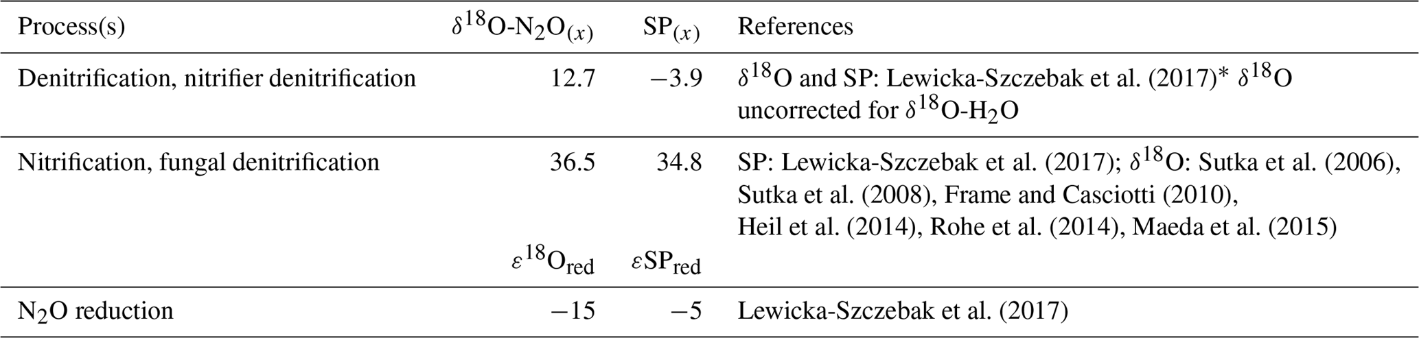
* Lewicka-Szczebak et al. (2017) originally report . Thus, to calculate a pure , we added the δ18O-H2O value used in our study (−8.3 ‰).
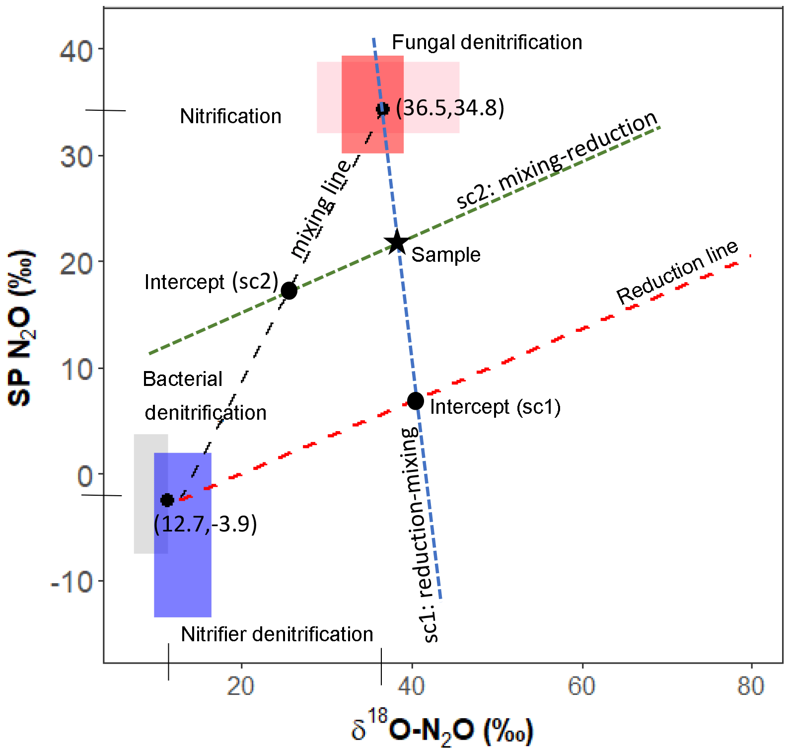
Figure 1Mapping approach scheme used in the closed-system modeling. Adapted from Lewicka-Szczebak et al. (2017).
Closed-system fractionation for N2O reduction was modeled following the method described in Lewicka-Szczebak et al. (2017) (Fig. 1). A detailed protocol for these calculations can also be found on ResearchGate (https://doi.org/10.13140/RG.2.2.17478.52804, last access: 15 January 2019). In brief, sample SP and δ18O-N2O values are used to derive sample-specific intercepts that pass through the sample and reduction line (sc1) or the sample and the mixing line (sc2). A fixed slope for the reduction line can be calculated from εSPred ∕ ε18Ored (i.e., in our case, ). In sc1, the intercept of the mixing and reduction line represents N2O that has been produced from denitrification/nitrifier denitrification and partially reduced but not yet mixed with N2O produced from nitrification/fungal denitrification. In sc2, the intercept of these lines represents N2O that has been produced by the two end-member pools, mixed but not yet reduced. The Y axis (i.e., SP) value of these respective intercepts can be used in a generalized Rayleigh equation (Eq. 4) to calculate the extent of N2O reduction, represented by the fraction of residual N2O not reduced.
In sc1 the rN2O is determined with respect to N2O from denitrification/nitrifier denitrification only; therefore, to calculate the residual fraction of total production (i.e., N2+N2O), we calculate gross rN2O:
To calculate the fraction of denitrification of the total initially produced N2O (emitted as N2O and N2), we calculate the gross denitrification fraction:
To calculate the fraction of denitrification/nitrifier denitrification to the net N2O produced, we use Eq. (7). For simplicity and comparison with open-system calculations, we call this DenContribution.
In this case, SPresid.N2O is the signature of residual bacterial N2O after partial reduction but before mixing. This was determined from the graphical method (Lewicka-Szczebak et al., 2017). In sc2 both net and gross fractions of denitrification are equal and can be expressed as
Here, SPN2O−undreduced is the signature of N2O mixed from nitrification/fungal denitrification and denitrification/nitrifier denitrification but before reduction. This was determined from the graphical method (Lewicka-Szczebak et al., 2017).
To predict rN2O in open systems, we set up a series of mass balance equations using our measured N2O flux or N2Oporeair concentrations and measured δ18O and SP values. We used the same end-member values listed in Table 2 for all equations. As above, we can model the interaction between mixing and reduction assuming sc1 (Eqs. 9–11) or sc2 (Eqs. 9, 12, 13). In Eqs. (9)–(13), we use knit, kden and kred to represent the gross process rates or concentrations of N2O attributable to nitrification, denitrification and N2O reduction, respectively.
These two sets of equations (Eq. 9, 10, 11) or (Eq. 9, 12, 13), representing each scenario, were applied to measured surface fluxes to produce process rates in g N2O-N ha−1 d−1 or were applied to N2Oporeair concentrations to produce concentrations of N2O in µg N2O-N L−1. By rearranging these process rates or concentrations, we can calculate gross rN2O, fracDEN and the contribution of denitrification to N2O using Eqs. (14)–(16).
Plausible solutions for kred, kden and kred were estimated based on minimizing the sum of squares between the modeled and measured N2O flux (or concentration), δ18O and SP values using a generalized reduced gradient (GRG) nonlinear algorithm in the Solver function of Excel. Example calculations for the open-system modeling are given in the Supplement. Solutions with a minimum sum of squares over 500 were considered implausible (8.3 % of solutions) (Table S2). Both models produced some non-plausible solutions, i.e., fractional contributions over 1 or under 0. Only solutions with a gross rN2O, gross fracDEN and DenContribution between 0 to 1 and an open-system minimum sum of squares < 500 were retained. In sc1, roughly 75 % of solutions met these criteria. For sc2, less than 10 % of solutions in the open system met this criterion; therefore, we did not proceed to analyze and discuss solutions from sc2 (Table S2 and Fig. S3).
2.8 Statistical analyses
Response variables were analyzed using a linear mixed effects analysis of covariance (ANCOVA) model with treatment, date and depth (if applicable) as fixed effects and plot as a random effect. The longitudinal position in the field (Y position) measured in meters from the central driveway (Fig. S2), was used as a covariate to account for potential heterogeneity in the longitudinal direction. In the case of non-normally distributed data, data were transformed to obtain a normal distribution of residuals. Due to the non-normal distribution of many variables, Spearman correlations were used to analyze the relationship between N2Oemitted fluxes, isotope ratios, and soil environmental and substrate variables. Post hoc analysis of treatment and depth within a given day was performed using the lsmeans function with a Tukey adjustment for multiple comparisons. For the analysis of modeling results we eliminated the 25 cm depth due to poor data availability. All data analysis was done in R version 3.3.2.
3.1 Yield
At the end of the growing season yield was measured in the larger plots in which sampling plots were situated. The DS-AWD treatment had a significantly lower yield, 6.6 t ha−1, relative to 8.9 and 8.2 t ha−1 in the WS-FLD and WS-AWD, respectively (Table 1).
3.2 N2O fluxes and dissolved and pore air N2O concentrations
3.2.1 Temporal patterns in N2O fluxes and concentrations
After the first basal fertilization (16 May) and prior to the second topdressing fertilization (21 June), emissions were significantly higher in the DS-AWD treatment than in WS-AWD and WS-FLD on 8 and 6 of the 11 sampling days, respectively (Fig. 2). During this time four peaks in emissions were observed in the DS-AWD treatment: on 20 May, 1–3, 7–9, and 20 June, averaging 39.5±5.1 g N2O-N ha−1 d−1. A peak in emissions following the second fertilization (21 June) was observed in all treatments; in the DS-AWD treatment, emissions peaked at 108.2±4.2 g N2O-N ha−1 d−1 on 23 June while in the WS-AWD and WS-FLD treatments, emissions peaked 1 day earlier reaching 49.4±17.9 and 77.67±10.6 g N2O-N ha−1 d−1, respectively. In the WS-AWD treatment, emissions remained slightly elevated following this fertilization until the end of the monitoring campaign, while in the DS-AWD and WS-FLD, emissions declined after 22 or 23 June, respectively.
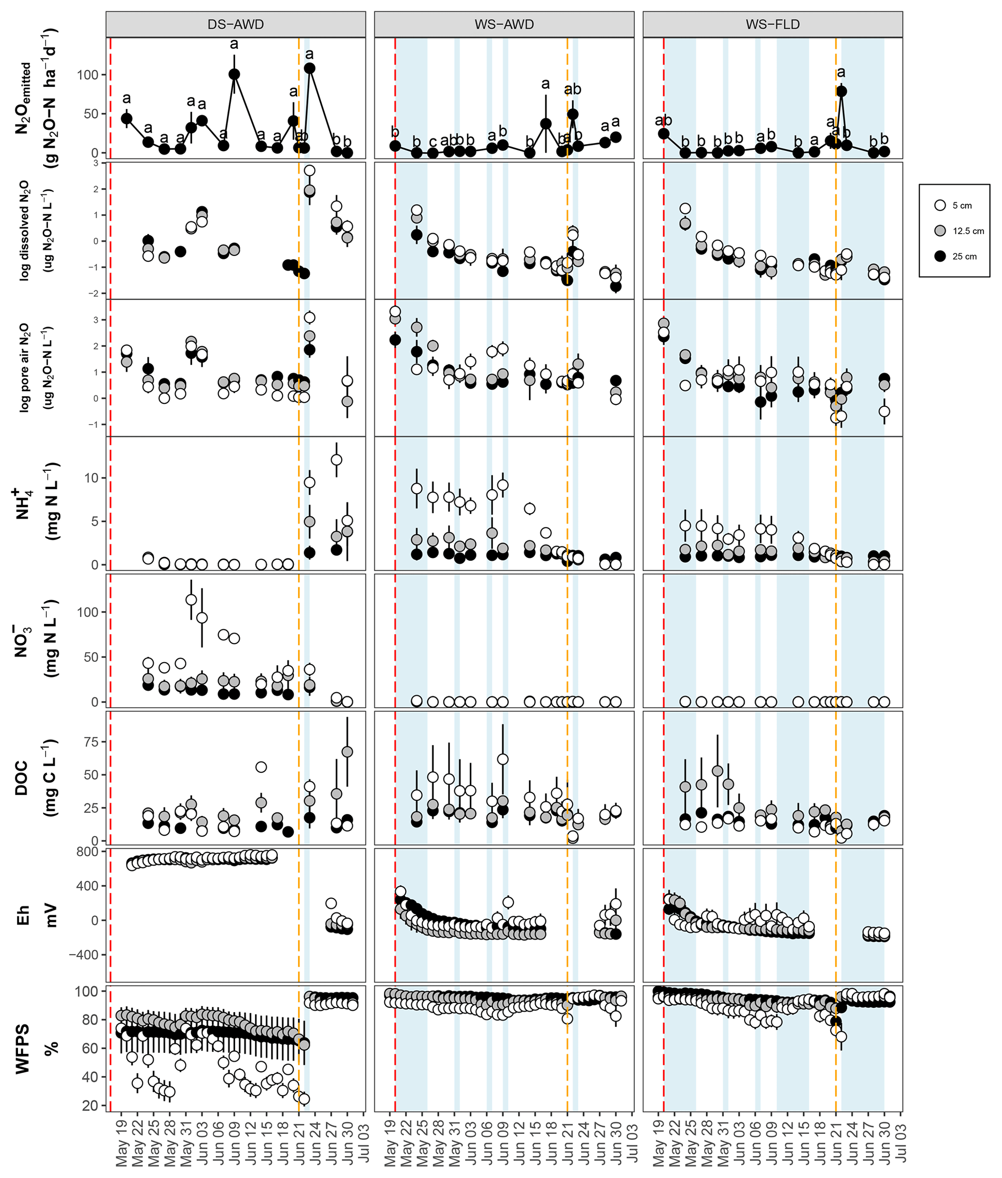
Figure 2N2O surface emissions, log10 of dissolved and pore air N2O concentrations, , , DOC, Eh, and WFPS throughout the field measurement period in the three water management treatments (WS-FLD: water-seeding + conventional flooding; WS-AWD: water-seeding + alternate wetting and drying; DS-AWD: direct dry seeding + alternate wetting and drying). The dashed vertical line indicates the date of fertilization (60 kg urea-N ha−1). Blue shaded areas represent periods of flooding; shaded areas that last only 1 day indicate “flush irrigation”, i.e., flooding for < 6 h. The error bars represent the standard error of the mean. Red and orange dashed vertical lines represent the date of seeding and fertilization in each treatment, respectively.
If we exclude N2Odissolved measurements from the DS-AWD treatment following the second fertilization (i.e., after the 22 June, when concentrations reached as high as 594.4±112.6 µg N2O-N L−1 at 5 cm), concentrations throughout the profile of all treatments remained under 20 µg N2O-N L−1. Due to the large differences between dates and treatments, we present the concentrations on a log10 scale (Fig. 2) and a non-transformed scale (Fig. S4). Peak concentrations in the WS treatments occurred at 5 cm on the first day of measurement, reaching 17.7±5.1 and 18.5±2.8 µg N2O-N L−1 in the WS-AWD and WS-FLD, respectively. In comparison, in the DS-AWD treatment, peak concentrations prior to the second fertilization were observed at 25 cm on 3 June, reaching 18.5±8.3 µg N2O-N L−1.
As with dissolved N2O, pore air N2O concentrations were highly variable between treatments and between sampling days and are again presented on a log10 scale (Fig. 2) and non-transformed scale (Fig. S4). In both WS treatments, the highest concentrations were observed on the first day of measurement, 20 May, reaching 2903.3±1103.6 and 1321±998.0 µg N2O-N L−1 at 5 cm in the WS-FLD and WS-AWD, respectively. Elevated concentrations of N2Oporeair were also observed in the DS-AWD on the first day of measurement but were 70.1 µg N2O-N L−1 at 5 cm (roughly 40× lower than in WS-FLD on this date). Maximum concentrations in the DS-AWD treatment were observed 2 days after the second fertilizer application, reaching 1902.2 µg N2O-N L−1; in contrast, no change was observed in the WS treatments following this fertilizer application. In all treatments the majority of N2Oporeair concentrations were orders of magnitude lower than these peaks. There was a tendency of lower N2Oporeair concentrations in the DS-AWD treatment relative to the WS treatments; this pattern was most evident at 5 cm (Fig. 2). However, treatment differences in N2Oporeair were not significant (p=0.08, Table S3), and there was a significant date × treatment interaction.
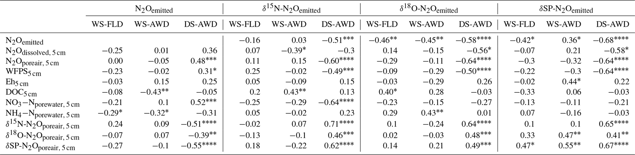
Table 3Spearman correlations of N2Oemitted with N2Oemitted isotope ratios, N2O driving variables and N2Oporeair isotope ratios measured at 5 cm in the three water management treatments (WS-FLD: water-seeding + conventional flooding; WS-AWD: water-seeding + alternate wetting and drying; DS-AWD: direct dry seeding + alternate wetting and drying). Significance indicated by < 0.0001, < 0.001, < 0.01, * < 0.05.
3.2.2 Relation of N2O fluxes and concentrations with soil environment, substrates and N2O isotope ratios
We evaluated the correlation of N2Oemitted with Eh, WFPS, , , dissolved and pore air N2O concentrations, and N2O isotope ratios at 5 cm (Table 3). Among these variables, N2O emissions in the WS treatments were negatively correlated with pore water and DOC in the WS-AWD treatment. In the DS-AWD treatment, emissions positively correlated with N2Oporeair, WFPS and and negatively with N2O isotope ratios. Examining the isotope ratios of N2Oemitted, we observed that N2Oemitted was negatively correlated with δ18O-N2Oemitted in all treatments, negatively with δ15N-N2Oemitted in the DS-AWD treatment, and negatively with SP-N2Oemitted in the WS-FLD and DS-AWD. Interestingly, a positive correlation between N2Oemitted and SP-N2Oemitted was observed in the WS-AWD treatment. Relative to the DS-AWD, the WS treatments had fewer significant correlations between N2O isotope ratios, soil environment or pore air N2O isotope ratios. DOC was positively correlated with δ15N-N2Oemitted in the WS-AWD and with δ18O-N2Oemitted in the WS-FLD. SP-N2Oemitted was positively correlated to Eh and negatively to WFPS in the WS-AWD treatment. In comparison, in the DS-AWD treatment, N2Oemitted isotope ratios were positively correlated to that of N2Oporeair for all three isotopes. Furthermore, N2O isotope ratios in the DS-AWD treatment were negatively correlated with N2Oporeair concentrations, WFPS, (δ15N-N2Oemitted only) and N2Odissolved (δ18O-N2Oemitted and SP-N2Oemitted only). It should be noted that N2Odissolved in the DS-AWD treatment was not measurable at the 5 cm depth in 10 of the 16 sampling dates due to low soil moisture and low pore water volumes.
3.3 Spatiotemporal patterns of N2O isotope ratios
3.3.1 δ15N-N2O
A consistent temporal pattern of higher N2Oporeair concentrations and N2Oemitted fluxes in association with lower δ15N was observed in the DS-AWD treatment. In the WS treatments, high N2Oemitted fluxes on 23 June following the second fertilization were associated with lower δ15N (Fig. 3); this was not the case for a high flux in the WS-AWD on 17 June. N2Oporeair at 5 cm in the WS-AWD treatment tended to be higher in concentration and lower in δ15N relative to other depths; however, in general a consistent relationship between concentration and δ15N was less evident in the two WS treatments. On average, the δ15N of N2Oemitted was lower relative to N2Oporeair in the DS-AWD treatment. In contrast, in the WS treatments N2Oemitted was depleted in 15N relative to N2Oporeair at all depths only immediately before and after the second fertilization. In these treatments, δ15N-N2Oporeair was generally lower at 5 cm relative the other depths but tended to increase and reach similar values as the other depths over the experimental period. As a result, N2Oemitted was often enriched in 15N relative to N2Oporeair at 5 cm in these treatments, particularly in the WS-AWD treatment.
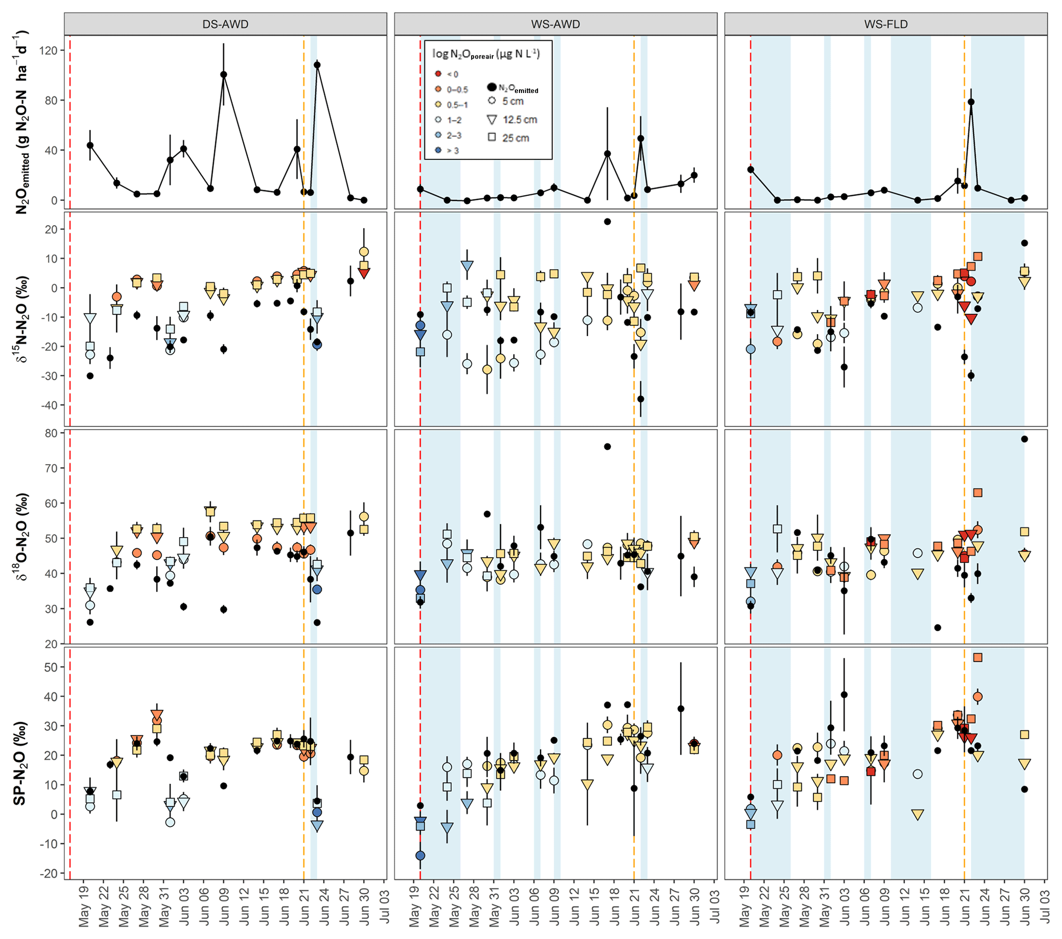
Figure 3Time course of δ15N-N2O, δ18O-N2O and SP-N2O in N2Oemitted and N2Oporeair across the three depths and water management treatments (WS-FLD: water-seeding + conventional flooding; WS-AWD: water-seeding + alternate wetting and drying; DS-AWD: direct dry seeding + alternate wetting and drying). The error bars represent the standard error of the mean. Red and orange dashed vertical lines represent the date of seeding and fertilization in each treatment, respectively.
3.3.2 δ18O-N2O
As with δ15N, δ18O isotope ratios spanned a large range, particularly in the emitted N2O (Fig. 3). δ18O-N2Oporeair in the DS-AWD followed a temporal pattern similar to δ15N,s and similarly, δ18O was generally lower in N2Oemitted relative to N2Oporeair. The highest δ18O-N2Oporeair was seen in the DS-AWD treatment at moderate N2Oporeair concentrations where δ18O isotope ratios were higher than other concentrations in the DS-AWD or any concentration in the WS treatments. These samples were also nearly always taken from 12.5 or 25 cm. In all treatments, lower δ18O values were observed in N2Oporeair and N2Oemitted on the first day of sampling: global mean of 35.1±1.1 and 29.6±1.7 ‰ relative to 46.9±0.4 and 43.9±1.7 ‰, respectively. Otherwise, no distinct pattern with depth, time or concentration was observed in the WS treatments.
3.3.3 SP-N2O
The SP of N2Oemitted ranged from 4.5±0.4 ‰ to 25.6±8.1 ‰, from 2.9±1.0 ‰ to 37.2 ‰ (un-replicated) and from 5.8±0.6 ‰ to 40.6±12.4 ‰, in the DS-AWD, WS-AWD and WS-FLD treatments, respectively (Fig. 3). In contrast to δ15N and δ18O isotope ratios, the SP-N2Oporeair tended to increase with time but only in the WS treatments. As with δ15N-N2O and δ18O-N2O, moderate- and lower-concentration N2Oporeair samples showed higher SP values relative to higher-concentration N2Oporeair samples. For example, 2 days after the second fertilizer application (23 June), SP values decreased in conjunction with increased N2Oporeair concentrations in the DS-AWD treatment. On this date, mean SP values at 5 cm demonstrated the largest treatment differences with values of 0.7±4.5 ‰, 27.6±2.1 ‰ and 39.9±2.7 ‰ in the DS-AWD, WS-AWD and WS-FLD treatments, respectively. On this date, the pattern between the treatments was consistent throughout the three depths.
3.3.4 Relationships between N2O isotope ratios
Considering all depths and emitted data together, δ18O-N2O significantly and positively correlated with δ15N-N2O and SP across all treatments. The slope of δ18O-N2O vs. δ15N-N2O was 0.67, 0.28 and 0.52 (Fig. S5) and 0.67, 0.54 and 0.31 for SP vs. δ18O-N2O in the DS-AWD, WS-AWD and WS-FLD treatments, respectively (Fig. 4a). There was no correlation between SP and δ15N-N2O in the two WS treatments, but a positive correlation for the DS-AWD was found, with a slope of 0.62 (Fig. 4b). Examining these relationships by depth, we saw the strongest relationship and highest slope in the N2Oemitted and at 25 cm for δ18O-N2O vs. δ15N-N2O (Fig. S5). While the SP vs. δ18O-N2O showed no correlation among the surface fluxes in the WS treatments, the two isotope ratios were positively correlated in N2Oporeair at all depths and treatments (Fig. S6). A contrasting relationship between SP and δ15N-N2O was observed for the WS-FLD treatment in the N2Oemitted and N2Oporeair where the two isotope ratios were negatively correlated in N2Oemitted and positively in N2Oporeair (Fig. S7).
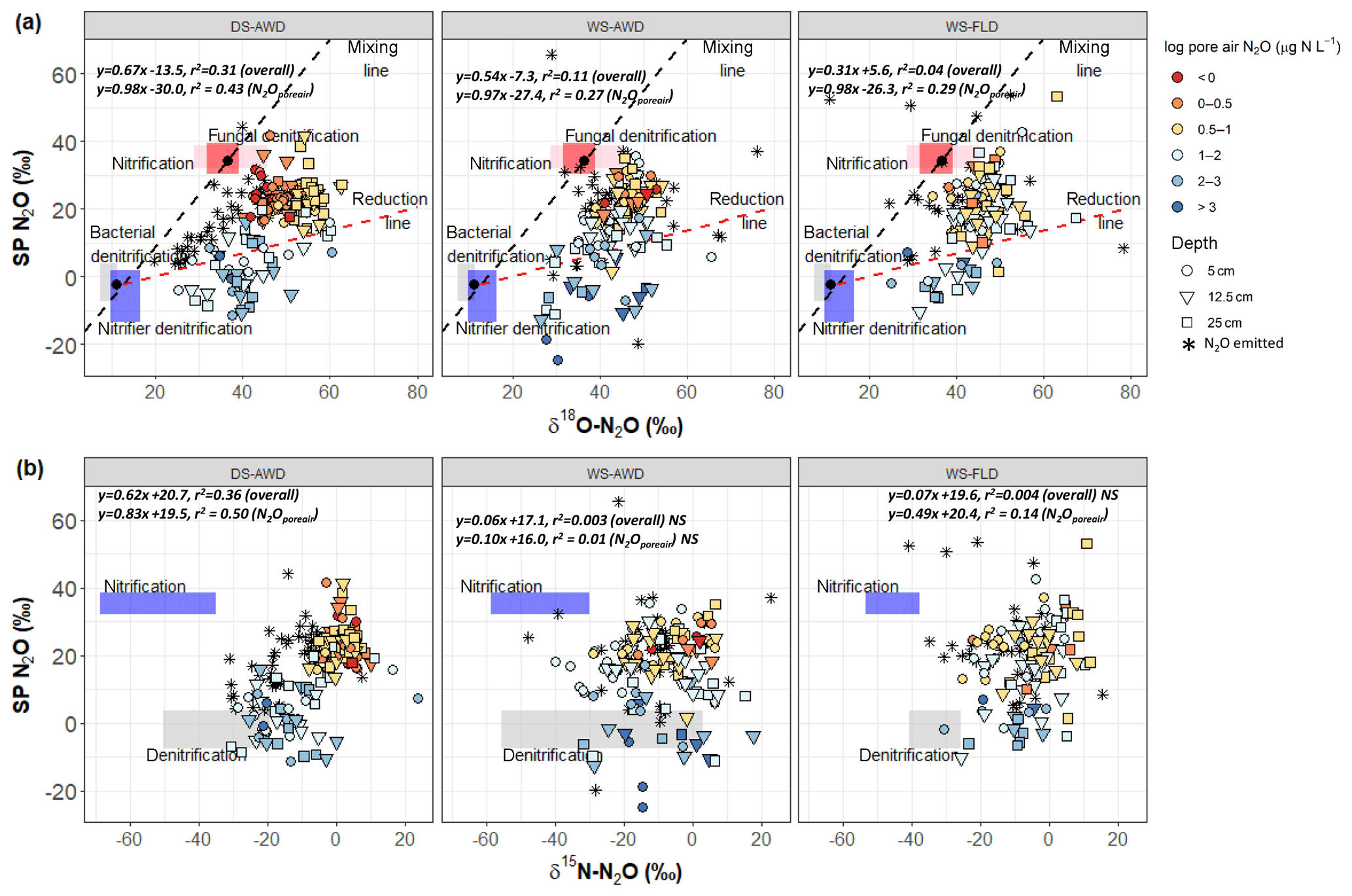
Figure 4Graphical two end-member mixing plot after Lewicka-Szczebak et al. (2017) where sample values are plotted in SP × δ18O−N2O space A and two-end mixing plot after Toyoda et al. (2011) where sample values are plotted in SP × δ15N-N2O space B. In panel (a) the black dots indicate the mean literature end-member values used in our modeling scenarios and the boxes represent a range of values derived from the literature attributed to each process; see Sect. 2.7 and Table 2. To calculate the range of N2O potentially produced by nitrification or denitrification in (b), we used the mean isotope effects, and , reported in Denk et al. (2017) to represent denitrification and nitrification derived N2O, respectively, and then added the minimum and maximum δ15N- and δ15N- values observed in each treatment (Table S1.4). The linear relationship between each isotope pair is indicated in italics for all points together and for N2Oporeair only. The three water management treatments were as follows: WS-FLD – water-seeding + conventional flooding; WS-AWD – water-seeding + alternate wetting and drying; DS-AWD – direct dry seeding + alternate wetting and drying.
3.4 and concentrations and isotope ratios
3.4.1 Spatiotemporal trend in and concentration and δ15N and δ18O isotope ratios
In all treatments, pore water concentrations were highest at 5 cm relative to the other depths (Fig. 2). In the DS-AWD treatment concentrations were almost zero prior to the second fertilization, remaining below 0.85 mg -N L−1 across all depths. Following this fertilization, concentrations increased at all depths, most notably at 5 cm. An opposing pattern was observed in the WS treatments where was nearly always significantly higher than in DS-AWD for each corresponding depth leading up to the second fertilization but dropped to near zero following the fertilization. Nitrate concentrations were exclusively less than 1.5 mg NO3-N L−1 in both WS treatments throughout the experimental period. In sharp contrast, concentrations in the DS-AWD were at times more than 75 times higher than in WS treatments, peaking on 1 June at 113.6±22.4 mg NO3-N L−1. Following this spike, concentrations steadily declined and dropped to zero following the second fertilization.
3.4.2 δ15N-, δ15N- and isotope enrichment factors: and
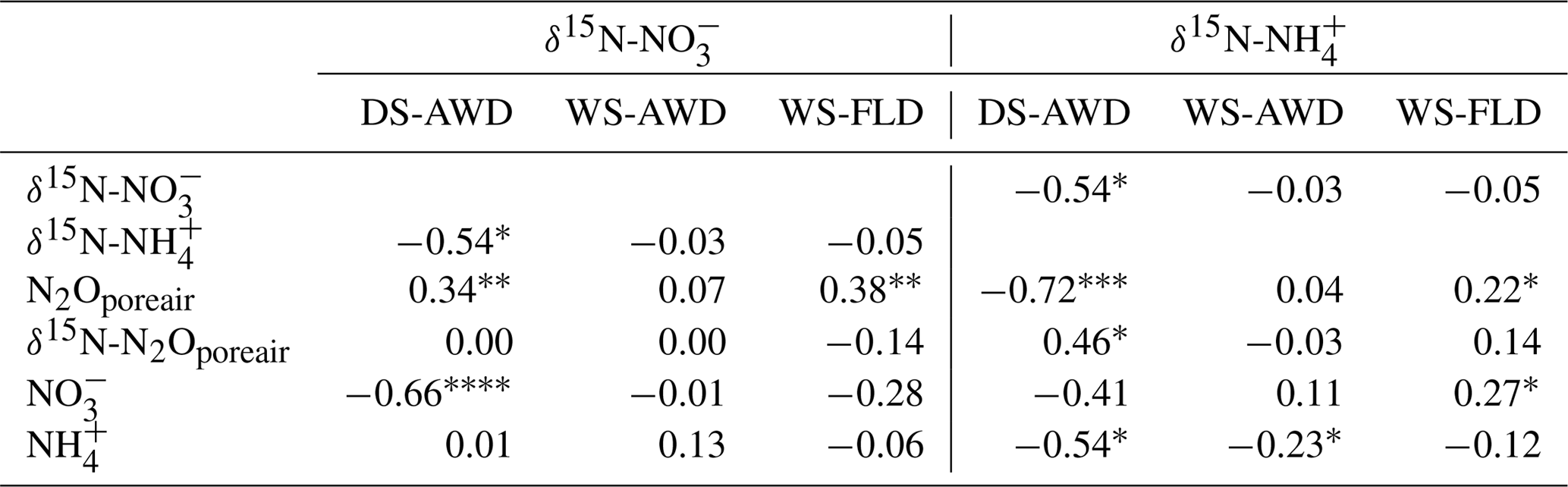
Concentrations of or were often too low for isotope measurements. Hence, we could only obtain sufficient replication for statistical analysis across depths and treatments on 5 days for (24 and 27 May; 1, 14 and 23 June) and 2 days for (24 May and 23 June) (Fig. S9). Daily mean δ15N- ranged from −4.3 ‰ to 28.3 ‰ across all treatments and depths. In the DS-AWD treatment a consistent depth pattern was observed with 15N enrichment of at 25 cm > 12.5 cm = 5 cm. δ15N- increased with time at 5 cm, rising from ‰ to 22.0±4.9 ‰. Significant treatment and depth differences were observed on 24 and 27 May and 1 June, but no differences were observed on later dates (14 or 23 June). Following the second fertilizer application, δ15N- values in the DS-AWD treatment rose by approximately 10 ‰ at all depths. Daily mean δ15N- ranged from −6 ‰ to 15.2 ‰ (Fig. S9). Averaging across the experimental period and depths, mean δ15N values of and were similar (8.4 ‰ and 7.0 ‰, respectively; Table S5). There was no evident temporal or depth trend in δ15N- in any of the treatments. The only significant difference was lower δ15N- in the DS-AWD on 23 June. δ15N- values positively correlated to N2Oporeair concentrations in the DS-AWD and WS-FLD treatments and were negatively correlated to concentrations and to δ15N- in the DS-AWD treatment (Table 4). δ15N- was negatively correlated to N2Oporeair concentrations and concentrations and positively to δ15N-N2Oporeair in the DS-AWD treatment.
Table 4Spearman correlations between δ15N- and δ15N- with N2Oporeair concentration, δ15N-N2Oporeair, and concentrations in the three water management treatments (WS-FLD: water-seeding + conventional flooding; WS-AWD: water-seeding + alternate wetting and drying; DS-AWD: direct dry seeding + alternate wetting and drying).
Largely reflecting the depth pattern of δ15N- in the DS-AWD, the calculated tended to be highest at 5 cm, with a mean of ‰, while mean values at 12.5 and 25 cm were slightly lower ( and ‰, respectively; Fig. S9). At 5 cm values in the DS-AWD were significantly higher than in the WS treatments; at 12.5 cm they tended to be higher as well but the difference was not significant. Two days after the second fertilizer application, the in the DS-AWD markedly decreased at all depths to a treatment mean of ‰. In comparison, WS treatment values rose 1 (WS-FLD) or 2 (WS-AWD) days following the fertilization. In the WS-FLD, the increase in values lasted only 1 day; unfortunately, low concentrations precluded δ15N- analysis on many dates making temporal patterns difficult to observe. Mean depths by treatment isotope effects calculated relative to δ15N- () were ‰, ‰ and ‰ at 5 cm; ‰, ‰ and ‰ at 12.5 cm; ‰, ‰ and ‰ at 25 cm for DS-AWD, WS-AWD and WS-FLD treatments, respectively. Data for was scarce in the DS-AWD treatment due to low concentrations; in the WS treatments increased with depth, but these differences were not significant.
δ18O- was significantly depleted in the DS-AWD treatment relative to both WS treatments (Fig. S9). Prior to the second fertilization, values were remarkably consistent in the DS-AWD at all depths, ranging from 0.1 ‰ to 7.5 ‰. Two days after this fertilizer application, δ18O- rose to a mean of 7.6 ‰ across depths. In comparison the of both WS treatments was more variable between sampling dates, fluctuating between 12.2 ‰ and 38.8 ‰ and 10.4 ‰ and 32.7 ‰ leading up the second fertilization in the WS-AWD and WS-FLD, respectively. Two days after the second fertilizer application values rose to a mean of 23.7 ‰ and 27.4 ‰ across depths in the WS-AWD and WS-FLD, respectively. We calculated the net isotope effect for δ18O-N2O relative to water (). The in all treatments and depths tended to rise over the course of the measurement period, with the most consistent rise observed at 5 cm. Here values rose from a global mean of 43.8±1.0 ‰ on 20 May to 58.5±1.0 ‰ on 30 June. There was a pattern of higher in the DS-AWD treatment relative to the two WS treatments. A drop in of ∼10 ‰ was observed in all depths on 23 June, 2 days after the second fertilization with urea, in the DS-AWD only.
3.5 SP × δ18O-N2O two end-member mixing model to estimate N2O reduction, source contributions and N2O reduction
To further quantitatively interpret our isotope ratio data, we employed a graphical two end-member mixing model (Lewicka-Szczebak et al., 2017), based on the relationship between SP and δ18O-N2O (Figs. 1 and 4). Data were modeled for open and closed fractionation dynamics under two scenarios. In sc1, reduction of N2O from the denitrification/nitrifier-denitrification end-member pool occurs prior to mixing with nitrification/fungal denitrification-derived N2O; in sc2, mixing of N2O from both end-member pools occurs before reduction. For sc2, our model yielded implausible results for the contribution of denitrification/nitrifier denitrification to N2O emissions in about 90 % and 20 % of observations under open- and closed-system dynamics, respectively (Table S2). The poorer outcomes from sc2 in the open system indicate that the assumptions underlying this scenario are likely false in open systems or vice versa. In order to have comparable data between open and closed systems, we discuss only results coming from sc1 simulations.
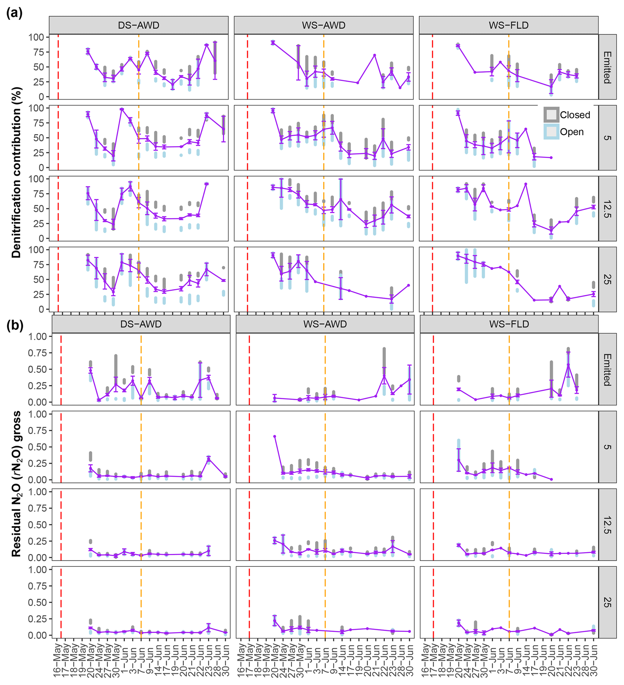
Figure 5Modeled denitrification/nitrifier-denitrification contribution and gross rN2O of open (grey bars), closed (blue bars) and mean (purple points and line) systems predicted by a two end-member mixing model using δ18O-N2O and SP values. For open- and closed-system dynamics, the shaded bars represent the standard deviation range for each treatment × depth combination. The purple error bars represent the standard deviation around the mean. Red and orange dashed vertical lines represent the date of seeding and fertilization in each treatment, respectively.
Temporal trends in the gross rates of rN2O (extent of N2O reduction) predicted by open- and closed-system N2O fractionation were nearly identical (Fig. 5b). Gross rN2O was estimated to be higher (i.e., lower N2O reduction) under closed-system fractionation dynamics. In reality, it can be assumed that neither perfect open or closed systems exist in nature and processes likely reflect a mixture of these dynamics. The use of one or the other case may bias results; therefore, we chose to take the mean of the two systems to estimate N2O reduction, nitrification/fungal denitrification and denitrification/nitrifier denitrification-derived N2O emissions (Decock and Six, 2013b; Wu et al., 2016). Due to a disproportionate number of missing values at 25 cm in the two WS treatments, we chose not to include data from this depth in our analysis and discussion. Therefore, further values refer to the mean of open and closed systems and N2Oemitted or N2Oporeair at 5 cm and 12.5 cm unless explicitly stated otherwise. Gross rN2O fractions tended to be higher in N2Oemitted (treatment means 0.14 to 0.19) relative to the subsurface (treatment means 0.06 to 0.15). While water management treatment had a significant effect on process contributions to N2Oemitted and N2Oporeair (Table 5), significant interactions with depth and date were observed. Gross rN2O fractions in N2Oporeair were significantly lower in the DS-AWD relative to the WS-FLD on 6 of 15 days, with the WS-AWD falling in between. In the N2Oemitted, the opposite pattern was mostly observed with gross rN2O fractions often being higher in the DS-AWD than one or the other WS treatments, significantly so on 4 of 15 days. Aggregated across depths, the contribution of denitrification/nitrifier denitrification to N2Oporeair were higher in the DS-AWD relative to one or both WS treatments on four dates and lower on three dates (Fig. 5a). The mean contribution of denitrification/nitrifier denitrification to N2Oemitted ranged from 43 % to 49 % in all treatments (Fig. 6). Denitrification/nitrifier-denitrification contributions to N2Oemitted were higher in the DS-AWD relative to the WS treatments on 9 and 23 June, and relative to WS-AWD only, they were also higher on 28 June and lower on 21 June.
Table 5P-value ANCOVA results of modeled residual N2O not reduced (gross rN2O), fraction of total N2+N2O production coming from denitrification (gross fracDEN), and the fraction of N2O attributed to denitrification (DenContribution) derived from N2Oemitted and N2Oporeair. The Y position was used a covariate and represents the longitudinal position of each replicate within the field. Numbers in bold indicate significance at p < 0.05.

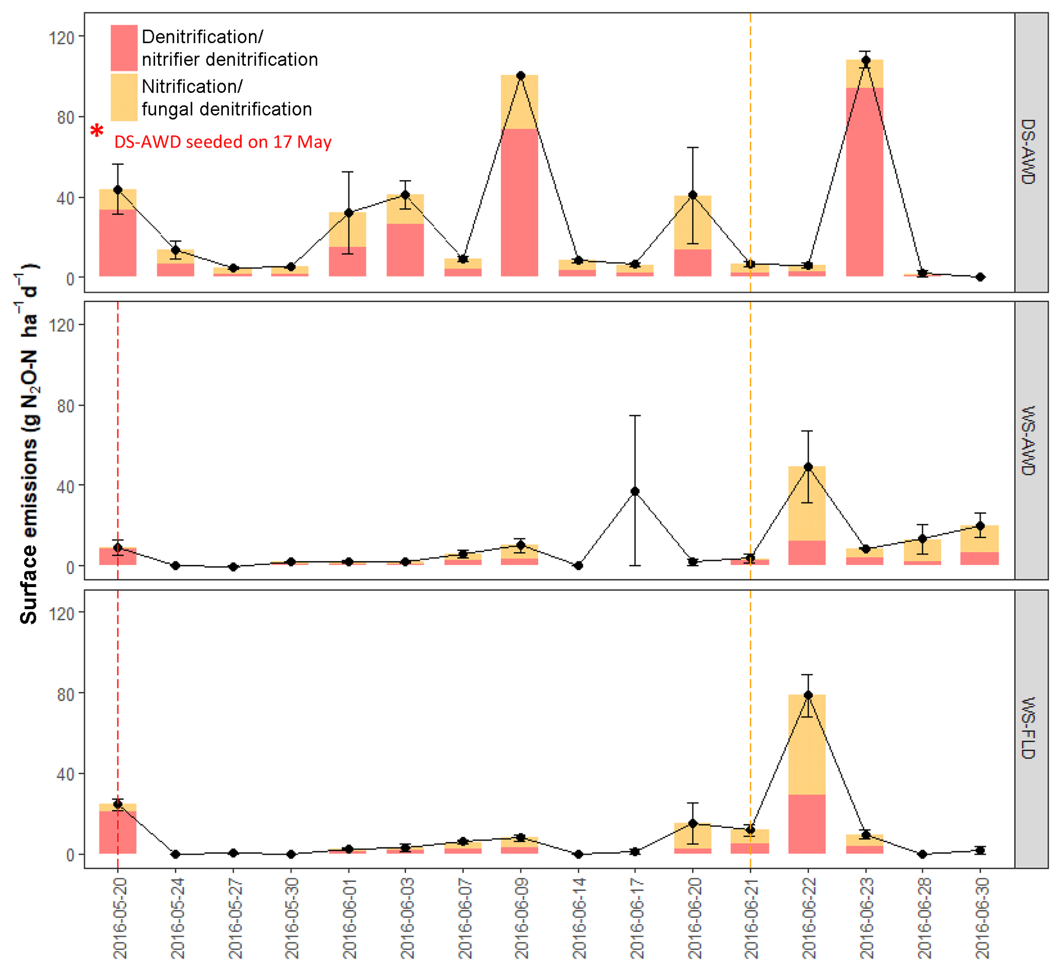
Figure 6Estimated contribution of denitrification/nitrifier denitrification and nitrification/fungal denitrification to N2O surface emissions in the three water management treatments (WS-FLD: water-seeding + conventional flooding; WS-AWD: water-seeding + alternate wetting and drying; DS-AWD: direct dry seeding + alternate wetting and drying). Estimates were derived from the mean of open and closed dynamics in a two end-member mixing model using δ18O-N2O and SP values. Red and orange dashed vertical lines represent the date of seeding and fertilization in each treatment, respectively.
4.1 Patterns of N2Oemitted, N2Oporeair and N2O isotope ratios
In accordance with results from past studies (Miniotti et al., 2016; Peyron et al., 2016; Cai et al., 1997) and in line with our hypothesis, we observed higher N2O emissions on most days in the DS-AWD relative to the two WS treatments (Fig. 2). A belated divergence in water management between the WS-FLD and WS-AWD (Table 1), in addition to a relatively wet early summer, likely contributed to similar observed soil environmental conditions and N substrates among these two treatments. Therefore, given the similarities in soil conditions, it is not surprising that N2O fluxes and isotope ratio differences between these two treatments were generally fewer than expected. The lower yield in the DS-AWD treatment likely contributed additional differences in pore water N concentrations because lower N demand in this treatment should have resulted in higher soil N concentrations.
Mean daily δ15N, δ18O and SP values of N2Oemitted and N2Oporeair per depth and treatment ranged from −27.9 ‰ to 12.3 ‰, 30.9 ‰ to 63.0 ‰ and −14.0 ‰ to 53.2 ‰, respectively (Fig. 3). These values are similar in magnitude to those observed by Yano et al. (2014) in the early growing season of rice, where ranges of −24 ‰ to 6 ‰, 24 ‰ to 66 ‰ and 4 ‰ to 25 ‰ were reported. Our values are also similar in magnitude to those observed in other field studies which have included depth sampling (Koehler et al., 2012; Zou et al., 2014). Relative to these two studies we observed higher δ15N-N2O and both higher and lower SP ratios. This was likely due to a higher sampling frequency, which covered more variable soil environments and generally higher soil moisture in our study than in the others. For example, it has been shown that organic matter decomposition and DOC availability in rice systems can decline with the introduction of wet–dry cycles or dry seeding (Said-Pullicino et al., 2016; Yao et al., 2011); thus, it is likely that conditions promoting complete denitrification declined in the AWD treatments. In contrast, saturated conditions favoring complete denitrification certainly prevailed in the WS treatments at times. Working in a denitrifying aquifer, Well et al. (2012) observed very large ranges in δ15N and SP ratios, varying from −55.4 ‰ to 89.4 ‰ and 1.8 ‰ to 97.9 ‰, respectively.
4.2 Source-partitioning N2O production
One method to source partition emissions is to calculate net isotope effects and compare these to literature values derived from controlled and pure culture experiments where isotope effects were determined for individual processes. The calculated in the DS-AWD treatment, with depth means of −7.2 ‰ to −16.0 ‰, was consistently much higher (i.e., less strong fractionation) than literature values reported for denitrification of (mean: ‰; Denk et al., 2017) (Fig. S9). At 5 cm in the two WS treatments, the mean was lower than in the DS-AWD (−23.2 and −21.5 in the WS-AWD and WS-FLD, respectively) but still nearly 20 ‰ higher than literature values. In a rice system, Yano et al. (2014) observed an of −6.7 ‰, very well within the range of our calculated . Similarly, the global mean of our values was −14.8 ‰, thus on average much higher than those reported in the literature for nitrification (−46.9 ‰, Sutka et al., 2006; ‰, Denk et al., 2017). For both isotope effects, similar scenarios may explain our high observed Δ15Nx (i.e., low fractionation), namely, (i) non-steady-state reactions, for example rapid refreshing of the and pools or near-complete substrate consumption, or (ii) significant reduction of N2O serving to increase δ15N-N2O values and thereby reducing the net isotope effect.
Considering the moist conditions and high reduction rates, it seems most likely that strong N2O reduction was the largest contributor to the greater degree of isotopic discrimination observed. To check this, we estimated initial δ15N-N2O values before N2O reduction using our modeled N2O reduction fraction (rN2O), measured δ15N-N2O values and an 15N isotope effect during reduction of −6.6 ‰ (Denk et al., 2017) in the Rayleigh equation. We could then estimate amended values if N2O reduction effects were accounted for from the difference between our initial δ15N-N2O estimates and δ15N-. These calculations yielded a from −25.0 ‰ to −36.5 ‰, −32.6 ‰ to −42.3 ‰ and −29.0 ‰ to −51.1 ‰ in the DS-AWD, WS-AWD and WS-FLD across depths (Table S6). These amended values do decrease and, especially for the WS treatments, come relatively close to literature values for during denitrification. Thus, significant N2O reduction can likely explain much of the high values observed, particularly in the WS treatments. Yet other factors were also likely at play to some degree. For example, in the DS-AWD, where we observed evidence of significant nitrification, it is quite possible to envision isolated enrichment of at anaerobic micro-sites where N2O is produced, while the bulk soil pool remained less enriched. It is also true that we could not always measure δ15N values of or because the concentrations were too low; thus, we could not calculate isotope effects. This highlights a persistent dilemma, which is true for all isotope ratios, that we cannot accurately measure isotope ratios at very low concentrations. Hence, until more sensitive methodologies are developed, in situ measurements such as these will always be biased toward higher-concentration scenarios where perhaps the strongest and most interesting effects of substrate enrichment are missed.
The use of any one isotope signature alone is confounded by overlap in the isotope effects between processes, unknown and possibly rapidly changing substrate δ values, and the unknown contribution of N2O reduction effects. To overcome these drawbacks, graphical interpretations of dual N2O isotope ratios have been used in field studies to interpret datasets similar to ours (Well et al., 2012; Koehler et al., 2012). For a more quantitative assessment of source partitioning, mixing models using a dual isotope approach can be used (Yano et al., 2014; Toyoda et al., 2011; Koba et al., 2009; Lewicka-Szczebak et al., 2017; Zou et al., 2014). In the subsequent analysis, we employ both approaches using our sample values plotted in SP × δ18O and SP × δ15N space (Figs. 4 and S10–S12).
In both SP × δ18O and SP × δ15N plots, our sample values mostly fell between the mixing and reduction lines predicted by either isotope relationship (Fig. 4) and somewhat surprisingly showed stronger enrichment, indicative of greater N2O reduction in the DS-AWD treatment relative to the WS treatments. In the DS-AWD and to a lesser extent in the WS-AWD treatment, high pore air N2O concentrations were associated with denitrification or nitrifier denitrification, while midrange concentrations were associated with a higher degree of N2O reduction and the lowest concentrations fell neatly in between. Similarly, in the WS-FLD treatment, denitrification or nitrifier denitrification associated samples almost exclusively coincided with high N2Oporeair. Most likely the moderate N2Oporeair concentrations derived from N2O reduction following high denitrification/nitrifier-denitrification production. This analysis is supported by data showing a trend of enrichment over the course of the measurement period (Fig. S10) and high WFPS values associated with the most enriched N2Oporeair in the DS-AWD (Fig. S12). All treatments showed an enrichment of SP with time (Fig. S10), but interestingly only in the DS-AWD did δ18O and δ15N-N2O enrich over the course of the experiment. This may reflect an increase over time in δ15N and δ18O of , which was observed in the DS-AWD treatment, albeit not strongly (Fig. S9). More was available for denitrification in the DS-AWD treatment; thus, for greater enrichment of this pool to occur, we propose that more was trapped in denitrifying micro-sites as the soil dried or O2 was consumed.
In the WS treatments we observed a minimized trend of N2O reduction compared to the DS-AWD treatment, more scattered high SP values and more values intermediate to the two end-member pools. These results may partially be explained by greater contributions from abiotic hydroxylamine decomposition (SP ∼34 ‰–35 ‰; Heil et al., 2014) or fungal denitrification (SP ∼35 ‰; Rohe et al., 2014). Zhou et al. (2001) showed that fungal denitrification requires minimal oxygen to proceed; similarly Seo and DeLaune (2010) found that fungal denitrification dominated relative to bacterial denitrification at modest reducing conditions to weakly oxidizing conditions (Eh > 250 mV). Indeed, there is some evidence that high scattered SP values corresponded to more moderate WFPS (70 %–90 %) in the WS-FLD treatment (Fig. S12). Abiotic hydroxylamine decomposition requires nitrification for the production of NH2OH and iron or manganese (hyrdr)oxides as electron acceptors to proceed (Bremner et al., 1980). Given the moist conditions, nitrification rates were likely low in the WS treatments. Feasible co-occurrence of these species could really only occur directly in the rhizosphere of a flooded rice soil, where O2 is transported to the immediate root zone by the aerenchyma. Tightly coupled nitrification–denitrification in the rhizosphere of rice plants has been shown before (Arth and Frenzel, 2000) as has coupling of nitrogen–iron transformations (Ratering and Schnell, 2000), but we cannot say the extent to which this may have occurred in our system.
It is necessary to contextualize N2O isotope data with our measured substrate concentrations and soil environmental data. Based on our observations of low concentrations, high concentrations, an Eh over 400 mV and WFPS often below 60 % (5 cm) or below 85 % (12.5 and 25 cm) in the DS-AWD treatment, we can safely deduce that extensive nitrification of either basal urea fertilizer or of indigenous soil N occurred in this treatment (Fig. 2). Furthermore, the δ18O- in the DS-AWD treatment ranged from 0.1 to 14.8 (Fig. 7), thus falling in the range attributed to produced from nitrification (Kendall and McDonnell, 1998). Additionally, we observed that both δ15N- and δ15N- were negatively correlated to substrate concentrations in the DS-AWD treatment, indicative of active consumption of both N substrates (Table 4). In the DS-AWD, there also was a positive correlation between δ15N- and N2Oporeair but a negative correlation between δ15N- and N2Oporeair. The former likely indicates N2O production via denitrification and subsequent enrichment of the pool. The latter is more difficult to interpret, but we attributed this to higher emissions associated with fresh inputs of (from urea or mineralization) which should have a δ15N value around 0 ‰. Together these data show that coupled nitrification–denitrification was responsible for the majority of N2O emissions. Similar results were also reported by Dong et al. (2012) for an AWD system. The separation of isotope ratios by date, N2O concentration and WFPS suggests that produced early in the growing season was progressively denitrified and reduced over the course of the sampling period. Similarly, N2O produced early in the growing season may have been progressively reduced.
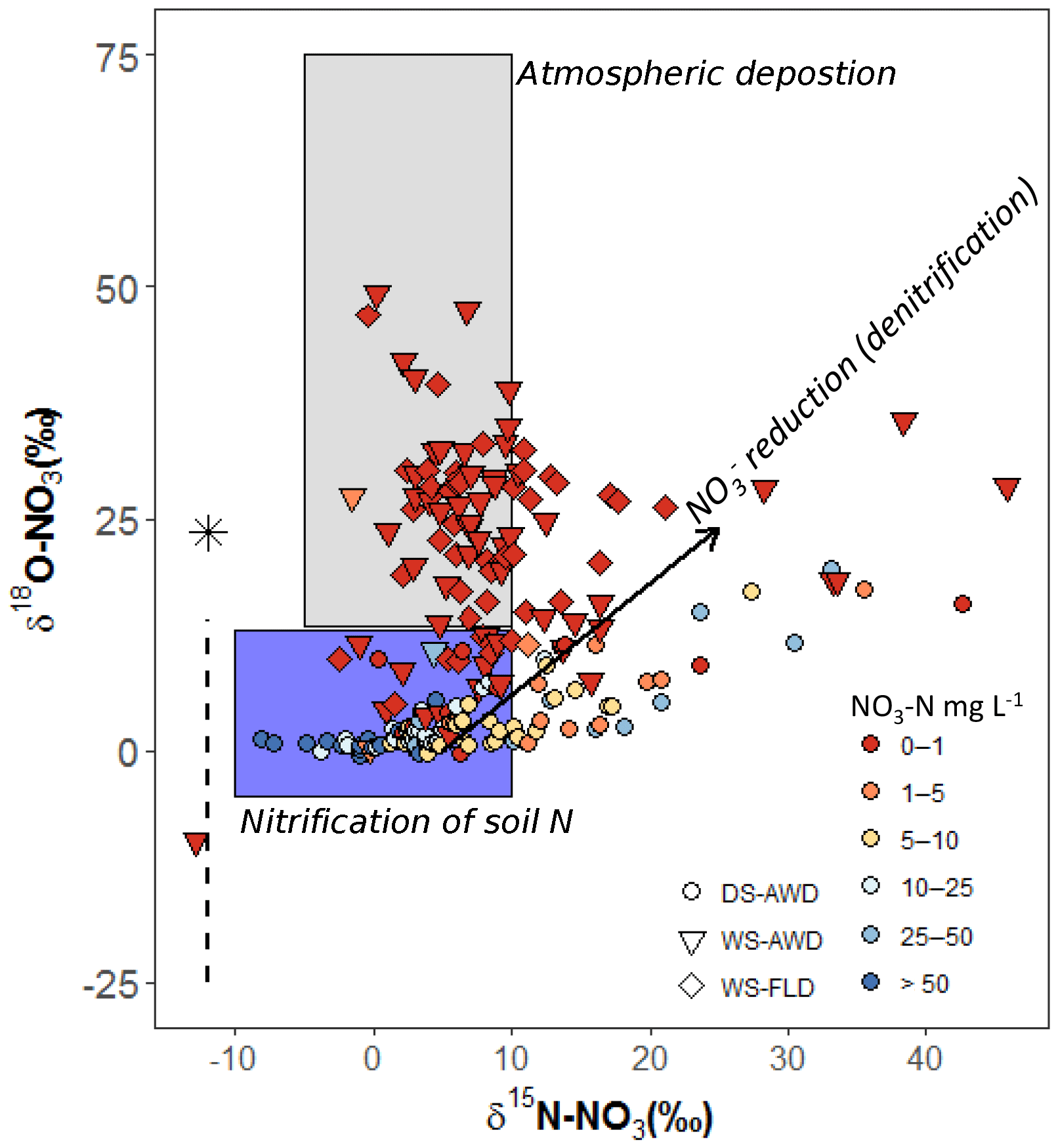
Figure 7Relationship of δ18O- to δ15N- in pore water samples of the three water management treatments (WS-FLD: water-seeding + conventional flooding; WS-AWD: water-seeding + alternate wetting and drying; DS-AWD: direct dry seeding + alternate wetting and drying). After Kendall and McDonnell (2012). The black arrow represents the trajectory of reduction effects. The black asterisk signifies the δ18O value atmospheric O2 (25.3 ‰) while the dashed black line indicates the range of δ18O in soil water. δ18O−H2O was not directly measured in our study. We assumed a value of −8.3 ‰ taken from an uncontained aquifer in the region by Rapti-Caputo and Martinelli (2009). The symbol colors indicate the concentration of in each sample (mg L−1).
4.3 Inferring the extent of N2O reduction
It has been suggested that the slope of SP/δ18O, SP/ δ15N and δ18O δ∕15N or their isotope effects can be used to estimate the extent of N2O reduction (Jinuntuya-Nortman et al., 2008; Well and Flessa, 2009; Lewicka-Szczebak et al., 2017; Ostrom et al., 2007). However, many studies deriving these relationships have taken place under controlled conditions when N2O supply was often limited. Therefore, fractionation following closed-system dynamics would result in larger fractionation effects on the residual substrate than under open-system dynamics. The positive and significant relationship between all isotopes and across all depths in the DS-AWD treatment suggests an influence of reduction at all depths. In contrast, in the WS treatments we observed no relationship between SP and δ18O within N2Oemitted (Fig. S7) and only a weak relationship between SP and δ15N at 25 cm in the WS-AWD and even a negative relationship between SP and δ15N in the WS-FLD N2Oemitted (Fig. S8). The range of observed δ18O/ δ15N slopes (0.21 to 0.90; Fig. S5) was substantially lower than those observed in many N2O reduction studies (1.94 to 2.6; Jinuntuya-Nortman et al., 2008; Ostrom et al., 2007; Well and Flessa, 2009; Lewicka-Szczebak et al., 2017) but closer to the 0.45 slope observed by Yano et al. (2014) in an in situ rice field study. When a significant relationship was observed, overall or N2Oporeair SP∕δ15N slopes ranged from 0.49 to 0.83 (Fig. 4b). These slopes are either close to those of other field studies (0.48 to 0.52; Yano et al., 2014; Wolf et al., 2015) or intermediary between field studies and controlled N2O reduction studies (0.59 to 1.01; Well and Flessa, 2009; Lewicka-Szczebak et al., 2017). From controlled N2O reduction studies, an SP∕δ18O slope between 0.2 to 0.4 has been observed (Jinuntuya-Nortman et al., 2008; Well and Flessa, 2009); thus, in this case the N2Oporeair slopes observed in our study were substantially higher (Figs. 4a and S7). The lower overall SP and δ18O slope in the WS treatments was due to the inclusion of the N2Oemitted values, which individually showed no relationship in these treatments.
A deviation in slopes compared to those observed in controlled N2O reduction studies likely points to a growing influence of open-system dynamics where substrates are continuously refreshed. It has been demonstrated that when mixing processes dominate over reduction processes, the SP∕δ18O slope rises (Lewicka-Szczebak et al., 2017). It is also plausible that high rates of oxygen exchange during denitrification served to partially mask an increase in δ18O-N2O values, resulting in the higher observed SP/δ18O slopes or lower δ18O∕δ15N slopes. To estimate the extent of oxygen exchange with denitrification precursors (NOx) we plotted by - following Snider et al. (2009). The slope of this relationship ranged from 0.7 to 2.1 (data not shown). Thus, we assume oxygen exchange was effectively 100 % across treatments during denitrification. In summary, the observed positive relationships between the isotope pairs is indicative of an influential role of N2O reduction in the DS-AWD treatment. This is less clear in the WS treatments where relationships were more erratic, suggesting a stronger influence of changing nitrification and denitrification process rates or changing δ15N of N substrates. It is likely that isotope ratios in the WS treatments were affected by near-complete denitrification to N2. Well et al. (2012) observed highly variable isotope ratios in a strongly denitrifying aquifer and concluded that N2O reduction was strongly progressed but variable. However, it should be noted that their system had abundant while ours did not. The inconsistent relationships between N2Oemitted and N2Oporeair for SP∕δ15N and SP∕δ18O in the WS treatments and the stronger enrichment observed in the DS-AWD N2Oemitted (Fig. 4) demonstrate a disconnection between subsurface N2Oemitted and N2Oporeair across treatments. Such results suggest that N2O reduction may not have had as strong of an influence on the signature of N2Oemitted as it did on N2Oporeair, particularly in the WS treatments. A decoupling between subsurface N2O concentrations and surface emissions and their isotope ratios has been observed in other studies (Van Groenigen et al., 2005; Goldberg et al., 2010a). This phenomenon is most simply explained by emitted N2O truly coming from a mix of sources and depths, while subsurface N2O is representative of a much smaller spatial zone and more likely to be dominated by one process. While difficult to practically measure, processes at shallow depths above 5 cm were also likely influential to surface emissions.
4.4 Complementary evidence from a two end-member mixing model approach
To quantitatively estimate the extent of N2O reduction (gross rN2O), N2O production and reduction rates, and the contribution of denitrification to N2O emissions, we used an open- and closed-system two end-member mixing model based on SP-N2O and δ18O-N2O relationships. As described in Sect. 2.7, we tested our models under two scenarios; in scenario 1 (sc1) N2O is produced and reduced by denitrifiers before mixing with N2O derived from nitrification; in scenario 2 (sc2) N2O is produced from both processes, mixed and then reduced (Fig. 1). While we could estimate gross rN2O and the fraction of denitrification from both scenarios, sc2 yielded mostly implausible solutions for the contribution of denitrification to N2O in open systems (Fig. S3 and Table S2). We thus conclude that the assumptions underlying this scenario in open systems were not valid in our system. In a closed system N2O is progressively consumed and not replenished, resulting in a stronger isotope effect and faster enrichment of the remaining N2O; thus, a smaller degree of N2O reduction is needed to achieve an equivalent enrichment as in open systems. Our results for open and closed systems align well with this theory on N2O fractionation. However, we feel strongly that with in situ measurements in a heterogeneous soil environment, a combination of closed- and open-system dynamics likely exits; therefore, the following interpretation of our data is based on an average of open- and closed-system values. Given the lower moisture and evidence of extensive nitrification occurring in the DS-AWD treatment, we expected a higher contribution of nitrification/fungal denitrification in this treatment, coming from an increase in nitrification. However, this was not the case and denitrification/nitrifier-denitrification contributions tended to be higher in the DS-AWD treatment relative to WS treatments (Figs. 5a, 6). Treatment differences were significant in the surface fluxes; however, there was a significant interaction with sampling day. There was no treatment effect on denitrification contribution in the subsurface (Table 5). The equivalent or higher contributions of nitrification/fungal denitrification in the WS treatments (Fig. 6) are most easily explained by higher fungal denitrification; in their laboratory experiments, Lewicka-Szczebak et al. (2017) also observed relatively high fungal denitrification contributions under very wet conditions. Larger contributions from fungal denitrification would also help explain the less clear reduction trends as fungal denitrifiers are thought to largely produce N2O as an end-product rather than N2. It should be noted that due to low surface fluxes or N2Oporeair, we had fewer data points in the WS treatments. Previous studies have attributed significant amounts of N2O emissions in paddy systems to nitrification in periods of low soil moisture (Lagomarsino et al., 2016; Verhoeven et al., 2018). Yet such studies were not able to quantitatively source partition emissions. Given our results here, it is possible that N2O produced either via nitrifier denitrification or coupled nitrification–denitrification has been previously underestimated.
The modeled gross rN2O fractions indicate high levels of N2O reduction for all treatments and depths, (rN2O: 0.06 to 0.19) even in the DS-AWD where soil moisture was frequently below 60 % at 5 cm (Fig. 2). These results are at first surprising, but there is still much we do not know about subsurface N2O production and consumption. Direct measurements of N2O reduction at depth are few. Using membrane inlet mass spectrometry, Zhou et al. (2017) detected higher N2O reduction to N2 in paddy soil water at 20 cm versus 60 or 80 cm and could relate this to higher DOC concentrations at 20 cm. Other studies suggest high subsurface N2O reduction based on the inference of declining N2O concentration accompanied by isotope enrichment moving up a soil profile (Goldberg et al., 2008; Clough et al., 1998; Van Groenigen et al., 2005). We are also methodologically limited by our inability to measure N2O isotopes at near or complete N2O reduction because there is too little remaining N2O to measure. We assume this was more often the case in the WS treatments; therefore, we postulate that the signature of N2O reduction was stronger in the DS-AWD largely because there was more N2O left to measure. In their experiments to validate the mixing model we used, Lewicka-Szczebak et al. (2017) found that the model routinely underestimated gross rN2O rates relative to measured rates in an oxic mineral soil but performed better under anoxic conditions and in an organic soil. Therefore, an underestimation of rN2O rates, particularly in the DS-AWD treatments, remains possible. However, considering the strong indication of N2O reduction from other isotope relationships (i.e., SP and δ15N and δ15N and δ18O), we believe that subsurface N2O reduction rates were simply high in our system, regardless of water management.
Table 6Spearman correlations between modeled rN2O-gross, fracDEN-gross and DenContribution with soil environmental variables and inorganic N substrates and δ15N-N2O. Results are for the mean of open- and closed-system dynamics. Subsurface correlations were performed on data aggregated across 5 and 12.5 cm depths. Significance indicated by < 0.0001, < 0.001, < 0.01, * < 0.05.
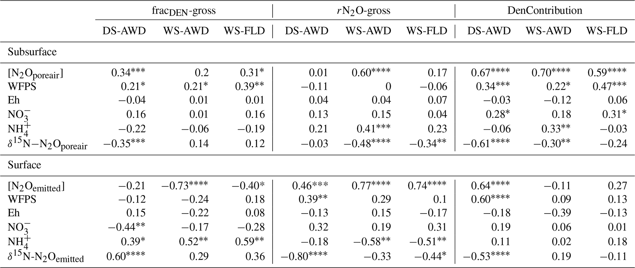
In the subsurface, the contribution of denitrification/nitrifier denitrification to N2O concentrations was positively correlated to N2Oporeair concentrations and WFPS in all treatments, indicating an increasing contribution of denitrification/nitrifier denitrification at times of higher N2O production in conjunction with rising soil moisture (Table 6). In the two AWD treatments, the contribution of denitrification/nitrifier denitrification negatively correlated to δ15N signature of N2Oporeair and N2Oemitted (DS-AWD only). Many studies have demonstrated that high subsurface N2O production is correlated to depleted δ15N-N2O (Goldberg et al., 2008, 2010b; Van Groenigen et al., 2005). These results further support the conclusion that high N2Oporeair and N2Oemitted were produced from denitrification/nitrifier denitrification associated with more depleted δ15N-N2O. Higher gross rN2O (less N2O reduction) was associated with higher N2Oemitted in all treatments and higher N2Oporeair (WS-AWD only), demonstrating that higher N2O resulted not only from increased denitrification/nitrifier denitrification but also from a decrease in N2O reduction. Interestingly, higher rN2O in N2Oemitted of the DS-AWD was also associated with higher WFPS. Such a result can only be explained by a dependency of reduction on N2O production. Overall, there was a negative relationship between rN2O and δ15N-N2O, yet the relationship was not consistently strong or significant between treatments. A negative relationship supports an isotope enrichment effect with greater N2O reduction. Considering the above, it appears that maximum N2O production and emissions occurred during periods of increased contribution from denitrification/nitrifier denitrification, which were accompanied by small declines in N2O reduction. These relationships were most robust in the DS-AWD treatment. Correlations within the N2Oemitted dataset were undoubtedly affected by lower data availability, particularly in the WS treatments, and should be taken with caution. Despite the high estimates of N2O reduction for all treatments, we still observed relevant contributions from nitrification/fungal denitrification on many dates (Fig. 6). Nevertheless, the highest fluxes in the DS-AWD aligned with higher contributions from denitrification/nitrifier denitrification, while the highest fluxes in the WS treatment had nitrification/fungal denitrification contributions of ca. 50 %. In the WS treatments we again postulate that fungal denitrification rates increased because conditions were not ideal for high nitrification. Studies have shown that fungal denitrification and co-denitrification can play a significant role in soil N2 and N2O emissions from soil (Long et al., 2013; Laughlin and Stevens, 2002).
From our modeling results we could estimate N2 production or emissions based on our calculated N2O reduction rates (Fig. S13). Due to poor data availability and high variability, we could neither confidently estimate N2 production at 25 cm nor surface N2 emissions on many dates of the WS treatments, but we have more confidence in the estimates obtained for the DS-AWD treatment. Mean daily N2 emissions found in our study were 236±53 (n=43), 194±37 (n=41) and 197±35 (n=31) g N ha−1 d−1 in the DS-AWD, WS-AWD and WS-FLD, respectively. To our knowledge only one other study by Yano et al. (2014) has conducted similar calculations to estimate N2 emissions in rice systems from isotope ratios. The authors also found high rates of N2O reduction, around 80 % to 85 %, corresponding to an rN2O of 0.15 to 0.20 and N2 emissions between 0.1 to 422 µg N m2 h−1 (or 0.024 to 101.4 g ha−1 d−1). Therefore, the estimated extent of N2O reduction was quite similar to our surface-emitted reduction rates, with somewhat lower N2 emissions corresponding to somewhat lower N2O emissions. Using labeled 15N urea, Lindau et al. (1990) measured N2 emissions of 254 g ha−1 d−1, while Dong et al. (2012) observed similar rates of 194 g N2-N ha−1 d−1 for an AWD treatment. Considering that these results only account for N2 derived from fertilizer, the modeled mean daily N2 emissions found in our study are plausible. Differences between the treatment means were not significant for N2Oporeair or N2Oemitted (p=0.431 and p=0.858) and thus do not indicate a higher potential for N2 losses in the WS treatments. We must reject our hypothesis that higher in the WS-AWD relative to the WS-FLD would drive higher denitrification and N2 losses because we observed no differences in final modeled N2 production and concentrations were essentially zero for both WS treatments. Our results show there is promise for estimating N2 emissions from N2O isotope ratios using simple models, but the precision of these estimates remains constrained by the limitations discussed below.
All modeling attempts to date rely on isotope signatures and effects determined in laboratory studies, and thus changes in these values in response to environmental or microbial population dynamics in the field remain a large question. As this was an in situ field experiment, conditions were not constant across treatments or throughout the sampling time frame, yet it has been shown that isotope effects, particularly for N2O reduction, change with shifts in environmental conditions such as increasing water-filled pore space (Jinuntuya-Northman et al., 2008). Therefore, the use of fixed isotope effects in our model is a simplification. Future modeling efforts may be improved by the incorporation of variable isotope effects based on soil moisture or O2 for example. Careful, controlled experiments across a range of soils with different management histories are necessary to determine if consistent variation in isotope effects in relation to specific environmental parameters can be determined or if such parameters are site specific. The microbial δ18O signature for denitrification used in our model was calculated relative to δ18O-H2O. We therefore assumed complete exchange between N2O substrates, intermediaries and water during denitrification. We based this on previous work showing that O exchange is high and that the isotope effect between water and N2O is relatively stable (Lewicka-Szczebak et al., 2016, 2017; Snider et al., 2013; Kool et al., 2007). In reality, results over time and between treatments may have been affected by varying degrees of 18O exchange between N2O, intermediaries and water and by variation in δ18O−H2O values. We recommend that future studies measure the δ18O-H2O to better constrain results. Modeling results would also be more robust if complete δ15N -N2O, - and - across treatments and times were available, allowing for complementary modeling of SP × 15N( or N2O∕NH4). As an exploration of model sensitivity to the isotope signature used, we evaluated results across a range of nit and den values (Fig. S14) before selecting those used in Lewicka-Szczebak et al. (2017). More elaborate modeling efforts could employ iterative simulation techniques where a range of literature values for N2O signatures and isotope effects are used and drawn to help highlight model sensitivity to specific isotope values and improve its accuracy. Lastly, more work needs to be done to validate results such as those generated here which rely on laboratory derived values, with complementary measurements of microbial community dynamics, such as that by Snider et al. (2015).
The relatively dry conditions in the DS-AWD treatment and application of urea fertilizer led to extensive nitrification, subsequent denitrification and denitrification-derived N2O emissions. Even with evidence of nitrification and relatively aerobic conditions in the DS-AWD treatment, both graphical and two end-member mixing model results indicated significant N2O reduction in all treatments, graphically most convincingly in the DS-AWD treatment. Treatment differences may also reflect paddy history as this was the fifth year of alternative water management at the site. Yields were also lower in the DS-AWD, which likely lowered N demand and increased soil N concentrations in this treatment. Differences between depths were often more evident in N2Oporeair, , and DOC concentrations than in N2O isotope signatures at the various depths, particularly for the WS treatments. In the DS-AWD treatment, isotope signatures of δ18O-N2O and SP values demonstrated notably lower values at 5 cm relative to other depths, mostly likely indicating higher N2O production and less reduction in the upper layer. Overall, the highest N2O production and emissions were associated with an increasing contribution from denitrification/nitrifier denitrification accompanied by decreases in N2O reduction in the AWD treatments. Our isotope data suggest that contributions from fungal denitrification to N2O emissions may have increased in the WS-FLD treatment. The role of fungal denitrification in paddy rice systems should be further investigated with the use of fungal inhibitors. Surface-emitted N2O reduction rates were similar for all treatments; therefore, our hypothesis of a greater potential for gaseous N2 losses in the WS-AWD is refuted. Despite the difficulty in obtaining a full dataset for all treatments and the inherent spatiotemporal variability in the original measured fluxes, we came to good agreement with the magnitude of N2 emissions reported from previous 15N labeled fertilizer studies. Thus, natural abundance isotope methods do show promise for estimating N2 emissions and closing N budgets, even without the δ15N of N substrates. Model results would likely improve with controlled incubations to determine site-specific isotope effects and whether these effects change in a consistent manner with specific environmental conditions. In saturated or partly saturated systems, future studies should probe the disconnection between subsurface and emitted N2O isotopes by employing methods that allow for larger subsurface spatial integration along vertical and horizontal planes. It appears that to effectively manage N losses in alternative water management paddy systems, the inhibition of nitrification is necessary, particularly very early in the growing season when N availability exceeds crop N demand.
The dataset supporting these results is available on the open-access platform Zenodo (https://doi.org/10.5281/zenodo.1251895; Verhoeven, 2018).
The supplement related to this article is available online at: https://doi.org/10.5194/bg-16-383-2019-supplement.
The field work, initial analysis, modeling and primary manuscript preparation was carried out by EV. Isotope ratio analysis and technical and analytical support was provided by MB. Open system model conception was devised by CD. Closed system model conception and support was provided by DLS. CD advised extensively on data and model analysis. SS, CD and JS were responsible for the original project conception. All authors contributed manuscript preparation and revisions.
The authors declare that they have no conflict of interest.
This work was financially supported by the Swiss National Science Foundation
(40FA40_154246) through the Joint Programming Initiative on
Agriculture, Food Security and Climate Change (FACCE-JPI). This work would
not have been possible without the support and assistance of the staff at
Ente Nazionale Risi in Castello D'Agogna, Italy, in particular Marco Romani,
Elenora Miniotti and Daniele Tenni.
Edited by: Andreas Richter
Reviewed by: Nathaniel Ostrom and one anonymous referee
Agenzia Regionale per la Protezione dell'Ambiente-Lomardia: Regional Agency for the Protection of the Environment, Lombardy, Pavia, Castello D'Agogna, available at: http://www.arpalombardia.it/siti/arpalombardia/meteo/richiesta-dati-misurati/Pagine/RichiestaDatiMisurati.aspx, last access: 15 January 2019.
Arth, I. and Frenzel, P.: Nitrification and denitrification in the rhizosphere of rice: the detection of processes by a new multi-channel electrode, Biol. Fert. Soils, 31, 427–435, https://doi.org/10.1007/s003749900190, 2000.
Aulakh, M. S., Khera, T. S., Doran, J. W., and Bronson, K. F.: Denitrification, N2O and CO2 fluxes in rice-wheat cropping system as affected by crop residues, fertilizer N and legume green manure, Biol. Fert. Soils, 34, 375–389, https://doi.org/10.1007/s003740100420, 2001.
Baggs, E. M.: A review of stable isotope techniques for N2O source partitioning in soils: recent progress, remaining challenges and future considerations, Rapid Commun. Mass Sp., 22, 1664–1672, https://doi.org/10.1002/rcm.3456, 2008.
Bremner, J., Blackmer, A., and Waring, S.: Formation of nitrous oxide and dinitrogen by chemical decomposition of hydroxylamine in soils, Soil Biol. Biochem., 12, 263–269, 1980.
Butterbach-Bahl, K., Baggs, E. M., Dannenmann, M., Kiese, R., and Zechmeister-Boltenstern, S.: Nitrous oxide emissions from soils: how well do we understand the processes and their controls?, Philos. T. R. Soc. B, 368, 13 pp., https://doi.org/10.1098/rstb.2013.0122, 2013.
Cai, Z., Xing, G., Yan, X., Xu, H., Tsuruta, H., Yagi, K., and Minami, K.: Methane and nitrous oxide emissions from rice paddy fields as affected by nitrogen fertilisers and water management, Plant Soil, 196, 7–14, 1997.
Casciotti, K. L., Sigman, D. M., Hastings, M. G., Bohlke, J. K., and Hilkert, A.: Measurement of the oxygen isotopic composition of nitrate in seawater and freshwater using the denitrifier method, Anal. Chem., 74, 4905–4912, https://doi.org/10.1021/ac020113w, 2002.
Cassman, K. G., Peng, S., Olk, D. C., Ladha, J. K., Reichardt, W., Dobermann, A., and Singh, U.: Opportunities for increased nitrogen-use efficiency from improved resource management in irrigated rice systems, Field Crop. Res., 56, 7–39, https://doi.org/10.1016/S0378-4290(97)00140-8, 1998.
Clough, T., Jarvis, S., Dixon, E., Stevens, R., Laughlin, R., and Hatch, D.: Carbon induced subsoil denitrification of 15N-labelled nitrate in 1 m deep soil columns, Soil Biol. Biochem., 31, 31–41, 1998.
Decock, C. and Six, J.: How reliable is the intramolecular distribution of N-15 in N2O to source partition N2O emitted from soil?, Soil Biol. Biochem., 65, 114–127, https://doi.org/10.1016/j.soilbio.2013.05.012, 2013a.
Decock, C. and Six, J.: On the potential of delta O-18 and delta N-15 to assess N2O reduction to N-2 in soil, Eur. J. Soil Sci., 64, 610–620, https://doi.org/10.1111/ejss.12068, 2013b.
Dedatta, S. K., Buresh, R. J., Samson, M. I., Obcemea, W. N., and Real, J. G.: Direct Measurement of Ammonia and Denitrification Fluxes From Urea Applied to Rice, Soil Sci. Soc. Am. J., 55, 543–548, 1991.
Denk, T. R., Mohn, J., Decock, C., Lewicka-Szczebak, D., Harris, E., Butterbach-Bahl, K., Kiese, R., and Wolf, B.: The nitrogen cycle: A review of isotope effects and isotope modeling approaches, Soil Biol. Biochem., 105, 121–137, 2017.
Devkota, K. P., Manschadi, A., Lamers, J. P. A., Devkota, M., and Vlek, P. L. G.: Mineral nitrogen dynamics in irrigated rice-wheat system under different irrigation and establishment methods and residue levels in arid drylands of Central Asia, Eur. J. Agron., 47, 65–76, https://doi.org/10.1016/j.eja.2013.01.009, 2013.
Doane, T. A. and Horwáth, W. R.: Spectrophotometric determination of nitrate with a single reagent, Anal. Lett., 36, 2713–2722, 2003.
Dong, N. M., Brandt, K. K., Sørensen, J., Hung, N. N., Van Hach, C., Tan, P. S., and Dalsgaard, T.: Effects of alternating wetting and drying versus continuous flooding on fertilizer nitrogen fate in rice fields in the Mekong Delta, Vietnam, Soil Biol. Biochem., 47, 166–174, 2012.
Firestone, M. and Davidson, E.: Microbiological basis of NO and N2O production and consumption in soil, in: Exchange of trace gases between terrestrial ecosystems and the atmosphere, edited by: Andreae, M. O. and Schimel, D. S., John Wiley & Sons Ltd., USA, 7–21, 1989.
Frame, C. H. and Casciotti, K. L.: Biogeochemical controls and isotopic signatures of nitrous oxide production by a marine ammonia-oxidizing bacterium, Biogeosciences, 7, 2695–2709, https://doi.org/10.5194/bg-7-2695-2010, 2010.
Fry, B.: Stable isotope ecology, Springer, 2007.
Goldberg, S. D., Knorr, K.-H., and Gebauer, G.: N2O concentration and isotope signature along profiles provide deeper insight into the fate of N2O in soils, Isotopes in environmental and health studies, 44, 377–391, 2008.
Goldberg, S. D., Knorr, K.-H., Blodau, C., Lischeid, G., and Gebauer, G.: Impact of altering the water table height of an acidic fen on N2O and NO fluxes and soil concentrations, Glob. Change Biol., 16, 220–233, https://doi.org/10.1111/j.1365-2486.2009.02015.x, 2010a.
Goldberg, S. D., KNORR, K. H., Blodau, C., Lischeid, G., and Gebauer, G.: Impact of altering the water table height of an acidic fen on N2O and NO fluxes and soil concentrations, Glob. Change Biol., 16, 220–233, 2010b.
Heil, J., Wolf, B., Brüggemann, N., Emmenegger, L., Tuzson, B., Vereecken, H., and Mohn, J.: Site-specific 15N isotopic signatures of abiotically produced N2O, Geochim. Cosmochim. Ac., 139, 72–82, 2014.
Heil, J., Liu, S., Vereecken, H., and Brüggemann, N.: Abiotic nitrous oxide production from hydroxylamine in soils and their dependence on soil properties, Soil Biol. Biochem., 84, 107–115, 2015.
Hu, H.-W., Chen, D., and He, J.-Z.: Microbial regulation of terrestrial nitrous oxide formation: understanding the biological pathways for prediction of emission rates, FEMS Microbiol. Rev., 39, 729–749, 2015.
Hutchinson, G. and Mosier, A.: Improved soil cover method for field measurement of nitrous oxide fluxes, Soil Sci. Soc. Am. J., 45, 311–316, 1981.
IPCC: IPCC Fourth Assessment Report: Climate Change 2007: Synthesis Report, https://www.ipcc.ch/report/ar4/syr/ (last access: 15 January 2019), 2007.
Jinuntuya-Nortman, M., Sutka, R. L., Ostrom, P. H., Gandhi, H., and Ostrom, N. E.: Isotopologue fractionation during microbial reduction of N2O within soil mesocosms as a function of water-filled pore space, Soil Biol. Biochem., 40, 2273–2280, https://doi.org/10.1016/j.soilbio.2008.05.016, 2008.
Kendall, C.: Tracing Nitrogen Sources and Cycling in Catchments, in: Isotope tracers in catchment hydrology, edited by: Kendall, C. and McDonnell J. J., Elsevier, the Netherlands, 519–576, 1998.
Koba, K., Osaka, K., Tobari, Y., Toyoda, S., Ohte, N., Katsuyama, M., Suzuki, N., Itoh, M., Yamagishi, H., and Kawasaki, M.: Biogeochemistry of nitrous oxide in groundwater in a forested ecosystem elucidated by nitrous oxide isotopomer measurements, Geochim. Cosmochim. Ac., 73, 3115–3133, 2009.
Koehler, B., Corre, M. D., Steger, K., Well, R., Zehe, E., Sueta, J. P., and Veldkamp, E.: An in-depth look into a tropical lowland forest soil: nitrogen-addition effects on the contents of N2O, CO2 and CH4 and N2O isotopic signatures down to 2 m depth, Biogeochemistry, 111, 695–713, 2012.
Kool, D. M., Wrage, N., Oenema, O., Dolfing, J., and Van Groenigen, J. W.: Oxygen exchange between (de) nitrification intermediates and H2O and its implications for source determination of and N2O: a review, Rapid Commun. Mass Sp., 21, 3569–3578, https://doi.org/10.1002/rcm.3249, 2007.
Kool, D. M., Wrage, N., Oenema, O., Harris, D., and Van Groenigen, J. W.: The O-18 signature of biogenic nitrous oxide is determined by O exchange with water, Rapid Commun. Mass Sp., 23, 104–108, https://doi.org/10.1002/rcm.3859, 2009.
Kool, D. M., Wrage, N., Zechmeister-Boltenstern, S., Pfeffer, M., Brus, D., Oenema, O., and Van Groenigen, J. W.: Nitrifier denitrification can be a source of N2O from soil: a revised approach to the dual-isotope labelling method, Eur. J. Soil Sci., 61, 759–772, https://doi.org/10.1111/j.1365-2389.2010.01270.x, 2010.
Kool, D. M., Dolfing, J., Wrage, N., and Van Groenigen, J. W.: Nitrifier denitrification as a distinct and significant source of nitrous oxide from soil, Soil Biol. Biochem., 43, 174–178, https://doi.org/10.1016/j.soilbio.2010.09.030, 2011.
Lachouani, P., Frank, A. H., and Wanek, W.: A suite of sensitive chemical methods to determine the δ15N of ammonium, nitrate and total dissolved N in soil extracts, Rapid Commun. Mass Sp., 24, 3615–3623, 2010.
Lagomarsino, A., Agnelli, A. E., Linquist, B., Adviento-Borbe, M. A., Agnelli, A., Gavina, G., Ravaglia, S., and Ferrara, R. M.: Alternate wetting and drying of rice reduced CH4 emissions but triggered N2O peaks in a clayey soil of central Italy, Pedosphere, 26, 533–548, 2016.
Laughlin, R. J. and Stevens, R. J.: Evidence for fungal dominance of denitrification and codenitrification in a grassland soil, Soil Sci. Soc. Am. J., 66, 1540–1548, 2002.
Lewicka-Szczebak, D., Well, R., Koester, J. R., Fuss, R., Senbayram, M., Dittert, K., and Flessa, H.: Experimental determinations of isotopic fractionation factors associated with N2O production and reduction during denitrification in soils, Geochim. Cosmochim. Ac., 134, 55–73, https://doi.org/10.1016/j.gca.2014.03.010, 2014.
Lewicka-Szczebak, D., Dyckmans, J., Kaiser, J., Marca, A., Augustin, J., and Well, R.: Oxygen isotope fractionation during N2O production by soil denitrification, Biogeosciences, 13, 1129–1144, https://doi.org/10.5194/bg-13-1129-2016, 2016.
Lewicka-Szczebak, D., Augustin, J., Giesemann, A., and Well, R.: Quantifying N2O reduction to N2 based on N2O isotopocules – validation with independent methods (helium incubation and 15N gas flux method), Biogeosciences, 14, 711–732, https://doi.org/10.5194/bg-14-711-2017, 2017.
Haynes, W. M. and Lide, D. R. (Eds.): CRC handbook of chemistry and physics, 92nd Edn., CRC press, 5–150, 2011/2012.
Lindau, C. W., Delaune, R. D., Patrick, W. H., and Bollich, P. K.: Fertilizer Effects On Dinitrogen, Nitrous-Oxide, and Methane Emissions From Lowland Rice, Soil Sci. Soc. Am. J., 54, 1789–1794, 1990.
Long, A., Heitman, J., Tobias, C., Philips, R., and Song, B.: Co-occurring anammox, denitrification, and codenitrification in agricultural soils, Appl. Environ. Microbiol., 79, 168–176, 2013.
Maeda, K., Spor, A., Edel-Hermann, V., Heraud, C., Breuil, M.-C., Bizouard, F., Toyoda, S., Yoshida, N., Steinberg, C., and Philippot, L.: N2O production, a widespread trait in fungi, Sci. Rep., 5, 9697, https://doi.org/10.1038/srep09697, 2015.
Mariotti, A., Germon, J. C., Hubert, P., Kaiser, P., Letolle, R., Tardieux, A., and Tardieux, P.: Experimental determination of nitrogen kinetic isotope fractionation: Some principles; illustration for the denitrification and nitrification processes, Plant Soil, 62, 413–430, https://doi.org/10.1007/bf02374138, 1981.
McIlvin, M. R. and Casciotti, K. L.: Technical updates to the bacterial method for nitrate isotopic analyses, Anal. Chem., 83, 1850–1856, 2011.
Miniotti, E. F., Romani, M., Said-Pullicino, D., Facchi, A., Bertora, C., Peyron, M., Sacco, D., Bischetti, G. B., Lerda, C., and Tenni, D.: Agro-environmental sustainability of different water management practices in temperate rice agro-ecosystems, Agr. Ecosys. Envir., 222, 235–248, 2016.
Mohn, J., Wolf, B., Toyoda, S., Lin, C. T., Liang, M. C., Brüggemann, N., Wissel, H., Steiker, A. E., Dyckmans, J., Szwec, L., and Ostrom, N. E.: Interlaboratory assessment of nitrous oxide isotopomer analysis by isotope ratio mass spectrometry and laser spectroscopy: current status and perspectives, Rapid Commun. Mass Sp., 28, 1995–2007, 2014.
Mosier, A., Kroeze, C., Nevison, C., Oenema, O., Seitzinger, S., and van Cleemput, O.: Closing the global N2O budget: nitrous oxide emissions through the agricultural nitrogen cycle, Nutr. Cycl. Agroecosys., 52, 225–248, 1998.
Ostrom, N. E. and Ostrom, P. H.: The Isotopomers of Nitrous Oxide: Analytical Considerations and Application to Resolution of Microbial Production Pathways, Handbook of Environmental Isotope Geochemistry, edited by: Baskaran, M., Vol. 1 and 2, 453–476, 2011.
Ostrom, N. E., Pitt, A., Sutka, R., Ostrom, P. H., Grandy, A. S., Huizinga, K. M., and Robertson, G. P.: Isotopologue effects during N2O reduction in soils and in pure cultures of denitrifiers, J. Geophys. Res.-Biogeo., 112, 1–12, 2007.
Peyron, M., Bertora, C., Pelissetti, S., Said-Pullicino, D., Celi, L., Miniotti, E., Romani, M., and Sacco, D.: Greenhouse gas emissions as affected by different water management practices in temperate rice paddies, Agr. Ecosyst. Environ., 232, 17–28, 2016.
Rapti-Caputo, D. and Martinelli, G.: The geochemical and isotopic composition of aquifer systems in the deltaic region of the Po River plain (northern Italy), Hydrogeol. J., 17, 467–480, 2009.
Ratering, S. and Schnell, S.: Localization of iron-reducing activity in paddy soilby profile studies, Biogeochemistry, 48, 341–365, 2000.
Ravishankara, A. R., Daniel, J. S., and Portmann, R. W.: Nitrous Oxide (N2O): The Dominant Ozone-Depleting Substance Emitted in the 21st Century, Science, 326, 123–125, https://doi.org/10.1126/science.1176985, 2009.
Röckmann, T., Kaiser, J., Brenninkmeijer, C. A., and Brand, W. A.: Gas chromatography/isotope-ratio mass spectrometry method for high-precision position-dependent 15N and 18O measurements of atmospheric nitrous oxide, Rapid Commun. Mass Sp., 17, 1897–1908, 2003.
Rohe, L., Anderson, T. H., Braker, G., Flessa, H., Giesemann, A., Lewicka-Szczebak, D., Wrage-Mönnig, N., and Well, R.: Dual isotope and isotopomer signatures of nitrous oxide from fungal denitrification – a pure culture study, Rapid Commun. Mass Sp., 28, 1893–1903, 2014.
Said-Pullicino, D., Miniotti, E. F., Sodano, M., Bertora, C., Lerda, C., Chiaradia, E. A., Romani, M., Cesari de Maria, S., Sacco, D., and Celi, L.: Linking dissolved organic carbon cycling to organic carbon fluxes in rice paddies under different water management practices, Plant Soil, 401, 273–290, https://doi.org/10.1007/s11104-015-2751-7, 2016.
Schreiber, F., Wunderlin, P., Udert, K. M., and Wells, G. F.: Nitric oxide and nitrous oxide turnover in natural and engineered microbial communities: biological pathways, chemical reactions, and novel technologies, Front. Microbiol., 372, 1–24, 2012.
Seo, D. C. and DeLaune, R.: Fungal and bacterial mediated denitrification in wetlands: influence of sediment redox condition, Water Res., 44, 2441–2450, 2010.
Sigman, D. M., Casciotti, K. L., Andreani, M., Barford, C., Galanter, M., and Bohlke, J. K.: A bacterial method for the nitrogen isotopic analysis of nitrate in seawater and freshwater, Anal. Chem., 73, 4145–4153, https://doi.org/10.1021/ac010088e, 2001.
Smith, P., Martino, D., Cai, Z., Gwary, D., Janzen, H., Kumar, P., McCarl, B., Ogle, S., O'Mara, F., Rice, C., Scholes, B., Sirotenko, O., Howden, M., McAllister, T., Pan, G., Romanenkov, V., Schneider, U., Towprayoon, S., Wattenbach, M., and Smith, J.: Greenhouse gas mitigation in agriculture, Philos. T. R. Soc. B, 363, 789–813, https://doi.org/10.1098/rstb.2007.2184, 2008.
Snider, D. M., Schiff, S. L., and Spoelstra, J.: 15N∕14N and 18O∕16O stable isotope ratios of nitrous oxide produced during denitrification in temperate forest soils, Geochim. Cosmochim. Ac., 73, 877–888, https://doi.org/10.1016/j.gca.2008.11.004, 2009.
Snider, D. M., Venkiteswaran, J. J., Schiff, S. L., and Spoelstra, J.: Deciphering the oxygen isotope composition of nitrous oxide produced by nitrification, Glob. Change Biol., 18, 356–370, 2012.
Snider, D. M., Venkiteswaran, J. J., Schiff, S. L., and Spoelstra, J.: A new mechanistic model of δ18ON2O formation by denitrification, Geochim. Cosmochim. Ac., 112, 102–115, 2013.
Stanton, C. L., Reinhard, C. T., Kasting, J. F., Ostrom, N. E., Haslun, J. A., Lyons, T. W., and Glass, J. B.: Nitrous oxide from chemodenitrification: A possible missing link in the Proterozoic greenhouse and the evolution of aerobic respiration, Geobiology, 16, 597–609, 2018.
Stephan, K. and Kavanagh, K.: Suitability of the Diffusion Method for Natural Abundance Nitrogen-15 Analysis, Soil Sci. Soc. Am. J., 73, 293–302, 2009.
Sutka, R. L., Ostrom, N., Ostrom, P., Breznak, J., Gandhi, H., Pitt, A., and Li, F.: Distinguishing nitrous oxide production from nitrification and denitrification on the basis of isotopomer abundances, Appl. Environ. Microbiol., 72, 638–644, 2006.
Sutka, R. L., Adams, G. C., Ostrom, N. E., and Ostrom, P. H.: Isotopologue fractionation during N2O production by fungal denitrification, Rapid Commun. Mass Sp., 22, 3989–3996, 2008.
Toyoda, S., Yano, M., Nishimura, S. i., Akiyama, H., Hayakawa, A., Koba, K., Sudo, S., Yagi, K., Makabe, A., and Tobari, Y.: Characterization and production and consumption processes of N2O emitted from temperate agricultural soils determined via isotopomer ratio analysis, Global Biogeochem. Cy., 25, 1–17, 2011.
USDA-NRCS: Keys to Soil Taxonomy, 11th edn., USDA-Natural Resources Conservation Service, Washington, DC, 2010.
Van Groenigen, J. W., Zwart, K. B., Harris, D., and van Kessel, C.: Vertical gradients of delta N-15 and δ(18O) in soil atmospheric N2O-temporal dynamics in a sandy soil, Rapid Commun. Mass Sp., 19, 1289–1295, https://doi.org/10.1002/rcm.1929, 2005.
Venterea, R. T., Halvorson, A. D., Kitchen, N., Liebig, M. A., Cavigelli, M. A., Grosso, S. J. D., Motavalli, P. P., Nelson, K. A., Spokas, K. A., and Singh, B. P.: Challenges and opportunities for mitigating nitrous oxide emissions from fertilized cropping systems, Front. Ecol. Environ., 10, 562–570, 2012.
Verhoeven, E.: CastelloD'Agogna_waterMgmt2015,2016_dataset (Version 1.0), Zenodo, https://doi.org/10.5281/zenodo.1251895, 2018.
Verhoeven, E. and Six, J.: Biochar does not mitigate field-scale N2O emissions in a Northern California vineyard: an assessment across two years, Agr. Ecosys. Environ., 191, 27–38. 2014
Verhoeven, E., Pereira, E., Decock, C., Garland, G., Kennedy, T., Suddick, E., Horwath, W. R., and Six, J.: N2O emissions from California farmlands: A review, Calif. Agr., 71, 148–159, https://doi.org/10.3733/ca.2017a0026, 2017.
Verhoeven, E., Decock, C., Barthel, M., Bertora, C., Sacco, D., Romani, M., Sleutel, S., and Six, J.: Nitrification and coupled nitrification-denitrification at shallow depths are responsible for early season N2O emissions under alternate wetting and drying management in an Italian rice paddy system, Soil Biol. Biochem., 120, 58–69, https://doi.org/10.1016/j.soilbio.2018.01.032, 2018.
Weiss, R. and Price, B.: Nitrous oxide solubility in water and seawater, Mar. Chem., 8, 347–359, 1980.
Well, R. and Flessa, H.: Isotopologue enrichment factors of N2O reduction in soils, Rapid Commun. Mass Sp., 23, 2996–3002, 2009.
Well, R., Eschenbach, W., Flessa, H., von der Heide, C., and Weymann, D.: Are dual isotope and isotopomer ratios of N2O useful indicators for N2O turnover during denitrification in nitrate-contaminated aquifers?, Geochim. Cosmochim. Ac., 90, 265–282, 2012.
Wilhelm, E., Battino, R., and Wilcock, R. J.: Low-pressure solubility of gases in liquid water, Chem. Rev., 77, 219–262, 1977.
Wolf, B., Merbold, L., Decock, C., Tuzson, B., Harris, E., Six, J., Emmenegger, L., and Mohn, J.: First on-line isotopic characterization of N2O above intensively managed grassland, Biogeosciences, 12, 2517–2531, https://doi.org/10.5194/bg-12-2517-2015, 2015.
Wrage, N., Velthof, G., Van Beusichem, M., and Oenema, O.: Role of nitrifier denitrification in the production of nitrous oxide, Soil Biol. Biochem., 33, 1723–1732, 2001.
Wu, D., Köster, J. R., Cárdenas, L. M., Brüggemann, N., Lewicka-Szczebak, D., and Bol, R.: N2O source partitioning in soils using 15N site preference values corrected for the N2O reduction effect, Rapid Commun. Mass Sp., 30, 620–626, 2016.
Xu, Y., Ge, J., Tian, S., Li, S., Nguy-Robertson, A. L., Zhan, M., and Cao, C.: Effects of water-saving irrigation practices and drought resistant rice variety on greenhouse gas emissions from a no-till paddy in the central lowlands of China, Sci. Total Environ., 505, 1043–1052, 2015.
Yano, M., Toyoda, S., Tokida, T., Hayashi, K., Hasegawa, T., Makabe, A., Koba, K., and Yoshida, N.: Isotopomer analysis of production, consumption and soil-to-atmosphere emission processes of N2O at the beginning of paddy field irrigation, Soil Biol. Biochem., 70, 66–78, https://doi.org/10.1016/j.soilbio.2013.11.026, 2014.
Yao, S.-H., Zhang, B., and Hu, F.: Soil biophysical controls over rice straw decomposition and sequestration in soil: the effects of drying intensity and frequency of drying and wetting cycles, Soil Biol. Biochem., 43, 590–599, 2011.
Zhou, W., Xia, L., and Yan, X.: Vertical distribution of denitrification end-products in paddy soils, Sci. Total Environ., 576, 462–471, 2017.
Zhou, Z., Takaya, N., Sakairi, M. A. C., and Shoun, H.: Oxygen requirement for denitrification by the fungus Fusarium oxysporum, Arch. Microbiol., 175, 19–25, 2001.
Zhu-Barker, X., Cavazos, A. R., Ostrom, N. E., Horwath, W. R., and Glass, J. B.: The importance of abiotic reactions for nitrous oxide production, Biogeochemistry, 126, 251–267, 2015.
Zou, Y., Hirono, Y., Yanai, Y., Hattori, S., Toyoda, S., and Yoshida, N.: Isotopomer analysis of nitrous oxide accumulated in soil cultivated with tea (Camellia sinensis) in Shizuoka, central Japan, Soil Biol. Biochem., 77, 276–291, 2014.