High-frequency measurements explain quantity and quality of dissolved organic carbon mobilization in a headwater catchment

Increasing dissolved organic carbon (DOC) concentrations and exports from headwater catchments impact the quality of downstream waters and pose challenges to water supply. The importance of riparian zones for DOC export from catchments in humid, temperate climates has generally been acknowledged, but the hydrological controls and biogeochemical factors that govern mobilization of DOC from riparian zones remain elusive. A high-frequency dataset (15 min resolution for over 1 year) from a headwater catchment in the Harz Mountains (Germany) was analyzed for dominant patterns in DOC concentration (C_DOC) and optical DOC quality parameters SUVA₂₅₄ and S_275−295 (spectral slope between 275 and 295 nm) on event and seasonal scales. Quality parameters and C_DOC systematically changed with increasing fractions of high-frequency quick flow (Q_hf) and antecedent hydroclimatic conditions, defined by the following metrics: aridity index (AI₆₀) of the preceding 60 d and the quotient of mean temperature (T₃₀) and mean discharge (Q₃₀) of the preceding 30 d, which we refer to as discharge-normalized temperature (DNT₃₀). Selected statistical multiple linear regression models for the complete time series (R²=0.72, 0.64 and 0.65 for C_DOC, SUVA₂₅₄ and S_275−295, resp.) captured DOC dynamics based on event (Q_hf and baseflow) and seasonal-scale predictors (AI₆₀, DNT₃₀). The relative importance of seasonal-scale predictors allowed for the separation of three hydroclimatic states (warm and dry, cold and wet, and intermediate). The specific DOC quality for each state indicates a shift in the activated source zones and highlights the importance of antecedent conditions and their impact on DOC accumulation and mobilization in the riparian zone. The warm and dry state results in high DOC concentrations during events and low concentrations between events and thus can be seen as mobilization limited, whereas the cold and wet state results in low concentration between and during events due to limited DOC accumulation in the riparian zone. The study demonstrates the considerable value of continuous high-frequency measurements of DOC quality and quantity and its (hydroclimatic) key controlling variables in quantitatively unraveling DOC mobilization in the riparian zone. These variables can be linked to DOC source activation by discharge events and the more seasonal control of DOC production in riparian soils.

1 Introduction

Dissolved organic carbon (DOC) in streams is a significant part of the global carbon cycle (Battin et al., 2009) and plays a vital role as a nutrient for aquatic ecosystems. Riverine exports of DOC from catchments can impair downstream aquatic ecology and water quality (Hruška et al., 2009) with potential implications for the treatment of drinking water from surface water reservoirs (Alarcon-Herrera et al., 1994). The pivotal role of DOC for surface water quality and ecology is not only related to the concentration (C_DOC) in the water, but also to the specific chemical composition of DOC, referred to here as DOC quality. For example, DOC quality defines the thermodynamically available energy (Stewart and Wetzel, 1981), which in turn affects the growth of microorganisms (Ågren et al., 2008). Consequently, changes in DOC quality could change the patterns of aquatic microbial metabolism resulting in altered ecosystem functioning (Berggren and del Giorgio, 2015). For managing water quality and aquatic ecology in surface waters, it is therefore not only important to understand the drivers and controls of DOC concentration, but also of the associated DOC quality. This study takes a step in this direction.

DOC concentrations in streams were found to be highly variable in time with strong controls being discharge (Zarnetske et al., 2018), climatic conditions (Winterdahl et al., 2016), or at longer timescales the prevailing biogeochemical regime (Musolff et al., 2017). DOC concentration variability is also closely linked to distinct DOC source zones in catchments and their hydrologic connectivity to the stream network (Broder et al., 2015; Birkel et al., 2017). In temperate humid climates most of the riverine DOC export is typically derived from terrestrial sources at or near the terrestrial–aquatic interface (Laudon et al., 2012; Ledesma et al., 2018; Musolff et al., 2018; Zarnetske et al., 2018). More specifically, the riparian zone is seen as a dominant source zone for DOC, defining potential DOC export loads and their temporal patterns (Ledesma et al., 2015; Musolff et al., 2018). In this zone, DOC export is strongly controlled by lateral hydrologic transport through shallow organic-rich soil layers, thus connecting different patches of differently processed DOC pools to the stream. The capacity of the riparian zone to drain and produce discharge and thus export DOC generally increases with the rise of the groundwater table during events. This causes a nonlinear increase in the lateral transmissivity of the riparian soil profile and the resulting subsurface flux to the stream, which has been called the transmissivity feedback mechanism (Bishop et al., 2004; Rodhe, 1989). However, distinct preferential flow paths in the subsurface (Hrachowitz et al., 2016) and at the surface (Frei et al., 2010) can also play a considerable role. The associated DOC export to the streams was found to be mostly transport limited (Zarnetske et al., 2018) with storm events generally generating most of the overall loads exported from catchments (Buffam et al., 2001; Hope et al., 1994). Daily precipitation and amount of discharge were found to be event-scale drivers (Bishop et al., 1990) defining magnitude and timing of DOC export. Strohmeier et al. (2013) therefore pointed at the importance of temporally resolved concentration measurements for accurate load estimates.

In addition to discharge and transport capacity, the biogeochemical regime in the riparian soils, which controls the buildup, size and quality of the exportable DOC pool, was identified as an additional important control for DOC export from catchments (Winterdahl et al., 2016). This buildup of exportable DOC pools in turn is strongly related to the hydroclimatic conditions like temperature and soil moisture content prior to an event (Birkel et al., 2017; Broder et al., 2017; Christ and David, 1996; Garcia-Pausas et al., 2008; Preston et al., 2011), which to some degree also define the potential for hydrological connectivity and transport during the event (Birkel et al., 2017; Köhler et al., 2009; Shang et al., 2018). On a seasonal scale (roughly 1–3 months) hydroclimatic variables control intra-annual variability of DOC concentration and quality (Ågren et al., 2007; Hope et al., 1994; Köhler et al., 2009) and are hence considered important drivers of seasonal DOC export dynamics (Ågren et al., 2007; Birkel et al., 2014; Köhler et al., 2009; Seibert et al., 2009). In summary, DOC concentration and quality are jointly controlled by the hydrologic conditions during events (defining the timing and magnitude of DOC export) and the antecedent hydroclimatic conditions (defining size and quality of exportable DOC pools in the soil), resulting in a highly dynamic system with processes interacting at timescales ranging from the event scale of hours to days to timescales of seasons. Characterizing and quantifying such a dynamic system requires measurements of DOC concentration and quality at a sufficient temporal resolution. Yet, most studies to date have only focused on temporally aggregated data (Köhler et al., 2008) and the seasonal to annual timescale with little or no consideration of the strong interaction with event-scale variability of DOC quantity and quality (Bishop et al., 1990; Strohmeier et al., 2013).

Recent years have seen significant advances in sensing technologies for high-frequency in situ concentration measurements (Rode et al., 2016; Strohmeier et al., 2013), facilitating the assessment of the highly dynamic DOC delivery to streams (Tunaley et al., 2016). Differences in DOC quality observed during varying runoff conditions have been used to characterize source zone activation in smaller watersheds (Hood et al., 2006; Sanderman et al., 2009). Hence, the combination of high-frequency C_DOC measurements with additional spectral and analytical methods to characterize DOC quality (Herzsprung et al., 2012; Raeke et al., 2017; Roth et al., 2013) at temporal resolutions capable of capturing the dynamics within hydrologic events provides an opportunity to significantly improve our mechanistic understanding of DOC mobilization, transport, and ultimately export from catchments (Berggren and del Giorgio, 2015; Creed et al., 2015; Köhler et al., 2009; Strohmeier et al., 2013). Broder et al. (2017) jointly evaluated DOC concentration and quality dynamics, but they were limited to hourly event data and data once every 2 weeks between events. Here we see great potential in the systematic analysis of high-frequency data for improving our understanding of the delicate interplay between hydrologic (mobilization and transport) and biogeochemical controls (buildup of exportable DOC pools) from the event to seasonal scales that ultimately control DOC export from catchments. This could also stimulate improvements in the formulation of models for DOC export to streams, which are often constrained in terms of transferability across spatiotemporal scales because of a mismatch between the scales of observations and those of the underlying processes (Zarnetske et al., 2018).

We hypothesize that seasonal- and event-scale DOC quantity and quality dynamics in headwater streams are dominantly controlled by the dynamic interplay between event-scale hydrologic mobilization and transport (delivery to the stream) and inter-event and seasonal biogeochemical processing (exportable DOC pools) in the riparian zone. Furthermore we hypothesize that continuous high-frequency measurements of C_DOC and spectral properties can be utilized to identify and quantify the key controls of DOC quantity and quality dynamics. The objectives of this study are (1) to use high-frequency in-stream observations of DOC quantity and quality during different seasons to elucidate the effects of hydroclimatical factors (which include frequency and intensity of rainfall and snowmelt events) on mobilization and export of DOC and (2) to establish a set of key controlling variables that captures important hydrologic, hydroclimatic and biogeochemical characteristics of the system to allow a quantitative assessment of stream DOC quantity and quality during different times of the year.

To this end, a high-frequency dataset on C_DOC and DOC quality from a 1st-order stream in central Germany was evaluated in terms of key controlling variables such as discharge, temperature and antecedent wetness conditions. The dominant drivers of seasonal- and event-scale variability of C_DOC and quality were extracted and assessed (a) by a correlation analysis of intra-annual variations (seasonal scale ≥1 month) and (b) by an analysis of the individual discharge events throughout the year (event scale, hours – days). In a final step (c), these drivers were interpreted mechanistically based on a multiple linear regression analysis covering the entire study period. The identified parameters are discussed with respect to underlying processes and synthesized in a conceptual model of DOC export.

2 Materials and methods

2.1 Study site

Measurements were conducted in a headwater catchment of the Rappbode stream (51^∘39^′22.61^′′ N, 10^∘41^′53.98^′′ E, Fig. 1) located in the Harz Mountains, central Germany. The Rappbode stream flows into a large drinking water reservoir. Downstream of the reservoir it flows into the river Bode and eventually discharges (via the rivers Saale and Elbe) into the North Sea. The investigated part of the catchment has an area of 2.58 km² and a drainage density of 2.91 km km⁻². The catchment is mainly forested with spruce and pine trees (77 %); the remaining area is covered with grass (11 %) and other vegetation (12 %). Elevation ranges from 540 to 620 m above sea level; the mean topographic slope is 3.9^∘. The 90th percentile of the topographic wetness index as a measure for the extent of riparian wetlands in the catchment (Musolff et al., 2018) is 8.53 (median 6.77). The geology at this site consists mainly of graywacke, clay schist and diabase (Wollschläger et al., 2016). Soils in the vicinity of the Rappbode spring are dominated by peat. Overall, one-quarter of the catchment is characterized by groundwater-influenced humic Gleysols and stagnic Gleysols, which are mainly found in the riparian zones. Riparian soils were mapped next to the Rappbode stream, 2 km downstream of the spring (Fig. 1). At this site, topsoil layer (A horizon) thickness in a transect was 17.7 cm ± 2.4 cm on average (n=27) up to 25 m off the stream. The study site has a temperate climate (Kottek et al., 2006), with a long-term mean temperature of 6.0 ^∘C and mean annual precipitation of 831 mm (Stiege weather station 12 km away from the study site, data provided by the German Weather Service, DWD).

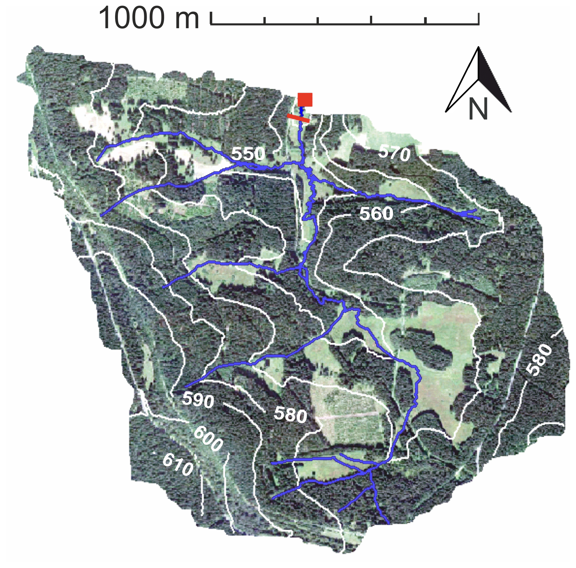
Figure 1 Topography of the Rappbode catchment with the UV-vis and discharge measurements at the outlet (red square). Transect for soil samples indicated by red line. Map data: ©Google, GeoBasis-DE-BKG.

2.2 Data basis

An overview of all variables utilized for site description and regression modeling as well as descriptive statistics of these variables are given in Table 1.

Table 1 Descriptive statistics of DOC and hydroclimatic variables. N refers to number of measurements; SD – standard deviation; Min – minimum of the measurements; Max – maximum of the measurements; CV – coefficient of variation. Class shows if the variable was utilized as response (r) or predictor (p) in statistical models.

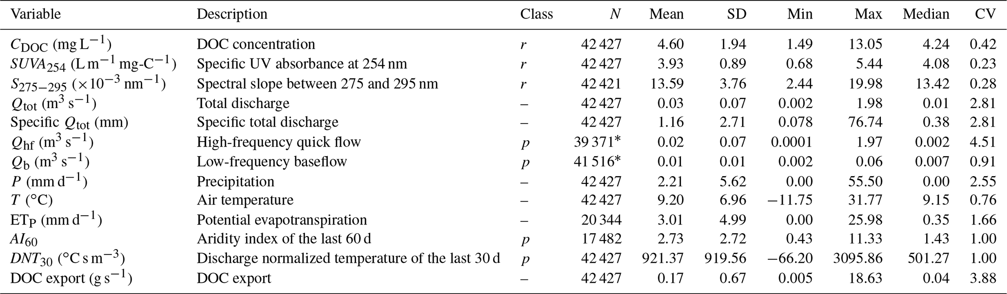
^* N of Q_b and Q_hf differs from Q_tot due to the applied filtering method for baseflow separation.

2.2.1 Monitoring of response variables: DOC concentration and quality

We used in situ absorption spectroscopy to estimate dissolved organic matter quantity and quality. For simplification and because carbon is the main focus of the paper, dissolved organic matter quality will be addressed as DOC quality in the following. DOC quality can be characterized by specific metrics based on the light-absorbing properties of dissolved organic compounds: SUVA₂₅₄ was calculated by normalizing the spectral absorption coefficient at 254 nm (SAC₂₅₄) for the corresponding C_DOC values. SUVA₂₅₄ correlates well with aromaticity of DOC and therefore can be used as an indicator of the general chemical composition and reactivity of organic carbon (Weishaar et al., 2003). To refine the understanding of DOC composition, the spectral slope between 275 and 295 nm, denoted S_275−295, was estimated from the adsorption spectra and calculated as described in Helms et al. (2008): a linear regression model was fitted for each time step to the logarithms of the absorption coefficients between 275 and 295 nm to derive the slope S_275−295. S_275−295 can help to distinguish between autochthonous and allochthonous DOC, molecular weights and processing (photobleaching and microbial degradation change aromaticity) (Helms et al., 2008). The general patterns of such DOC quality metrics can be used to infer information on origin and properties of DOC and thus to characterize source zones of DOC in riparian zones (Hood et al., 2006; Hutchins et al., 2017; Sanderman et al., 2009). An UV-vis probe (Spectrolyzer, scan Messtechnik GmbH, Austria) was installed in the stream (Fig. 1) from April 2013 to October 2014 to measure light absorption spectra from 220 to 720 nm in 2.5 nm steps every 15 min. There is a data gap from 11 December 2013 to 14 January 2014 due to general maintenance and recalibration of the UV-vis probe in the laboratory. Other gaps from 18 to 27 November 2013 and from 1 to 17 September 2014 were due to a probe failure; accordingly values were excluded a priori. Overall, the UV-vis dataset comprises 42 427 measurements. For a description of fouling correction, on-site probe maintenance and sampling procedure, refer to S1 in the Supplement.

After fouling correction, UV-vis measurements were used to derive C_DOC, SUVA₂₅₄ and S_275−295. For validation and calibration of C_DOC and SUVA₂₅₄, 28 grab samples were used that have been taken once every 2 weeks from the stream to measure the specific absorption coefficient at 254 nm (SAC₂₅₄ (UVT P200, Real Tech Inc., Canada). Subsequently, C_DOC was measured in the laboratory by thermo-catalytic oxidation at 900 ^∘C with nondispersive infrared (NDIR) detection (DIMATOC^® 2000, Dimatec Analysentechnik GmbH, Germany). A continuous time series of C_DOC from the UV-vis spectra was created using partial least-squares regression (PLSR) to the 28 concentration values via the R package pls (Mevik and Wehrens, 2007). The PLSR proved to robustly work with a large number of predicting variables and strong collinearities (Musolff et al., 2015; Vaughan et al., 2017). The procedure generally followed the method described in Etheridge et al. (2014) using all turbidity-compensated spectra within a single regression model, chosen by 10-fold cross validation of the training dataset. Through this method, C_DOC was defined by a local combination of several wavelengths that proved to yield better results than the predefined global settings provided by the probe (Vaughan et al., 2017).

SUVA₂₅₄ was calculated by dividing the spectral absorption coefficient at 254 nm (SAC₂₅₄) by the PLSR-derived C_DOC values. The resulting SUVA₂₅₄ values were then validated (but not calibrated) by the 28 SUVA₂₅₄ values derived from the manual SAC₂₅₄ measurements in the field and the associated lab C_DOC measurements (see Sect. 3.1). As a second quality metric S_275−295 was estimated from the fouling-corrected adsorption spectra as described above and in Helms et al. (2008). There are no laboratory values available to verify S_275−295 calculations, so calculated values were verified by comparison to the literature.

2.2.2 Predictor variables: stream level and discharge, evapotranspiration, and antecedent wetness condition

Discharge Q_tot was calculated from a stage–discharge relationship, which was established based on the 15 min stage readings from a barometrically compensated pressure transducer (Solinst Levelogger, Canada) and manual discharge measurements once every 2 weeks using an electromagnetic flow meter (n=42; MF pro, Ott, Germany).

Manually measured discharge maximum was 0.39 m³ s⁻¹ at a water level of 83.8 cm. Ungauged water levels above this value and the associated discharges were extrapolated from the stage–discharge relationship and found to be within a valid range when comparing to modeled discharge from the mesoscale hydrological model (mHM; Mueller et al., 2016; Samaniego et al., 2010). A hydrograph separation into event and baseflow components was applied following the method described by Gustard and Demuth (2009). Total discharge Q_tot was partitioned into a high-frequency quick flow (Q_hf) component, active during events, and a low-frequency component representing baseflow (Q_b). To derive the baseflow hydrograph, local flow minima of non-overlapping 5 d periods were selected and linearly connected to each other using the lfstat package (Koffler et al., 2016) in R (R-Core-Team, 2017). If the baseflow hydrograph exceeded the actual flow, it was constrained to equal the observed hydrograph of Q_tot. Consequently, subtracting the baseflow hydrograph (Q_b) from the total hydrograph of Q_tot yields the hydrograph of Q_hf, which has positive values during events (Q_tot > Q_b) and zero values during non-event periods (when Q_tot=Q_b). All consecutive positive values between two non-event periods (zero values) were considered one event and extracted from the complete dataset for further processing.

To characterize ambient weather conditions, a weather station (WS-GP1, Delta-T, UK) placed about 250 m northwest of the UV-vis probe provided data on air temperature (T), air humidity, wind direction and speed, solar radiation, and rainfall (P) at 30 min intervals. Measurements of the weather station started at 21 May 2013 until 26 November 2014. Measurements were at an hourly interval for the first 5 d, until 26 June 2013.

Potential evapotranspiration (ET_P) was calculated on an hourly basis from the weather data after the Penman–Monteith method (Allen et al., 1998). The antecedent aridity index (AI_t) gives an estimate of the water balance in the last t days and equals the aridity index for longer time periods given by Barrow (1992). Accordingly, AI₆₀ was derived for the measurement period by dividing the cumulative sum of precipitation over the last 60 d (P₆₀) by the cumulative sum of ET_P of the last 60 d (ET_P60). As a consequence, time series of lumped variables start t days after the actual begin of the field observations.

The discharge-normalized temperature of the preceding 30 d (DNT₃₀) was calculated by dividing the mean air temperature of the preceding 30 d by the mean discharge of the preceding 30 d. DNT₃₀ gives an estimate of the ratio between temperature (which controls soil DOC production; e.g., Christ and David, 1996) and discharge (which controls DOC export; e.g., Hope et al., 1994) in the last 30 d and therefore can potentially be related to the state of DOC storage in top soils. We chose AI₆₀ and DNT₃₀ as these variables turned out to work best in terms of variance inflation and interaction for the statistical modeling.

In order to obtain an analogous dataset, time series of all variables were constrained by excluding such observations that fell into the data gaps of the UV-vis probe (see Sect. 2.2.1).

2.3 Statistical analysis

Evaluation of the variable's predictive power was carried out for the entire dataset as well as for separated discharge events. Descriptive statistical tools were applied using the software R (R-Core-Team, 2017). Spearman's rank correlation was used to look for significant relations of C_DOC and DOC quality with potential controlling variables since concentration, discharge and solute loads in river systems usually have lognormal probability distributions while C–Q relationships can be described by power-law functions (Jawitz and Mitchell, 2011; Köhler et al., 2009; Rodríguez-Iturbe et al., 1992; Seibert et al., 2009).

2.3.1 Event-scale analysis

Consequently, concentration–discharge (C–Q) relationships were characterized and quantified in log-log space for the event analysis. Since metrics of DOC quality are typically normally distributed (Guarch-Ribot and Butturini, 2016; Sanderman et al., 2009), relationships between quality and Q_tot were analyzed in semi-log space. Corresponding C–Q and quality–Q relationships for each runoff event (n=38, extracted with the method explained in Sect. 2.2.2) were represented by combinations of multiple linear regression models with Q_tot, Q_b and Q_hf and their log transformations as predictors. As recommended by Marquardt (1970) and Menard (2001), multicollinearity of predictors was taken into account based on the variance inflation factor (VIF; R package car, Fox and Weisberg, 2011):

$$\begin{array}{}\text{(1)}& {\mathrm{VIF}}_i={\displaystyle \frac{\mathrm{1}}{\mathrm{1}-R_i^{\mathrm{2}}}}>\mathrm{10},\end{array}$$

where VIF_i is the variance inflation factor for every predictor variable i in the complete model, predicted by multiple linear regression from the remaining predictor variables of the complete model. $R_i^{\mathrm{2}}$ is the corresponding coefficient of determination. Predictor variables were excluded from the model if Eq. (1) holds for predictor variable i.

The best overall combination of two variables for the prediction of events was chosen according to the best mean R² of all 38 single models. Hence, independent variable log(C_DOC) is best predicted by a combination of both discharge components (log(Q_hf) and Q_b) during single discharge events. Subsequently, the 38 triplets of intercepts and regression coefficients of these single models were extracted for further analysis. Note that the hysteresis loop size did not significantly bias regression coefficients obtained from this method (S2, Fig. S1 in the Supplement).

2.3.2 Seasonal-scale analysis

To explain seasonal variations in the event analysis, the 38 regression coefficient triplets were correlated with seasonal-scale antecedent key controlling variables. Variables which showed strong correlations were added in different combinations to the existing event model as potential predictors for seasonal variations in addition to the event-scale variance. Here, models of the dependent variables (C_DOC, SUVA₂₅₄ and S_275−295) always used the same predictor variables. The interaction between two predictor variables was generally used for modeling. This implies that the measured hydroclimatic variables influence each other and thus cause a non-additive effect on the dependent variable. Here, we write interaction terms as the product between the two interacting variables (variable1 × variable2). Again, predictors (variables and interaction terms) were tested for multicollinearity and excluded from the complete model if Eq. (1) holds for variable i.

Akaike's information criterion (AIC) and R² were used for model selection and validation. The 5-fold cross validation was applied to estimate the prediction error. Once the most valid model was selected, the predictive power of the chosen predictors for the different models of C_DOC and DOC quality was tested. Partial models were built by stepwise dropping the least influencing predictors according to AIC and by comparing the subset of event-scale predictors with the subset of seasonal-scale predictors.

3 Results

3.1 Monitoring of DOC and hydroclimatic parameters

The basic statistics of UV-vis-derived C_DOC and DOC quality as well as hydroclimatic variables throughout the 1.5-year measurement period are given in Table 1.

The amount of precipitation during 2013 (665 mm) and 2014 (682 mm) was close to the long-term annual mean at the nearest weather station. Discharge shows event-type variability but in general followed the hydrological year, with the lowest values in late summer and highest values in spring (Fig. 2a). The highest discharge was 1.98 m¹ s⁻¹ during snowmelt on 27 April 2014. With a coefficient of variation (CV) much higher than 1, the discharge regime can be described as erratic (Botter et al., 2013), indicating the importance of the quick flow component for discharge in the Rappbode catchment. Consequently, the variability of Q_hf mostly follows Q_tot, but without the seasonal baseflow trends. A total of 38 discharge events have been separated by discharge partitioning, yielding an average frequency of 0.086 d⁻¹ (2.58 month⁻¹) at an average duration of 134 h per discharge event. A dry period occurred from 14 June to 23 July 2013, which resulted in a steady decline in discharge during that time (Fig. 2).

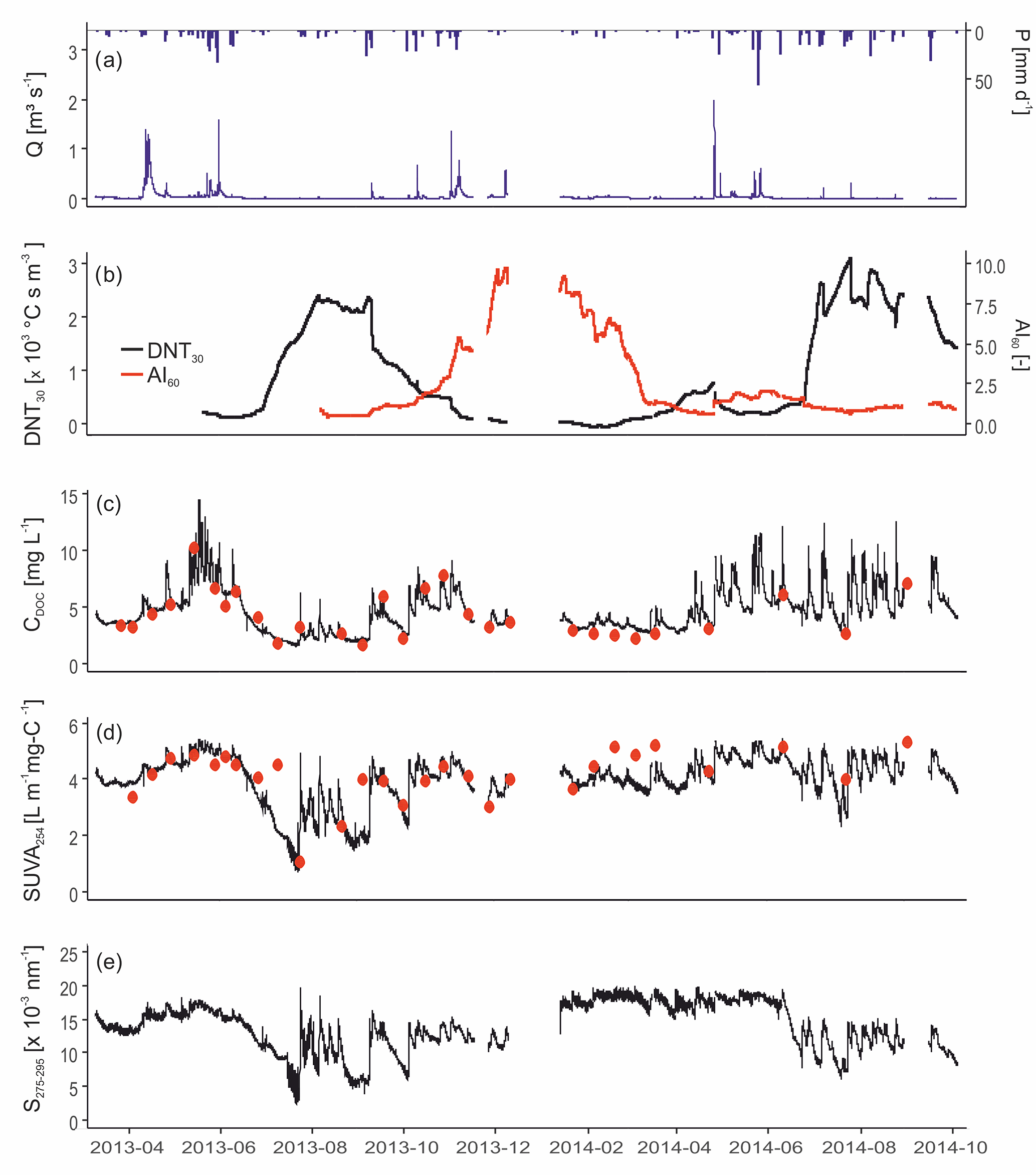
Figure 2 (a) Precipitation and discharge, (b) antecedent hydrometeorological conditions, (c) C_DOC, (d) SUVA₂₅₄ and (e) S_275−295 over the entire measurement period. C_DOC in (c) was fitted with PLSR to the measured grab samples (red dots). Grab samples (red dots) in the SUVA₂₅₄ values (d) were just used for validation.

Air temperature exhibited strong seasonal patterns and was comparable to the seasonal mean at the nearest station. Daily sums of ET_P peaked in summer whereas ET_P in autumn and winter reached the minimum. The general pattern follows a typical seasonal sinusoidal shape (not shown).

The aridity index AI₆₀ (median = 1.43) indicates a general wet climate with higher precipitation than potential evapotranspiration. AI₆₀ peaked in winter whereas minimum values occurred in summer during the drought and in winter during the freezing period (Fig. 2b). Summer precipitation has only a small impact on AI₆₀. With a CV of 0.74, ET_P60 generally has more influence on the variability of AI₆₀ than P₆₀ (CV = 0.53).

DNT₃₀ peaked in summer whereas minimum values occurred in winter (Fig. 2b). Generally, Q₃₀ (CV = 0.89) has more influence on the variability of DNT₃₀ than T₃₀ (CV = 0.53). Precipitation events in cold periods have only a small impact on DNT₃₀, and peaks due to precipitation are barely detectable.

C_DOC based on the PLS regression fits well to the DOC concentration measured in the lab (R²=0.97, residual standard error: 0.68 mg L⁻¹) (Fig. 2c). The maximum deviation of PLS-based C_DOC from lab-measured C_DOC was 1.7 mg L⁻¹ on 24 July 2013. We argue that the PLSR predicts the average characteristic composition of DOC rather well but hardly accounts for changes in DOC quality and thus spectral properties due to extreme situations like droughts and floods, which can strongly differ in DOC source area mobilization in comparison to average events (Vaughan et al., 2017). Accordingly, C_DOC and hence calculated SUVA₂₅₄ values match the manual measurements to a lesser extend during such situations, leading to an overall R² of 0.5 for SUVA₂₅₄ values, but removing three measurements taken during longer dry periods (9 July, 4 September 2013, 23 July 2014) increases overall R² to 0.73.

There are no laboratory values available to verify S_275−295 calculations, but calculated values are of the same magnitude as reported in the literature (Helms et al., 2008; Spencer et al., 2012).

C_DOC, SUVA₂₅₄ and S_275−295 exhibit pronounced event-type variability over the entire year (Fig. 2c–e). In winter months, DOC was low in concentration, but had a distinct quality signature with high S_275−295 and SUVA₂₅₄ values (Fig. 2c–e). Furthermore, only small fluctuations of concentration and quality were observed in winter. Summer months showed minimum C_DOC, SUVA₂₅₄ and S_275−295 values in both years during baseflow but also the most distinct C_DOC and quality variations during discharge events. Late summer and autumn C_DOC values were different between 2013 and 2014 with a pronounced temporal variability in 2014 compared to rather small fluctuations in 2013. DOC quality characteristics were similar in autumns of both years, exhibiting an average range compared to the entire measurement period. During events in spring and autumn, S_275−295 and SUVA₂₅₄ remained at a constant level, indicating the export of DOC of similar composition.

Exported DOC loads (Table 1) peaked during high-discharge events during spring and autumn and closely follow the hydrograph (Fig. S2). Accordingly, the CV of the load is closer to that of the discharge than to the CV of DOC (Table 1). Maximum DOC export was found during the discharge event on 27 April 2014 with rates of up to 18.6 g s⁻¹. Although events in drier summer months show stronger concentration fluctuations, exported loads remain low.

3.2 Correlation analysis

Table 2 gives an overview regarding correlations in the entire dataset. We used Spearman's rank correlation coefficient (r_s) correlation to determine the direction and strength of relationships between variables. C_DOC correlates strongest with SUVA₂₅₄, but r_s between C_DOC and S_275−295 and between S_275−295 and SUVA₂₅₄ is markedly smaller.

Table 2 Spearman's rank correlation coefficient (r_s) of possible controlling variables over the entire observation period. Only complete cases were used (n=17 082). All correlations are highly significant (p<0.001) because of the large sample size, r_s with absolute values larger than 0.6 printed in bold for better readability. Numerical subscripts of T, Q, AI and DNT indicate how many preceding days were aggregated.

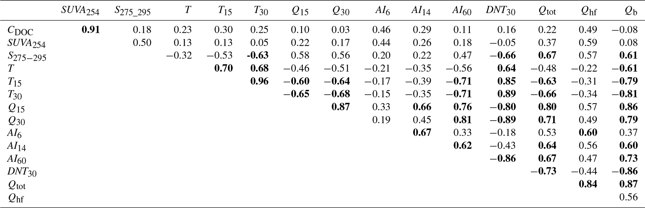
Correlations of Q_tot with S_275−295 are stronger than Q_tot with SUVA₂₅₄ and C_DOC. In comparison to Q_tot, correlations with Q_hf are markedly higher for C_DOC and SUVA₂₅₄, but lower for S_275−295. On the other hand, when relating C_DOC and metrics of quality to the baseflow fraction of discharge (Q_b), r_s is close to 0 for C_DOC and SUVA₂₅₄, but 0.61 for S_275−295. C_DOC and quality further correlate with antecedent discharge, temperature, discharge-normalized temperature (DNT₃₀) and aridity index (AI${}_{\mathrm{6},\mathrm{14},\mathrm{60}}$). C_DOC and SUVA₂₅₄ correlate best with AI₆, whereas S_275−295 correlates with T₃₀, Q₁₅, Q₃₀, DNT₃₀ and AI₆₀.

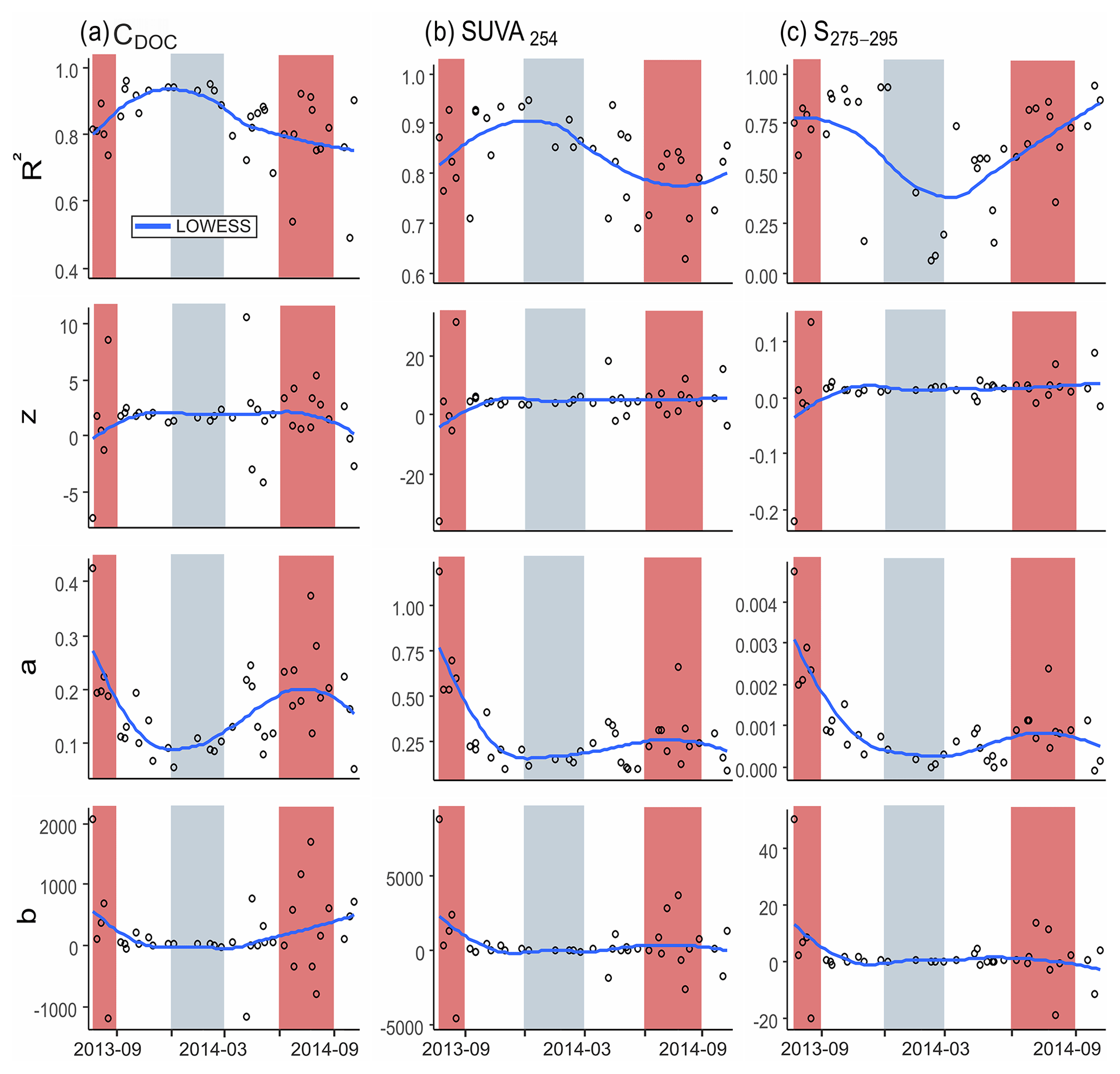
Figure 3 R², intercept z, and regression coefficients a and b of the model predictors log (Q_hf) and Q_b in Eq. (2) of all 38 events plotted against time. The headings in the top of the figure indicate which variable was represented by Y in Eq. (2). Blue lines indicate the locally weighted scatterplot smoothing (LOWESS), background colors indicate seasons (grey: winter; red: summer; white: autumn and spring). Note the different scales of the y axes.

3.2.1 Event-scale analysis

High coefficients of determination (R²) between C_DOC and DOC quality metrics with Q_hf and in the case of S_275−295 with Q_b underline the prominent role of discharge and its different timescales in DOC variability. Consequently, quantifying DOC mobilization for a range of individual events may provide information for better understanding direction, shape and strength of C–Q relationships. The analysis of the response of C_DOC and DOC quality to discharge events covers 44 % of the entire time series. The relationship between C_DOC and Q_tot during events resembles a segmented slope in log-log space (Fig. S3a), similar to the C–Q behavior described by Moatar et al. (2017), which inhibits a proper parameterization by the usually applied simple power-law regression. However, when detrending the discharge by baseflow subtraction, the resulting C_DOC–Q_hf relationship is more linear in log-log space (Fig. S3b). This behavior occurs for the event-scale discharge variability of the entire dataset. For DOC quality metrics SUVA₂₅₄ and S_275−295, we applied a similar model to predict the non-transformed independent variables:

$$\begin{array}{}\text{(2)}& Y=a\log \left(Q_{\mathrm{hf}}\right)+b{Q}_{\mathrm{b}}+z,\end{array}$$

where Y is log(C_DOC), SUVA₂₅₄ or S_275−295, and a and b are regression coefficients and z is the intercept.

We applied Eq. (2) to 38 individual discharge events. The mean R² of all log(C_DOC) models (one model for each discharge event) is 0.84 (±0.15). Respective mean R² values for SUVA₂₅₄ and S_275−295 were 0.83 (±0.14) and 0.64 (±0.26). Performance of the models is always better than a simple linear regression with log(Q_tot) (mean R² for log(C_DOC), SUVA₂₅₄ and S_275−295 is 0.76 (±0.16), 0.70 (±0.15) and 0.50 (±0.26), respectively). R² of the models from Eq. (2) varies over time (Fig. 3). Dependent variables log(C_DOC) and SUVA₂₅₄ show a similar behavior with maximum R² in autumn and winter and minimal R² values in spring and summer (Fig. 3a, b). R² values of the S_275−295 models show a different and less consistent pattern with higher variability between events than C_DOC and SUVA₂₅₄ models (Fig. 3c). In comparison to C_DOC and SUVA₂₅₄, S_275−295 values in winter and spring events have a systematically lower R².

Coefficients of C_DOC and DOC quality models vary between the events (Fig. 3a–c). Coefficient a (regression coefficient of log(Q_hf)) shows low but more systematic variations over time, represented by a smaller CV in comparison to z and b (mean CV_a=0.76, mean CV_z=2.58, mean CV_b=5.30 of the C_DOC, SUVA₂₅₄ and S_275−295 models). High a values indicate a stronger increase in C_DOC and change in quality of DOC with an increase in Q_hf, whereas small a values indicate only little change with increasing Q_hf. All three models show a distinct change in a from dry summer to autumn 2013. The summer months generally show the strongest variability in model coefficient, meaning that C_DOC and DOC quality reacted strongly and more variable to the comparable small discharge events. Winter months in contrast show the least variability in model coefficient a, indicating a more homogeneous reaction to discharge in this time of the year. Baseflow and intercept model coefficients b and z have a similar, less distinct pattern for all three models with higher parameter variability in summer compared to the other months.

3.2.2 Seasonal-scale analysis

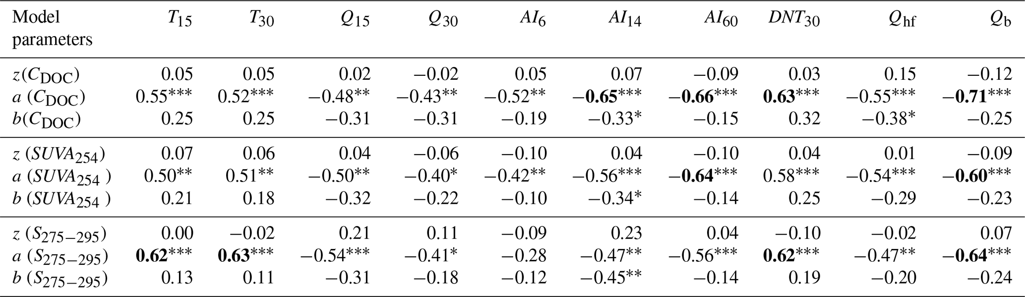
A correlation analysis of the model coefficients a, b and intercept z was performed to identify the variables that explain their temporal dynamics (Table 3). More specifically, we aim to predict a, b and z by hydroclimatic conditions before and during the event represented by the medians of DNT₃₀ and different temporal aggregations of AI, T and Q. Again, we rely on Spearman's rank correlation to characterize and quantify the relationships more independent of their shape. Intercept z as well as coefficient b (related to Q_b) do not show any correlation at p<0.001. Regression coefficient a (related to Q_hf) shows good correlations (p<0.01) with T₁₅, T₃₀, Q₃₀, AI₆₀ and DNT₃₀ for all models. But median values of DNT₃₀ and AI₆₀ are the only variables which show highly significant correlations (p<0.001) with coefficient a for C_DOC as well as for the quality metrics models. The strongest increase in C_DOC within an event (high a) occurs when AI₆₀ is low and DNT₃₀ is high, which translates into events during warm and dry low flow situations. On the other hand, during cold and wet high-flow periods (AI₆₀ and Q_b high, DNT₃₀ low), large events (high Q_hf) produce a smaller increase in C_DOC. This situation typically occurs during winter.

Table 3 Spearman's rank correlation coefficient (r_s) of the 38 C_DOC, SUVA₂₅₄ and S_275−295 model coefficients with hydroclimatic variables. Asterisks indicate p values (${}^{\ast \ast \ast }$: < 0.001; ${}^{\ast \ast }$: < 0.01; ^∗: < 0.05). r_s with absolute values larger than 0.6 are printed in bold.

Based on the highest r_s values in the correlation analysis for the event scale (Table 3), we selected DNT₃₀ and AI₆₀ as variables to explain seasonal variations in regression coefficient a. The results were used to build a regression model for all available data of C_DOC, SUVA₂₅₄ and S_275−295. We added to the model of Eq. (2) the seasonal-scale AI₆₀ and DNT₃₀. In addition we added those interactions for which VIF < 10 (Eq. 1): log(Q_hf) × Q_b, AI₆₀ × DNT₃₀ and DNT₃₀ × Q_b. These two additions allow the model to account for temporal changes in the relationships of C_DOC and DOC quality with discharge. Note that we, again, rely on power-law behavior of C_DOC but logarithmic (semi-log) behavior for SUVA₂₅₄ and S_275−295 (above):

$$\begin{array}{}\text{(3)}& Y=z+a\log \left(Q_{\mathrm{hf}}\right)+b{Q}_{\mathrm{b}}+c{\mathrm{AI}}_{\mathrm{60}}+d{\mathit{\text{DNT}}}_{\mathrm{30}}+i,\end{array}$$

where Y represents one of the three dependent variables log(C_DOC), SUVA₂₅₄ and S_275−295. a, b, c and d are regression coefficients, and z is the intercept. i indicates valid interaction terms (VIF < 10, Eq. 1) log(Q_hf) × Q_b, AI₆₀ × DNT₃₀ and DNT₃₀ × Q_b.

The results of the modeling are depicted in Table 4 and Fig. 4. A basic overview of all regression parameters and model statistics is given in Table S1. The C_DOC model performs best, explaining most of the overall variance ($R^{\mathrm{2}}=\mathrm{0.72}\pm \mathrm{0.04}$ 5-fold cross-validation prediction error), compared to the mean R² of 0.84 for modeling single events only. SUVA₂₅₄ and S_275−295 models explain similar parts (0.64±0.2 and 0.65±0.0) of the overall variance compared to the mean R² for the events of 0.83 and 0.64, respectively. All models generally explain both seasonal- and event-scale variability (Fig. 4, R²; see Table S2), but towards small values residuals of the DOC quality models tend to overestimate, whereas residuals of the C_DOC model increase with increasing concentration (Fig. S4). Yet, 95 % of the residuals lie within a range of 1.08 to −0.90 mg L⁻¹, ±0.44 L m⁻¹ mg-C⁻¹ and $\pm \mathrm{2.2}\times {\mathrm{10}}^{-\mathrm{3}}$ nm⁻¹ for the C_DOC, SUVA₂₅₄ and S_275−295 models, respectively.

Table 4 Evaluation of the whole dataset model by dropping the least influencing variable according to AIC, starting from the complete models (Eq. 3).

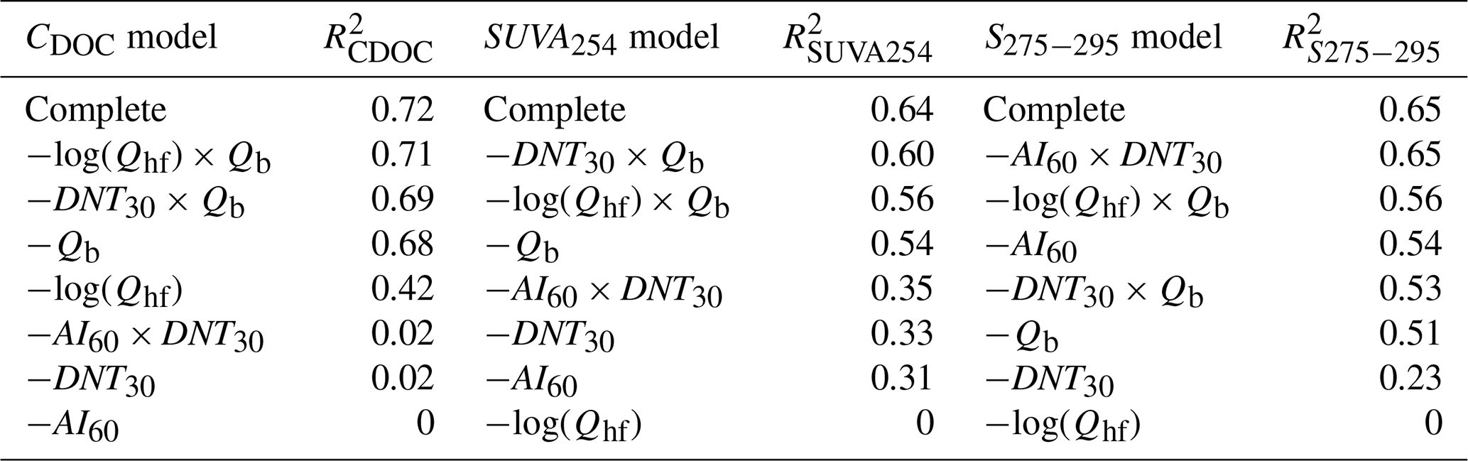
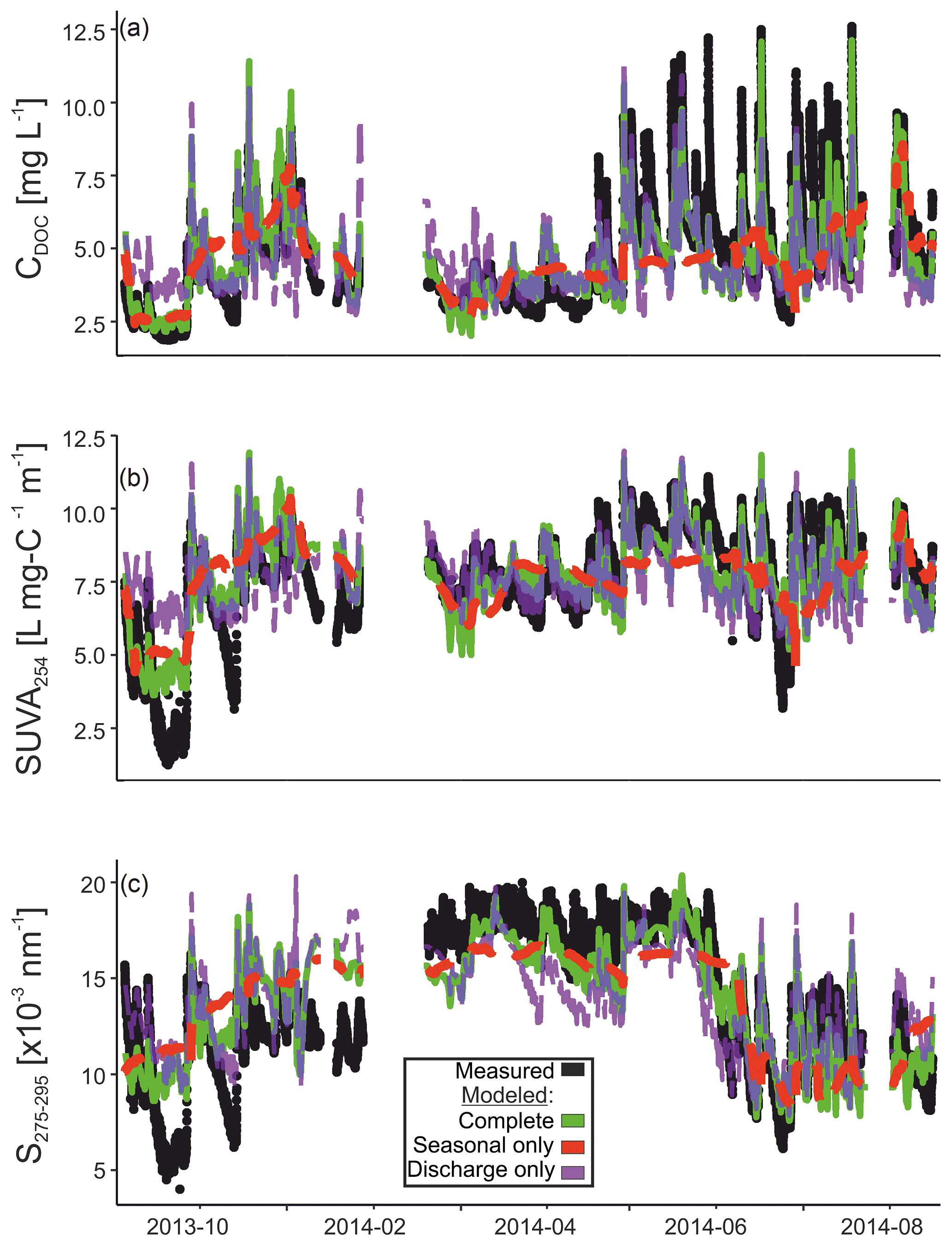
Figure 4 Comparison between measured (black) and multiple regression models of the complete predictors (green) as given by Eq. (3), only seasonal predictors AI₆₀ and DNT₃₀ plus their interaction (red) and only discharge predictors log(Q_hf) and Q_b plus their interaction (purple) for (a) C_DOC, (b) SUVA₂₅₄ and (c) S_275−295 values. Complete and discharge only model were smoothed (5-hourly) for better visualization.

Inspection of models taking only event-scale predictors (log(Q_hf), Q_b and interaction) or only seasonal-scale predictors (AI₆₀, DNT₃₀ plus their interaction) into account reveals that both sets of variables can explain a comparable part of the total variance (R² event scale: 0.40, 0.36 and 0.47; R² seasonal scale: 0.42, 0.36 and 0.48 for the C_DOC, SUVA₂₅₄ and S_275−295 models, respectively). Yet, when only using seasonal-scale drivers (AI₆₀ and DNT₃₀ plus their interaction), the general trend but no event-type variability is reproduced in the model (Fig. 4). On the other hand, the pure discharge model does not reproduce baseflow and peak height well during the seasons.

For the complete C_DOC and SUVA₂₅₄ model, seasonal-scale drivers AI₆₀ and DNT₃₀ plus their interaction DNT₃₀ × AI₆₀ and event-scale driver log(Q_hf) alone are the most important predictors, able to explain 68 % of the total variance for C_DOC and 54 % for SUVA₂₅₄ compared to 72 % and 64 % of the respective complete models (Table 4). In contrast to the C_DOC and SUVA₂₅₄ models, the interaction of seasonal-scale drivers (DNT₃₀ × AI₆₀) barely influences the R² of the S_275−295 model, but it is rather DNT₃₀ plus the interaction of DNT₃₀ × Q_b and event-scale hydrological drivers log(Q_hf) and Q_b that alone can explain 54 % of the variance compared to 65 % of the complete model.

Interactions between AI₆₀ and DNT₃₀ play a crucial role in the C_DOC and SUVA₂₅₄ models. There is a small negative effect of increasing soil wetness during low DNT₃₀ values and a small negative DNT₃₀ effect for dry soils. However, if exposed to increasing AI₆₀ values, the effect of medium and high DNT₃₀ values changes towards a positive interaction. Hence, when AI₆₀ is low and DNT₃₀ is high, which typically occurs during the summer months (Fig. 2b) or vice versa in winter, interaction leads to the lowest mean C_DOC and SUVA₂₅₄ values during non-precipitation periods (Fig. S5a, b). With medium AI₆₀ and DNT₃₀ values around autumn and spring, the interaction (Fig. S5c) has a more positive influence on C_DOC and SUVA₂₅₄ values, resulting in higher baseflow C_DOC and SUVA₂₅₄ values. This interaction can thus represent the change of regression coefficient a that was observed in the event analysis (Fig. 3). In comparison to the C_DOC and SUVA₂₅₄ models, for the S_275−295 model the interaction of log(Q_hf) with Q_b has direct influence on the time-variant regression coefficient a and thus more influence on the R² (Table 4).

There is a positive effect of increasing Q_b at low and medium log(Q_hf) values and a positive log(Q_hf) effect during low Q_b. However, the effect of log(Q_hf) changes towards a negative interaction if exposed to increasing Q_b so that log(Q_hf) barely increases S_275−295 values during high Q_b situations.

4 Discussion

4.1 Performance of event-scale and complete models

Within 1 year, DOC concentration and quality dynamics fluctuate on event and seasonal scales. The regression models revealed that discharge had a different impact on observed DOC concentration than on observed DOC quality in the Rappbode stream at the seasonal scale (Fig. 3). We found that during summer initial C_DOC was low during baseflow while large amounts of DOC were available to be exported from the riparian soils to the stream during events, leading to high model coefficient a (Fig. 3). Contrarily, the increase in concentration in winter is less pronounced (low model coefficient a, Fig. 3) because there is less DOC available to be washed out. Although the largest amounts of exportable DOC are to be expected at the end of the summer and in early autumn (Clark et al., 2005), C_DOC and DOC quality changed most distinctly with the discharge components Q_hf and Q_b in the summer (Fig. 3). Unfortunately, there were no DOC measurements of the riparian soil water available, which could further elucidate this discrepancy.

The regression models across the entire observed time series (Sect. 3.2.2) utilize event-scale drivers log(Q_hf) and Q_b as well as more seasonally driven variables AI₆₀, DNT₃₀ and their interactions to explain DOC concentrations and quality variations. We are aware that predictions based on statistical relationships between predictors and DOC responses, which are outside the range of the calibration data (e.g., during extreme droughts and flooding), have to be treated with care. Furthermore, validity and sensitivity of the statistical relationships to the predictors do not account for long-term changes in biogeochemical and hydroclimatical factors but can influence DOC export behavior on its own. Other influences not regarded in this model are the occurrence of chemical compounds like nitrogen (Garcia-Pausas et al., 2008), sulfate, chloride or acid deposition (Futter and de Wit, 2008), which all can impact the available forms, stability and mineralization of carbon in soils. Studying the interactions of DOC with other elements could therefore be useful to add understanding to the actual mobilization and processing mechanisms. But since we measured DOC in the stream, we view DOC as an integrated response signal, already carrying all the information from processing and transformation up to abiotic removal in the riparian zone. Thus, we argue that hydroclimatic and discharge dynamics as chosen here are a 1st-order controls of the DOC dynamics in the stream, represented by a high correlation coefficient (r_s) between hydroclimatic variables and DOC quantity and quality (Table 3) as well as an R² of 0.72 for the complete C_DOC model. Also, the complete C_DOC model represented the observed cumulative DOC export well with a Nash–Sutcliffe efficiency (NSE) of 0.998 throughout the year. Taken by themselves, seasonal-scale drivers (DNT₃₀ + AI₆₀ + DNT₃₀ × AI₆₀) were able to explain the same amount of C_DOC variability as hydrological event-scale drivers ($Q_{\mathrm{hf}}+Q_{\mathrm{b}}+Q_{\mathrm{hf}}$ × Q_b). But with an NSE of 0.979 cumulative modeled DOC export from event-scale drivers resembled actual cumulative DOC export much better than seasonal-scale drivers alone (NSE = 0.783), indicating that predictors based on low-frequency measurements alone are not able to explain DOC export as accurately as those derived from higher-frequency measurements. The different export behavior obtained from DOC export modeling based on low- versus high-frequency measurements is most pronounced during events (Fig. S6), which again highlights the importance of high-frequency measurements.

We used an hourly resolution for modeling C_DOC and DOC quality (∼17 000 values in ∼1 year). In a low-frequency study, Köhler et al. (2009) took 470 stream water samples in 14 years (based on Köhler et al., 2008). Consequently the DOC concentration variance, which needed to be explained, shifted from a focus on seasonal-scale and inter-annual variations in Köhler et al. (2009) towards highly frequent fluctuations on top of the seasonal-scale shifts and thus a more holistic perspective in the present study. In addition, Köhler et al. (2009) did not analyze the processes which are responsible for the shifts between the models, which had been independently set up for snow-covered, melting and snow-free periods.

Other studies took higher observational frequency into account and added DOC source characterization to better understand the mobilization dynamics: e.g., Broder et al. (2017) and Tunaley et al. (2016) examined event-driven changes in DOC export in a headwater stream, based on highly resolved (15 min to 3 h frequency) events. Like in the present study, both found that antecedent wetness conditions and seasonality are related to DOC dynamics in streams. Both studies provided a qualitative and descriptive assessment only and concluded that a more specific understanding of how DOC gets exported from catchments (Tunaley et al., 2016) might become even more important with respect to future changes in the hydrologic regime due to climate change (Broder et al., 2017). We argue that we need a better quantitative understanding of hydrological and biogeochemical mechanisms and interactions based on time series of different key controlling variables covering all relevant process scales in terms of resolution and length.

Several authors identified seasonality as an important driver for DOC dynamics (Ågren et al., 2007; Broder et al., 2017; Tunaley et al., 2016). However, the term “seasonality” is rather vague and often not clearly defined in terms of its impact on DOC export. This makes its use for a quantitative comparison between catchments and different climates difficult. Therefore we used a set of more easily identifiable, quantitative hydroclimatic variables instead, which reflect the general seasonal dynamics (Table 3) and at the same time allow for a better assessment of the dominant processes for DOC concentration and quality variations.

In summary, we used high-frequency measurements of hydroclimatic variables and their interactions as a proxy representation for seasonality, which allows a more quantitative comparison to other catchments and a more in-depth evaluation of the system.

4.2 Hydroclimatic classification

To estimate how event-scale and seasonal controls interact to produce the observed nonlinear responses of DOC concentrations and quality in our study catchment, we can separate the observation period into three distinct hydroclimatic states. These three discrete system states were chosen to highlight certain typical scenarios out of a continuum of hydroclimatical conditions, which are based on the seasonal-scale predictors of the complete regression models (Fig. 5): (1) high DNT₃₀ and low AI₆₀, representing warm and dry situations mainly found in summer; (2) moderate DNT₃₀ and AI₆₀, representing intermediate warm and wet situations, mainly found in spring and autumn; and (3) low DNT₃₀ and high AI₆₀, representing cold and wet situations mainly found in winter. To synthesize our modeling results in terms of potential underlying mobilization processes, these three states were compared by looking at both event and non-event responses of DOC concentrations and quality during those states.

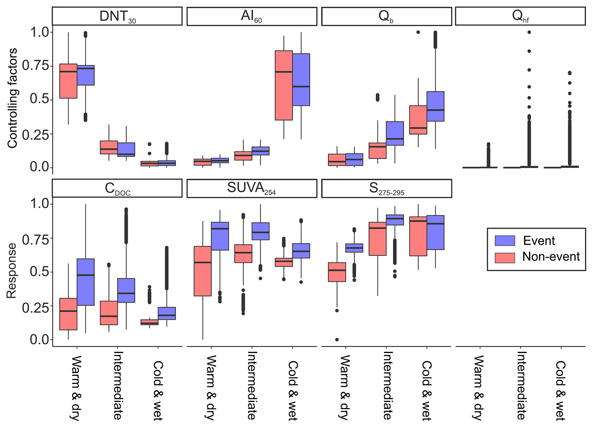
Figure 5 Box plots of hydroclimatic variables (controlling factors) and DOC quantity and quality metrics (response) classified into three hydroclimatic states: (1) warm and dry, (2) intermediate, (3) cold and wet. Red indicates non-event situations, and purple indicates event situations during the according states. Variables were rescaled for better illustration. Particular median C_DOC values during non-event situations were 4.13, 3.72 and 3.16 mg L⁻¹ for the warm and dry, intermediate, and cold and wet states, respectively. Both warm and dry and intermediate states differ highly significantly (Kruskal–Wallis test, p<0.001) from the cold and wet state.

Daily mean C_DOC, SUVA₂₅₄ and S_275−295 values of 1.49 mg L⁻¹, 0.68 L m⁻¹ mg-C⁻¹ and $\mathrm{5.0}\times {\mathrm{10}}^{-\mathrm{3}}$ nm⁻¹ were minimal at the end of the drought in August 2013, when baseflow levels were low, whereas values of 4.14 mg L⁻¹, 4.05 L m⁻¹ mg-C⁻¹ and $\mathrm{15.8}\times {\mathrm{10}}^{-\mathrm{3}}$ nm⁻¹ were measured during phases with higher baseflow levels in the cold and wet state. C_DOC, SUVA₂₅₄ and S_275−295 values showed the strongest increase during warm and dry situations (Fig. 5) also indicated by the highest slopes of regression coefficient a (event-scale models, Fig. 3). Events during the intermediate state also showed elevated C_DOC, SUVA₂₅₄ and S_275−295 values, but in comparison to summer events at a decreased variance and range (Fig. 5). Changes due to events in cold and wet situations were small in range and variance. Variance and mean of S_275−295 were generally lower during warm and dry situations than during intermediate and cold and wet phases. Therefore we conclude that seasonal-scale hydroclimatic variance controls the overall variance of S_275−295, whereas C_DOC and SUVA₂₅₄ are driven through event-type variance.

4.3 Conceptual model of DOC mobilization from the riparian zone

The relationship between AI₆₀ and DNT₃₀ in combination with differences in DOC concentration and quality of the three states is of particular interest to support a mechanistic explanation for differing DOC export during events. Hence, these metrics can be utilized for conceptualizing DOC mobilization dynamics of seasonal-scale variations in C_DOC and the observed quality–discharge dependencies (Fig. 6).

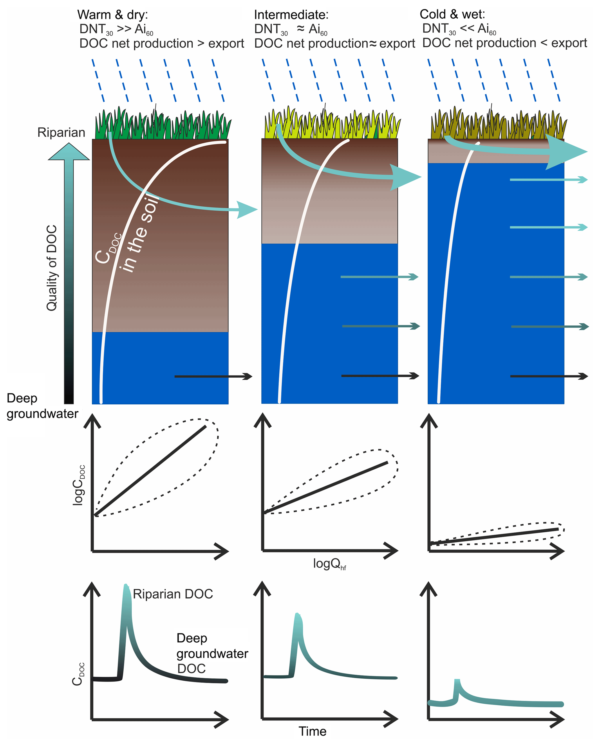
Figure 6 Conceptual model of riparian DOC export from precipitation during the three hydroclimatic states: warm and dry, intermediate, cold and wet. Depth of the soil column is around 0.5 m. Seasonal-scale variations in C_DOC in the soil solutions (summer vs. winter) were discussed in Kalbitz et al. (2000). Changing combinations between SUVA₂₅₄ and S_275−295 values are described as more groundwater-influenced (black) and more riparian-influenced (green) DOC quality. Arrows indicate the export of DOC; colors of the arrows refer to the respective DOC quality. Panels in the middle row show the relation between C_DOC and Q_hf during the three representative situations. Dashed lines indicate the “dispersion” of the point cloud (according R²) during the events. Panels in the bottom line indicate the change of C_DOC during an event. Corresponding changes of colors indicate more groundwater-influenced (black) and more riparian-influenced (green) DOC quality. Baseflow levels under cold and wet conditions are usually higher than baseflow levels during the warm and dry phase (see Fig. 5). Thus, during the cold and wet situation, higher layers of soil, more enriched in DOC, are activated, but at the same time, there is also a tradeoff between amount of water and available DOC in the respective soil layers which can account for lower overall DOC concentrations.

4.3.1 Warm and dry situations

Warm and dry situations are hydroclimatically defined by high temperatures and low mean discharge (high DNT₃₀), relatively dry soil conditions (low AI₆₀), and low baseflow levels, as typically found in summer when the Rappbode is fed mainly by deeper riparian groundwater. During baseflow conditions highly processed DOC enters the stream via the deeper groundwater flow paths (Broder et al., 2017). DOC in deeper groundwater has usually passed through multiple soil layers, and its amount and its composition has been altered by sorption and biogeochemical processes (Inamdar et al., 2011; Kaiser and Kalbitz, 2012; Shen et al., 2015). Low S_275−295 values indicate high molecular weight of DOC with a dominance of terrestrial waters (Helms et al., 2008; Spencer et al., 2012) entering the stream during that time. Precipitation events can get buffered and retarded in the soils (low Q_hf) (state warm and dry, Fig. 6). Due to the soil type and generally high groundwater tables in our catchment, soil moisture can remain high, even when there was no rainfall for some time. Yet, lower water contents can increase the mineralization rate compared to (oxygen-free) water-logged soils. However, Kalbitz et al. (2000) and citations therein report a positive correlation between mineralization rate and DOC concentration of the soil solutions. In consequence, DOC production can be higher than mineralization in the unsaturated riparian zone environment (Kalbitz et al., 2000; Luke et al., 2007) leading to a net production of DOC. Hence, favorable conditions for the accumulation of DOC during non-event periods exist in the subsurface due to the lack of moving water in the topsoil, where the high temperatures allow for (microbially driven) riparian DOC net production. To account for the positive balance between DOC removal mechanisms (mineralization, degradation) and DOC production in the riparian soil, we will use the term net production in the following.

We argue that the increase in C_DOC and change of DOC quality with discharge events is due to the addition of a new, distinct DOC source, located in the shallow riparian soils and connected via transmissivity feedback and preferential flow paths (Fig. S7). Since C_DOC during non-event situations was very low (Fig. 5), higher DOC concentrations exported from the topsoils with different quality were able to override the low-flow DOC signal towards a riparian zone signal. DOC quality during events changed markedly towards higher SUVA₂₅₄ values typical for higher aromaticity of the organic matter and associated with processed DOC (Hansen et al., 2016; Helms et al., 2008) and higher S_275−295 (but not as high as in cold and wet situation) indicating a relative increase in low-molecular-weight components in comparison to the low flow signal.

The (de)activation of an additional DOC source with changes in discharge could also explain the observed lower R² values in the event analysis during summer (Fig. 3) because in this situation C_DOC is not only driven by discharge but an addition of a differing DOC source that is not explained by the hydrological drivers of the event-scale models. The extent of this additional DOC source is determined by antecedent hydroclimatical conditions which favor DOC net production and thus indicate a sensitivity to biogeochemistry-driven DOC export as found by Winterdahl et al. (2016) on top of a general-transport-limited system (Zarnetske et al., 2018). Accordingly, event analysis showed the highest C_DOC and DOC quality peaks and revealed the steepest C_DOC–Q_hf and quality–Q_hf relations in summer. After the event, C_DOC and DOC quality metrics gradually drop back to the baseflow signal.

In contrast to our findings, Raeke et al. (2017) found higher-molecular-weight molecules at elevated discharge in three temperate catchments (including the one studied here). However, they used grab samples from different hydroclimatic situations and streams, thus potentially masking the event-scale dynamics of DOC mobilization as revealed in the current study. Also, the comparability between spectrophotometry and high-resolution mass spectrometry is questionable for DOC in general (Chen et al., 2016). But also the magnitude of in-stream processing and biodegradation could further influence DOC composition and hence SUVA₂₅₄ and S_275−295 measurements in stream water (Bernal et al., 2018; Hansen et al., 2016). However, Creed et al. (2015) and Nimick et al. (2011) stated that headwaters in general are dominated by allochthonous carbon with the role of in-stream processing increasing with stream order. Also, the role of in-stream processing at mean residence times below 1 d (which holds for our study site, 2 km downstream of the spring) was found to be minor (Kaplan et al., 2008; Köhler et al., 2002). Note that the wide riparian zone (several tens of meters) in our catchment consists of large parts of a flood plain, leaving only little possibility for leaf litter falling directly into the stream. Therefore, in-stream decomposition and leaf litter in the stream are likely to be of minor importance on our experimental site.

4.3.2 Intermediate state

Intermediate DNT₃₀ and AI₆₀ conditions are defined by moderate temperatures and discharge (medium DNT₃₀), precipitation, and evapotranspiration (medium AI₆₀), which results in higher baseflow levels compared to warm and dry conditions. Strong precipitation events translate into a distinct discharge signal (high Q_hf) (intermediate state, Fig. 6). Conditions for the accumulation of DOC during non-event periods are less favorable due to colder temperatures than warm and dry periods, decreasing the riparian DOC net production. During baseflow conditions some of the riparian DOC pools are already activated due to a higher groundwater table. This mixing of riparian and deeper groundwater DOC pools translates into intermediate values of concentration and quality parameters, even under non-event conditions.

In case precipitation increases discharge, the DOC signal changes both concentration and quality. This process happens faster than during the warm and dry situation since antecedent wet conditions facilitate DOC mobilization from riparian soils. Hence the temporal shift between DOC and discharge peak diminishes, resulting in higher R² values during events (Fig. 3). There was no exhaustion of the exportable DOC by consecutive events, although there is less DOC production paired with more effective export mechanisms, highlighting the large store of DOC in the comparably small riparian zone (Ledesma et al., 2015). The intermediate situation averages multiple situations (transition states in autumn and spring) and thus does not have the character and clarity of the end-members. Similar quality signals indicate the same process and location of source zone activation in autumn 2013 and 2014. However, concentration peaks developed differently, suggesting that the conditions for antecedent DOC storage and export during preceding phases were different. For example, there were only small mobilization and storage limitations during intermediate DNT₃₀ and AI₆₀ levels in spring 2014, which translated into pronounced DOC loads exported during events. However, DOC quality, especially S_275−295, barely changed during these events. Elevated temperatures during this period cause a warming of riparian topsoil, which is rich in organic matter, and hence an increase in biological processing and DOC production. Declining, still high baseflow levels and soil moisture lead to increased DOC production and export during these events.

4.3.3 Cold and wet situations

Cold and wet situations, mainly found in winter, are defined by low temperatures and high mean discharge (low DNT₃₀), humid conditions (high AI₆₀), and high baseflow levels (cold and wet state, Fig. 6). Generally low C_DOC values indicate that less DOC mass is available in relation to the generated runoff in the riparian zone in comparison to the warm and dry situations. Unfavorable conditions for the net production of DOC during non-event periods exist in the topsoil, where the low temperature impairs riparian DOC production. Accordingly, low SUVA₂₅₄ and high S_275−295 values were observed during that period, indicating a relatively higher amount of low-molecular-weight compounds due to reduced DOC processing. Furthermore, high baseflow levels lead to a good hydrological connectivity of DOC sources to the stream during non-event situations.

Precipitation events result in small slopes of the C_DOC and quality–Q_hf relationships. Dilution due to the impermeability of the frozen soil surface (Laudon et al., 2007) is likely to occur under prolonged periods of temperatures below zero. Since riparian DOC pools are already connected to the stream, we attribute the small shift in DOC quality and C_DOC during events to a shift of the contribution (hydrological connection) of DOC source areas with similar DOC quality, rather than to the activation of new, differing DOC pools. The 1st-order hydrological forcing under largely saturated soil conditions could thus explain the high R² but low regression coefficient a of the event-scale models of C_DOC and SUVA₂₅₄ (Fig. 3) in the cold and wet state. On the other hand, a dominance of hydrological forcing also implies little influence of antecedent biogeochemical conditions during this state (Winterdahl et al., 2016). In contrast to C_DOC and SUVA₂₅₄, R² of S_275−295 drops during the cold and wet situation, indicating a decoupling from hydrologic forcing. The dominant hydrological state could be able to leach differing DOC from the riparian zone by shifts in physicochemical equilibria (Shen et al., 2015), thereby forming the corresponding quality. However, this finding needs further research. The same observations of C_DOC and quality interaction during winter and spring (low DOC variance in winter, still low quality variance but strong C_DOC fluctuations in spring) were made in 2013. But due to the lack of weather data (the weather station was deployed 2 months after the sensor deployment, which inhibited derivation of AI and DNT for this period), no further statements can be made for this period (Fig. 2).

5 Conclusions

Seasonal- and event-scale DOC quantity and quality dynamics in headwater streams are dominantly controlled by the dynamic interplay between event-scale hydrological mobilization and transport (delivery to the stream) and inter-event and seasonal biogeochemical processing (exportable DOC pools) in the riparian zone. Observing DOC concentration and quality, together with hydroclimatical factors, at high frequency resolves dynamics at the temporal scale of the underlying hydrological and biogeochemical processes, which is unattainable with standard grab-sample monitoring. This allows for an improved, in-depth assessment of DOC export mechanisms as joint measurements of DOC quantity and quality give additional insights into source locations in the riparian zone, DOC processing and mobilization.

Observed DOC concentration, SUVA₂₅₄ and S_275−295 averaged at 4.06, 3.93 L m⁻¹ mg-C⁻¹ and $\mathrm{13.59}\times {\mathrm{10}}^{-\mathrm{3}}$ nm⁻¹, respectively, but were found to be highly variable in time. The analysis of event-scale variability revealed clear seasonal-scale shifts of the role of discharge in shaping DOC quantity and quality. Overall, the temporal dynamics of DOC concentration and quality can be explained by a few key controlling hydrological variables, which characterize instantaneous discharge, and hydroclimatic metrics, which define the conditions prior to the event.

The hydrological variables (Q_hf and Q_b) were able to explain 40 %, 36 % and 47 % of the overall variability of C_DOC, SUVA₂₅₄ and S_275−295 and play a crucial role in modeling DOC export. In comparison, seasonal-scale variables (AI₆₀ and DNT₃₀) alone are able to explain similar percentages (42 %, 36 % and 48 % for C_DOC, SUVA₂₅₄ and S_275−295) of the overall variability of DOC quantity and quality but lack in adequately predicting exported DOC loads. Combining both sets of variables, as done in this study, significantly increases the predictive capacity of the overall models (72 %, 64 % and 65 % for C_DOC, SUVA₂₅₄ and S_275−295). Evaluation of the developed statistical models also highlights the importance of interactions between the seasonal-scale antecedent predictors AI₆₀ and DNT₃₀ for DOC concentration and quality dynamics. AI₆₀ describes the potential for mobilizing DOC in riparian soils, whereas DNT₃₀ describes the changes in DOC storage by looking at the relationship of DOC production and prior mean export from riparian soils. Hence, the relationship between AI₆₀ and DNT₃₀ describes the potential for exporting DOC from riparian soils and allows us to conceptualize DOC exports under differing hydroclimatical conditions. We found that cold and wet situations (AI₆₀ high, DNT₃₀ low) are not mobilization limited (high mobilization potential due to wet soils and high baseflow levels) but limited in production and processing (due to low temperatures). High hydrological connectivity leads to low C_DOC when the DOC net production is low compared to the DOC export. Here, events do not change the quality signature of the DOC in the stream since all riparian DOC sources had already been connected to the stream before. In contrast, we interpret warm and dry conditions (AI₆₀ low, DNT₃₀ high) as mainly mobilization-limited situations (dryer soils, low baseflow levels). High DOC net production rates (high temperatures) and low hydrological connectivity lead to an accumulation of DOC in the upper soil layers of the riparian zone during non-event situations. Under those baseflow conditions low concentrations of highly processed DOC are exported from deeper soil layers to the stream. Overall, DOC quality varies the most during such warmer dry periods because events change the signature of DOC quality in the stream water by adding freshly processed DOC from upper riparian DOC sources to the older more intensely processed DOC from the underlying baseflow signature.

The findings reported and analyzed here provide a mechanistic explanation of the seasonally changing characteristics of DOC–discharge relationships and therefore can be utilized to infer the spatiotemporal dynamics of DOC origin in riparian zones from the DOC dynamics of headwater streams.

Our interpretation is based on the integrated signal of DOC concentration and quality measured in the stream. Accordingly, it remains partially unresolved, and the explicit processes in the riparian zone are responsible for the measured and conceptualized DOC dynamics in the Rappbode stream. Further research in the riparian zone with its shallow groundwater dynamics is necessary to fully mechanistically explain the explicit spatiotemporal mobilization patterns as well as to identify appropriate molecular markers that can be used to trace DOC from riparian source zones into the stream in order to better understand DOC mobilization processes.

The study demonstrates the considerable value of continuous high-frequency measurements of DOC quality and quantity and their key controlling variables in quantitatively unraveling DOC mobilization in the riparian zone. We believe our approach allows long-term DOC monitoring with a manageable allocation of time and resources as well as a better comparability between catchments of different seasonal characteristics. This study highlights the dependency of DOC export on hydroclimatic factors. Potential impacts of climate change on the amount and quality of exported DOC are therefore likely and should be further investigated.