the Creative Commons Attribution 4.0 License.
the Creative Commons Attribution 4.0 License.
 | 06 Dec 2019
Biogenic isoprenoid emissions under drought stress: different responses for isoprene and terpenes
Boris Bonn
Ruth-Kristina Magh
Joseph Rombach
Jürgen Kreuzwieser
Emissions of volatile organic compounds (VOCs) by biogenic sources depend on different environmental conditions. Besides temperature and photosynthetic active radiation (PAR), the available soil water can be a major factor controlling the emission flux. This factor is expected to become more important under future climate conditions, including prolonged drying–wetting cycles. In this paper we use results of available studies on different tree types to set up a parameterization describing the influence of soil water availability (SWA) on different isoprenoid emission rates. Investigating SWA effects on isoprene (C5H8), monoterpene (C10H16) and sesquiterpene (C15H24) emissions separately, it is obvious that different plant processes seem to control the individual emission fluxes, providing a measure to which plants can react to stresses and interact. The SWA impact on isoprene emissions is well described by a biological growth type curve, while the sum of monoterpenes displays a hydraulic conductivity pattern reflecting the plant's stomata opening. However, emissions of individual monoterpene structures behave differently to the total sum, i.e., the emissions of some increase, whereas others decline at decreasing SWA. In addition to a rather similar behavior to that of monoterpene emissions, total sesquiterpene fluxes of species adapted to drought stress tend to reveal a rise close to the wilting point, protecting against oxidative damages. Considering further VOCs as well, the total sum of VOCs tends to increase at the start of severe drought conditions until resources decline. In contrast to declining soil water availability, OH and ozone reactivity are enhanced. Based on these observations, a set of plant protection mechanisms are displayed for fighting drought stress and imply notable feedbacks on atmospheric processes such as ozone, aerosol particles and cloud properties. With increasing lengths of drought periods, declining storage pools and plant structure effects yield different emission mixtures and strengths. This drought feedback effect is definitely worth consideration in climate feedback descriptions and for accurate climate predictions.
- Article
(579 KB) - Full-text XML
-
Supplement
(2612 KB) - BibTeX
- EndNote


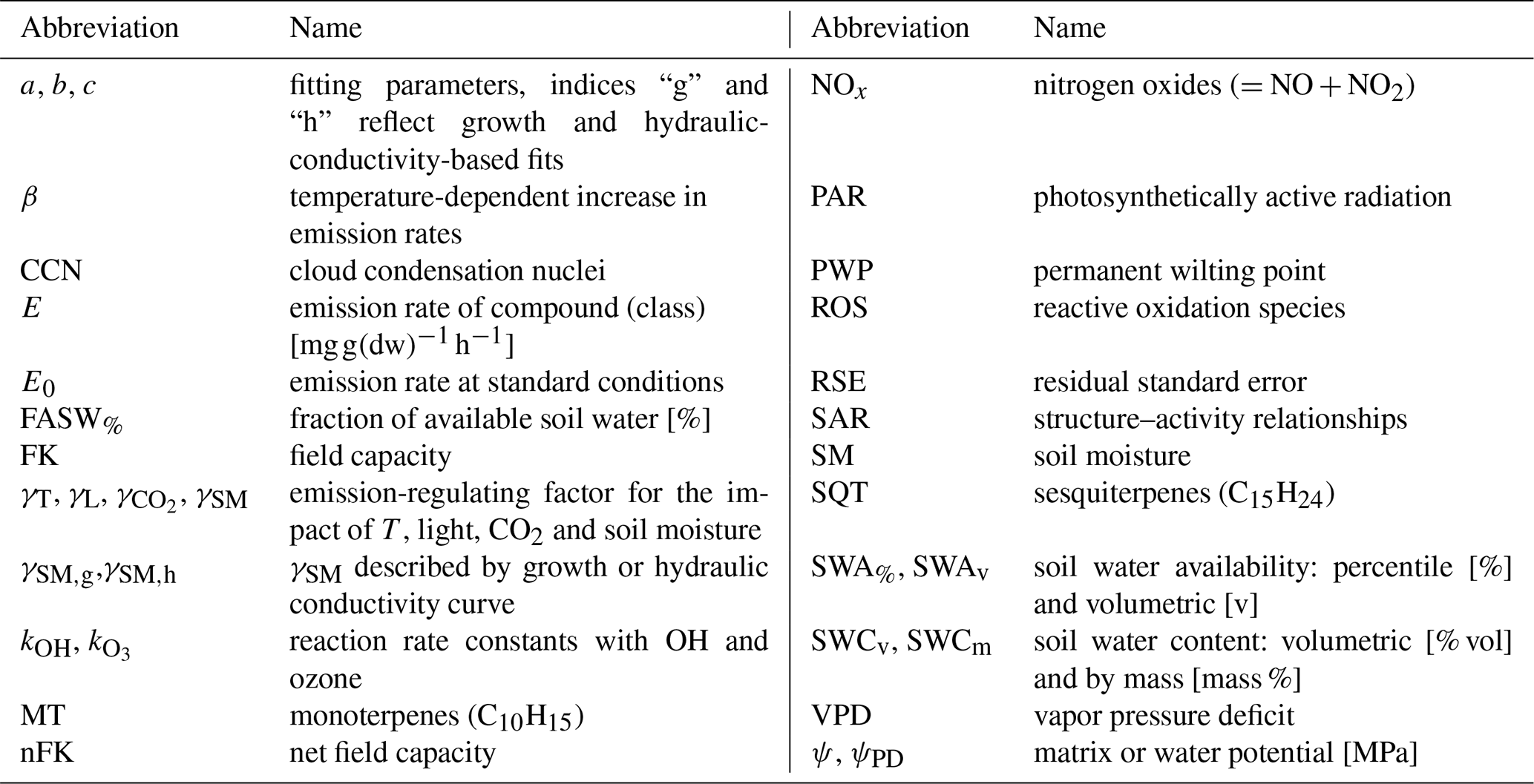
Emissions of biogenic volatile organic compounds (VOCs, E) are known to represent the largest contribution to global carbon flux besides carbon dioxide (CO2) (IPCC, 2014; Niinemets et al., 2014; Holopainen et al., 2017). The emissions and the corresponding deposition rates () are driven by the temperature of vegetation (Tveg) and soil (Tsoil), photosynthetic active radiation (PAR), ambient CO2 mixing ratio, defense against herbivores (Manninen et al., 1998) and reactive air pollutants (Bourtsoukidis et al., 2012), plant–plant communication and competition, fire, and drought (Lappalainen et al., 2009; Peñuelas et al., 2010; Guenther et al., 2012). The total amount of individual BVOC fluxes is linked to their production (de novo synthesis or online) and the storage (offline) capacities of individual plant types and species (Ghirardo et al., 2010) and is additionally affected by abiotic and biotic conditions. These include the temperatures of vegetation (Tveg) and soil (Tsoil), photosynthetic active radiation (PAR), ambient CO2 mixing ratio, defense against herbivores (Manninen et al., 1998) and reactive air pollutants (Bourtsoukidis et al., 2012), plant–plant communication and competition, fire, and drought (Lappalainen et al., 2009; Peñuelas et al., 2010; Guenther et al., 2012). While biogenic VOCs (BVOCs) represent a large variability of different structures and species (Goldstein and Galbally, 2007; Laothawornkitkul et al., 2009), it is commonly accepted that isoprene (C5H8) and monoterpenes (C10H16) display the majority (38 %–50 % and 30 %, respectively) of total BVOC exchange (1–1.3 Pg yr−1) (Goldstein and Galbally, 2007; Guenther et al., 1995, 2012) if methane is excluded. The exchange E is commonly described by the exchange at standard conditions E0 (T=30 ∘C) and scaled by factors for individual driving forces such as temperature (T), light (L) (Guenther et al., 1995, 2006, 2012) or soil water content (SWC), denoted here as SM in the index in accordance with the formulation of Guenther et al. (2006, 2012):
An overview of all the abbreviated terms and parameters can be found in Table 1. Some of the scaling factors of driving forces (γ) for exchange are reasonably well described regarding temperature and PAR, while other parameters like soil water availability (SWA) are mostly ignored due to a lack of understanding of influencing plant processes, although a simplified parameterization exists (Guenther et al., 2012). This neglect is confronted with changing climate conditions, such as warming of 0.15 ∘C every 20 years (Schölzel and Hense, 2011), with predicted increasingly long drought periods in Central European forest ecosystems such as the Black Forest in southern Germany (Keuler et al., 2016; Kreienkamp et al., 2018). So far, a single simplified formulation using a linear increase from no emission at the permanent wilting point (PWP) to maximum emission shortly above this point is commonly applied for different conditions. This is based on an experiment using poplar (Pegoraro et al., 2004a), analyzing isoprene only. The changing soil water conditions and the resulting change in BVOC exchange fluxes are expected to influence plant responses and protection capacities (Peñuelas et al., 2010; Rennenberg et al., 2006), the exchange following up ozone formation strength, and further climate feedback processes (Bonn, 2014). In this study we aim to investigate the individual behavior of isoprene, monoterpene (MT) and sesquiterpene (SQT) exchange fluxes and their correlation with SWA for available tree species to allow identification of processes controlling their emissions. As European beech (Fagus sylvatica), which is SWA sensitive (Gessler et al., 2007; Dalsgaard et al., 2011), is one of the most common tree species in Central Europe and of economic importance (Kändler and Cullmann, 2016), we will focus on the impact of the SWA effect on emissions.
2.1 Review of available studies and transfer between different water content parameters used
In order to develop an advanced description of the available water on BVOC exchange, available studies were collected, focusing on isoprenoid emissions in the context of different drought conditions. These studies include different tree types and several herbs, predominantly under controlled conditions and for selected compounds or compound groups (Table 2).
Lüpke et al. (2017a)Ormeño et al. (2007)Haberstroh et al. (2018)Hansen and Seufert (1999)Šimpraga et al. (2011)Rombach (2018)Lüpke et al. (2017b)Brilli et al. (2007)Pegoraro et al. (2004a)Fortunati et al. (2008)Bourtsoukidis et al. (2014)Ormeño et al. (2007)Lavoir et al. (2009)Bourtsoukidis et al. (2014)Pegoraro et al. (2004b)Table 2Overview of studies, tree species, and corresponding conditions, as well as soil water parameters used for deriving the γSM parameterization for isoprene, MT, and SQT emissions. References to the individual studies are listed in the final column. Soil water status parameters include the fraction of available soil water (FASW in %); leaf water content; available soil water (SWA% in %); soil water content by volume (SWCv), mass (SWCm), and ratio of water volume to soil mass (SWCvm); stem diameter; and water potential during daytime (ψ in MPa) and predawn (ψPD in MPa).
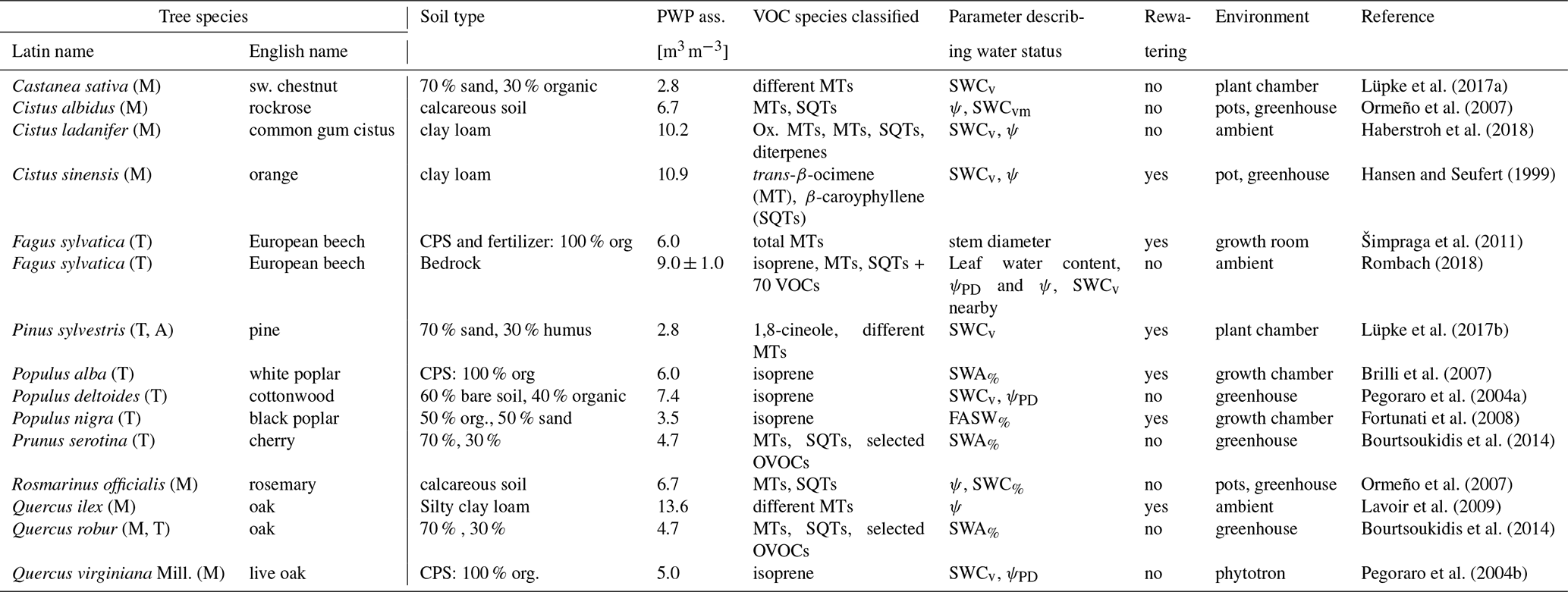
CPS: commercial potting soil (e.g., by Agrofino, Miracle Grow) including fertilizer or with additional fertilizer (Basacot); (A): arctic; (M): Mediterranean; (T): temperate.
2.2 Adapting available studies to a comparative scheme
2.2.1 Different conditions of individual studies
First, available studies on BVOC exchange for different tree species at different soil water conditions have been collected. It is important to note that these studies have been described in various ways using
- a.
different soil water parameters (SWA, SWCv and water matrix potential – Ψm),
- b.
different plant ages,
- c.
different soil types,
- d.
different lengths of investigation and time resolutions,
- e.
with and without rewatering,
- f.
different environments (laboratory, greenhouse and ambient).
The named different parameters complicate a direct comparison and include the assumption of an applicable transfer of laboratory or greenhouse experimental results with predominantly seedlings to ambient conditions, a transfer including notable challenges and questions as discussed, e.g., by Niinemets (2010a).
2.2.2 Different parameters used for describing the effect of soil water
The plants access to soil water is best described by the accessible water SWA (index “%”: fraction of accessible water, index “v”: volumetric amount) or by the suction pressure Ψm. Both parameters denote the soil water status and the ability of a plant to extract water from it (Blume et al., 2010). However, the easiest parameter to quantify soil water conditions by measurement continuously is volumetric SWC (SWCv). Therefore, SWCv has so far been used to estimate soil water effects on plant processes, e.g., by Guenther et al. (2006, 2012). However, different soil types possess different PWP preventing water being extracted by the plant below. Without the knowledge of the PWP of the soil investigated the information of SWCv to describe the plant water access remains incomplete and makes different studies difficult to compare. Therefore, we focus on SWA% as a primary parameter for describing the soil water effect and provide a set of equations to transfer between the different quantities. This makes different amounts of soil water comparable for different soil conditions and furthermore allows for easy usage in model studies that formerly used SWCv (Guenther et al., 2006, 2012). To support this, all parameterizations are stated by both, i.e., (a) by SWA% and (b) by SWCv. The SWA describes the amount of soil water above PWP ( MPa) up to field capacity (amount of water held by the soil against gravity, FK, MPa); this is called available or net field capacity (nFK) for the corresponding soil type and depends on the soil capacity to fix water (van Genuchten et al., 1980). Over the short term, SWA can exceed nFK (e.g., after an intense rain fall), but this excess water infiltrates the soil and is not available to the plant thereafter. A list of the different parameters used in the available literature is given and the transfer in between is assumed to be as follows (Blume et al., 2010):
FASW% and SWC% abbreviate the volumetric soil water content relative to its maximum value (field capacity FK). Converting water or matrix potential ψ values is a function of the actual soil mixture of clay, sand and silt, i.e., the different corn size distributions and classes and the inter-corn spaces available for water storage, which can be described by a water retention curve (van Genuchten diagram; van Genuchten et al., 1980; see e.g., Blume et al., 2010):
SWCv,r is the residual SWCv at completely air-dried conditions, SWCv,max is the SWCv at saturation, α the inverse of the air entry suction and n represents a measure of the pore size distribution. Representative data for different soil textures can be found, e.g., in Leij et al. (1996) and at http://soilphysics.okstate.edu/software/water/conductivity.html (last access: 17 January 2019).
2.2.3 Different soil types, corresponding PWPs and FKs
PWP and FK values for different soil types were calculated from the articles information based on data summarized by Chen et al. (2001) and their common soil type classification. Different soil types, predominantly expressed by different corn sizes (corn diameter Dp) and pore space volume, available for soil water, can be classified according to the contribution of sand (), silt () and clay (Dp<0.002 mm). Those mimic the potential of the soil texture to fix water, against which the suction pressure of plants needs to work for extracting soil water. This determines not only the PWP of the corresponding soil, i.e., the point at which a plant is unable to suck out any water of the soil pores, but also the maximum amount of water a soil can hold against gravity (FK or SWCv,max). The individual studies published refer to different soil types, PWPs and SWCv,max that need to be considered and included in a more general parameterization. Here, we use the contribution of individual soil types to the mixtures applied in the corresponding studies for calculating the PWP and the SWCv,max. In order to make different soil types and conditions comparable, all soil water describing parameters were converted to SWA% using PWP and nFK.
As this study is part of a beech and silver fir research project in southwestern Germany, most figures shown are displayed with two x axes, (i) the reference SWA% in percentage and (ii) an exemplary SWCv describing the one at the project's field site in Freiamt, southwestern Germany (Magh et al., 2018). This is representative for natural European beech soil common in Central Europe (Gessler et al., 2007) with a PWP of 4.7 % and a nFK of 31.2 %. In order to make results applicable to a wider range, any fitted equations take into account the soil properties and are provided for general conditions as functions of (i) SWA% (general reference) and of (ii) SWCv (requires adaptation to local conditions).
2.3 Different fitting approaches and corresponding driving forces
The effect of soil moisture on the emission of BVOCs is described by Guenther et al. (2006, 2012) using a three-step pattern: assuming (1) no emission below the PWP, (2) a linear increase in emissions between PWP (γSM=0) and PWP+4 % vol of SWCv (γSM=1), and (3) a soil-moisture-independent emission above the PWP. This empirical parameterization was based on isoprene emission measurements of Canadian black poplar (Populus deltoides) at their Biosphere 2 facility (Pegoraro et al., 2004a). A different suggestion, exponential dependence of emission on SWCv, was published recently by Genard-Zielinski et al. (2018) for isoprene emissions as well but for downy oak (Quercus pubescens) instead of black poplar.
For the overall soil moisture dependency of BVOC emissions at standard conditions (T=30 ∘C) several processes become important depending on the molecular size of the compound and its production, storage behavior, and water solubility.
- i.
Stomata-controlled effect. If the size of the BVOC molecule does not allow penetration of the leaf or needle surface layer, the last barrier between plant and atmosphere are the stomata. Thus, the emission process is controlled by stomatal opening behavior of the plant species (Simpson et al., 1985). Low SWA% and SWCv causes low Ψ; please note the negative scale, which triggers closure of stomata in order to increase the resistance for water molecules between leaf and atmosphere, helping to avoid loss of water by transpiration. Thus, γSM alters according to the hydraulic conductivity pattern (index “h”) given as
The curve starts at ah, i.e., the residual emitted fraction at PWP, and increases to unity as SWA% reaches 100 % at SWCv,max (FK). Both coefficients bh and ch determine the exact shape and slope of increase and are linked via
The shape is therefore different to the approach used in the MEGAN formulation (Guenther et al., 2006, 2012) as the effect sets in already below SWCv,max.
- ii.
Diffusion-controlled effect. If the emission can take place at least partially through the cuticula, in smaller chemical species for example, loss of plant water will cause a bending of the tissue surface. This will increase the cell pressure and influence conditions and forces of contained smaller BVOCs, leading to diffusion towards the ambient, i.e., emission. This process acts in a similar manner to biological growth processes and can be described by
Similar to the above examples, bg as well as cg represent curve shape parameters. The implicit γSM value at PWP, i.e., ag, is given by .
- iii.
Water solubility and transport effect. Further important processes, such as water-dependent productivity or transport (e.g., via sap flow), will display either a linear behavior or a mixture of Eqs. (4a) and (5). This depends on the limitations in the entire process chain from production, storage, potential transport and emission, which may be controlled by stomata opening or diffusion through the cuticula.
- iv.
Plant defense or interaction effect. Finally, a rise of BVOC emissions shortly above the PWP is apparent in some MT-related studies but are mainly seen in SQT-related studies. This may be explained by plant defensive strategies such as detoxification and reduction of radical oxidative species (ROS) species (Niinemets et al., 2014; Parveen et al., 2018; Piechowiak et al., 2019; Yalcinkaya et al., 2019), as most of these chemical species possess a high reactivity concerning ozone and radicals. The observations indicate an increase with decreasing SWA% or SWCv, until there is a rapid collapse close to PWP. We consider these observations as appearing to be like a gamma function with a maximum near the PWP, i.e., , with a set of parameters a, b, c and d characteristic for individual plant species. They may potentially reflect a species' ability to respond to oxidative stress.
2.4 Exemplary field studies: Application to ambient conditions
2.4.1 Plant nursery, Freiburg
A total of 11 examples of 8–10 year old Fagus sylvatica seedlings were studied in the plant nursery of the Chair of Ecosystem Physiology (48.014695∘ N, 7.832494∘ E) of the Albert-Ludwigs-Universität Freiburg with different soil water potentials, which were determined at predawn and during daytime between 19 and 31 July 2018. Six trees served as control plants, which were watered regularly, while rainwater was excluded by self-constructed roofs above the soil for the other five trees. The distance between the edges of control and stressed group were approximately 10 m with 1 m distance between individual tree stems. Water was added from a watering pot by moderate flows to each of the trees in order to control the amount of water and to minimize the effects on neighboring trees. Note that summer 2018 was extremely dry, with less precipitation (below 35 mm m−2 during June and July), which is only one-third of the 30-year average (90.5±40.5 mm m−2, Freiburg airport, distance: ca. 900 m NNW, German Weather Service, https://opendata.dwd.de/climate_environment/CDC/observations_germany/climate/monthly/kl/, last access: 15 July 2019) for those 2 months. Mean SWCv of control and stressed beeches were approximated by two methods: (i) the water potential of the experimental plants was determined with a Scholander pressure chamber (Scholander, 1966) at a cut branch before dawn and at around noon, and (ii) SWCv was estimated using measurements at a nearby field (ca. 600 m NW) with a similar soil structure (VWC, 10HS, Decagon, Washington, USA). BVOC emission was measured with the method described by Haberstroh et al. (2018). For this purpose, BVOCs emitted from beech leaves were collected during daytime using air-sampling tubes filled with Tenax (Gerstel). Analysis occurred with a gas chromatograph–mass spectrometer (GC-MS) system (GC model: 7890 B GC System; MS model: 5975 C VL MSD, with a triple-axis detector, Agilent Technologies, Waldbronn) equipped with a multipurpose sampler (MPS 2, Gerstel, Mülheim, Germany) (Magh et al., 2019). More details of the analysis can be found here (Kleiber et al., 2017).
Based on the observed emission rates and corresponding forest air composition, relative changes in OH and ozone reactivity of the emission cocktail observed were derived as follows (Nölscher et al., 2014; Mogensen et al., 2015). The sum of the individual products of emission rates [] and their corresponding reaction rate constants [] was calculated and compared to the related sum of the undisturbed reference trees. This includes the knowledge of a large set of compound reaction rates of which some are not obtainable in the available literature. Those have been approximated using structure–activity relationship (SAR)-based algorithms developed by Neeb (2000) and McGillen et al. (2011). In order to do so, the molecule of interest was split in its functional groups and the respective coefficients used for the estimate. As this approach is relative (i.e., disturbed to undisturbed trees), emissions of any vertical mixing are unimportant here but will have to be considered for the detailed impact on atmospheric chemistry, cloud properties and radiation (Seinfeld and Pandis, 2016), and the range of the impact. In this case, it is worth mentioning that forests usually extend over tens of kilometers in the Black Forest area. This indicates the importance of BVOC emissions in local atmospheric chemistry.
2.4.2 Black Forest conditions at Freiamt
SWCv values were measured at five different depths (5, 10, 25, 50 and 75 cm) with a time resolution of 2 h. Sensors were placed at different locations to test their heterogeneity, especially beneath different tree types, i.e., European beech (Fagus sylvatica), silver fir (Abies alba) and in between the two species. For further information about these measurements, see Magh et al. (2019). In order to approximate ambient SWCv effects on isoprene and terpene emissions, Eqs. (1), (4a), (5) and (10b) have been applied to meteorological measurements nearby and SWCv.
As indicated in Sect. 2.3, we standardized and tested the influence of available soil water on emission rates of isoprene (Eisop), MT (EMT) and SQT (ESQT) using different hypotheses: (a) a stepwise effect (Guenther et al., 2006), (b) a growth-rate-like behavior (Eq. 5), (c) a hydraulic conductivity pattern (Eq. 4a and b), (d) a stress defense response of SWA% (lower x axis) and, for comparison, the SWCv for a selected condition (upper x axis).
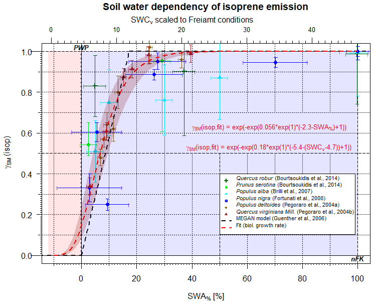
Figure 1Scaling parameter γSM(isop) for the effect of soil moisture on isoprene emissions as a function of SWA% (lower x axis) and, for comparison, the SWCv for a selected condition (upper x axis). Data points represent observations, and different colors refer to different studies. The dashed black line displays the approach by Guenther et al. (2006, 2012). The red line displays the present form.
3.1 Isoprene
Most studies of plant BVOC emissions affected by limited amounts of soil water have investigated isoprene. A summary plot of individual studies rescaled to comparable conditions is provided in Fig. 1. In Fig. 1, the corresponding SWA% conditions are plotted vs. γSM. The upper x axis of Fig. 1 displays typical SWCv representative of Black Forest conditions at the Freiamt site (PWP=4.7; nFK=31.2 %; soil: loamy sand; Magh et al., 2018). These conditions are similar to what has been found for European beech forest conditions elsewhere (Dalsgaard et al., 2011). Values of γSM displayed were obtained from measured emission rates (Pegoraro et al., 2004a, b; Brilli et al., 2007; Fortunati et al., 2008; Bourtsoukidis et al., 2014) and were divided by either (a) the corresponding measurements at well-watered standard conditions or (b) by literature values for the individual plant species. More information about the individual datasets and studies is provided in Table 2. Some values such as PWP and nFK are assumed according to the information provided by the authors of the corresponding studies. The figure clearly indicates that most of the studies focused on a specific smaller frame of the entire SWA% range, and only a single value has been measured below the PWP. This smaller range tended to yield a simplified description, e.g., the dataset of Pegoraro et al. (2004a), which was used by Guenther et al. (2006, 2012)(residual standard error (RSE)=0.163; r2=0.65). Testing different models for the dominating processes, the biological growth curve was found to fit the available datasets best (RSE=0.06).
Apparently, limited soil water access seems to influence isoprene emissions predominantly through growth stress and, to a lesser extent, stomatal opening, although growth stress and stomatal opening share similar features in a plot like Fig. 1, and the entire SWA% range allows discrimination between the two. Isoprene may diffuse out of the plant because of its smaller molecular size. Thus, a nearly closed stomata may not protect the plant from the release of isoprene because of enhanced cellular concentrations at reduced stomatal opening (Simpson et al., 1985; Fall and Monson, 1992).
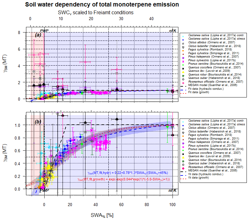
Figure 2Scaling parameter γSM(MT) for the effect of soil moisture on isoprene emissions as a function of SWA% (lower x axis) and, for comparison, the SWCv for a selected condition (upper x axis). The upper plot (a) displays the full data range, while the lower plot (b) zooms vertical area between 0 and 1.2. Data points represent observations, and different colors refer to different studies. The dashed black line displays the approach by Guenther et al. (2006, 2012) for isoprene only. The red line displays the present form using hydraulic conductivity as driving force, and the dark red line displays the biological growth stress as driving force.
3.2 Monoterpenes
The situation for monoterpenes (MT) is more complex, as different MT isomers display a different behavior with decreasing SWA% (and SWCv, Fig. 2). For example, in the case of European beech (Fagus sylvatica) the dominant MT sabinene (Moukhtar et al., 2006) declines drastically with reduced water availability, but limonene reduces to a smaller extent, whereas trans-β-ocimene stays constant within the uncertainty limit (Rombach, 2018). Lüpke et al. (2017a) report declines in α- and β-pinene, limonene, and myrcene emissions in response to increasing drought stress on Scots pine (Pinus sylvestris), while Δ3-carene emissions remained unaffected. An isotopic labeling test displayed a tendency for negatively influenced de novo production and contribution with declining SWCv and thus SWA%, while emission of stored monoterpenes was less affected. This may explain the overall behavior of MT emission and provide the storage pools to determine the total amount of emissions. If so, any damage to cell walls, or other plant structure elements, and extensive drought length will cause (a) a significant decline in total emissions beyond the drought period in the long term and (b) a decline in the ability of the plant structure to recover, form, and store new MT as before. Individual MT structure behavior, however, will depend on their detailed production pathway and storage location within the plant. Ormeño et al. (2007) describe an increase in MT emissions by rosemary (Rosmarinus officialis) at reduced soil water supply under Mediterranean conditions. The individual contribution of different structures even display a further process to be noted: the relative contribution of α-pinene increased at reduction of SWCv from 21 % to PWP, dropping thereafter in a similar manner to a stress response until cell damage was observed. A secondary contribution increase at very low SWCv values observed for sweet chestnut (Castanea sativa; Lüpke et al., 2017b) may result from changes in very small emission amounts and appears as a large uncertainty range awaiting further investigation. The remaining emission flux below PWP may result from de novo production or from different storage locations that are still functioning properly. Emissions of sabinene behave in a very similar way to those of α-pinene, while the fluxes of myrcene transiently increase around PWP. The opposite is true for cineole contribution that drastically declines with reducing SWCv and displays only at notable soil water presence. MT emissions of Aleppo pine (Pinus halepensis) display a pattern insignificantly influenced by γSM vs. SWCv for α-pinene, Δ3-carene and linalool, while β-pinene and myrcene tend to increase. Total kermes oak (Quercus coccifera) emissions of MT do not change significantly as well, but the contribution of α-pinene to total MT emissions enhances continuously even beyond the PWP. Therefore, the effect of individual MT structures depends on production rate as well as on storage pools and locations, which differ for different plant species. By changing the MT mixture, plants may adapt to different stress conditions for improved defense (more details in Sect. 3.5). However, the total MT emission effect of limited soil moisture seems to be more general.
A representative plot indicating the influence of SWA% on total MT emissions is shown in Fig. 2. The setup is identical to Fig. 1 for isoprene, i.e., the different studies included are marked with different symbols and colors. Lighter colors represent conditions after rewetting if performed in the same way as, for instance, for Scots pine (Pinus sylvestris) (Lüpke et al., 2017a). Lighter points indicate a severe plant structure damage and not entirely recovered plants reaching a lower emission intensity, as has been observed in several studies. Excluding those and assuming a soil water supply above PWP, different fits can be applied to the entire dataset. While all data scatter notably, the best performance is obtained with the hydraulic conductivity approach (residual standard error (RSE)=0.02), which is stomata-opening-controlled. Eventually the biological growth fit (RSE=0.14) works appropriately if the smallest values are neglected. However, the three-step approach by Guenther et al. (2006, 2012) used for isoprene fails (RSE=0.69) to appropriately describe the observations. Due to different capabilities of storing MT, commonly denoted as offline and temperature-driven emissions, the lower end of the fit displays a notable variance.
Note that the SWA% effect is less punctual at a specific SWA% than in the case of isoprene and the specific slope is soil-dependent, i.e., on nFK and PWP. The decline in emission strength already becomes larger than 5 % by 70±5 % of the accessible SWA%, depending on the fitting model chosen, not at about 6±2 in the case of isoprene, as also found by Guenther et al. (2012). However, the lower edge of the fitting is different but important, especially for arid regions and their corresponding emissions. On average about 22±5 % of the total MT emissions remain unaffected by soil water content (at PWP).
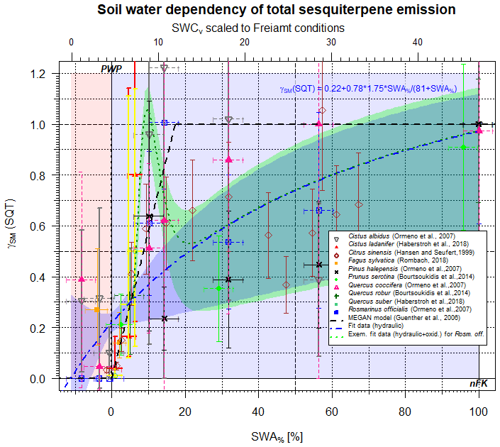
Figure 3Scaling parameter γSM(SQT) for the effect of soil moisture on SQT emissions as a function of SWA% (lower x axis) and, for comparison, the SWCv for a selected condition (upper x axis). Data points represent observations; different colors refer to different studies. The dashed black line displays the approach by Guenther et al. (2006, 2012) for isoprene only. The blue line displays the present form. The pointed green line represents an exemplary fit to γSM(SQT) based on Cistus and Rosmarinus officialis data.
3.3 Sesquiterpenes
Based on molecular properties, such as saturation vapor pressure (Seinfeld and Pandis, 2016), water solubility (Sander, 2015) and capability of being stored (Kosina et al., 2012), the effect of SWA% on the emissions of sesquiterpenes (SQT, C15H24) (Duhl et al., 2008) behaves the same way as seen for MT (Fig. 3), i.e., emissions are predominantly affected by plant hydraulic conductivity (RSE=0.153), which is controlled by stomatal opening. Applying the same approach as that for monoterpenes above, yields the following results for the soil moisture effect on total sesquiterpene emission rates γSM(SQT):
The onset of emission reduction with decreasing SWA% sets in even earlier compared to MTs (Rombach, 2018), as indicated by the different slopes in Fig. 3 and in Eqs. (9a) and (9b). However, individual structures reveal a large scattering at lower SWA% and thus SWCv values (<10 %) that are supposed to result from plant defensive strategies and mechanisms and perhaps from damage to cell walls and membranes.
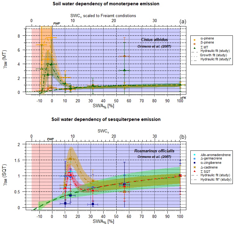
Figure 4Exemplary scaling parameter γSM for the effect of soil moisture with a maximum at PWP on individual and total terpene emissions as a function of SWA% (lower x axis) and, for comparison, the SWCv at Freiamt soil conditions (upper x axis) (Cistus albidus) (Ormeño et al., 2007). (a) SM effect on monoterpene emission fluxes of individual structured monoterpenes, as well as of the total sum of monoterpenes. (b) The same data as (a) but for individual structures and the total sum of sesquiterpene emissions (Rosmarinus officialis) (Ormeño et al., 2007).
3.4 Potential additional effects near the wilting point for terpenes
For some plant species, e.g., Cistus albidus and rosemary (Rosmarinus officialis), the effects of limited access to soil water on MT and SQT emission fluxes reveal a second maximum other than the one at γSM=1, appearing near the PWP (Figs. 4, S3–S8 in the Supplement). Highly temperature-stress-adapted and drought-stress-adapted species with the ability of to produce large amounts of terpenoids (e.g., Cistus ladanifer, Haberstroh et al., 2018, and Rosmarinus officialis, Ormeño et al., 2007) display a second maximum close to PWP not only for some MTs (Cistus ladanifer: d-limonene, myrcene, and trans-β-ocimene Haberstroh et al., 2018; Rosmarinus officialis: α-pinene and β-myrcene; Ormeño et al., 2007) but also for some SQTs and diterpenes (DT) (Cistus ladanifer: α-cubebene, α-farnesene, ent-16-kaurene, and β-chamigrene Haberstroh et al., 2018; Rosmarinus officialis: Δ-cardinene and α-zingiberene Ormeño et al., 2007, Fig. 4) and even the sum of all species. This is apparent, for instance, in the studies of Ormeño et al. (2007) and Haberstroh et al. (2018) of a broader range of plant species. As can be seen in Figs. S3–S8 in the Supplement, there is a statistically significant difference between individual chemical structures for different plant species, indicating a specifically adopted plant species. If those plots are investigated in more detail it is apparent that, for example, the monoterpene α-pinene increases with decreasing SWA% for Rosmarinus officalis (S6) and Quercus coccifera (S5) but persists for Pinus halepensis (S4) (Ormeño et al., 2007). The emission of the monoterpene β-pinene is declining for Cistus albidus (S3), stays put for Rosmarinus officialis (S6), and enhances for Pinus halepensis and Quercus coccifera. Similar observations can be made for SQT emissions with SM values near the PWP: Δ-cadinene emissions increase with decreasing SM, while α-zingiberene emissions decline for Rosmarinus officialis. Haberstroh et al. (2018) monitored decreasing emission fluxes for all of the individual chemical SQT structures for Cistus ladanifer and Quercus robur in a very narrow SM range (SWA%=ca. 0 %–6 %). This is the opposite of the behavior of Cistus albidus (Ormeño et al., 2007). Δ-germacrene emissions tend to increase near the PWP for Cistus albidus, Quercus coccifera and Rosmarinus officialis (Figs. S3, S5 and S6).
The enhanced emitted chemical species are known to possess a substantially higher reactivity with respect to ozone, which is usually elevated at drier conditions on longer timescales because of enhanced production rates and accumulation (see Sect. 3.7). For example, α-pinene possesses an O3 reaction rate constant () of , compared to those of β-pinene and Δ3-carene of and , respectively (Atkinson et al., 1990). With respect to the OH reaction, β-pinene reacts faster ( ), followed by α-pinene and Δ3-carene, with corresponding rate constants kOH of and , (Atkinson and Arey, 2003). This can be extended for other monoterpenes if more data is available, especially for d-limonene, terpinolene and other very reactive MTs. However, the amount of data for individual species is quite limited and depends on different plant ages, which does not allow for deriving a trustworthy equation at this stage. Sometimes the number of data points is equal to the number of parameters to constrain. The situation looks similar for SM effects on SQT emission rates. Consider, e.g., the bottom plot for SQT in Fig. 4, displaying allo-aromadendrene, Δ-germacrene, Δ-cadinene and α-zingiberene. Reaction rate constants with respect to ozone are , unknown, and unknown, respectively. The corresponding kOH for OH reactions are for aromadendrene, with further reactions not accessible based on experiments. However, structure–activity relationships such as that from US EPA (2018), indicate constants of ca. 10−10 . Thus, we assume this secondary maximum to occur as detoxification and defensive strategies of the plants (Kaurinovic et al., 2010; Höferl et al., 2015). Because of notable variations in measurements, this effect is not significant for all the Mediterranean species but only for the Cistus ladanifer and Rosmarinus officialis measurements. To incorporate this feature near the PWP exemplarily, which tends to be linked to higher ozone concentrations, this secondary maximum can be taken into account using a gamma function term added to the hydraulic conductivity curve (RSE=0.147) in Eq. (10a) and (10b):
a, b, c and d state parameters for the individual response of plant species to severe drought stress (gamma function), and they need to be adapted to the exact plant or ecosystem response studied on the local scale. An example is shown by the green line in Fig. 3 (applied parameters in here for Cistus ladanifer and Rosmarinus officialis: a=0.4; b=1.57; c=0.6; d=1). It is of interest that different structures seem to behave differently according to their historical stress adaptation, as presented by Fortunati et al. (2008) and Lüpke et al. (2016). In contrast to the hydraulic-conductivity-related description, the stepwise approach (Guenther et al., 2006) applied for isoprene fails at reproducing the declining pattern accurately (RSE=0.895).
3.5 Further BVOC emission rates
In addition to isoprene, MT and SQT, other VOCs are released by plants in notable amounts, but the impact of soil moisture on them is even less studied. Because of the huge number of different oxidized species and related publications, including those within the parameterization would extend this study greatly. A snapshot of individual correlation coefficients of different compound groups and species can be seen in Fig. S1. A non-negligible role of those larger VOCs seems plausible, either via formation pathway or oxidation processes within the plant. Those species supply further molecules that can buffer oxidative stresses onto the plant's internal processes. Additionally, they have substantial implications especially for OH reactivity (Atkinson et al., 1990; Atkinson and Arey, 2003; Neeb, 2000; Müenz, 2010; Seinfeld and Pandis, 2016; US EPA, 2018). Overall, there is a tendency (Rombach, 2018) for an increased total BVOC emission under drought-stressed conditions, but there is a large scatter of individual species reactions. However, the implications for OH reactivity and thus atmospheric chemistry are of relevance, as this parameter describes the plant's ability to still counteract oxidative damages by BVOC emissions.
3.6 Effects on reactivity
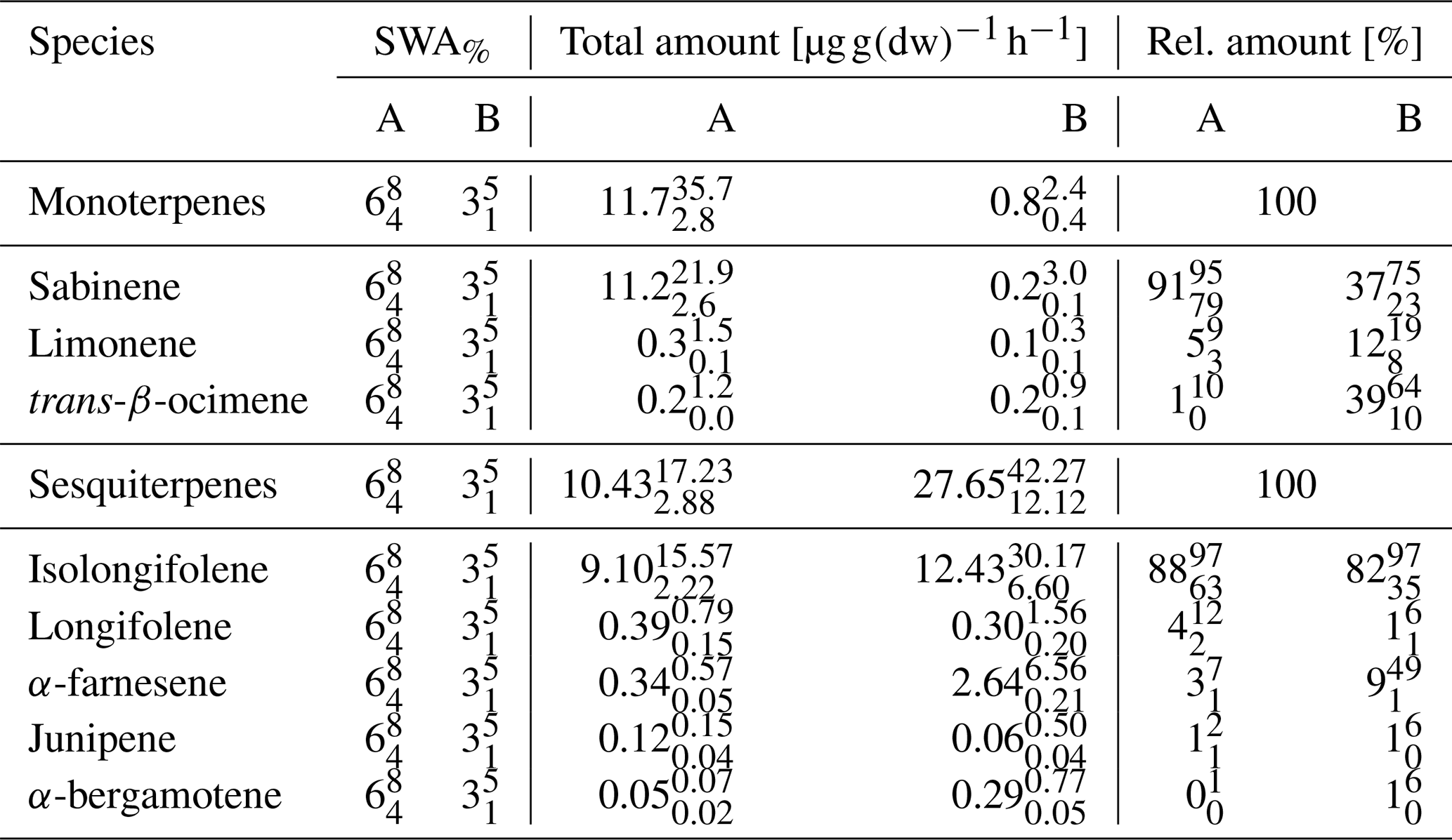
As chemical oxidation and ROS cause substantial damage to plants (Loreto and Velikova, 2001; Oikeawa and Lerdau, 2013), especially at stressed conditions such as warm and dry conditions, any strategy of plants to counteract or detoxify will be beneficial for survival and plant competition. An indication for this may be seen in the local emission increase in SQT near PWP for some plant species. Saunier et al. (2017) found a stable ratio of catabolic to anabolic BVOC emissions, i.e., emission fluxes related to oxidation stress and to non-oxidative stress production, respectively, during recurring drought periods for downy oak (Quercus pubescens) at Mediterranean conditions. This is different for different plant types and their adaptation to stress conditions (Niinemets, 2010a, b), i.e., the need to compensate for oxidative stress for survival. Looking at the pattern of absolute and relative MT and SQT emissions with declining SWA% values, it becomes obvious that more reactive structures tend to increase until plant cell damage occurs (Ormeño et al., 2007; Bourtsoukidis et al., 2012; Nölscher et al., 2016). SQT emissions displaying this transient peak around PWP especially cause a remarkable change. For example, reducing the SWCv for European beech by approximately 3 % vol close to PWP increases the total emission of SQTs by 170 %. The individual SQT species, however, show different patterns (Table 3). While emission of junipene declines (−50 %), those of longifolene stays constant within the uncertainty limits and the corresponding fluxes of isolongifolene, α-bergamotene and α-farnesene increase drastically (+50 %, +500 % and +700 %). Other VOCs analyzed (total: 81 VOCs; Rombach, 2018) operate in various ways: sabinene emission nearly vanishes at PWP. In contrast, emission of α-terpineol increased. Overall, the total emissions of VOCs and C increased tentatively (Fig. 5). This caused total OH reactivity and especially ozone reactivity to tentatively enhance (OH: %; O3: %) at a SWCv change of approximately 3 % vol. In this way the total amount, the changing composition and reactivity provide a tool for plants in this example for European beech to counteract oxidative stress and damage. The median change in OH reactivity corresponds nicely to the increase in total carbon emitted, as most organic species react with OH. However, the change in ozone reactivity is primarily related to the changes in individual SQT emissions. The large uncertainty in this context results from partially unknown reaction rate constants estimated either from similarity or from structure–activity relationships (SAR) (Neeb, 2000; McGillen et al., 2011). Since the storage pools, especially of larger terpenes, will be depleted with prolonged duration of drought, this effect will weaken over time.
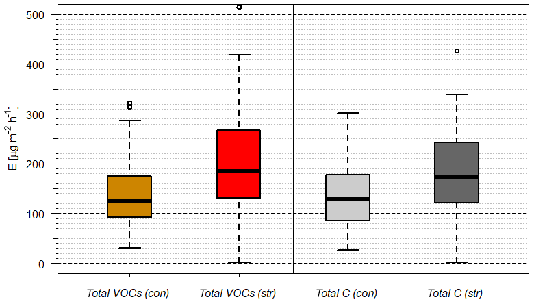
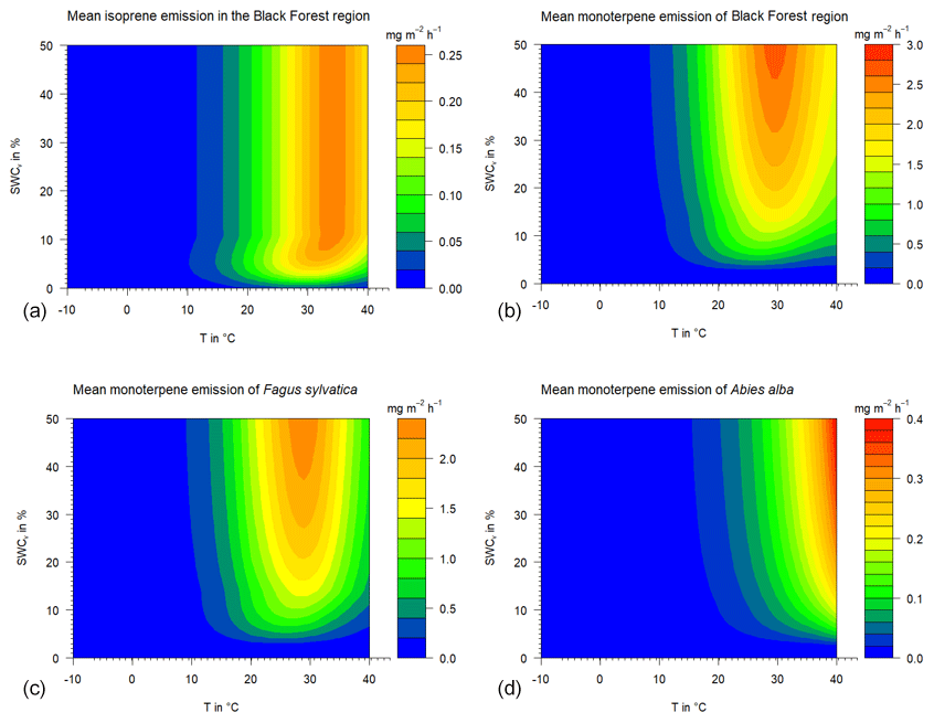
Figure 6Calculated mean isoprene and monoterpene emissions under different temperature and drought stress conditions using the parameterizations of Guenther et al. (2012) and the SWC dependency derived in this study. “Black Forest region” represents the forest inventory mean tree species mixture of the Black Forest area: (a) total isoprene emission, (b) total monoterpene emission, and baseline Fagus sylvatica and Abies alba MT emission rates (c and d).
3.7 Application to atmospheric conditions: ambient SWCv and its effect on emission rates at the reference site
In order to test the impact of the described effects of SWA% and thus SWCv on isoprenoid emissions, we apply the following emission flux parameterizations for isoprenoids from European beech and silver fir, which were quantified in earlier studies in this region excluding the SWA% effect (Moukhtar et al., 2005, 2006; Šimpraga et al., 2011; Bonn et al., 2017).
SM effects on specific emission rates have been calculated by including and excluding the individual γSM factors as multiplicands on the results. In Eq. (11a–f) CT and CL abbreviate the temperature- and light-scaling factors of Guenther et al. (1995), as well as TL the temperature of the needle or leaf surface in ∘C.
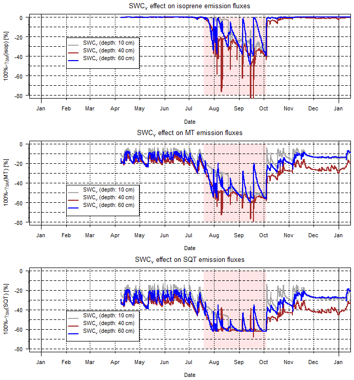
Figure 7Calculated γSM effects during 2016 at Freiamt on isoprene, total MT and SQT emission rates. Note that there were two induced drought periods during the summer and quite saturated conditions otherwise. The applied drought period is indicated by a reddish background.
The base effect of soil water on isoprenoid emission rates can be exemplarily shown assuming a temperature of 30 ∘C, i.e., standard conditions (see Fig. S2 in the Supplement). The available soil water for a plant has different impacts at distinct SWA% values. At a SWA% (i.e., SWCv (Freiamt)=20 %) of 35 %, isoprene emission rates display no decline, while the corresponding rates of MT and SQT reduce by 15 % and 25 %, respectively. Assuming an SWA% of 10 % (SWCv=10 % with a PWP of 4.8 % at Freiamt), isoprene, MT and SQT emission rates represent only 95 %, 50 % and 40 % of the standard rates, respectively. Therefore, the amount of soil water has the strongest effects on the larger terpenes, shrinking with molecular size. Isoprene emissions will stay unaffected longer than MT and will keep ozone production high if isoprene is the dominant class of isoprenoids released by the ecosystems in the nearby region. Depending on the tree-specific emission, i.e., online- and offline-including temperature effects, different locations of emission optima or maxima are found (Fig. 6). The predominantly de novo-emitting European beech will emit the most close to 30 ∘C, while the maxima of silver fir emission rates are shifted to larger temperatures. Similarly, the effects of changing SM will occur at the very same temperatures.
The overall impact of variable SM pattern on isoprenoid emissions was investigated using exemplary SWCv data at five different depths. Those measurements were located within the reference stand of a European beech (Fagus sylvatica, Fs) and silver fir (Abies alba, Aa) of the BuTaKli project in Freiamt within the Black Forest (southwestern Germany) region (Magh et al., 2018). In general, the uppermost layer dries out fastest, especially during summertime, while lower layers, i.e., below 30 cm, retain a higher SWCv for a longer time period. This implies different effects on the tree species with different rooting depths and thus access to soil water. Regarding the effect of SM on isoprenoid emissions, i.e., the γ factor, the γSM values for one vegetation period (during 2016) are shown in Fig. 7. Individual plots represent the SWCv emission effects of different compounds or compound classes and different colors illustrate the SWCv-based values for three different depths. Apparently during summertime, when the evapotranspiration flux and the emission rates are highest due to elevated temperatures and radiation intensity, the effect is most intense. During the rather well-watered summer 2016, γSM(isop) caused reduction by almost 40 % for more shallow-rooting species and by 20 % to 30 % for trees with access to deeper soil layers (60 cm in depth). γSM(MT) declined to nearly 55 % on average with only limited access to more water for deeper roots and γSM(SQT) decreased to nearly 60 % of emission rates.
During 2017, with an improved roof cover, the differences between different soil depths became more obvious, and they changed by 10 % or more between 40 and 60 cm in depth (not shown, Magh et al., 2019). Those effects are estimated to intensify remarkably during extensive drought periods such as those that occurred in summer 2018, of which no dataset is available. This is going to reduce most of the BVOC emission rates over time, progressing through the drought period, depending on the tree species rooting depth and soil water access. Therefore, the total sum of isoprenoid emissions of a specific forest ecosystem will be reflected by the individual contribution of tree species and their specific emission patterns, and the sum of SM affects the drought sensitivity of the ecosystem.
In this study we derived three sets of parameterizations for the influence of soil moisture on isoprenoid emission rates. These depend on the details of soil characteristics, plant properties of online and offline production of isoprenoids and potential defensive plant feedback mechanisms against oxidative stress. The effect on isoprene emissions acts similarly to a small molecule able to penetrate the plant surface, acting like a biological growth stress. While the cuticula provides some minor resistance it cannot hinder isoprene from penetration at nearly closed stomata. Thus, the present description allows minor isoprene emissions below the PWP. The influence of soil water access on larger isoprenoid emission occurs on a notably larger range of SWA% as a function of stomata opening (hydraulic conductivity pattern). Depending on the specific tree species, some molecular structures of terpenes, e.g., the more reactive ones like α-pinene, β-myrcene (Haberstroh et al., 2018; Ormeño et al., 2007) and α-farnesene (Duhl et al., 2008; Haberstroh et al., 2018) display an elevated relative terpene flux contribution at lower soil moisture (Figs. S3–S8), indicating a defensive strategy of plants against oxidative stress at lower soil water concentrations, and thus warmer conditions, that is critical for the plant's survival. This is plant species dependent and can be incorporated by a secondary maximum close to the permanent wilting point. The named SWA% impact on isoprenoid emission rates is expected to induce several feedback processes in the atmosphere and climate system, including local tropospheric ozone production and sink (Seinfeld and Pandis, 2016), new particle formation (Bonn et al., 2014; Bonn, 2014) and growth, and cloud condensation nuclei (Bonn, 2014; Seinfeld and Pandis, 2016). With these findings we conclude that more studies on available soil water dependence of emissions of higher terpenes, oxygenates and follow-up processes in different environments are required to realistically describe the natural feedback processes of forests and ecosystems in changing climate conditions and the anthropogenic impact on these ecosystems. Because of this, the SWA% concepts described should definitely be included in corresponding global atmospheric chemistry transport models in order to cover not only plant response to the expected increase in drought periods but also future development of biosphere–atmosphere processes, resulting in adaptation or extinction in a changing climate.
The datasets have been provided as a zipped set of Excel files and pdf within the Supplement. Of these, one Excel file corresponds to the manuscripts datasets and one to the datasets displayed in the supplementary pdf-file.
The supplement related to this article is available online at: https://doi.org/10.5194/bg-16-4627-2019-supplement.
BB was responsible for the methodology, analysis and writing. RKM conducted the SWCv measurements and soil texture analysis, contributed to the data analysis and parameterization approach, and was responsible for the soil water concepts. The formal analysis of Fagus sylvatica BVOC emissions and water potential measurements at the campus field site was done by JR. JK contributed to the conceptualization of the Fagus sylvatica campus field site experiment and discussion about accurate plant physiology process description, as well as by reviewing and editing the paper.
The authors declare that they have no conflict of interest.
Greatly acknowledged are the supply of SWCv data for Campus Flugplatz soil texture by Angelika Küberts and Simon Haberstroh's support by providing further information and data on the Haberstroh et al. (2018) measurements. Thanks go to the supporting staff and colleagues at Freiburg University and to all partners within the BuTaKli project for their kind support and exchange of information and data. We thank the R Development Core Team for providing version 3.5.1, with the individual tool packages (R Core Team, 2017) that were used for conducting this study.
The present work was part of the project “Buchen-Tannen-Mischwälder zur Anpassung von Wirtschaftswäldern an Extremereignisse des Klimawandels (BuTaKli)” within the program “Waldklimafonds” (grant no. 28W-C-1-069-01) funded via the Bundesanstalt für Landwirtschaft und Ernährung (BLE), Germany, by the Bundesministerium für Ernährung und Landwirtschaft (BMEL) and the Bundesministerium für Umwelt, Naturschutz, Bau und Reaktorsicherheit (BMUB) based on the decision of the German Federal Parliament. The article processing charge was funded by the German Research Foundation (DFG) and the University of Freiburg within the Open-Access Publishing funding program .
This paper was edited by Dan Yakir and reviewed by Alex B. Guenther and Violeta Velikova.
Atkinson, R. and Arey, J.: Gas-phase tropospheric chemistry of biogenic volatile organic compounds: a review, Atmos. Environ., 37, S197–S219, https://doi.org/10.1016/S1352-2310(03)00391-1, 2003. a, b
Atkinson, R., Hasegawa, D., and Aschmann, S. M.: Rate constants for the gas-phase reactions of O3 with a series of monoterpenes and related compounds at 296±2 K, Int. J. Chem. Kinet., 22, 871–887, 1990. a, b
Blume, H.-P., Brümmer, G. W., Horn, R., Kandeler, E., Kögel-Knabner, I., Kretzschmar, R., Stahr, K., Wilke, B.-M., Thiele-Bruhn, S., and Welp, G.: Scheffer/Schachtschabel: Lehrbuch der Bodenkunde, Spektrum Akad. Verlag, p. 570, Heidelberg, 2010. a, b, c
Bonn, B.: Biogene Terpenemissionen und sekundäre Aerosolpartikelbildung: Ein Weg von Nadelwäldern Klimaückkopplungsprozesse zu steuern, Prof. thesis, J. W. Goethe Universität, 336 pp., Frankfurt/Main, 2014. a, b, c
Bonn, B., Bourtsoukidis, E., Sun, T. S., Bingemer, H., Rondo, L., Javed, U., Li, J., Axinte, R., Li, X., Brauers, T., Sonderfeld, H., Koppmann, R., Sogachev, A., Jacobi, S., and Spracklen, D. V.: The link between atmospheric radicals and newly formed particles at a spruce forest site in Germany, Atmos. Chem. Phys., 14, 10823–10843, https://doi.org/10.5194/acp-14-10823-2014, 2014. a
Bonn, B., Kreuzwieser, J., Sander, F., Yousefpour, R., Baggio, T., and Adewale, O.: The uncertain role of biogenic VOC for boundary-layer ozone concentration: Example investigation of emissions from two forest types with a box model, Climate, 5, 78–98, https://doi.org/10.3390/cli5040078, 2017. a
Bourtsoukidis, E., Bonn, B., Dittmann, A., Hakola, H., Hellén, H., and Jacobi, S.: Ozone stress as a driving force of sesquiterpene emissions: a suggested parameterisation, Biogeosciences, 9, 4337–4352, https://doi.org/10.5194/bg-9-4337-2012, 2012. a, b, c
Bourtsoukidis, E., Kawaletz, H., Radacki, D., Schütz, S., Hakola, H., Hellén, H., Noe, S., Mölder, I., Ammer, C., and Bonn, B.: Impact of flooding and drought conditions on the emission of volatile organic compounds of Quercus robur and Prunus serotina, Trees-Struct. Funct., 28, 193–204, https://doi.org/10.1007/s00468-013-0942-5, 2014. a, b, c
Brilli, F., Barta, C., Fortunati, A., Lerdau, M., Loreto, F., and Centritto, M.: Response of isoprene emission and carbon metabolism to drought in white poplar (Populus alba) saplings, New Phytol., 175, 244–254, https://doi.org/10.1111/j.1469-8137.2007.02094.x, 2007. a, b
Chen, F., and Dudhia, J.: Coupling an advanced land surface-hyrology model with the Penn State NCAR MM5 modeling system. Part 1: Model implementation and sensitivity, Mon. Weather Rev., 129, 569–585, https://doi.org/10.1175/1520-0493(2001)129<0569:CAALSH>2.0.CO;2, 2001. a
Dalsgaard, L., Mikkelsen, T. N., and Bastrup-Birk, A.: Sap flow for beech (Fagus sylvatica L.) in a natural and a managed forest – Effect of spatial heterogeneity, J. Plant Ecol., 4, 23–35, https://doi.org/10.1093/jpe/rtq037, 2011. a, b
Duhl, T. R., Helmig, D., and Guenther, A.: Sesquiterpene emissions from vegetation: a review, Biogeosciences, 5, 761–777, https://doi.org/10.5194/bg-5-761-2008, 2008. a, b
Fall, R. and Monson, R. K.: Isoprene emission rate and intercellular isoprene concentration as influenced by stomatal distribution and conductance, Plant Physiol., 100, 987–992, https://doi.org/10.1104/pp.100.2.987, 1992. a
Fortunati, A., Barta, C., Brilli, F., Centritto, M., Zimmer, I., Schnitzler, J. P., and Loreto, F.: Isoprene emission is not temperature-dependent during and after severe drought-stress: A physiological and biochemical analysis, Plant J., 55, 687–697, https://doi.org/10.1111/j.1365-313X.2008.03538.x, 2008. a, b, c
Genard-Zielinski, A.-C., Boissard, C., Ormeño, E., Lathière, J., Reiter, I. M., Wortham, H., Orts, J.-P., Temime-Roussel, B., Guenet, B., Bartsch, S., Gauquelin, T., and Fernandez, C.: Seasonal variations of Quercus pubescens isoprene emissions from an in natura forest under drought stress and sensitivity to future climate change in the Mediterranean area, Biogeosciences, 15, 4711–4730, https://doi.org/10.5194/bg-15-4711-2018, 2018. a
Gessler, A., Keitel, C., Kreuzwieser, J., Matyssek, R., Seiler, W., and Rennenberg, H.: Potential risks for European beech (Fagus sylvatica L.) in a changing climate, Trees-Struct. Funct., 21, 1–11, https://doi.org/10.1007/s00468-006-0107-x, 2007. a, b
Ghirardo, A., Koch, K., Taipale, R., Zimmer, I., Schnitzler, J. P., and Rinne, J.: Determination of de novo and pool emissions of terpenes from four common boreal/alpine trees by 13CO2 labelling and PTR-MS analysis, Plant Cell Environ., 33, 781–792, https://doi.org/10.1111/j.1365-3040.2009.02104.x, 2010. a
Goldstein, A. H. and Galbally, I. E.: Known and unexplored organic constituents in the Earth's atmosphere, Environ. Sci. Technol., 41, 1514–1521, https://doi.org/10.1021/es072476p, 2007. a, b
Guenther, A., Hewitt, C. N., Erickson, D., Fall, R., Geron, C., Graedel, T., Harley, P., Klinger, L., Lerdau, M., McKay, W. A., Pierces, T., Scholes, B., Steinbrecher, R., Tallamraju, R., Taylor, J., and Zimmerman, P.: A global model of natural volatile organic compound emissions, J. Geophys. Res., 100, 8873–8892, https://doi.org/10.1029/94JD02950, 1995. a, b, c
Guenther, A., Karl, T., Harley, P., Wiedinmyer, C., Palmer, P. I., and Geron, C.: Estimates of global terrestrial isoprene emissions using MEGAN (Model of Emissions of Gases and Aerosols from Nature), Atmos. Chem. Phys., 6, 3181–3210, https://doi.org/10.5194/acp-6-3181-2006, 2006. a, b, c, d, e, f, g, h, i, j, k, l, m
Guenther, A. B., Jiang, X., Heald, C. L., Sakulyanontvittaya, T., Duhl, T., Emmons, L. K., and Wang, X.: The Model of Emissions of Gases and Aerosols from Nature version 2.1 (MEGAN2.1): an extended and updated framework for modeling biogenic emissions, Geosci. Model Dev., 5, 1471–1492, https://doi.org/10.5194/gmd-5-1471-2012, 2012. a, b, c, d, e, f, g, h, i, j, k, l, m, n, o, p, q
Haberstroh, S., Kreuzwieser, J., Lobo-do-Vale, R., Caldeira, M. C., Dubbert, M., and Werner, C.: Terpenoid emissions of two Mediterranean woody species in response to drought stress, Front. Plant Sci., 9, 1–17, 1071, https://doi.org/10.3389/fpls.2018.01071, 2018. a, b, c, d, e, f, g, h, i, j
Hansen, U. and Seufert, G.: Terpenoid emission from Citrus sinensis (L.) OSBECK under drought stress, Phys. Chem. Earth B, 42, 681–687, https://doi.org/10.1016/S1464-1909(99)00065-9, 1999. a
Höferl, M., Stoilova, I., Wanner, J., Schmidt, E., Jirovetz, L., Trifonova, D., Stanchev, V., and Krastanov, A.: Composition and Comprehensive Antioxidant Activity of Ginger (Zingiber officinale) Essential oil from Ecuador, Nat. Prod. Commun., 10, 1085–1090, 2015. a
Holopainen, J. K., Kivimäenpää, M., and Nizkorodov, S. A.: Plant-derived secondary organic material in the air and ecosystems, Trends Plant Sci., 22, 744–753, https://doi.org/10.1016/j.tplants.2017.07.004, 2017. a
IPCC: Climate Change 2014: Synthesis Report. Contribution of Working Groups I, II and III to the Fifth Assessment Report of the Intergovernmental Panel on Climate Change, edited by: Core Writing Team, Pachauri, R. K., and Meyer, L. A., IPCC, Geneva, Switzerland, 151 pp., 2014. a
Kändler, G. and Cullmann, D.: Regionale Auswertung der Bundeswaldinventur Wuchsgebiet Schwarzwald, Forstliche Versuchsanstalt, Freiburg, 2016. a
Kaurinovic, B., Vlaisavljevic, S., Popovic, M., Vastag, D., and Djurendic-Brenesel, M.: Antioxidant properties of Marrubium peregrinum L. (Lamiaceae) essential oil, Molecules, 15, 5943–5955, 2010. a
Keuler, K., Radtke, K., Kotlarski, S., and Lüthi, D.: Regional climate change over Europe in COSMO-CLM: Influence of emission scenario and driving global model, Meteorol. Z., 25, 121–136, https://doi.org/10.1127/metz/2016/0662, 2016. a
Kleiber, A., Duan, Q., Jansen, K., Junker, L. V., Kammerer, B., Rennenberg, H., Ensminger, I.;,Gessler, A., and Kreuzwieser, J.: Drought effects on root and needle terpenoid content of a coastal and an interior douglas fir provenance, Tree Physiol., 37, 1648–1658, https://doi.org/10.1093/treephys/tpx113, 2017. a
Kosina, J., Dewulf, J., Viden, I., Pokorska, O., and Van Langenhove, H.: Dynamic capillary diffusion system for monoterpene and sesquiterpene calibration: Quantitative measurement and determination of physical properties, Int. J. Environ. An. Ch., 93, 1–13, https://doi.org/10.1080/03067319.2012.656621, 2012. a
Kreienkamp, F., Paxian, A., Früh, B., Lorenz, P., and Matulla, C.: Evaluation of the empirical–statistical downscaling method EPISODES, Clim. Dynam., 52, 991–1026, https://doi.org/10.1007/s00382-018-4276-2, 2018. a
Laothawornkitkul, J., Taylor, J. E., Paul, N. D., and Hewitt, C. N.: Biogenic volatile organic compounds in the Earth system: Tansley review, New Phytol., 183, 27–51, https://doi.org/10.1111/j.1469-8137.2009.02859.x, 2009. a
Lappalainen, H. K., Sevanto, S., Bäck, J., Ruuskanen, T. M., Kolari, P., Taipale, R., Rinne, J., Kulmala, M., and Hari, P.: Day-time concentrations of biogenic volatile organic compounds in a boreal forest canopy and their relation to environmental and biological factors, Atmos. Chem. Phys., 9, 5447–5459, https://doi.org/10.5194/acp-9-5447-2009, 2009. a, b
Lavoir, A.-V., Staudt, M., Schnitzler, J. P., Landais, D., Massol, F., Rocheteau, A., Rodriguez, R., Zimmer, I., and Rambal, S.: Drought reduced monoterpene emissions from the evergreen Mediterranean oak Quercus ilex: results from a throughfall displacement experiment, Biogeosciences, 6, 1167–1180, https://doi.org/10.5194/bg-6-1167-2009, 2009. a
Leij, F. J., Alves, W. J., van Genuchten, M. T., and Williams, J. R.: Unsaturated Soil Hydraulic Database, UNSODA 1.0 User's Manual, EPA (Environmental Protection Agency, US), Washington D.C., 1996. a
Loreto, F. and Velikova, V.: Isoprene produced by leaves protects the photosynthetic apparatus against ozone damage, quenches ozone products, and reduces lipid peroxidation of cellular membranes, Plant Physiol., 127, 1781–1787, https://doi.org/10.1104/pp.010497, 2001. a
Lüpke, M., Leuchner, A., Steinbrecher, R., and Menzel, A.: Impact of summer drought on isoprenoid emissions and carbon sink of three Scots pine provenances, Tree Physiol., 36, 1382–1399, https://doi.org/10.1093/treephys/tpw066, 2016. a
Lüpke, M., Leuchner, M., Steinbrecher, R., and Menzel, A.: Quantification of monoterpene emission sources of a conifer species in response to experimental drought, AoB Plants, X, plx045, https://doi.org/10.1093/aobpla/plx045, 2017a. a, b, c
Lüpke, M., Steinbrecher, R., Leuchner, M., and Menzel, A.: The Tree Drought Emission MONitor (Tree DEMON), an innovative system for assessing biogenic volatile organic compounds emission from plants, Plant Methods, 13, 14, https://doi.org/10.1186/s13007-017-0166-6, 2017b. a, b
Magh, R.-K., Yang, F., Rehschuh, S., Burger, M., Dannenmann, M., Pena, R., Burzlaff, T., Ivanković, M., and Rennenberg, H.: Nitrogen nutrition of European beech is maintained at sufficient water supply in mixed beech-fir stands, Forests, 9, 733, https://doi.org/10.3390/f9120733, 2018. a, b, c
Magh, R.-K., Eiferle, C., Dannenmann, M., Rennenberg, H., and Dubbert, M.: Water use strategies of beech and silver fir in a temperate forest after prolonged drought, J. Hydrol., submitted, 2019. a, b, c
Manninen, A. M., Vuorinen, M., and Holopainen, J. K.: Variation in growth, chemical defense, and herbivore resistance in Scots pine provenances, J. Chem. Ecol., 24, 1315–1331, https://doi.org/10.1023/A:1021222731991, 1998. a, b
McGillen, M. R., Ghalaieny, M., and Percival, C. J.: Determination of gas-phase ozonolysis rate coefficients of C8-14 terminal alkenes at elevated temperatures using the relative rate method, Phys. Chem. Chem. Phys., 13, 10965–10969, https://doi.org/10.1039/c0cp02643c, 2011. a, b
Mogensen, D., Gierens, R., Crowley, J. N., Keronen, P., Smolander, S., Sogachev, A., Nölscher, A. C., Zhou, L., Kulmala, M., Tang, M. J., Williams, J., and Boy, M.: Simulations of atmospheric OH, O3 and NO3 reactivities within and above the boreal forest, Atmos. Chem. Phys., 15, 3909–3932, https://doi.org/10.5194/acp-15-3909-2015, 2015. a
Moukhtar, S., Bessagnet, B., Rouil, L., and Simon, V.: Monoterpene emissions from beech (Fagus sylvatica) in a French forest and impact on secondary pollutants formation at regional scale, Atmos. Environ., 39, 3535–3547, https://doi.org/10.1016/j.atmosenv.2005.02.031, 2005. a
Moukhtar, S., Couret, C., Rouil, L., and Simon, V.: Biogenic volatile organic compounds (BVOCs) emissions from Abies alba in a French forest, Sci. Total Environ., 354, 232–245, https://doi.org/10.1016/j.scitotenv.2005.01.044, 2006. a, b
Münz, J.: Entwicklung einer Thermodesorptionseinheit für die GC/MS zur Bestimmung hochreaktiver, biogener Kohlenwasserstoffe und deren Anwendung im Rahmen von Labor- und Feldstudien, PhD thesis, J. Gutenberg Universität, Mainz, 196 p., 2010. a
Neeb, P.: Structure-reactivity based estimation of the rate constants for hydroxyl radical reactions with hydrocarbons, J. Atmos. Chem., 35, 295–315, https://doi.org/10.1023/A:1006278410328, 2000. a, b, c
Niinemets, Ü.: Mild versus severe stress and BVOCs: Thresholds, priming and consequences, Trends Plant Sci., 15, 145–153, https://doi.org/10.1016/j.tplants.2009.11.008, 2010. a, b
Niinemets, Ü.: Responses of forest trees to single and multiple evironmental stresses from seedlings to mature plants: Past stress history, stress interactions, tolerance and acclimation, Forest Ecol. Manage., 260, 1623–1639, https://doi.org/10.1016/j.foreco.2010.07.054, 2010. a
Niinemets, Ü., Fares, S., Harley, P., and Jardine, K. J.: Bidirectional exchange of biogenic volatiles with vegegation: Emission sources, reactions, breakdown and deposition, Plant Cell Environ., 37, 1790–1809, https://doi.org/10.1111/pce.12322, 2014. a, b
Nölscher, A. C., Butler, T., Auld, J., Veres, P., Muñoz, A., Taraborrelli, D., Vereecken, L., Lelieveld, J., and Williams, J.: Using total OH reactivity to assess isoprene photooxidation via measurement and model, Atmos. Environ., 89, 453–463, https://doi.org/10.1016/j.atmosenv.2014.02.024, 2014. a
Nölscher, A. C., Yañez-Serrano, A. M., Wolff, S., De Araujo, A. C., Lavric, J. V., Kesselmeier, J., and Williams, J.: Unexpected seasonality in quantity and composition of Amazon rainforest air reactivity, Nat. Commun., 7, 10383, https://doi.org/10.1038/ncomms10383, 2016. a
Oikawa, P. Y. and Lerdau, M. T.: Catabolism of volatile organic compounds influences plant survival, Trends Plant Sci., 18, 695–703, https://doi.org/10.1016/j.tplants.2013.08.011, 2013. a
Ormeño, E., Mévy, J. P., Vila, B., Bousquet-Mélou, A., Greff, S., Bonin, G., and Fernandez, C.: Water deficit stress induces different monoterpene and sesquiterpene emission changes in Mediterranean species. Relationship between terpene emissions and plant water potential, Chemosphere, 67, 276–284, https://doi.org/10.1016/j.chemosphere.2006.10.029, 2007. a, b, c, d, e, f, g, h, i, j, k, l, m
Parveen, S., Harun-Ur-Rashid, Md., Inafuku, M., Iwasaki, H., and Oku, H.: Molecular regulatory mechanism of isoprene emission under shortterm drought stress in the tropical tree Ficus septica, Tree Phys., 39, 440–453, https://doi.org/10.1093/treephys/tpy123, 2018. a
Pegoraro, E., Rey, A., Bobich, E. G., Barron-Gafford, G., Grieve, K. A., Malhi, Y., and Murthy, R.: Effect of elevated CO2 concentration and vapour pressure deficit on isoprene emission from leaves of populus deltoides during drought, Funct. Plant Biol., 31, 1137–1147, https://doi.org/10.1071/FP04142, 2004. a, b, c, d, e
Pegoraro, E., Rey, A., Greenberg, J., Harley, P., Grace, J., Malhi, Y., and Guenther, A.: Effect of drought on isoprene emission rates from leaves of Quercus virginiana Mill, Atmos. Environ., 38, 6149–6156, https://doi.org/10.1016/j.atmosenv.2004.07.028, 2004. a, b
Peñuelas, J. and Staudt, M.: BVOCs and global change, Trends Plant Sci., 15, 133–144, https://doi.org/10.1016/j.tplants.2009.12.005, 2010. a, b, c
Piechowiak, T., Antos, P., Kosowski, P., Skrobacz, K., Józefczyk, R., and Balawejder, M.: Impact of ozonation process on the microbiological and antioxidant status of raspberries (Rubus ideaeus L.) during storage at room temperature, Agr. Food Sci., 28, 35–44, https://doi.org/10.23986/afsci.70291, 2019. a
R Core Team: R: A Language and Environment for Statistical Computing, R foundation for statistical Computing: Vienna, Austria, 2017. a
Rennenberg, H., Loreto, F., Polle, A., Brilli, F., Fares, S., Beniwal, R. S., and Gessler, A.: Physiological responses of forest trees to heat and drought, Plant Biol., 8, 556–571, https://doi.org/10.1055/s-2006-924084, 2006. a
Rombach, J.: Einfluss reduzierter Wasserverfügbarkeit auf die VOC-Emissionen bei Buchen, Albert-Ludwigs Universität, Freiburg, 13, 14, 2018. a, b, c, d, e, f, g
Sander, R.: Compilation of Henry's law constants (version 4.0) for water as solvent, Atmos. Chem. Phys., 15, 4399–4981, https://doi.org/10.5194/acp-15-4399-2015, 2015. a
Saunier, A., Ormeño, E., Wortham, H., Temime-Roussel, B., Lecareux, C., Boissard, C., and Fernandez, C.: Chronic drought decreases anabolic and catabolic BVOC emissions of Quercus pubescens in a Mediterranean forest, Front. Plant Sci., 8, 71, https://doi.org/10.3389/fpls.2017.00071, 2017. a
Scholander, P. F.: The role of solvent pressure in osmotic systems, P. Natl. Acad. Sci. USA, 55, 1407–1414, 1966. a
Schölzel, C. and Hense, A.: Probabilistic assessment of regional climate change in Southwest Germany by ensemble dressing, Clim. Dynam., 36, 2003–2014, https://doi.org/10.1007/s00382-010-0815-1, 2011. a
Seinfeld, J. H. and Pandis, S. N.: Atmospheric Chemistry and physics: From air pollution to climate change, 3rd ed., Wiley Intersci., Hoboken, 1152 pp., ISBN 978-1-118-94740-1, 2016. a, b, c, d, e
Šimpraga, M., Verbeeck, H., Demarcke, M., Joó, É.; Pokorska, O., Amelynck, C., Schoon, N., Dewulf, J., van Langenhove, H., Heinesch, B., Aubinet, M., Laffineur, Q., Müller, J.-F., and Steppe, K.: Clear link between drought stress, photosynthesis and biogenic volatile organic compounds in Fagus sylvatica L., Atmos. Environ., 45, 5254–5259, https://doi.org/10.1016/j.atmosenv.2011.06.075, 2011. a, b
Simpson, J. R., Fritschen, L. J., and Walker, R. B.: Estimating stomatal diffusion resistance for douglas-fir, lodgepole pine and white oak under light saturated conditions, Agric. For. Meteorol., 33, 299–313, https://doi.org/10.1016/0168-1923(85)90030-9, 1985. a, b
US EPA: Estimation Programs Interface Suite™ for Microsoft Windows, v. 4.11, available at: (https://www.epa.gov/tsca-screening-tools/download-epi-suitetm-estimation-program-interface-v411 (last access: 23 September 2019), United States Environmental Protection Agency, Washington, D.C., USA, 2018. a, b
van Genuchten, M. T.: A closed-form equation for predicting the hydraulic conductivity of unsaturated soils, Soil Sci. Soc. Am. J., 44, 892–898, 1980. a, b
Yalcinkaya, T., Uzilday, B., Ozgur, R., Turkan, I., and Mano, J.: Lipid peroxidation-derived reactive carbonyl species (RCS): Their interaction with ROS and cellular redox during environmental stresses, Environ. Exp. Bot., 165, 139–149, https://doi.org/10.1016/j.envexpbot.2019.06.004, 2019. a