Variations in the summer oceanic pCO₂ and carbon sink in Prydz Bay using the self-organizing map analysis approach

This study applies a neural network technique to produce maps of oceanic surface pCO₂ in Prydz Bay in the Southern Ocean on a weekly 0.1^∘ longitude × 0.1^∘ latitude grid based on in situ measurements obtained during the 31st CHINARE cruise from February to early March 2015. This study area was divided into three regions, namely, the “open-ocean” region, “sea-ice” region and “shelf” region. The distribution of oceanic pCO₂ was mainly affected by physical processes in the open-ocean region, where mixing and upwelling were the main controls. In the sea-ice region, oceanic pCO₂ changed sharply due to the strong change in seasonal ice. In the shelf region, biological factors were the main control. The weekly oceanic pCO₂ was estimated using a self-organizing map (SOM) with four proxy parameters (sea surface temperature, chlorophyll a concentration, mixed Layer Depth and sea surface salinity) to overcome the complex relationship between the biogeochemical and physical conditions in the Prydz Bay region. The reconstructed oceanic pCO₂ data coincide well with the in situ pCO₂ data from SOCAT, with a root mean square error of 22.14 µatm. Prydz Bay was mainly a strong CO₂ sink in February 2015, with a monthly averaged uptake of 23.57±6.36 TgC. The oceanic CO₂ sink is pronounced in the shelf region due to its low oceanic pCO₂ values and peak biological production.

1 Introduction

The amount of carbon uptake occurring in the ocean south of 60^∘ S is still uncertain despite its importance in regulating atmospheric carbon and the fact that the region as a net sink for anthropogenic carbon (Sweeney et al., 2000; Sweeney, 2002; Morrison et al., 2001; Sabine et al., 2004; Metzl et al., 2006; Takahashi et al., 2012). This uncertainty arises from both the strong seasonal and spatial variations that occur around Antarctica and the difficulty of obtaining field measurements in the region due to its hostile weather and remoteness.

Following the Weddell and Ross seas, Prydz Bay is the third-largest embayment in the Antarctic continent. Situated in the Indian Ocean, Prydz Bay is located close to the Amery Ice Shelf to the southwest and the West Ice Shelf to the northeast, with Cape Darnley to the west and the Zhongshan and Davis stations to the east (Fig. 1). In this region, the water depth increases sharply northward from 200 to 3000 m.

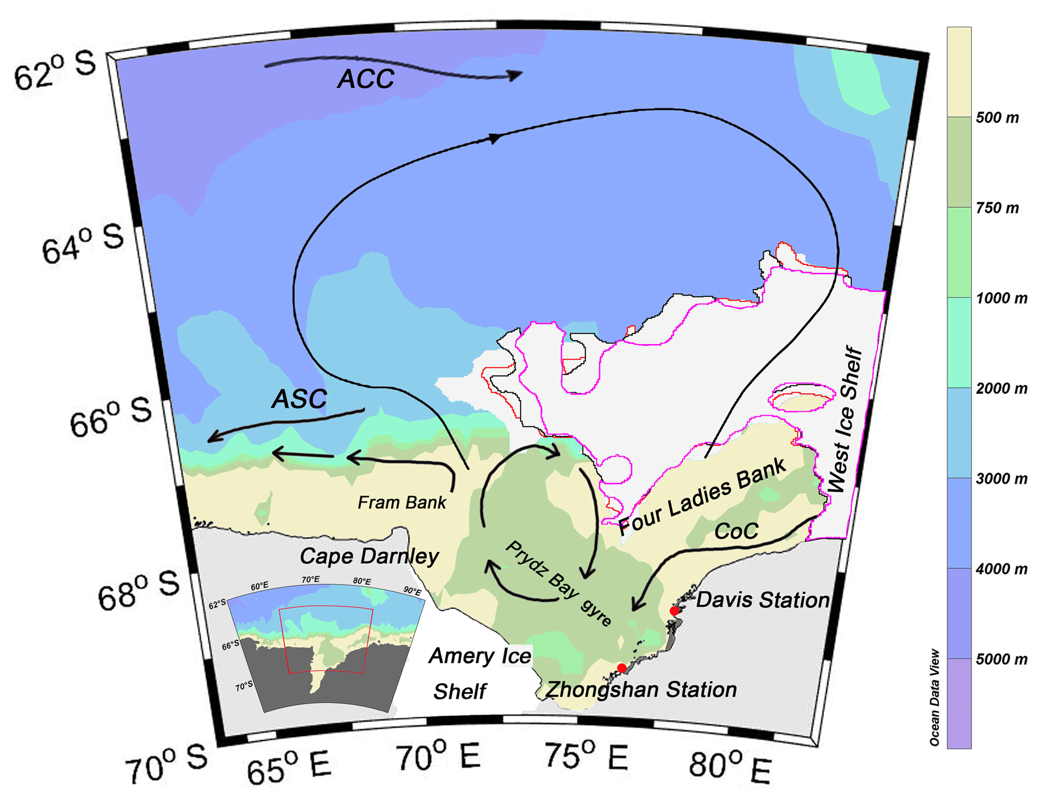
Figure 1 Ocean circulations in Prydz Bay derived from Roden et al. (2013), Sun et al. (2013) and Wu et al. (2017). ASC is the Antarctic Slope Current, CoC is the Antarctic Coastal Current and ACC is the Antarctic Circumpolar Current. During the 4-week cruise, the sea-ice extent varied as indicated by the contoured white areas: the pink line represents week 1 (2–9 February 2015), the black line represents week 2 (10–17 February 2015), the red line represents week 3 (18–25 February 2015) and the unlined white area outside the red contour lines represents week 4 (26 February–5 March 2015).

The inner continental shelf is dominated by the Amery Depression, which generally ranges in depth from 600 to 700 m. This depression is bordered by two shallow banks (< 200 m): the Fram Bank and the Four Ladies Bank, which form a spatial barrier for water exchange with the outer oceanic water (Smith and Trégure, 1994). The Antarctic Coastal Current (CoC) flows westward, bringing in cold waters from the east. When the CoC reaches the shallow Fram Bank, it turns north and then partly flows westward, while some of it turns eastward, back to the inner shelf, resulting in the clockwise-rotating Prydz Bay gyre (see Fig. 1). The circulation to the north of the bay is characterized by a large cyclonic gyre, extending from within the bay to the Antarctic Divergence at approximately 63^∘ S (Nunes Vaz and Lennon, 1996; Middleton and Humphries, 1989; Smith et al., 1984; Roden et al., 2013; Wu et al., 2017). The inflow of this large gyre hugs the eastern rim of the bay and favors the onshore intrusions of the warmer modified Circumpolar Deep Water across the continental shelf break (Heil et al., 1996). Westward flow along the shelf, which is part of the wind-driven Antarctic Slope Current (ASC), supplies water to Prydz Bay.

It has been reported that Prydz Bay is a strong carbon sink, especially in the austral summer (Gibsonab et al., 1999; Gao et al., 2008; Roden et al., 2013). Moreover, studies have shown that the Prydz Bay region is one of the source regions of Antarctic Bottom Water in addition to the Weddell and Ross seas (Jacobs and Georgi, 1977; Yabuki et al., 2006). Thus, it is important to study the carbon cycle in Prydz Bay. However, the analysis of the temporal variability and spatial distribution mechanism of oceanic pCO₂ in the Prydz Bay is limited to cruises or stations due to its unique physical environment and complicated marine ecosystem (Smith et al., 1984; Nunes Vaz et al., 1996; Liu and Cheng, 2003). To estimate regional sea–air CO₂ fluxes, it is necessary to interpolate between in situ measurements to obtain maps of oceanic pCO₂. However, such an interpolation approach is still difficult, as observations are too sparse over both time and space to capture the high variability in pCO₂. Satellites do not measure sea surface pCO₂, but they do provide access to the parameters related to the processes that control its variability. The seasonal and geographical variability of surface water pCO₂ is indeed much greater than that of atmospheric pCO₂. Therefore, the direction of sea–air CO₂ transfer is mainly regulated by oceanic pCO₂, and the method of spatially and temporarily interpolating in situ measurements of oceanic pCO₂ has long been used (Takahashi et al., 2002, 2009; Olsen et al., 2004; Jamet et al., 2007; Chierici et al., 2009). In earlier studies, a linear regression extrapolation method was applied to expand cruise data to study the carbon cycle in the Southern Ocean (Rangama et al., 2005; Chen et al., 2011; Xu et al., 2016). However, this linear regression relied simply on either chlorophyll a (CHL) or sea surface temperature (SST) parameters. Thus, this method can not sufficiently represent all controlling factors. In this study, we applied self-organizing map (SOM) analysis to expand our observed datasets and estimate the oceanic pCO₂ in Prydz Bay from February to early March 2015.

The SOM analysis, which is a type of artificial neural network, has been proven to be a useful method for extracting and classifying features in the geosciences field, such as trends in (and between) input variables (Gibson et al., 2017; Huang et al., 2017b). The SOM uses an unsupervised learning algorithm (i.e., with no need for a priori, empirical or theoretical descriptions of input–output relationships), thus enabling us to identify the relationships between the state variables of the phenomena being analyzed, where our understanding of these cannot be fully described using mathematical equations and where applications of knowledge-based models are consequently limited (Telszewski et al., 2009). In the field of oceanography, SOM has been applied for the analysis of various properties of seawater, such as sea surface temperature (Iskandar, 2010; Liu et al., 2006), and chlorophyll concentration (Huang et al., 2017a; Silulwane et al., 2001). Over the past decade, SOM has also been applied to produce basin-scale pCO₂ maps, mainly in the North Atlantic and Pacific oceans, by using different proxy parameters (Lafevre et al., 2005; Friedrich and Oschlies, 2009a, b; Nakaoka et al., 2013; Telszewski et al., 2009; Hales et al., 2012; Zeng et al., 2015; Laruelle et al., 2017). SOM has been proven to be useful for expanding the spatial–temporal coverage of direct measurements or for estimating properties for which satellite observations are technically limited. One of the main benefits of the neural network method over more traditional techniques is that it provides more accurate representations of highly variable systems of interconnected water properties (Nakaoka et al., 2013).

We conducted a survey during the 31st CHINARE cruise in Prydz Bay (Fig. 2). This study aimed to apply the SOM method, combined with remotely sensed data, to reduce the spatiotemporal scarcity of contemporary pCO₂ data and to obtain a better understanding of the capability of carbon absorption in Prydz Bay from 63 to 83^∘ E and 64 to 70^∘ S from February to early March 2015.

The paper is organized as follows. Section 2 provides descriptions of the in situ measurements and SOM methods. Section 3 presents the analysis and discussion of the results, and Sect. 4 presents a summary of this research.

2 Data and methods

2.1 In situ data

The in situ underway pCO₂ values from marine water and the atmosphere were collected during the 31st CHINARE cruise, when the R/V Xuelong sailed east–west from the beginning of February to early March 2015 (see Fig. 2a, b). Sea water at a depth of 5 m beneath the sea surface was continuously pumped to the GO system (Model 8050 pCO measuring system, General Oceanics Inc., Miami FL, USA), and the partial pressure of the sea surface water was measured using an infrared analyzer (LICOR, USA, Model 7000). The analyzer was calibrated every 2.5–3 h using four standard gases supplied by NOAA's Global Monitoring Division at pressures of 88.82, 188.36, 399.47 and 528.92 ppm. The accuracy of the measured pCO₂ data is within 2 µatm (Pierrot et al., 2009). Underway atmospheric pCO₂ data were simultaneously collected by the GO system. The biological and physical pumps in the ocean (Hardman-Mountford et al., 2009; Bates et al., 1998a, b; Barbini et al., 2003; Sweeney, 2002) are the key factors controlling the variation in sea surface pCO₂. In terms of the physical pumps, the solubility of CO₂ is affected by temperature and salinity, but the biological pumps, such as phytoplankton, take CO₂ up via photosynthesis while organisms release it through respiration (Chen et al., 2011). There are several processes that can influence the distribution of oceanic pCO₂.

Sea-ice melt has a significant impact on the local stratification and circulation in polar regions. During freezing, brine is rejected from ice, thereby increasing the sea surface salinity. When ice begins to melt, fresher water is added into the ocean, thereby diluting the ocean water, i.e., reducing its salinity; thus, changes in salinity record physical processes. In this study, we treat salinity as an index for changes in sea ice. The underway SST and conductivity data were recorded by a conductivity–temperature–depth sensor (CTD, Seabird SBE 21) along the cruise track. Later, sea surface salinity was calculated based on the recorded conductivity and temperature data. The distributions of underway SST and SSS are shown in Fig. 2c and d.

In austral summer, when sea ice started to melt, ice algae were released into the seawater, and the number of living biological species and the amount of primary productivity increased; thus, high chlorophyll a values were observed (Liu et al., 2000; Liu and Cheng, 2003). Previous studies have reported that the summer sink in Prydz Bay is biologically driven and that the change in pCO₂ is often well correlated with the surface chlorophyll a concentration (Rubin et al., 1998; Gibsonab et al., 1999; Chen et al., 2011; Xu et al., 2016). The chlorophyll a value is regarded as an important controlling factor of pCO₂. Remote sensing data of chlorophyll a obtained from MODIS with a resolution of 4 km (http://oceancolor.gsfc.nasa.gov, last access: 14 September 2017) were interpolated according to the cruise track (Fig. 2e).

The ocean mixed layer is characterized as having nearly uniform physical properties throughout the layer, with a gradient in its properties occurring at the bottom of the layer. The mixed layer links the atmosphere to the deep ocean. Previous studies have emphasized the importance of accounting for vertical mixing through the mixed layer depth (MLD; Dandonneau, 1995; Lüger et al., 2004). The stability and stratification of this layer prevent the upward mixing of nutrients and limit biological production, thus affecting the sea–air CO₂ exchange. Two main methods are used to calculate the MLD (Chu and Fan, 2010): one is based on the difference criterion, and one is based on the gradient criterion. Early studies suggested that the MLD values determined in the Southern Ocean using the difference criterion are more stable (Brainerd and Gregg, 1995; Thomson and Fine, 2003). Thus, following Dong et al. (2008), we calculated the MLD (see Fig. 2f) based on the difference criterion, in which σ_θ changed by 0.03 kg m⁻³. The MLD values at the stations along the cruise were later gridded linearly to match the spatial resolution of the underway measurements.

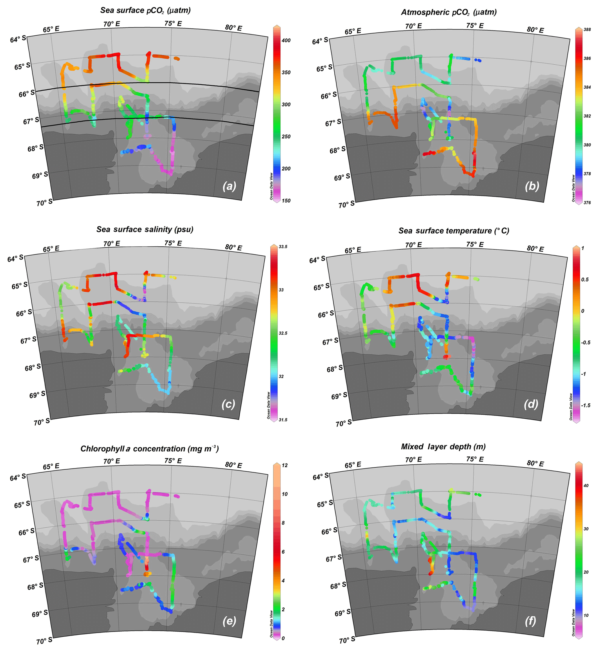
Figure 2 The distributions of underway oceanic and atmospheric pCO₂, SST, SSS and CHL gridded from MODIS, in addition to MLD gridded from station surveys, from February to early March.

2.2 SOM method and input variables

We hypothesize that oceanic pCO₂ can be reconstructed using the SOM method with four proxy parameters (Eq. 1): sea surface temperature (SST), chlorophyll a concentration (CHL), mixed layer depth (MLD) and sea surface salinity (SSS).

$$\begin{array}{}\text{(1)}& p{\mathrm{CO}}_{\mathrm{2}}^{\mathrm{sea}}=\mathrm{SOM}(\mathrm{SST},\mathrm{CHL},\mathrm{MLD},\mathrm{SSS})\end{array}$$

The SOM is trained to project the input space of training samples to a feature space (Kohonen, 1984), which is usually represented by grid points in 2-D space. Each grid point, which is also called a neuron cell, is associated with a weight vector that has the same number of components as the vector of the input data (Zeng et al., 2017). During SOM analysis, three steps are taken following Nakaoka et al. (2013) to estimate the oceanic pCO₂ fields (see Fig. 3). As the four input environmental parameters (SST, CHL, MLD and SSS) are used to estimate pCO₂ in this study, each input dataset is prepared in 4-D vector form. Here, the SOM analysis was carried out using the MATLAB SOM tool box 2.0 (Vesanto, 2002). This toolbox was developed by the Laboratory of Computer and Information Science at the Helsinki University of Technology and is available from the following web page: http://www.cis.hut.fi/projects/somtoolbox (last access: June 2016).

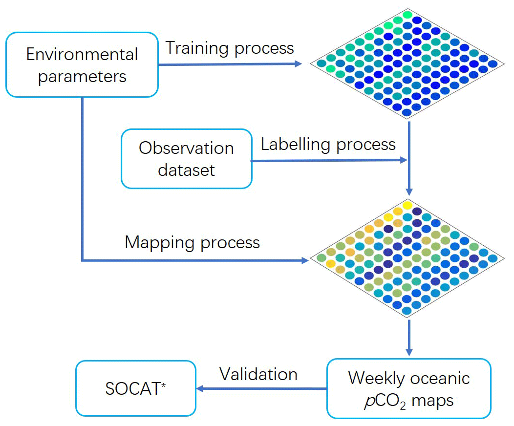
Figure 3 Schematic diagram of the main three steps involved in the SOM neural network calculations used to obtain weekly pCO₂ maps for February to early March 2015.

During the training process, each neuron's weight vectors (P_i), which are linearly initialized, are repeatedly trained by being presented with the input vectors (Q_j) of environmental parameters in the SOM training function. Because SOM analysis is known to be a powerful technique with which to estimate pCO₂ based on the nonlinear relationships of the parameters (Telszewski et al., 2009), we assumed that the nonlinear relationships of the proxy parameters are sufficiently represented after the training procedure. During this step, Euclidean distances (D) are calculated between the weight vectors of neurons and the input vectors as shown in Eq. (2), and the neuron with the shortest distance is selected as the winner. This process results in the clustering of similar neurons and the self-organization of the map. The observed oceanic pCO₂ data are not needed in the first step.

$$\begin{array}{ll}\text{(2)}& {\displaystyle }& {\displaystyle }D({\mathit{P}}_i,{\mathit{Q}}_j){\displaystyle }& {\displaystyle }=\sqrt{\left\{\begin{array}{c}{\left(P_{i\mathit{\_}\mathrm{SST}}-Q_{j\mathit{\_}\mathrm{SST}}\right)}^{\mathrm{2}}+{\left(P_{i\mathit{\_}\mathrm{CHL}}-Q_{j\mathit{\_}\mathrm{CHL}}\right)}^{\mathrm{2}}\\ +{\left(P_{i\mathit{\_}\mathrm{MLD}}-Q_{j\mathit{\_}\mathrm{MLD}}\right)}^{\mathrm{2}}+{\left(P_{i\mathit{\_}\mathrm{SSS}}-Q_{j\mathit{\_}\mathrm{SSS}}\right)}^{\mathrm{2}}\end{array}\right\}}\end{array}$$

During the second part of the process, each preconditioned SOM neuron is labelled with an observation dataset of in situ oceanic pCO₂values, and the labelling process technically follows the same principles as the training process. The labelling dataset, which consists of the observed pCO₂ and normalized SST, CHL, MLD and SSS data, is presented to the neural network. We calculated the D values between trained neurons and observational environmental datasets. The winner neuron is selected as in step 1 and labelled with an observed pCO₂ value. After the labelling process, the neurons are represented as 5-D vectors.

Finally, during the mapping process, the labelled SOM neurons created by the second process and the trained SOM neurons created by the first process are used to produce the oceanic pCO₂ value of each winner neuron based on its geographical grid point in the study area.

Before the training process, the input training dataset and labelling dataset are analyzed and prospectively normalized to create an even distribution. The statistics and ranges of the values of all variables are presented in Table 1. When the datasets of the four proxy parameters were logarithmically normalized, the skewness values of CHL and MLD changed, especially for the training dataset. The N coverage represents the percentage of the training data that are labelled. The data N coverage values of the training datasets of CHL, MLD and SSS are 82.1 %, 85 % and 81.1 %, respectively, which may be due to their insufficient spatiotemporal coverage and/or bias between the labelling and training datasets. The N coverage of the logarithmic datasets changed to 93.6 % and 98.7 % for CHL and MLD, respectively. Thus, the common logarithms of the CHL and MLD values are used for both the training and labelling datasets to resolve the data coverage issue arising from significantly increasing the data coverage as well as to overcome the weighting issue arising from the different magnitudes between variables (Ultsch and Röske, 2002).

Table 1 Statistics of labelling and training datasets showing the distribution and coverage of each variable.

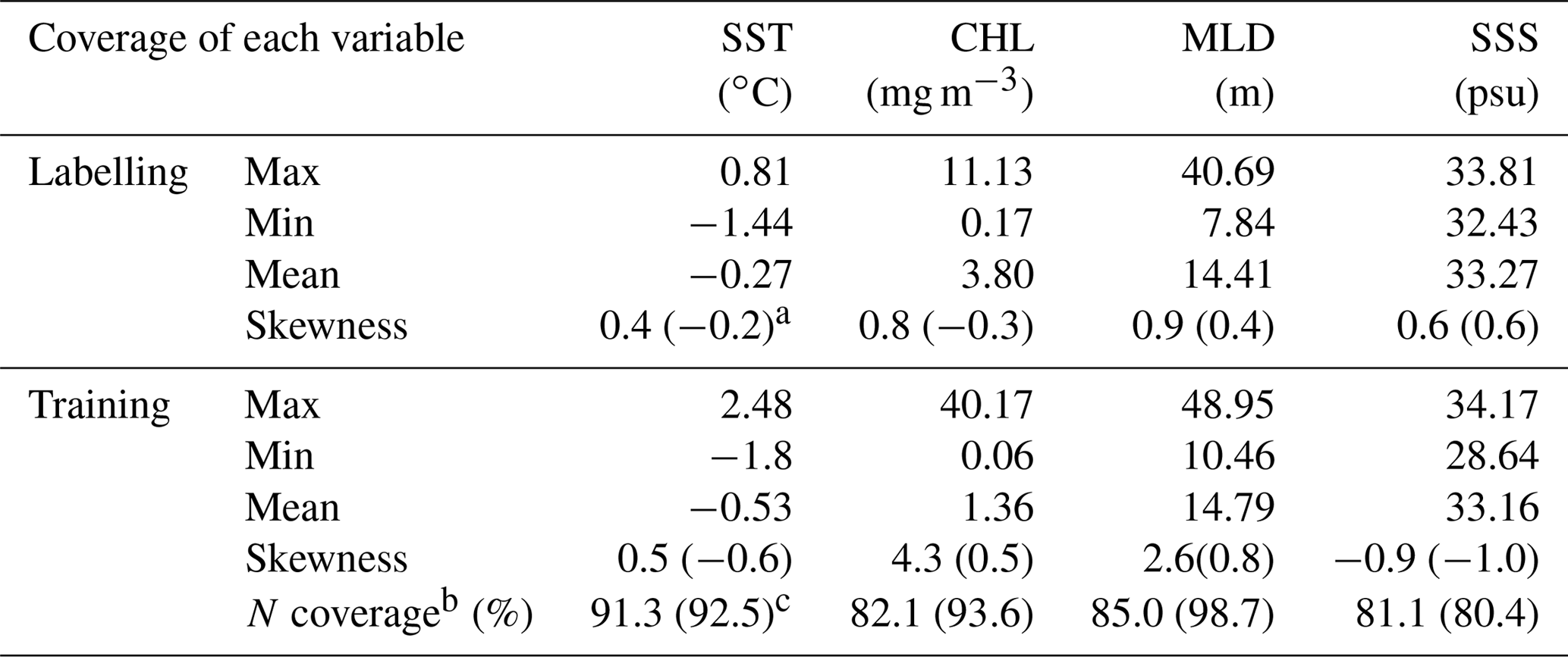
^a The skewness of the common logarithm of each variable is shown in parentheses. ^b Number of training data within the labelling data range/total number of training data. ^c The percent labelling data coverage of normalized variables is shown in parentheses.

In this study, we construct weekly oceanic pCO₂ maps from February to early March 2015 using four datasets, i.e., SST, CHL, MLD and SSS. Considering the size of our study region, we chose a spatial resolution of 0.1^∘ latitude by 0.1^∘ longitude. For SST, we used daily data from AVHRR-Only (https://www.ncdc.noaa.gov/oisst, last access: 22 September 2017) with a $\mathrm{1}/\mathrm{4}{}^{\circ }$ spatial resolution (see Fig. S1 in the Supplement). The CHL data represent the 8-day composite chlorophyll a data from MODIS-Aqua (http://oceancolor.gsfc.nasa.gov, last access: 14 September 2017) with a spatial resolution of 4 km (see Fig. S2). We also used the daily SSS and MLD data (see Figs. S3–S4) from the $\mathrm{1}/\mathrm{12}{}^{\circ }$ global analysis and forecast product from the Copernicus Marine Environment Monitoring Service (CMEMS, http://marine.copernicus.eu/, last access: 28 September 2017). Sea-ice concentration data are from the daily 3.125 km AMSR2 dataset (Spreen et al., 2008, available on https://seaice.uni-bremen.de, last access: 30 September 2017, see Fig. S5).

All daily datasets were first averaged to 8-day fields, which are regarded as weekly in this study. The period from the beginning of February to early March comprises four independent weeklong series: week 1 (2–9 February 2015), week 2 (10–17 February 2015), week 3 (18–25 February 2015) and week 4 (26 February–5 March 2015). The weekly proxy parameters (SCMS) were further re-gridded to a horizontal resolution of $\mathrm{0.1}{}^{\circ }\times \mathrm{0.1}{}^{\circ }$ using the kriging method in Surfer software (version 7.3.0.35). In the SOM analyses, input vectors with missing elements are excluded. We compared the assimilated datasets of SST from AVHRR with the in situ measurements obtained by CTD along the cruise. Their correlation is 0.97, and their root mean square error (RMSE) is 0.2 ^∘C. Comparing the SSS and MLD fields from the Global Forecast System with the in situ measurements yields correlations of 0.76 and 0.74 and RMSEs of 0.41 psu and 5.15 m, respectively. The uncertainty of the MODIS CHL data in the Southern Ocean is approximately 35 % (Xu et al., 2016). For the labelling procedure, the observed oceanic pCO₂ and the corresponding in situ SST, SSS, MLD and MODIS CHL products in vector form are used as the input dataset.

2.3 Validation of SOM-derived oceanic pCO₂

More realistic pCO₂ estimates are expected from SOM analyses when the distribution and variation ranges of the labelling variables closely reflect those of the training datasets (Nakaoka et al., 2013). However, our underway measurements of pCO₂ values have spatiotemporal limitations preventing them from covering the range of variation of the training datasets. To validate the oceanic pCO₂ values reconstructed by the SOM analysis, we used the fugacity of oceanic CO₂ datasets from the Surface Ocean CO₂ Atlas (hereafter referred to as “SOCAT” data, http://www.socat.info, last access: 14 November 2017) version 5 database (Bakker et al., 2016). We selected the dataset from SOCAT (the EXPOCODE is 09AR20150128, see cruise in Fig. 4a) that coincided with the same period as our study. The cruise lasted from 6 to 27 February 2015, and fCO₂ measurements were made every 1 min at a resolution of 0.01^∘. We recalculated pCO₂ values based on the fCO₂ values provided by the SOCAT data using the fugacity correction (Pfeil et al., 2013).

2.4 Carbon uptake in Prydz Bay

The flux of CO₂ between the atmosphere and the ocean was determined using ΔpCO₂ and the transfer velocity across the sea–air interface, as shown in Eq. (3), where K is the gas transfer velocity (in cm h⁻¹), and the quadratic relationship between wind speed (in units of m s⁻¹) and the Schmidt number is expressed as $(\mathit{\text{Sc}}/\mathrm{660}{)}^{-\mathrm{0.5}}$. L is the solubility of CO₂ in seawater (in mol L⁻¹ atm⁻¹) (Weiss, 1974). For the weekly estimation in this study, the scaling factor for the gas transfer rate is changed to 0.251 for shorter timescales and intermediate wind speed ranges (Wanninkhof, 2014). Considering the unit conversion factor (Takahashi et al., 2009), the weekly sea–air carbon flux in Prydz Bay can be estimated using Eq. (4):

$$\begin{array}{ll}\text{(3)}& {\displaystyle }& {\displaystyle }{\mathrm{Flux}}_{\text{sea-air}}=K\times L\times \mathrm{\Delta }p{\mathrm{CO}}_{\mathrm{2}}\text{(4)}& {\displaystyle }& {\displaystyle }{\mathrm{Flux}}_{\text{sea-air}}[\mathrm{gC}/({\mathrm{m}}^{\mathrm{2}}\mathrm{week}\left)\right]{\displaystyle }& {\displaystyle }=\mathrm{30.8}\times {\mathrm{10}}^{-\mathrm{4}}\times U^{\mathrm{2}}\times \left(p{\mathrm{CO}}_{\mathrm{2}}^{\mathrm{sea}}-p{\mathrm{CO}}_{\mathrm{2}}^{\mathrm{air}}\right),\end{array}$$

where U represents the wind speed 10 m a.s.l., and $p{\mathrm{CO}}_{\mathrm{2}}^{\mathrm{sea}}$ and $p{\mathrm{CO}}_{\mathrm{2}}^{\mathrm{air}}$ are the partial pressures of CO₂ in sea water and the atmosphere, respectively.

We downloaded weekly ASCAT wind speed data (http://www.remss.com/, last access: 25 September 2017, see Fig. S6) with a resolution of $\mathrm{1}/\mathrm{4}{}^{\circ }$ and then gridded the dataset to fit the 0.1^∘ longitude × 0.1^∘ latitude spatial resolution of the SOM-derived oceanic pCO₂. We gridded the atmospheric pCO₂ data collected along the cruise track to fit the spatial resolution of the SOM-derived oceanic pCO₂ data using a linear method. The total carbon uptake was then obtained by accumulating the flux of each grid in each area according to Jiang et al. (2008) and using the proportion of ice-free areas (Takahashi et al., 2012). When the ice concentration is less than 10 % in a grid, we regard the grid box as comprising all water. When the ice concentration falls between 10 % and 90 %, the flux is computed as being proportional to the water area. In the cases of leads or polynyas due to the dynamic motion of sea ice (Worby et al., 2008), we assume the grid box to be 10 % open water when the satellite sea-ice cover is greater than 90 %.

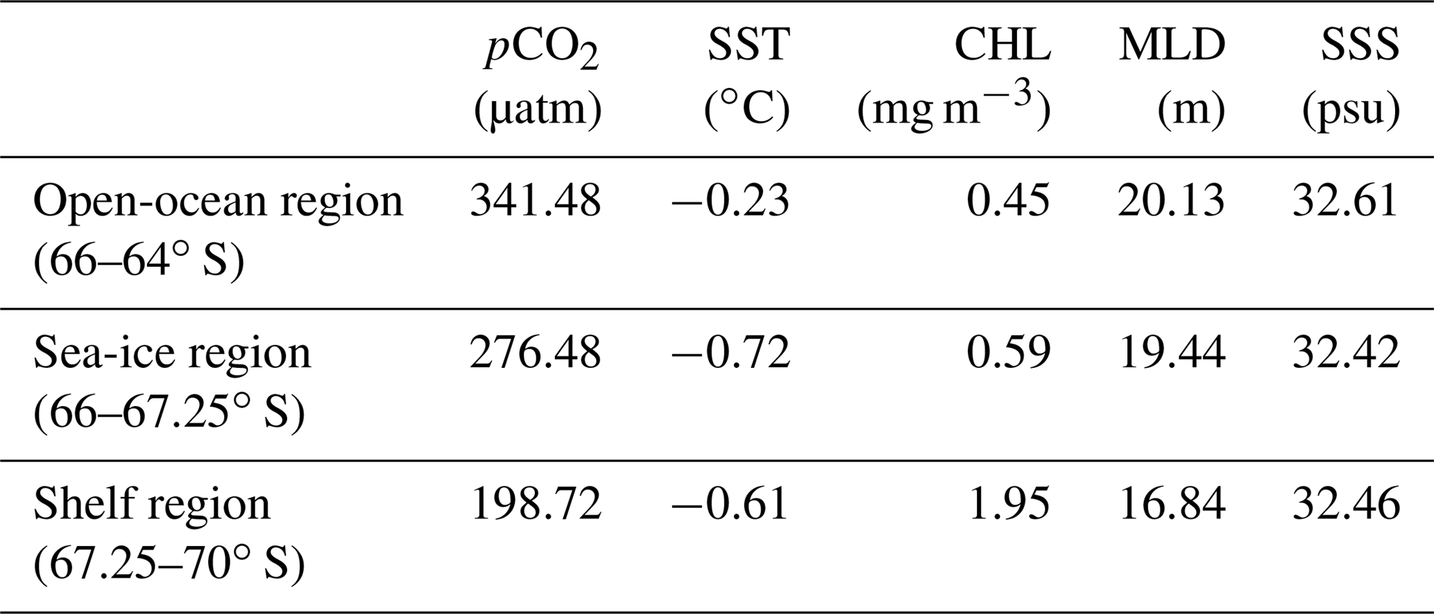
Table 2 The regional mean values of underway measurements in three subregions.

3 Results and discussion

3.1 The distributions of underway measurements

During austral summer, daylight lasts longer and solar radiation increases. With increasing sea surface temperature, ice shelves break and sea-ice melts, resulting in the stratification of the water column. Starting at the beginning of February, the R/V Xuelong sailed from east to west along the sea-ice edge, and its underway measurements are shown in Fig. 2. Based on the water depth and especially the different ranges of oceanic pCO₂ (see Fig. 2a; Table 2), the study area can be roughly divided into three regions, namely, the open-ocean region, the sea-ice region and the shelf region (see Table 2).

The open-ocean region ranges northward from 66 to 64^∘ S, where the Antarctic Divergence Zone is located and water depths are greater than 3000 m. In the open-ocean region, the oceanic pCO₂ was the highest, varying from 291.98 to 379.31 µatm, with a regional mean value of 341.48 µatm. The Antarctic Divergence Zone was characterized by high nutrient concentrations and low chlorophyll concentrations, with high pCO₂ attributed to the upwelling of deep waters, thus suggesting the importance of physical processes in this area (Burkill et al., 1995; Edwards et al., 2004). The underway sea surface temperatures in this region are relatively high, with an average value of −0.23 ^∘C due to the upwelling of Circumpolar Deep Water (CDW), while at the sea-ice edge (73^∘ E, 65.5^∘ S to 72^∘ E, 65.8^∘ S), the SST decreased to less than −1 ^∘C. From 67.5^∘ E westward, affected by the large gyre, cold water from high latitudes lowered the SST to less than 0 ^∘C. Near the sea-ice edge, SSS decreased quickly to 31.7 psu due to the diluted water; along the 65^∘ S cruise, it reached 33.3 psu; then, moving westward from 67.5^∘ E, affected by the fresher and colder water brought by the large gyre, it decreased to 32.5 psu. The satellite chlorophyll a image showed that the regional mean was as low as 0.45 mg m⁻³, except when the vessel near the sea-ice edge recorded CHL values that increased to 2.26 mg m⁻³. The lowest pCO₂ value was found near the sea-ice edge due to biological uptake. The distribution of MLD varied along the cruise. Near the sea-ice edge, because of the melting of ice and direct solar warming, a low-density cap existed over the water column, and the MLD was as shallow as 10.21 m. The maximum value of the MLD in the open-ocean region was 31.67 m. In this domain, atmospheric pCO₂ varied from 374.6 to 387.8 µatm. Along the 65^∘ E cruise in the eastern part of the open-ocean region, the oceanic pCO₂ was relatively high, reaching equilibrium with atmospheric pCO₂. In the western part of this region, the oceanic pCO₂ decreased slightly due to the mixture of low pCO₂ from higher latitudes brought by the large gyre. Mixing and upwelling were the dominant factors affecting the oceanic pCO₂ in this domain.

The seasonal sea-ice region (from 66 to 67.25^∘ S) is located between the open-ocean region and the shelf region. In this sector, sea ice changed strongly, and the water depth varied sharply from 700 to 2000 m. The oceanic pCO₂ values ranged from 190.46 to 364.43 µatm, with a regional mean value of 276.48 µatm. Sea ice continued to change and reform from late February to the beginning of March (Fig. 6). The regional mean sea surface temperature decreased slightly compared to that in the open-ocean region, and the average value was −0.72 ^∘C. With the rapid changes in sea ice, the sea surface temperature and salinity varied sharply from −1.3 to 0.5 ^∘C and from 31.8 to 33.3 psu, respectively. When sea ice melted, the water temperature increased, biological activity increased and the chlorophyll a value increased slightly to reach a regional average of 0.59 mg m⁻³. Due to the rapid change in sea-ice cover, the value of MLD varied from 12.8 to 30.9 m.

The shelf region (from 67.25^∘ S southward) is characterized by shallow depths of less than 700 m, and it is surrounded by the Amery Ice Shelf and the West Ice Shelf. Water inside the shelf region is formed by the modification of low-temperature and high-salinity shelf water (Smith et al., 1984). The Prydz Bay coastal current flows from east to west in the semi-closed bay. The oceanic pCO₂ values in this region were the lowest of those in all three sectors; these values ranged from 151.70 to 277.78 µatm, with a regional average of 198.72 µatm. A fresher, warmer surface layer is always present over the bay, which is known as the Antarctic Surface Water (ASW). During our study period, the shelf region was the least ice-covered region. A large volume of freshwater was released into the bay, resulting in a low sea surface temperature (an average of −0.61 ^∘C) and salinity (an average of 32.4 psu) values. As shown in Fig. 2f, the MLD in most of the inner shelf is low. Due to the vast shrinking of sea ice and strong stratification in the upper water, algal blooming occurred and chlorophyll values were high, with an average value of 1.93 mg m⁻³. The chlorophyll a value was remarkably high, reaching 11.04 mg m⁻³ when sea ice retreated in an eastward direction from 72.3^∘ E, 67.3^∘ S to 72.7^∘ E, 68^∘ S. The biological pump became the dominant factor controlling the distribution of oceanic pCO₂. In the bay mouth close to the Fram Bank, due to local upwelling, the water salinity increased remarkably to approximately 33.2 psu.

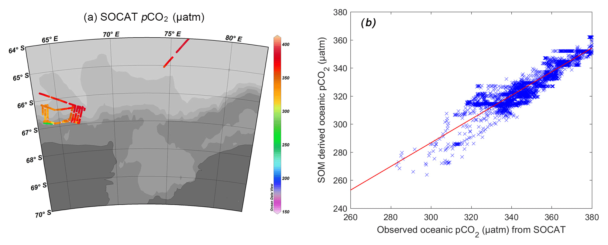
Figure 4 (a) The cruise lines from SOCAT used to validate the SOM-derived oceanic pCO₂ for the study period in 2015; (b) the comparison between the SOM-derived and observed SOCAT oceanic pCO₂ data.

3.2 Quality and maps of SOM-derived oceanic pCO₂

We selected SOM-derived oceanic pCO₂ values to fit the cruise track of SOCAT for the same period in February 2015 using a nearest-grid method. The RMSE between the SOCAT data and the SOM-derived result was calculated as follows:

$$\begin{array}{}\text{(5)}& \mathrm{RMSE}=\sqrt{{\displaystyle \frac{\sum {\left(p{\mathrm{CO}}_{\mathrm{2}}^{\mathrm{sea}}\left(\mathrm{SOM}\right)-p{\mathrm{CO}}_{\mathrm{2}}^{\mathrm{sea}}\left(\mathrm{SOCAT}\right)\right)}^{\mathrm{2}}}{n}}},\end{array}$$

where n is the number of validation datasets. The RMSE can be interpreted as an estimation of the uncertainty in the SOM-derived oceanic pCO₂ in Prydz Bay. In this study, the RMSE of the SOM-derived oceanic pCO₂ and SOCAT datasets is 22.14 µatm, and the correlation coefficient R² is 0.82. The absolute mean difference is 23.58 µatm. The RMSE obtained in our study is consistent with the accuracies (6.9 to 24.9 µatm) obtained in previous studies that used neuron methods to reconstruct oceanic pCO₂ (Nakaoka et al., 2013; Zeng et al., 2002; Sarma et al., 2006; Jo et al., 2012; Hales et al., 2012; Telszewshi et al., 2009). The precision of this study is on the high side of those that have been previously reported. The slope of the scatterplot indicates that the SOM-derived oceanic pCO₂ data are lower than the SOCAT data (see Fig. 4b). Thus, the precision of these data may have greater uncertainty because the SOCAT dataset does not cover the low-pCO₂ area towards the south. Hence, increasing the spatial coverage of the labelling data will help increase the precision of the SOM-derived oceanic pCO₂.

3.3 Spatial and temporal distributions of SOM-derived oceanic pCO₂

The weekly mean maps of SOM-derived oceanic pCO₂ in Prydz Bay are shown in Fig. 5. In the open-ocean region, the oceanic pCO₂ values were higher than those in the other two regions due to the upwelling of the CDW. During all 4 weeks, this region was nearly ice-free, while the average sea-ice coverage was 18.14 % due to the presence of permanent sea ice (see Fig. 6). The oceanic pCO₂ distribution decreased from east to west in the open-ocean region, with lower values observed at the edge of sea ice. In the western part of the open-ocean region, oceanic pCO₂ decreased due to mixing with low oceanic pCO₂ flowing from high-latitude regions caused by the large gyre. From week 1 to week 4, the maximum oceanic pCO₂ increased slightly and reached 381.42 µatm, which was equivalent to the pCO₂ value of the atmosphere.

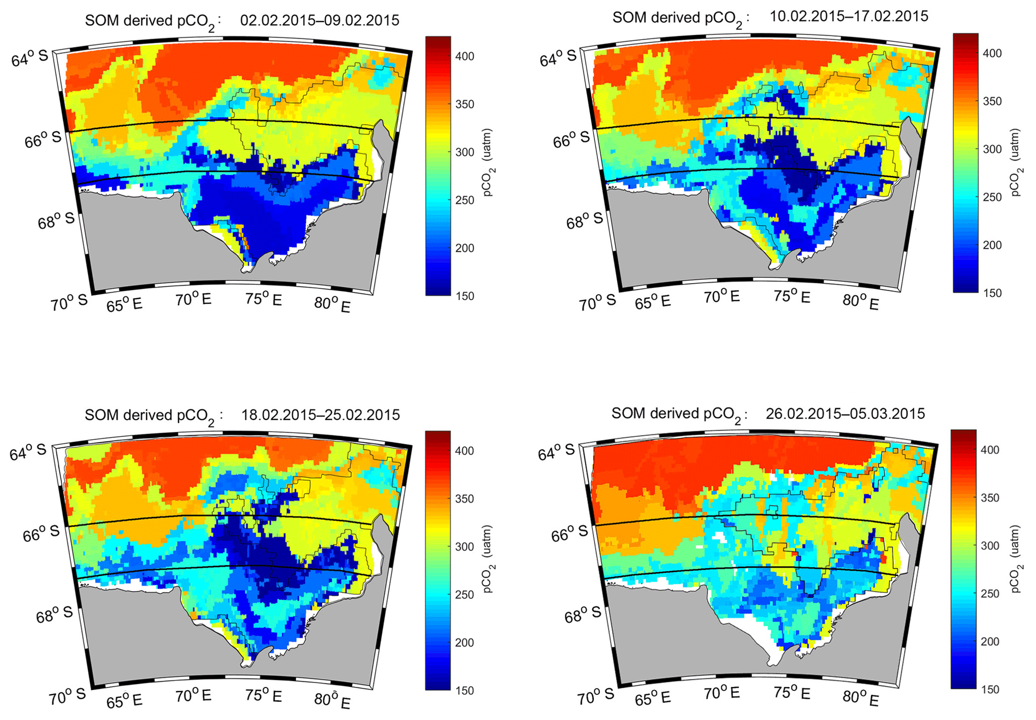
Figure 5 Distribution of weekly mean SOM-derived oceanicpCO₂ in Prydz Bay (in µatm) from 2 February to 5 March 2015. The black contour represents a sea-ice concentration of 15 %.

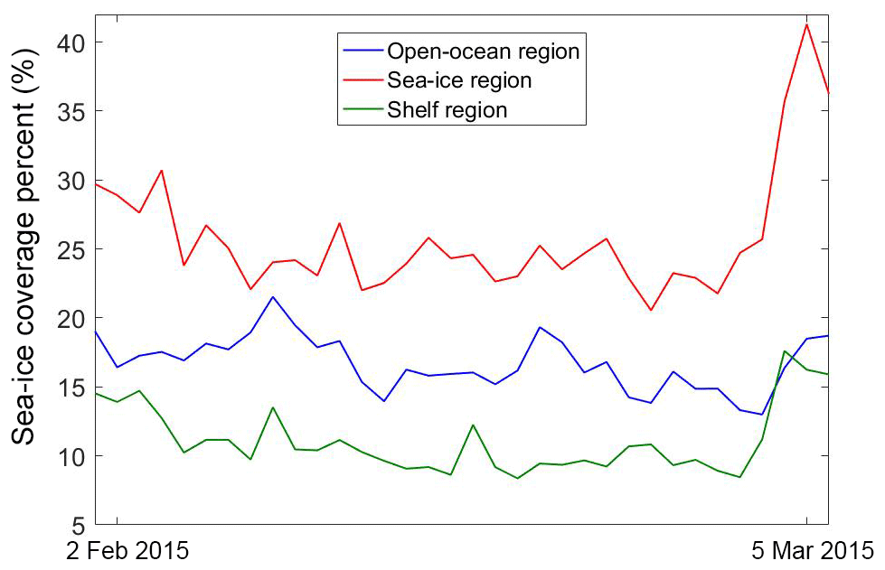
Figure 6 Percentage of sea-ice coverage in three subregions from 2 February to 5 March 2015 (blue represents the open-ocean region, red represents the sea-ice region and green represents the shelf region).

In the sea-ice region, sea ice continued to rapidly melt and reform. The weekly mean sea-ice coverage percentage was 29.54 %, occupying nearly one-third of the sea-ice region. As shown in Fig. 5, the gradient of the oceanic pCO₂ distribution increased from south to north affected by the flow coming from the shelf region due to the large gyre. In the eastern part of this region, adjacent to the sea-ice edge, the oceanic pCO₂ values were lower. The oceanic pCO₂ changed sharply from 155.86 µatm (near the sea-ice edge) to 365.11 µatm (close to the open-ocean region).

In austral winter, the entire Prydz Bay basin is fully covered by sea ice, except in a few areas, i.e., the polynyas, which remain open owing to katabatic winds (Liu et al., 2017). When the austral summer starts, due to coincident high wind speeds, monthly peak tides, and/or the effect of penetrating ocean swells, the sea ice in the shelf region starts to melt first (Lei et al., 2010), forming the Prydz Bay polynya. The semi-closed polynya functions as a barrier for water exchange in the shelf region and causes a lack of significant bottom water production, hindering the outflow of continental shelf water and the inflow of Antarctic circle deep water, resulting in the longer residence time of vast melting water and enhanced stratification (Sun et al., 2013). Due to vast melting of the sea ice, the sea surface salinity decreased and algae bloomed; biological productivity promptly increased, and the chlorophyll a concentration reached its peak value. As shown in Fig. 5, the distribution of oceanic pCO₂ in the shelf region was characterized by its lowest values. The obvious drawdown of oceanic pCO₂ occurred in the shelf region due to phytoplankton photosynthesis during this summer bloom. The lowest oceanic pCO₂ in the shelf region was 153.83 µatm, except at the edge of the West Ice Shelf, where the shelf oceanic pCO₂ exceeded 300 µatm. The oceanic pCO₂ was the lowest in week 1, which coincided with a peak in chlorophyll a, as evidenced by satellite images. The regional oceanic pCO₂ increased slightly in week 4 compared to the other 3 weeks.

Table 3 Regional and weekly mean ΔpCO₂, wind speed and uptake of CO₂ in three subregions (negative values represent directions moving from air to sea).

3.4 Carbon uptake in Prydz Bay

During our study period, the entire region was undersaturated, with CO₂ being absorbed by the ocean. The regional averaged ocean–air pCO₂ difference (ΔpCO₂) was highest in the shelf region, followed by the sea-ice region and the open-ocean region (see Table 3). The regional and weekly mean ΔpCO₂ in the shelf region changed from −184.31 µatm in week 1 to −141.00 µatm in week 2 as chlorophyll decreased. The ΔpCO₂ in the sea-ice region and open-ocean region showed the same patterns, increasing from week 1 to week 3 and then decreasing in week 4. Based on the ΔpCO₂ and wind speed data, the uptake of CO₂ in these three regions is presented in Table 3. The uncertainty of the carbon uptake depends on the errors associated with the wind speed, the scaling factor and the accuracy of the SOM-derived pCO₂ according to Eq. (4). The scaling factor will yield a 20 % uncertainty in the regional flux estimation. The errors in the wind speeds of the ASCAT dataset are assumed to be 6 % (Xu et al., 2016); the error in the quadratic wind speed is 12 %.The RMSE of the SOM-derived pCO₂ is 22.14 µatm. Considering the errors described above and the uncertainty occurring when the sea–air computation expression is simplified (1.39 %, Xu et al., 2016), the total uncertainty of the final uptake is 27 %. In the shelf region, the low oceanic pCO₂ levels drove relatively intensive CO₂ uptake from the atmosphere. The carbon uptake in the shelf region changed from week 1 (2.51±0.68 TgC, 10¹² g Tg) to week 2 (2.77±0.75 TgC). In contrast, in week 3, the wind speed slowed down, resulting in the uptake of CO₂ in the shelf region decreasing to 2.10±0.57 TgC. In week 4, even though the ΔpCO₂ was the lowest of all 4 weeks, the total absorption still increased to 2.63±0.715 TgC due to the high wind speed (with an average value of 7.92 m s⁻¹). The total carbon uptake in the three regions of Prydz Bay, integrated from February to early March 2015, was 23.57 TgC, with an uncertainty of ±6.36 TgC.

Roden et al. (2013) estimated coastal Prydz Bay to be an annual net sink for CO₂ of 0.54±0.11 mol m⁻² year⁻¹, i.e., 1.48±0.3 g m⁻² week⁻¹. Gibsonab et al. (1999) estimated the average sea–air flux in the summer ice-free period to be more than 30 mmol m⁻² day⁻¹, i.e., 9.2 g m⁻² week⁻¹. Our study suggests that the sea–air flux during the strongest period of the year, i.e., February, could be much larger. The average flux obtained here, 18.84 g m⁻² week⁻¹, is twice as large as the average value estimated over a longer period (November to February) reported by Gibsonab et al. (1999).

As the region recording the strongest surface unsaturation of these three regions in summer, the shelf region has a potential carbon uptake of 10.01±2.7 TgC from February to early March, which accounts for approximately 5.0 ‰–6.7 ‰ of the net global ocean CO₂ uptake according to Takahashi et al. (2009), even though its total area is only 78×10³ km². Due to the sill constraint, there is limited exchange between water masses in and outside Prydz Bay. During winter, the dense water formed by the ejection of brine in the bay can potentially uptake more anthropogenic CO₂ from the atmosphere that can descend to greater depths, thus enhancing the acidification in deep water. According to Shadwick et al. (2013), the winter pH and Ω values decrease more remarkably than those in summer. As the bottom water in Prydz Bay is a possible source of Antarctic Bottom Water (Yabuki et al., 2006), the shelf region may transfer anthropogenic CO₂ at the surface to deep water; thus, this region may influence the acidification of the deep ocean over long timescales.

4 Summary

Based on the different observed ranges of the distribution of ocean pCO₂, the Prydz Bay region was divided into three sectors from February to early March 2015. In the shelf region, biological factors exerted the main control on oceanic pCO₂, while in the open-ocean region, mixing and upwelling were the main controls. In the sea-ice region, due to rapid changes in sea ice, oceanic pCO₂ was controlled by both biological and physical processes. SOM is an important tool for the quantitative assessment of oceanic pCO₂ and its subsequent sea–air carbon flux, especially in dynamic, high-latitude, and seasonally ice-covered regions. The estimated results revealed that the SOM technique can be used to reconstruct the variations in oceanic pCO₂ associated with biogeochemical processes expressed by the variability in four proxy parameters: SST, CHL, MLD and SSS. The RMSE of the SOM-derived oceanic pCO₂ is 22.14 µatm for the SOCAT dataset. From February to early March 2015, the Prydz Bay region was a strong carbon sink, with a carbon uptake of 23.57±6.36 TgC. The strong potential uptake of anthropogenic CO₂ in the shelf region will enhance the acidification in the deep-water region of Prydz Bay and may thus influence the acidification of the deep ocean in the long run because it contributes to the formation of Antarctic Bottom Water.