Validation of demographic equilibrium theory against tree-size distributions and biomass density in Amazonia

Predicting the response of forests to climate and land-use change depends on models that can simulate the time-varying distribution of different tree sizes within a forest – so-called forest demography models. A necessary condition for such models to be trustworthy is that they can reproduce the tree-size distributions that are observed within existing forests worldwide. In a previous study, we showed that demographic equilibrium theory (DET) is able to fit tree-diameter distributions for forests across North America, using a single site-specific fitting parameter (μ) which represents the ratio of the rate of mortality to growth for a tree of a reference size. We use a form of DET that assumes tree-size profiles are in a steady state resulting from the balance between a size-independent rate of tree mortality and tree growth rates that vary as a power law of tree size (as measured by either trunk diameter or biomass). In this study, we test DET against ForestPlots data for 124 sites across Amazonia, fitting, using maximum likelihood estimation, to both directly measured trunk diameter data and also biomass estimates derived from published allometric relationships. Again, we find that DET fits the observed tree-size distributions well, with best-fit values of the exponent relating growth rate to tree mass giving a mean of ϕ=0.71 (0.31 for trunk diameter). This finding is broadly consistent with exponents of ϕ=0.75 ($\mathit{\varphi }=\mathrm{1}/\mathrm{3}$ for trunk diameter) predicted by metabolic scaling theory (MST) allometry. The fitted ϕ and μ parameters also show a clear relationship that is suggestive of life-history trade-offs. When we fix to the MST value of ϕ=0.75, we find that best-fit values of μ cluster around 0.25 for trunk diameter, which is similar to the best-fit value we found for North America of 0.22. This suggests an as yet unexplained preferred ratio of mortality to growth across forests of very different types and locations.

1 Introduction

The modelling of the abundances of various tree sizes in tropical forests is important in efforts to improve understanding of land–climate feedbacks and hence anthropogenic climate change. Earth system models (ESMs) are used to model climate but currently have a large range of uncertainty in the prediction of the land carbon sink, with as much as 500 GtC uncertainty by 2100 for a 1 % increase in CO₂ emissions per year (Friedlingstein et al., 2014). This uncertainty feeds through into estimates of how much emissions need to be reduced to keep global warming within a certain level. These issues have led to the development of more advanced dynamic global vegetation models (DGVMs), used within ESMs, to more effectively represent vegetation processes (Sitch et al., 2015; Fisher et al., 2018). One of the key advances has been the inclusion of tree-size distributions, which allows for the better representation of land-use change and recovery from disturbance.

These recent DGVMs broadly consist of two different approaches to representing tree size, either based on individual-based models (Shugart et al., 2018) or using cohort-based ecosystem demography models (Moorcroft et al., 2001; Longo et al., 2019). DGVMs also need to balance additional complexity against practical considerations of usability, as well as computer execution time and memory usage. Key issues in the usability of complex numerical models are the understanding of the effect of many model parameters and the dependence on initial conditions (Moore et al., 2018). To solve these issues we have been exploring simplifications to the modelling of forest demography that are parameter sparse and have steady-state solutions that can be solved for analytically (Moore et al., 2018; Argles et al., 2019).

We follow demographic equilibrium theory (DET) (Muller-Landau et al., 2006b) in assuming that forests are in a steady state with size distributions completely determined by size-dependent functions of tree growth and mortality. Previously we showed that DET was able to fit the large-scale size distributions of forests in North America (Moore et al., 2018), even though many of these forests are net carbon sinks (and therefore not in a precise steady state). The current study uses the simplest reasonable form of DET that assumes growth is a power law of size and mortality is constant. This form of DET has been shown to be a useful model of underlying demographic processes, with the model parameters correlating with observations (Muller-Landau et al., 2006b; Lima et al., 2016), even though individual forest plots may deviate from the simplifying assumptions. While the growth and mortality functions of a forest are often unknown, DET can provide useful indications of the patterns of the ratio of mortality to growth based on observed tree-size distributions alone (Moore et al., 2018).

Amazonia is one of the largest pools of land carbon on the planet (Feldpausch et al., 2012) and may be vulnerable to climate change (Cox et al., 2000; Brienen et al., 2015). It is therefore vital that DGVMs are able to model this region well. We therefore extend the analysis of Moore et al. (2018) by fitting the DET model to tree trunk diameter data for this key region, and also to tree mass data derived from allometry, which is even more relevant for ESMs. As a baseline comparison we also fit the metabolic scaling theory of forest demography (MSTF), which assumes that trees of varying sizes fill space in such a way that the size-distribution scales with trunk diameter D as D⁻² (West et al., 2009).

In Sect. 2 below we summarise the theoretical basis for DET and also MSTF, deriving analytical formulae for total forest biomass in each case. Section 3 describes the methods and data, and Sect. 4 describes the results. Finally discussion and conclusions are in Sects. 5 and 6.

2 Theory

2.1 Demographic equilibrium theory (DET)

The distribution of tree sizes in a forest can be understood in terms of how the growth and mortality of the trees vary with tree size (Kohyama et al., 2003; Coomes et al., 2003; Muller-Landau et al., 2006b). The amount of trees in a given size class (i.e. range of tree size) depends on the number of smaller trees growing into it and the number leaving it due to growing out or dying. The balance of growth and mortality will determine whether the abundance of a size class is increasing, decreasing or if it is in demographic equilibrium (Van Sickle, 1977). At the scale of a whole forest, there is a further balance between the rate of seedling recruitment from seeds (lower boundary condition) and the whole forest mortality. Again this balance will determine if the forest as a whole is gaining or losing mass and/or abundance.

The governing equation for this process is variously known as the one-dimensional drift or continuity equation (Van Sickle, 1977), the Kolmogorov forward or the Fokker–Planck equation with the second-order term omitted (Kohyama, 1991):

$$\begin{array}{}\text{(1)}& {\displaystyle \frac{\partial n(D,t)}{\partial t}}+{\displaystyle \frac{\partial }{\partial D}}\left(n(D,t)g(D,t)\right)=-\mathit{\gamma }(D,t)n(D,t),\end{array}$$

where n is the size distribution (tree density per size class) in trees per centimetre per hectare (trees cm⁻¹ ha⁻¹) in terms of tree trunk diameter D in centimetres and trunk diameter growth rate g in centimetres per year (cm yr⁻¹), and γ is the mortality rate per year and time t in years.

It was shown (Kohyama et al., 2003) that for an unchanging, equilibrium size distribution, this equation can be integrated as follows:

$$\begin{array}{}\text{(2)}& \underset{n_{\mathrm{L}}}{\overset{n}{\int }}{\displaystyle \frac{\mathrm{d}n}{n}}=\underset{D_{\mathrm{L}}}{\overset{D}{\int }}{\displaystyle \frac{\mathrm{1}}{g\left(D\right)}}\left[{\displaystyle \frac{\mathrm{d}g\left(D\right)}{\mathrm{d}D}}+\mathit{\gamma }\left(D\right)\right]\mathrm{d}D,\end{array}$$

where n_L is the value of n at the lower boundary D_L, which for forest inventory data is the minimum sampling size (in this study 10 cm).

This equation can be solved to give an exact solution, if simplifying assumptions of size-independent mortality γ(D)=γ and power law growth rate g(D) are used. The growth rate g(D) in centimetres per year is then

$$\begin{array}{}\text{(3)}& g\left(D\right)=g_{\mathrm{1}}{D}^{\mathit{\varphi }},\end{array}$$

where g₁ is a constant with the same value as the growth rate for a tree with a trunk diameter of 1 cm. The solution (Muller-Landau et al., 2006b; Lima et al., 2016; Moore et al., 2018) for the size distribution is then the left-truncated Weibull distribution (LTWD):

$$\begin{array}{}\text{(4)}& n\left(D\right)=n_{\mathrm{L}}{\left({\displaystyle \frac{D}{D_{\mathrm{L}}}}\right)}^{-\mathit{\varphi }}\exp \left[{\displaystyle \frac{{\mathit{\mu }}_{\mathrm{1}}}{\mathrm{1}-\mathit{\varphi }}}\left(D_{\mathrm{L}}^{\mathrm{1}-\mathit{\varphi }}-D^{\mathrm{1}-\mathit{\varphi }}\right)\right],\mathit{\varphi }\ne \mathrm{1},\end{array}$$

where ${\mathit{\mu }}_{\mathrm{1}}=\mathit{\gamma }/g_{\mathrm{1}}$ is the mortality-to-growth ratio at D=1 cm (note that the units of μ₁ are cm^ϕ−1 but as it is defined for the point $D=D_{\mathrm{1}}=\mathrm{1}$ cm it can be assumed to be dimensionless if the size variable D is implicitly a ratio D∕D₁, which has the same exact numerical value as D but is dimensionless).

This solution is also applicable for other size variables such as tree dry mass m in kilograms (kg):

$$\begin{array}{}\text{(5)}& n\left(m\right)=n_{\mathrm{L}}{\left({\displaystyle \frac{m}{m_{\mathrm{L}}}}\right)}^{-{\mathit{\varphi }}_{\mathrm{m}}}\exp \left[{\displaystyle \frac{{\mathit{\mu }}_{\mathrm{m}\mathrm{1}}}{\mathrm{1}-\mathit{\varphi }}}\left(m_{\mathrm{L}}^{\mathrm{1}-{\mathit{\varphi }}_{\mathrm{m}}}-m^{\mathrm{1}-{\mathit{\varphi }}_{\mathrm{m}}}\right)\right],{\mathit{\varphi }}_{\mathrm{m}}\ne \mathrm{1},\end{array}$$

where m_L, μ_m1 and ϕ_m are the mass equivalents of D_L, μ₁ and ϕ.

The LTWD distribution has been shown to be a good description of tree trunk diameter distributions in a variety of tropical forests (Muller-Landau et al., 2006b; Lima et al., 2016) and in temperate forests in the US over larger scales (Moore et al., 2018). When these distributions are fitted to data then they can have both parameters ϕ and μ₁ as fitting parameters or just fit μ₁ and fix ϕ to the values used in MST allometry (Niklas and Spatz, 2004; West et al., 2009) of $\mathit{\varphi }=\mathrm{1}/\mathrm{3}$ and ${\mathit{\varphi }}_{\mathrm{m}}=\mathrm{3}/\mathrm{4}$.

2.2 Total biomass density for DET

The total biomass density (kg of dry tree mass per hectare) of the LTWD tree mass distribution can be obtained by integrating Eq. (5) in terms of mass, between the lower boundary m_L and infinity:

$$\begin{array}{}\text{(6)}& \begin{array}{rl}{M}_{\mathrm{L}\to \mathrm{\infty }}& =\underset{{\mathrm{m}}_{\mathrm{L}}}{\overset{\mathrm{\infty }}{\int }}mn\left(m\right)\mathrm{d}m\\ & =n_{\mathrm{L}}{m}_{\mathrm{L}}^{{\mathit{\varphi }}_{\mathrm{m}}}{\displaystyle \frac{\exp \left(x{\mathit{\mu }}_{\mathrm{m}\mathrm{1}}{m}_{\mathrm{L}}^{\mathrm{1}/x}\right)}{{\mathit{\mu }}_{\mathrm{m}\mathrm{1}}{\left(x{\mathit{\mu }}_{\mathrm{m}\mathrm{1}}\right)}^x}}\mathrm{\Gamma }\left(x+\mathrm{1},x{\mathit{\mu }}_{\mathrm{m}\mathrm{1}}{m}_{\mathrm{L}}^{\mathrm{1}/x}\right)\end{array},\end{array}$$

where Γ is the upper incomplete gamma function, $x=\mathrm{1}/(\mathrm{1}-{\mathit{\varphi }}_{\mathrm{m}})$.

As real forests do not satisfy the assumption of infinite maximum tree size, this can lead to errors in the calculated biomass density. A correction to this can be found in terms of m_max, the largest tree mass in the distribution:

$$\begin{array}{}\text{(7)}& \begin{array}{rl}{M}_{\mathrm{L}\to max}& =\underset{{\mathrm{m}}_{\mathrm{L}}}{\overset{m_{\max }}{\int }}mn\left(m\right)\mathrm{d}m=\underset{{\mathrm{m}}_{\mathrm{L}}}{\overset{\mathrm{\infty }}{\int }}mn\left(m\right)\mathrm{d}m\\ & -\underset{{\mathrm{m}}_{\max }}{\overset{\mathrm{\infty }}{\int }}mn\left(m\right)\mathrm{d}m.\end{array}\end{array}$$

In cases where m_max is both large and much larger than m_L then there will be little difference between Eqs. (6) and (7). m_max is a somewhat arbitrary function of the sample size, due to large trees being statistically rare, meaning the infinite upper bound solution Eq. (6) is expected to be more accurate for larger sample sizes.

2.3 Metabolic scaling theory (MST)

Metabolic scaling theory is a theory of scaling of organisms with size, based on theories of metabolism, physics and chemistry (West, 1997; Muller-Landau et al., 2006a). This theory uses the predictions of the scaling of individuals to predict the larger-scale patterns and structure of populations and communities. For forests this is in the form of using the scaling of photosynthesis of trees and the vascular structures that transport water to predict individual scaling. This size scaling is then combined with assumptions from self-thinning about how trees fill space to describe the expected forest size distribution (Coomes et al., 2003; West et al., 2009). This leads to a power law distribution for the trunk diameter,

$$\begin{array}{}\text{(8)}& n\left(D\right)=n_{\mathrm{L}}{\left({\displaystyle \frac{D}{D_{\mathrm{L}}}}\right)}^{-\mathrm{2}},\end{array}$$

and for mass the distribution

$$\begin{array}{}\text{(9)}& n\left(m\right)=n_{\mathrm{L}}{\left({\displaystyle \frac{m}{m_{\mathrm{L}}}}\right)}^{-\mathrm{11}/\mathrm{8}}.\end{array}$$

2.4 Total biomass density for MST

The MST equations also enable the calculation of biomass density (kg of dry tree mass per hectare). In this case only the finite upper bound of m_max can be used as the solution goes to infinity as the upper bound goes to infinity.

$$\begin{array}{}\text{(10)}& M_{\mathrm{L}\to max}=\underset{{\mathrm{m}}_{\mathrm{L}}}{\overset{m_{\max }}{\int }}mn\left(m\right)\mathrm{d}m={\displaystyle \frac{\mathrm{8}{n}_{\mathrm{L}}{m}_{\mathrm{L}}^{\mathrm{11}/\mathrm{8}}}{\mathrm{5}}}\left[m_{\max }^{\mathrm{5}/\mathrm{8}}-m_{\mathrm{L}}^{\mathrm{5}/\mathrm{8}}\right]\end{array}$$

3 Methods

3.1 Forest inventory data

The tree census data used in this study are from the public access permanent sample plots of the RAINFOR (Peacock et al., 2007) network. RAINFOR provides a systematic framework for long-term monitoring of the Amazon. The RAINFOR data are stored on the ForestPlots database (https://www.forestplots.net, last access: October 2017). This database stores measurements (stem diameter, species ID, recruitment, growth and mortality) of individual trees from hundreds of locations, taken using standardised techniques to allow the behaviour of tropical forests to be measured, monitored and better understood (Lopez-Gonzalez et al., 2011).

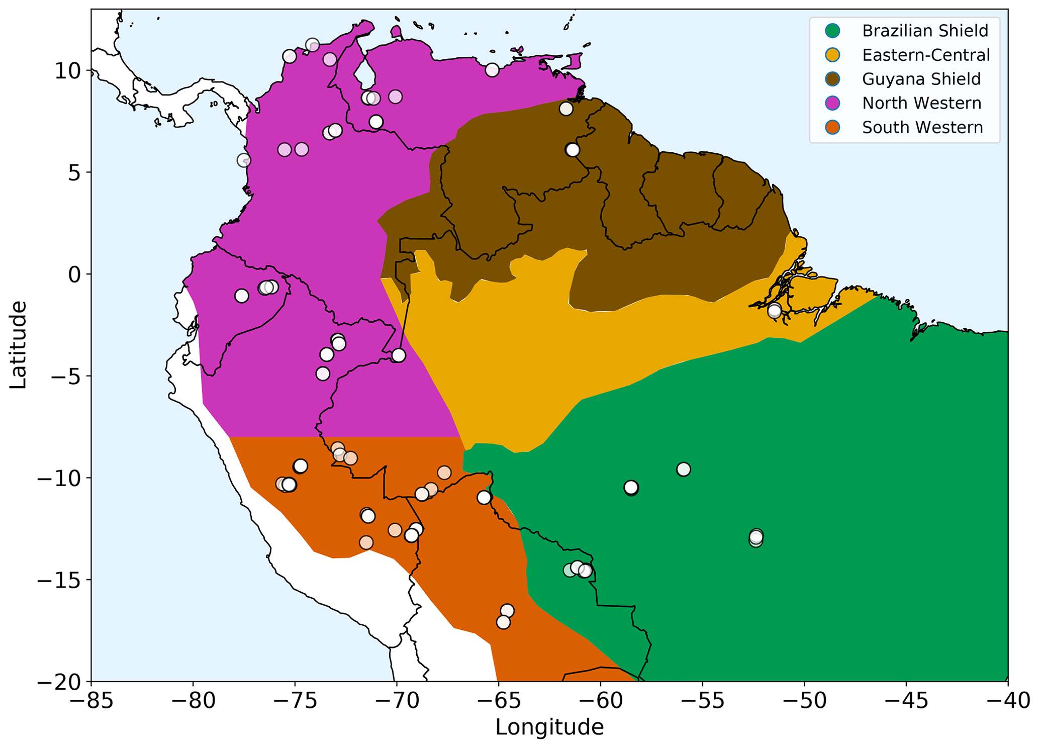
Figure 1 Amazonian allometric regions. Each region, shown by the coloured areas, is defined by geography, rainfall and soil substrate. White circles show location of the forest plots used. The two western regions share common allometry but are split based on rainfall seasonality for analysis purposes.

We selected 124 open-access forest plots (Fig. 1) classified as mixed forest (not monoculture) and old growth to most closely match the model assumptions of forests undisturbed by human interference and approximating to equilibrium demography. The 124 selected plots all had a consistent lower cut-off in measurements at a 10 cm trunk diameter. Two available upper montane plots with very few measurements above 10 cm were not included in the 124 plots used, as they did not have enough measurements to allow for a reliable fit.

3.2 Calculating dry tree mass from trunk diameter

The open-access plots of the Amazon RAINFOR dataset consists only of trunk diameter values. To estimate the tree mass, the methodology developed by Feldpausch et al. (2012) was used. In that study two functional forms (with and without height) were tested against destructively sampled mass data (trees carefully measured then cut down and weighed) to find ones which best estimated mass from trunk diameter. It was found that mass estimation accuracy doubled when including height, even if the height had in turn been estimated from trunk diameter. Out of three choices of height functional form (power law, Weibull-H and exponential), Feldpausch et al. (2012) found the Weibull-H form Eq. (11) to be the best at estimating mass across multiple size classes. The height H in metres is then

$$\begin{array}{}\text{(11)}& H=a_{\mathrm{h}}(\mathrm{1}-\exp (-b_{\mathrm{h}}{D}^{c_{\mathrm{h}}}\left)\right),\end{array}$$

with the coefficients varying geographically between defined allometric regions (see Table S1 in the Supplement and Fig. 1).

The regions were defined by geography and substrate origin (Feldpausch et al., 2012): western Amazonia (Columbia, Ecuador and Peru) being recently weathered Andean deposits, the geologically old Brazilian Shield to the south (Bolivia and Brazil), Guyana Shield on the northern side of the Amazonia basin (Guyana, French Guiana and Venezuela) and Eastern-Central Amazonia (Brazil) consisting of sedimentary substrates originating from the other regions. The western region from Feldpausch et al. (2012) was split along latitude of −8^∘ based on rainfall seasonality (Fauset et al., 2015). These two western regions still retain a common height allometry but are split for analysis.

The mass function (kg of tree dry mass), when height was included as one of the parameters used, was

$$\begin{array}{}\text{(12)}& M=e^a({\mathit{\rho }}_{\mathrm{w}}{D}^{\mathrm{2}}H{)}^b,\end{array}$$

where the parameters are universal across all regions with values $a=-\mathrm{2.9205}$ and b=0.9894. The function was from Feldpausch et al. (2011), and the parameters were estimated in Feldpausch et al. (2012).

The wood specific gravity ρ_w was obtained from the Dryad Global Wood Density Database https://doi.org/10.5061/dryad.234/1 (Chave et al., 2009; Zanne et al., 2009). For each tree measurement the ρ_w value used was for that species from the closest available region. Where the species data were unavailable or the species of the measurement had not been recorded, then the ρ_w value of the genus was used, based on an average of all trees in the Dryad database in that genus. Trees without genus data were estimated from family data, and any remaining measurements where the ρ_w was still unknown were set to the average ρ_w of the trees in that same forest plot with known ρ_w values.

3.3 Fitting methodology

As in our previous study (Moore et al., 2018), maximum likelihood estimation (MLE) was used to find the parameters that give the best fit for both the left-truncated Weibull, derived from DET (DET-LTWD), and metabolic scaling theory distributions. MLE is an effective method for parameter fitting of forest size distributions (Taubert et al., 2013; White et al., 2008).

Maximising the log likelihood L results in a more numerically tractable summation of terms rather than a product of terms obtained from using the likelihood directly. L in terms of the probability distribution function (pdf) f(D) is then

$$\begin{array}{}\text{(13)}& L=\sum _i\ln \left(f\right(D_i\left)\right),\end{array}$$

where D_i is tree trunk diameter measurement of stem i in the dataset.

The data were fitted by plot, by allometric region (an aggregated dataset of all plots in that region), and by country (again aggregation of plots), and all the data, from all 124 plots, were grouped together as one large dataset. This allows both the study of the individual plots and the larger-scale patterns across South America.

3.4 Maximum likelihood estimation (MLE) for demographic equilibrium theory

The probability density function f(D) for the DET-LTWD, in terms of tree trunk diameter D and minimum tree size D_L, is related to the number density distribution n(D) (Eq. 4):

$$\begin{array}{}\text{(14)}& \begin{array}{rl}f\left(D\right)& ={\displaystyle \frac{A}{N}}n\left(D\right)\\ & ={\mathit{\mu }}_{\mathrm{1}}{D}^{-\mathit{\varphi }}\exp \left[{\displaystyle \frac{{\mathit{\mu }}_{\mathrm{1}}}{\mathrm{1}-\mathit{\varphi }}}\left(D_{\mathrm{L}}^{\mathrm{1}-\mathit{\varphi }}-D^{\mathrm{1}-\mathit{\varphi }}\right)\right],\mathit{\varphi }\ne \mathrm{1},\end{array}\end{array}$$

where N is the total number of trees in the dataset being fitted, ϕ is the growth scaling power from Eq. (3) and A is the area of the plots containing the trees sampled in the dataset. This equation is equivalent to the standard form of the LTWD:

$$\begin{array}{}\text{(15)}& f\left(D\right)={\displaystyle \frac{c}{\mathit{\lambda }}}{\left({\displaystyle \frac{D}{\mathit{\lambda }}}\right)}^{c-\mathrm{1}}\exp \left[{\left({\displaystyle \frac{D_{\mathrm{L}}}{\mathit{\lambda }}}\right)}^c-{\left\{{\displaystyle \frac{D}{\mathit{\lambda }}}\right\}}^c\right],\end{array}$$

where $c=\mathrm{1}-\mathit{\varphi }$ is the shape parameter and $\mathit{\lambda }={\left[\frac{c}{{\mathit{\mu }}_{\mathrm{1}}}\right]}^{\mathrm{1}/c}$ the scale parameter.

We fit DET-LTWD twice, once with both parameters ϕ and μ₁ allowed to vary as fitting parameters and secondly with the growth scaling parameter ϕ fixed to the MST allometry values ($\mathit{\varphi }=\mathrm{1}/\mathrm{3}$ and ${\mathit{\varphi }}_{\mathrm{m}}=\mathrm{3}/\mathrm{4}$; see Niklas and Spatz, 2004 and West et al., 2009). Fixing ϕ means we have a DET-LTWD model following just one of the two assumptions of MST (the allometry) and so acts as way of comparing the effect of the second MST assumption of space filling when comparing DET-LTWD and MST fits.

3.4.1 One-parameter fit

For this situation, where we are only aiming to find the parameter μ₁ and ϕ is assumed, MLE can then be solved analytically (Kizilersu et al., 2016):

$$\begin{array}{}\text{(16)}& {\mathit{\mu }}_{\mathrm{1}}={\displaystyle \frac{c}{\left(\stackrel{\mathrm{‾}}{D^c}-D_{\mathrm{L}}^c\right)}},\end{array}$$

where $c=\mathrm{1}-\mathit{\varphi }$. The equations are the same for tree mass, just with the symbols appropriately substituted (e.g. m for D).

3.4.2 Two-parameter fit

For the two-parameter case, where both ϕ and μ₁ are fitted, then we calculate the log likelihood L as follows:

$$\begin{array}{}\text{(17)}& L=N\left(\ln {\mathit{\mu }}_{\mathrm{1}}+{\mathit{\mu }}_{\mathrm{1}}{\displaystyle \frac{D_{\mathrm{L}}^c}{c}}\right)-{\displaystyle \frac{{\mathit{\mu }}_{\mathrm{1}}}{c}}\sum _i{D}_i^c+(c-\mathrm{1})\sum _i\ln D_i.\end{array}$$

Substituting Eq. (16) into Eq. (17) creates a function only of one fitting parameter ϕ. This allows for the minimisation of −L in terms of ϕ by using Brent's bounded algorithm (Brent, 1973). Once the optimum ϕ has been found, then μ₁ can be calculated from Eq. (16). As Eq. (16) is included in the minimisation of −L, then it means we are in fact solving for both parameters at once and are finding the maxima of L. This algorithm was tested with both real data and data generated by computer from known LTWD distributions, by plotting the L values against ϕ and μ₁, to confirm the maxima was found correctly (see Figs. S31 and S32 in the Supplement).

Once the parameters μ₁ and ϕ are estimated, this then allows n_L, the tree density per size class at D_L, to be obtained from these parameters and the known quantities of the total number of trees N and the plot area A. This can be derived by integrating the equation for n (Eq. 4) to give

$$\begin{array}{}\text{(18)}& \begin{array}{rl}{\displaystyle \frac{N}{A}}& =\underset{D_{\mathrm{L}}}{\overset{D_{\max }}{\int }}n\left(D\right)\mathrm{d}D\\ & ={\displaystyle \frac{n_{\mathrm{L}}{D}_{\mathrm{L}}^{\mathit{\varphi }}}{{\mathit{\mu }}_{\mathrm{1}}}}\left[\mathrm{1}-\exp \left[{\displaystyle \frac{{\mathit{\mu }}_{\mathrm{1}}}{c}}(D_{\mathrm{L}}^c-D_{\max }^c)\right]\right],\end{array}\end{array}$$

and, noting that the observed number of trees is identical to the integral, we get

$$\begin{array}{}\text{(19)}& n_{\mathrm{L}}=\left({\displaystyle \frac{N}{A}}\right){\displaystyle \frac{{\mathit{\mu }}_{\mathrm{1}}}{D_{\mathrm{L}}^{\mathit{\varphi }}}}{\displaystyle \frac{\mathrm{1}}{\mathrm{1}-\exp \left[\frac{{\mathit{\mu }}_{\mathrm{1}}}{c}(D_{\mathrm{L}}^c-D_{\max }^c)\right]}},\end{array}$$

where $c=\mathrm{1}-\mathit{\varphi }$ and D_max is the largest tree size in the dataset. For this study, it was found that as D_max≫D_L for most cases (and that c is never much larger than μ₁), n_L can be assumed to be

$$\begin{array}{}\text{(20)}& n_{\mathrm{L}}\approx \left({\displaystyle \frac{N}{A}}\right){\displaystyle \frac{{\mathit{\mu }}_{\mathrm{1}}}{D_{\mathrm{L}}^{\mathit{\varphi }}}}.\end{array}$$

Again, the equations are the same for tree mass, just with the symbols appropriately substituted (e.g. m for D).

3.5 Maximum likelihood estimation for metabolic scaling theory

From the equation for number density n (Eq. 8), the pdf for MST is

$$\begin{array}{}\text{(21)}& f\left(D\right)=n\left(D\right)\left({\displaystyle \frac{A}{N}}\right)={\displaystyle \frac{D_{\mathrm{L}}}{\left[\mathrm{1}-\left(\frac{D_{\mathrm{L}}}{D_{\max }}\right)\right]}}{D}^{-\mathrm{2}},\end{array}$$

where D_max is the largest tree size in the dataset. As all the quantities are known, then there are no free parameters to fit and all that needs to be done is calculate n_L, the tree density per size class at D_L:

$$\begin{array}{}\text{(22)}& n_{\mathrm{L}}={\displaystyle \frac{(N/A)}{D_{\mathrm{L}}\left[\mathrm{1}-\left(\frac{D_{\mathrm{L}}}{D_{\max }}\right)\right]}}.\end{array}$$

Similarly the MST pdf for mass from Eq. (9) is

$$\begin{array}{}\text{(23)}& f\left(m\right)=n\left(m\right)\left({\displaystyle \frac{A}{N}}\right)={\displaystyle \frac{\mathrm{3}{m}_{\mathrm{L}}^{\mathrm{3}/\mathrm{8}}}{\mathrm{8}\left[\mathrm{1}-{\left(\frac{m_{\mathrm{L}}}{m_{\max }}\right)}^{\mathrm{3}/\mathrm{8}}\right]}}{m}^{-\mathrm{11}/\mathrm{8}},\end{array}$$

and for n_L it is

$$\begin{array}{}\text{(24)}& n_{\mathrm{L}}={\displaystyle \frac{\mathrm{3}(N/A)}{\mathrm{8}{m}_{\mathrm{L}}\left[\mathrm{1}-{\left(\frac{m_{\mathrm{L}}}{m_{\max }}\right)}^{\mathrm{3}/\mathrm{8}}\right]}}.\end{array}$$

3.6 Estimating plot and regional biomass density

To test the biomass density equations, we used the results of the MLE fits to calculate the biomass density predicted by Eqs. (7) and (10). The biomass density predicted by these equations is then compared to the allometric biomass density (i.e. the sum of the mass of all trees in a dataset divided by the area of the plots). This comparison then provides a goodness-of-fit measure that is relevant to climate.

We chose to measure the biomass density as a function of size in terms of the total mass per unit area from trees with masses equal to or greater than a given size. The main reason for this is that the forest plot data only sampled trees with a trunk diameter equal to or greater than 10 cm. Therefore it makes little sense to measure the biomass density below a given size, as would be the case with a traditional cumulative distribution function. This approach has a second benefit that the mass of a forest above a given size is a much more useful way of easily seeing the contribution of the dominant larger trees to total biomass (Bastin et al., 2018).

A correction term is added to Eqs. (7) and (10) to make sure the biomass density is correctly evaluated at the upper boundary (the mass of the largest tree m_max). This is because these equations only evaluate the mass up to but not including the trees with a mass equal to the largest value in the dataset. Therefore, to comply with the definition above it is necessary to add the mass of the largest trees back into the total biomass.

As the large trees are so rare this correction will be equivalent to adding just one tree of the largest mass m_max in the dataset divided by A, the total area of plots in the dataset.

$$\begin{array}{}\text{(25)}& \begin{array}{rl}{M}_{\mathrm{L}\to max}& =n_{\mathrm{r}}{m}_{\mathrm{r}}^{{\mathit{\varphi }}_{\mathrm{m}}}{\displaystyle \frac{\exp \left(x{\mathit{\mu }}_{\mathrm{m}\mathrm{1}}{m}_{\mathrm{r}}^{\mathrm{1}/x}\right)}{{\mathit{\mu }}_{\mathrm{m}\mathrm{1}}(x{\mathit{\mu }}_{\mathrm{m}\mathrm{1}}{)}^x}}\\ & \left[\mathrm{\Gamma }(x+\mathrm{1},x{\mathit{\mu }}_{\mathrm{m}\mathrm{1}}{m}_{\mathrm{L}}^{\mathrm{1}/x})-\mathrm{\Gamma }(x+\mathrm{1},x{\mathit{\mu }}_{\mathrm{m}\mathrm{1}}{m}_{\max }^{\mathrm{1}/x})\right]\\ & +{\displaystyle \frac{m_{\max }}{A}}\end{array}\end{array}$$

This Eq. (25) is used for all biomass density estimates where the upper bound of tree size is assumed to be finite (based on m_max), while for the cases where the simplifying assumption of infinite tree size is used then Eq. (7) is used.

4 Results

4.1 Mass distribution

When the mass data were estimated from the trunk diameter measurements using the methodology of Feldpausch et al. (2012), it was noticed that the mass size distribution (for all regions and plots) had a peak, which was not present in the trunk diameter distribution. We found this to be an artefact of the conversion from trunk diameter to mass in a distribution that was by definition truncated already in trunk diameter.

Figure 2a shows the relationship between trunk diameter and tree mass for the whole dataset, illustrating that for any particular trunk diameter there is a range of tree masses. This variation in tree mass is caused by the differences in wood density between species and the variation in height allometry between regions (see Eq. 11 and Table S1 in the Supplement). If instead the dataset shown in Fig. 2a is truncated in mass rather than trunk diameter, then the truncation would instead follow the horizontal dotted line and there would be data in the region between that line and the diagonal dotted line. So in effect there are “missing” data for low-mass trees, which is a result of the trunk diameter observations having a minimum sampling size (truncation point) and there being a range of tree masses for trees with a given trunk diameter. This hypothesis is further confirmed by increasing the trunk diameter truncation point, as shown in Fig. 2b. As the truncation point is increased, the peak moves to higher mass.

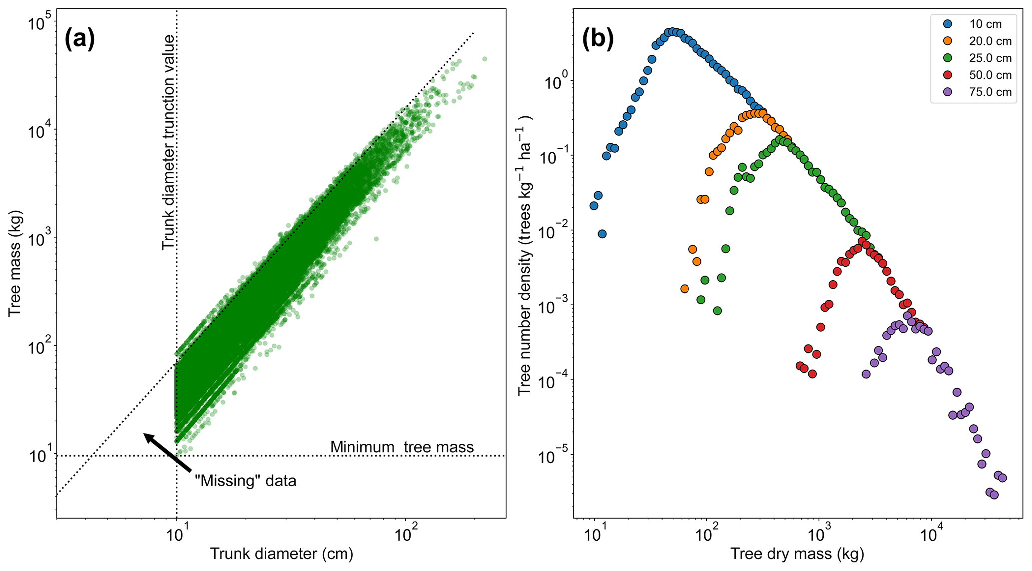
Figure 2 The effect of truncating data measured in trunk diameter and then converting to mass using allometry. In (a), the mass for each tree is shown in terms of its trunk diameter. If the data had been truncated based on mass there would be data in the triangle marked by the intersection of the dotted lines. This truncation effectively leads to missing data in the mass distribution, as seen in (b). The mass distribution should constantly decrease with increasing mass but instead rises to a peak and then decreases due to incomplete data for the low-mass end of the distribution. This peak can be seen to be an artefact of the trunk diameter truncation point. When the trunk diameter truncation point is increased the mass distribution peak moves with the truncation point.

4.1.1 Eliminating the mass peak

When working with mass data the peak was eliminated from fitting by creating 40 bin edges (39 bins) in log space (base e) from the smallest to largest tree in the dataset. These edges define the range of each bin, and the value of each bin was selected as the midpoint in log space. The data were then binned following these bins. Once the data were binned, the bin with the highest frequency was identified. The value of this bin was then used as the truncation point for the dataset when fitting to the dataset distribution. The binning was purely used to identify the peak and for plotting the data and was not used during the MLE fitting process.

4.2 Trunk diameter results

Fitting the DET-LTWD and MST equations to the trunk diameter size distributions showed a consistent pattern for all the geographical aggregations of plot data. In all cases, except Guyana Shield, the DET-LTWD solutions (both one- and two-parameter versions) more closely captured the curvature of the observed size distribution than the MST solution (Fig. 3a and see Figs. S1 and S2 in the Supplement). In particular the MST model deviated from the observed data at large trunk diameters. The Guyana Shield region only had four small plots, totalling 819 trees, which may explain the reason it was hard to visually distinguish the best-fitting model (Fig. S2).

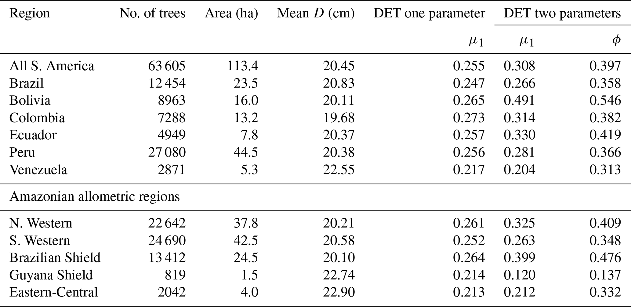
The two-parameter DET-LTWD fits gave a fitted value of the growth scaling power ϕ between 0.137 and 0.546 (Table 1), and 5 of the 12 regions were within 0.05 of the theoretical value of 1∕3 (i.e. ϕ in the range 0.28–0.38).

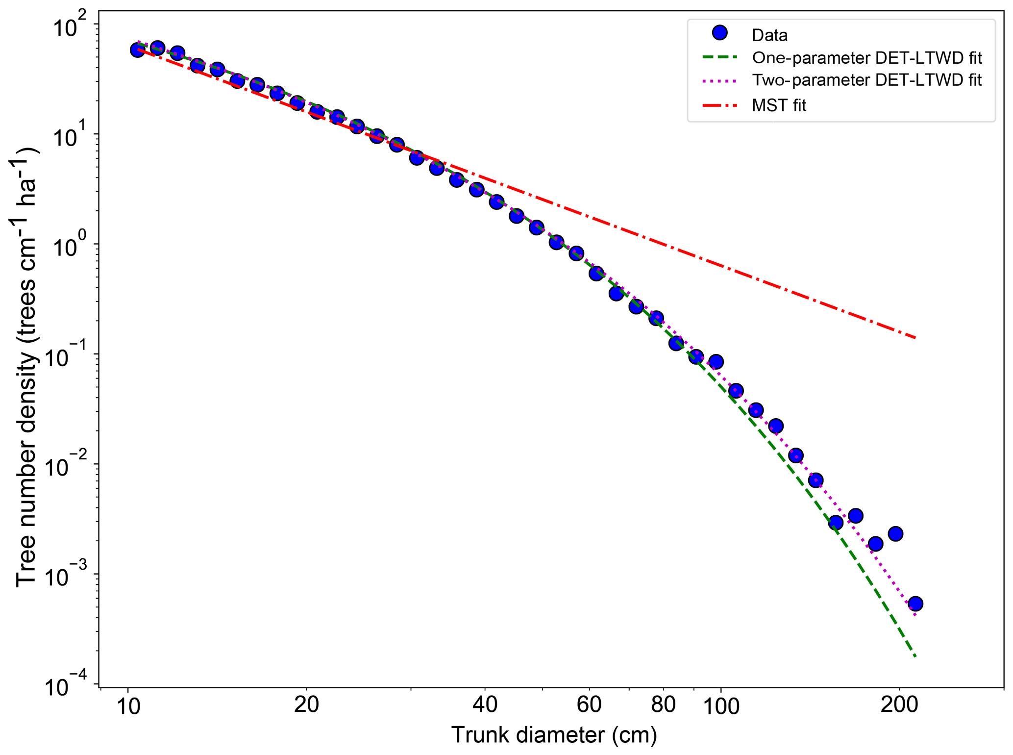
Figure 3 Fit to the trunk diameter size distribution for all South American RAINFOR plots as one large dataset. The blue circles show the binned data and the lines show the fitted distribution for each model.

Table 1 Results of fitting models of the trunk diameter size distributions for the forest plot data aggregated to regions, countries and all plots combined. This table presents the fitted parameters for each model. μ₁ and ϕ are the model parameters from Eq. (3) fitted to the data by MLE. The one-parameter DET model has $\mathit{\varphi }=\mathrm{1}/\mathrm{3}$, so only the fitted μ₁ parameter is given in the table.

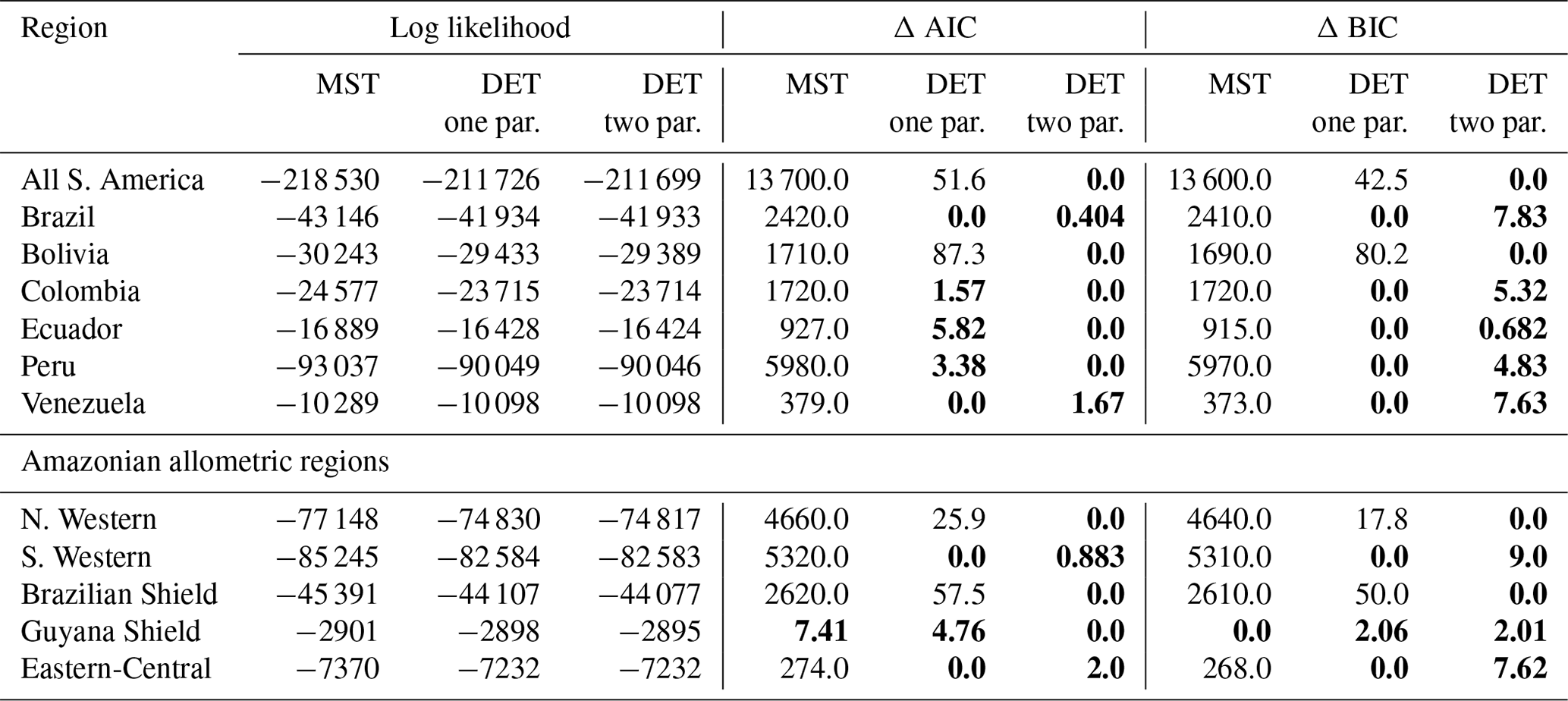
In general the one- and two-parameter DET-LTWD solutions were quite similar in terms of the appearance of the fit on the distribution plots. This finding was confirmed using the Akaike information criterion (AIC) and Bayesian information criterion (BIC) (Table 2). Both the AIC and BIC are a way of determining from several models which has the best goodness of fit, with a lower value indicating a better fit. Both criteria are calculated from the log likelihood and number of fitting parameters, with a difference of 10 being the threshold where the evidence is considered to be very strongly against the higher scoring model (Kass and Raftery, 1995). BIC penalises a higher number of fitting parameters more than AIC.

It was only possible to distinguish the quality of the fits for 4 of the 12 geographical aggregations of forest plots. In all four cases (all S. America, Bolivia, Brazilian Shield and N. Western) the two-parameter DET-LTWD fit was favoured, and for the other eight it was not possible to say that the inclusion of the growth scaling power as a fitting parameter improved the fit.

Table 2 Model comparison for fits to trunk diameter size distributions. This table shows the log likelihood of each model's fit and the corresponding AIC and BIC model comparison criterion. The best model has the lowest AIC or BIC; here the difference is shown compared to the best model, meaning the best model has a score of 0. Models other than the best are strongly rejected if they have a value greater than 10. The best model and those not rejected are shown in bold.

4.3 Trunk diameter results for individual plots

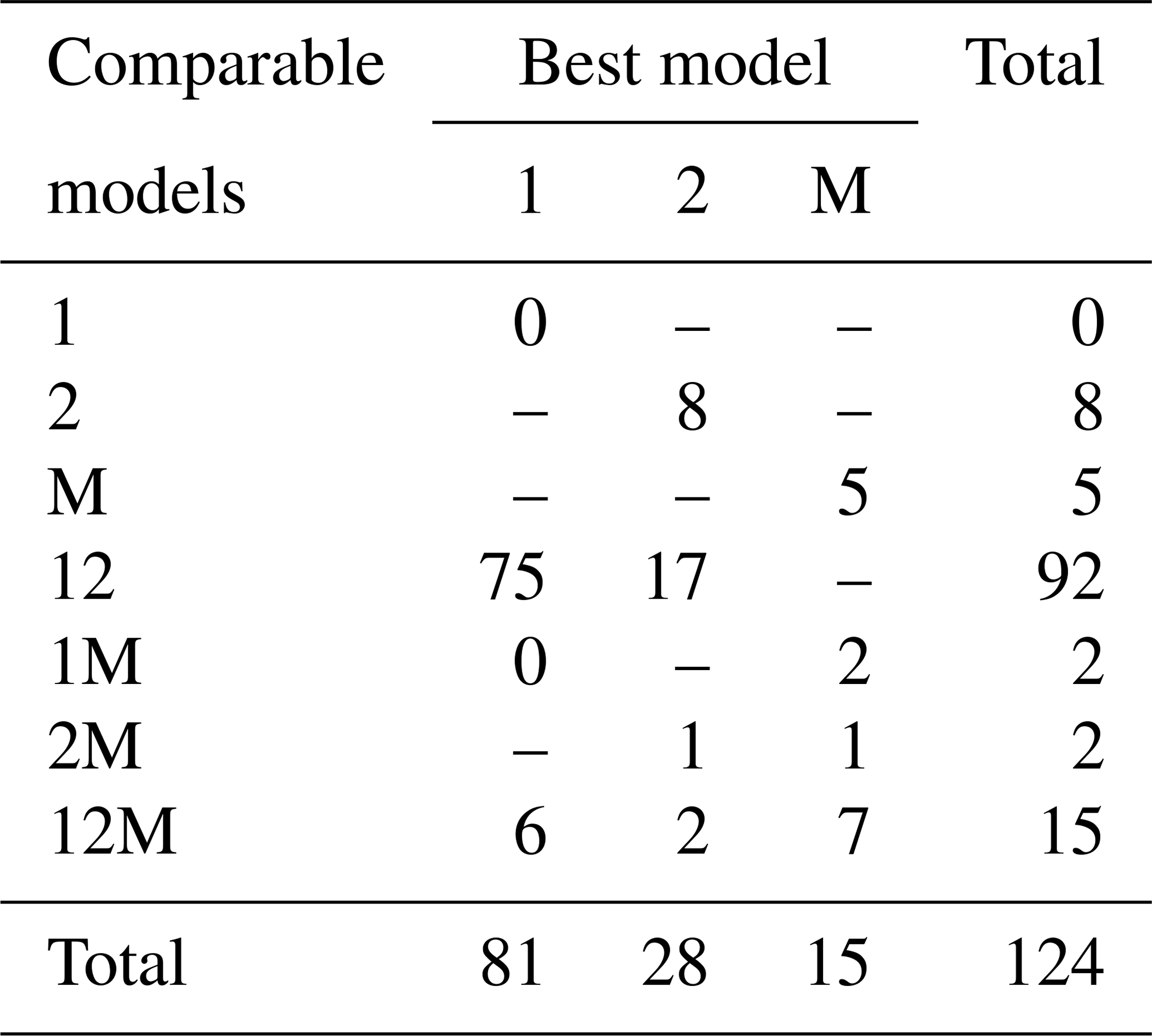
Fitting the models to the individual forest plots (full results in Tables S3 and S4 and Figs. S5 to S13 in the Supplement) again resulted in the DET-LTWD models generally fitting much more closely than MST. Table 3 shows the results of BIC comparison of the models for the 124 forest plots. In every case, the best model is determined by the lowest BIC value. Inferior models are only considered strongly rejected if their BIC is greater than the best model by 10 or more. The number of plots where each model has the best BIC score is represented by the columns in the table and shows the one-parameter DET-LTWD was the model most commonly favoured by the BIC score (81 plots). However, in none of those plots was it possible to strongly reject both of the other models. The most common result (75 plots) was of the one-parameter DET-LTWD being the best model with MST being rejected but the two-parameter DET-LTWD also so closely fitting the data that it cannot be rejected. The next most common result (17 plots) was the reverse with again MST rejected but the two-parameter DET-LTWD now narrowly better but not sufficient to strongly reject the one-parameter DET-LTWD. The MST model was the best model for 15 plots, and for 5 of those (ELD_01, ELD_02, RIO_01, RIO_02, TIP_03) the two DET-LTWD models were both strongly rejected. Four of these plots though had a very low number of trees, so the fitting process would be less likely to be able to pick a model with as much confidence from a distribution of only ∼100 trees. In fact the MST model seemed more likely to have a favourable AIC or BIC score, compared to the other models, for plots with smaller sample sizes and an increasingly unfavourable score for higher sample sizes (see Fig. S30).

Table 3 Shows the best and acceptable models for the 124 individual forest plots for trunk diameter. Models are labelled as “M” for MST, “1” for the one-parameter DET-LTWD and “2” for the two-parameter DET-LTWD. Columns refer to best-fitting model (lowest BIC score). Rows refer to models that are so good a fit compared to the best that they cannot be rejected, as their BIC score is so close to the best model. For example “1M” means the MST and one-parameter models are not rejected but the two-parameter model is rejected based on BIC. Then the columns in this row show how many forest plots have either the 1 or M model as the best fit.

Plotting just the ϕ results in a histogram (Fig. 4a) reveals an approximate bell-shaped distribution with a peak close to the theoretical MST value. The median of the ϕ value for the plots is 0.34 (95 % confidence interval 0.29–0.40), and the mean is 0.31 (95 % confidence interval 0.26–0.36). These values are close to the theoretical value of 1∕3, as suggested by the histogram. The histogram of μ₁ (Fig. 4b) shows a skewed bell-shaped distribution with a peak around 0.3 for the two-parameter DET-LTWD and a more symmetric bell curve centred around 0.25 for the one-parameter DET-LTWD. For the one-parameter DET-LTWD the median of μ₁ for the plots is 0.25 (95 % confidence interval 0.24–0.26), and the mean is 0.25 (95 % confidence interval 0.24–0.26). For the two-parameter DET-LTWD the median of μ₁ for the plots is 0.27 (95 % confidence interval 0.22–0.31), and the mean is 0.31 (95 % confidence interval 0.26–0.35). The one-parameter DET-LTWD mean and median μ₁ are very close to the value of 0.22 found when the one-parameter DET-LTWD was fitted to US forest inventory data (Moore et al., 2018; note that in that study the fitted value of μ=1.198 was obtained for D=12.7 cm, which was then converted, by extrapolation, to the value at D=1 cm to get μ₁ – this value is 0.22).

Figure 4 (a) Results for the growth scaling power ϕ when fitting the two-parameter DET-LTWD via MLE for trunk diameter data from all 124 individual forest plots. The vertical black dotted line shows the value $\mathit{\varphi }=\mathrm{1}/\mathrm{3}$ predicted by MST allometry. (b) Results for the fitted mortality-to-growth ratio μ₁ for both the one- and two-parameter DET-LTWD via MLE for trunk diameter data from all 124 individual forest plots.

Figure 5 shows the effect of fitting with the two-parameter DET-LTWD model. There is a clear relationship between ϕ and μ₁, as all results follow a curve.

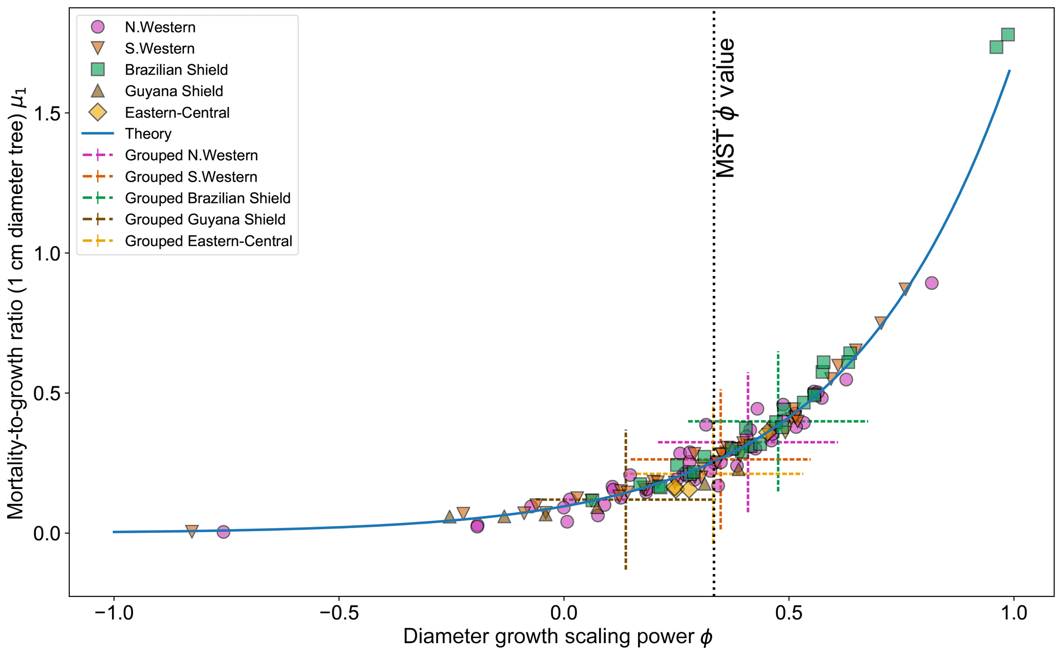
Figure 5 Results of the two-parameter DET-LTWD MLE fits for trunk diameter data from all 124 individual forest plots. The fitted mortality-to-growth ratio μ₁ is shown as a function of the fitted growth scaling power ϕ. The results from the fits to the grouped datasets of the four allometric regions are plotted as the dashed crosses of the corresponding colour. The vertical black line shows the ϕ value predicted by MST allometry. The blue line represents the relationship derived from MLE equations for DET, showing the best fit μ₁ for a given ϕ.

If it is assumed that for any fixed value of ϕ there is a μ₁ value that gives the best fit for that (as can be seen in Fig. 3b), then an equation can be derived (see Sect. S2 in the Supplement) in terms of the DET theory and the known global best-fit values ϕ_t and μ_t1 (i.e. the values fitted to all plots together):

$$\begin{array}{}\text{(26)}& {\mathit{\mu }}_{\mathrm{1}}={\displaystyle \frac{\mathrm{1}-\mathit{\varphi }}{\left(\frac{\exp \left(v_{\mathrm{L}}\right)}{(x_{\mathrm{t}}{\mathit{\mu }}_{\mathrm{t}\mathrm{1}}{)}^y}\mathrm{\Gamma }(y+\mathrm{1},v_{\mathrm{L}})-D_{\mathrm{L}}^{\mathrm{1}-\mathit{\varphi }}\right)}},\end{array}$$

where $x_{\mathrm{t}}=\mathrm{1}/(\mathrm{1}-{\mathit{\varphi }}_{\mathrm{t}})$, $y=\frac{\mathrm{1}-\mathit{\varphi }}{\mathrm{1}-{\mathit{\varphi }}_{\mathrm{t}}}$ and $v_{\mathrm{L}}=x_{\mathrm{t}}{\mathit{\mu }}_{\mathrm{t}\mathrm{1}}{D}_{\mathrm{L}}^{\mathrm{1}-{\mathit{\varphi }}_{\mathrm{t}}}$.

Equation (26) appears to fit the general trend of the fitted values well (Fig. 5), but as can be seen in Figs. S31 and S32 the curves for all plots together and individual plots do not coincide, so it is unclear whether this equation explains the relationship or if it is coincidental. Whether the equation is the true description or not, the relationship between μ₁ and ϕ suggests that there is a possibly that a trade-off as a high-μ₁, high-ϕ tree would have a superior growth : mortality ratio at smaller sizes but an inferior growth : mortality ratio at larger sizes compared to a low-μ₁, high-ϕ tree.

This trade-off would take place in each forest plot with the dominant strategy in each plot depending on local conditions that are affecting growth and mortality. To test if the trade-off could explain the results, fitting parameters μ₁ and ϕ were compared to forest plot properties such as sample size, geographical location, mean plot height, trunk diameter, mass, wood density and basal area. The relationships were generally weak with little correlation, suggesting a poor signal-to-noise ratio or that the metrics used above had little or no correlation to the fitting parameters. So currently it cannot be confirmed that the cause of the relationship is the suggested trade-off, but it remains an interesting possibility.

4.4 Mass results

All fitting was performed on mass data after trees smaller than m_P had been excluded. m_P was chosen based on the methodology in Sect. 4.1.1. When fitting the DET-LTWD and MST equations to the mass size distributions, there was again a consistent pattern for all the geographical aggregations of plot data. In all cases the DET-LTWD solutions (both one- and two-parameter versions) fitted much more closely than the MST solution (Fig. 6 and see Figs. S3 and S4 in the Supplement). Again the MST model overestimated the number of large trees.

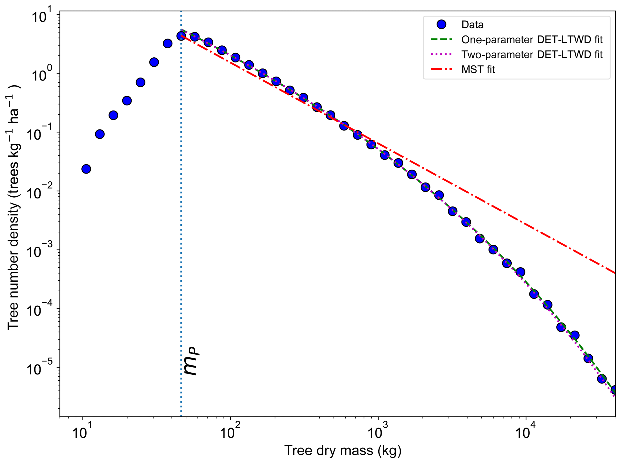
Figure 6 Fit to the mass size distribution for all South American RAINFOR plots as one large dataset. The blue circles show the binned data and the lines show the fitted distribution for each model. The peak in the distribution is clearly shown. The fitting is only performed on trees with mass greater than the mass of the peak.

The two-parameter fits gave a fitted value of the growth scaling power ϕ_m between 0.635 and 0.794 (Table 4) which showed that the growth allometry is close to the theoretical value of 0.75 (10 of 12 regions with ϕ_m in the range 0.7–0.8). The table also shows the truncation point m_P used for each dataset, and all trees with mass less than this value were excluded. The value of m_P corresponds to the peak in distribution created by the conversion from trunk diameter to mass data. The allometric biomass density agrees with the values found previously by Feldpausch et al. (2012), using the same biomass allometry. As this biomass density value is dry mass then it is a reasonable approximation (Chave et al., 2005; Martin and Thomas, 2011) to halve these values to obtain the carbon biomass density, giving a range of 10–15 kg C m⁻².

Table 4 Results of fitting the models of the mass size distributions for the forest plot data aggregated to regions, countries and all plots combined. Shown are the fitted parameters for each model. m_P refers to the point at which all data with smaller mass were excluded to remove the allometry conversion artefact. Biomass is the tree dry mass density of all trees with dry mass above m_P.

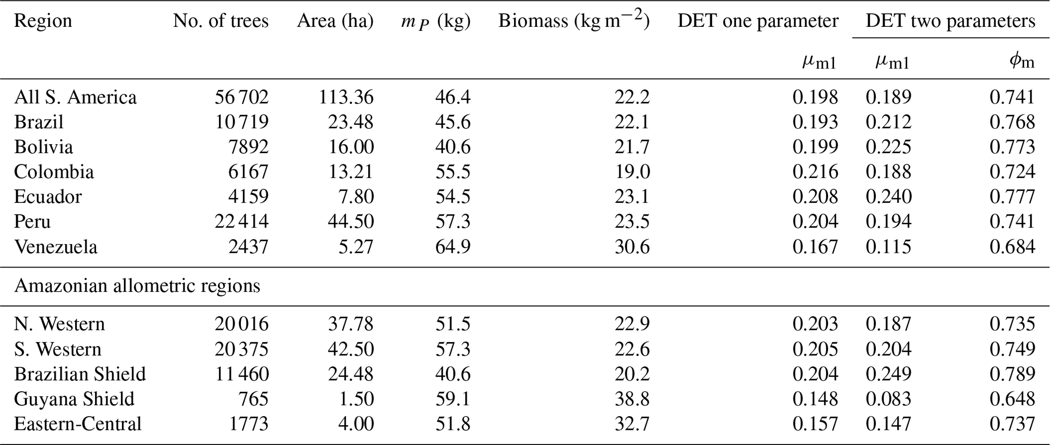
As with the trunk diameter, fits for the two DET-LTWD solutions were, in general, quite similar in terms of the appearance on the mass distribution plots. Again the AIC and BIC fitting metrics were barely able to distinguish which DET-LTWD model best fit the data (Table 5). For nine of the geographical aggregations (all S. America, Brazil, Bolivia, Colombia, Ecuador, Peru, N. Western, Guyana Shield and Eastern-Central) it was not possible to distinguish between the DET-LTWD fits with either AIC or BIC. For Venezuela AIC indicated that the two-parameter fit may be slightly better, but BIC was not able to show any difference. The S. Western allometric region was the only one showing the one-parameter fit as being better but only for BIC. The only region to have both AIC and BIC favouring one of the fits was the Brazilian Shield region, where both AIC and BIC favoured the two-parameter fit.

Table 5 Model comparison for fits to mass size distributions. This table shows the log likelihood of each model's fit and the corresponding AIC and BIC model comparison criterion. The best model has the lowest AIC or BIC; here the difference is shown compared to the best model, meaning the best model has a score of 0. Models other than the best are strongly rejected if they have a value greater than 10. The best model and those not rejected are shown in bold.

4.5 Mass results for individual plots

Fitting the models to the individual forest plots (full results in Tables S5 and S6 and Figs. S14 to S22 in the Supplement) again resulted in the DET-LTWD models often fitting much more closely than MST. All fitting was performed on mass data after trees smaller than m_P had been excluded. m_P was chosen, for each plot, based on the methodology in Sect. 4.1.1. Table 6 shows the results of BIC comparison of the models for the 124 forest plots. In every case, the best model is determined by the lowest BIC value. Inferior models are only considered strongly rejected if their BIC is greater than the best model by 10 or more. The number of plots where each model has the best BIC score is represented by the columns in the table and shows the one-parameter DET-LTWD was the best model by far (80 plots). However, in none of those plots was it possible to strongly reject both of the other models. The most common result (74 plots) was of the one-parameter DET-LTWD being the best-choice model (according to BIC) with MST being rejected but the two-parameter DET-LTWD also so closely fitting the data that it cannot be rejected. The next most common result (14 plots) was the reverse with again MST rejected but the two-parameter DET-LTWD narrowly better but not sufficient to strongly reject the one-parameter DET-LTWD. The MST model was the best model for 15 plots, and for 5 of those (ELD_01, ELD_02, RIO_01, SUC_03, TIP_03) the two DET-LTWD models were both strongly rejected. Three of these plots though had a very low number of trees, so it would be less expected to be able to accurately pick a model from a distribution of only ∼100 trees.

Table 6 Shows the best and acceptable models for the 124 individual forest plots for mass. Models are labelled as “M” for MST, “1” for the one-parameter DET-LTWD and “2” for the two-parameter DET-LTWD. Columns refer to the best-fitting model (lowest BIC score). Rows refer to models that are so good a fit compared to the best that they cannot be rejected, as their BIC score is so close to the best model. For example “1M” means the MST and one-parameter models are not rejected but the two-parameter model is rejected based on BIC. Then the columns in this row show how many forest plots have either the 1 or M model as the best fit.

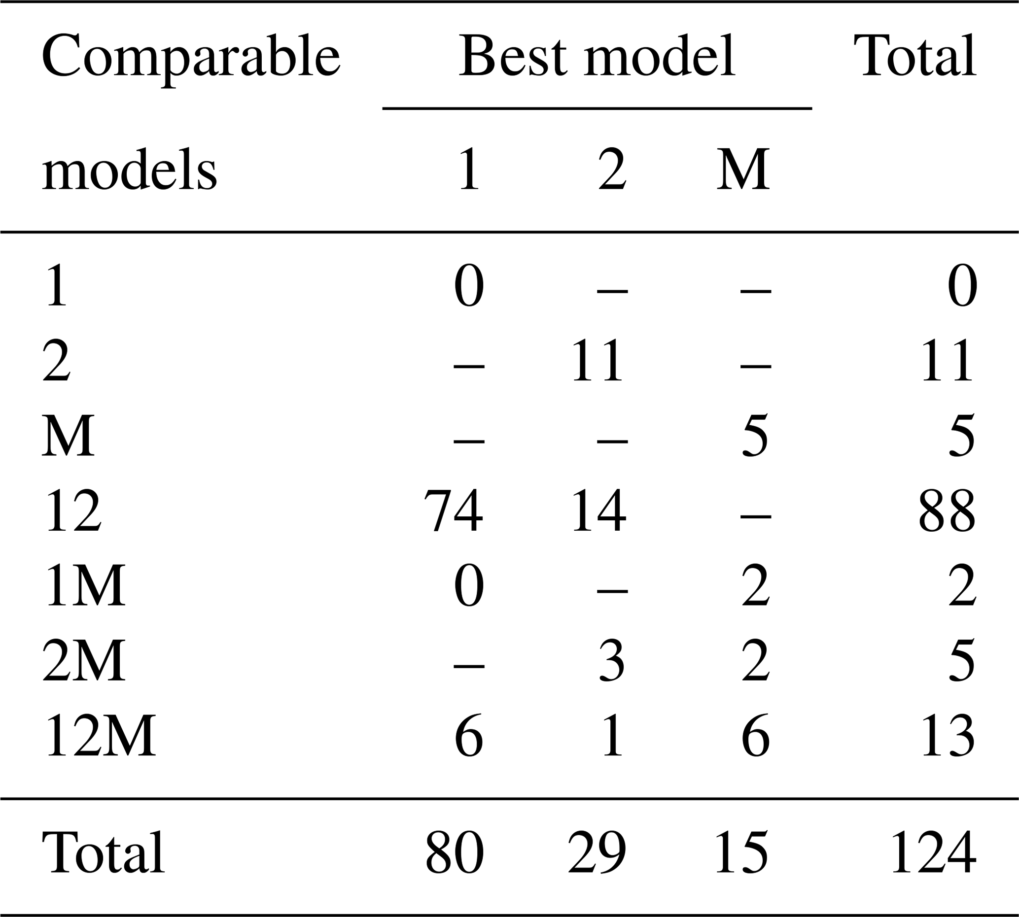
Figure 7 shows the effect of fitting with the two-parameter DET-LTWD model. There is to be a clear relationship between ϕ_m and μ_m1, as all results follow a curve. Equation (26) can be modified to apply to mass and again fits the general trend of the fitted μ_m1 and ϕ_m well.

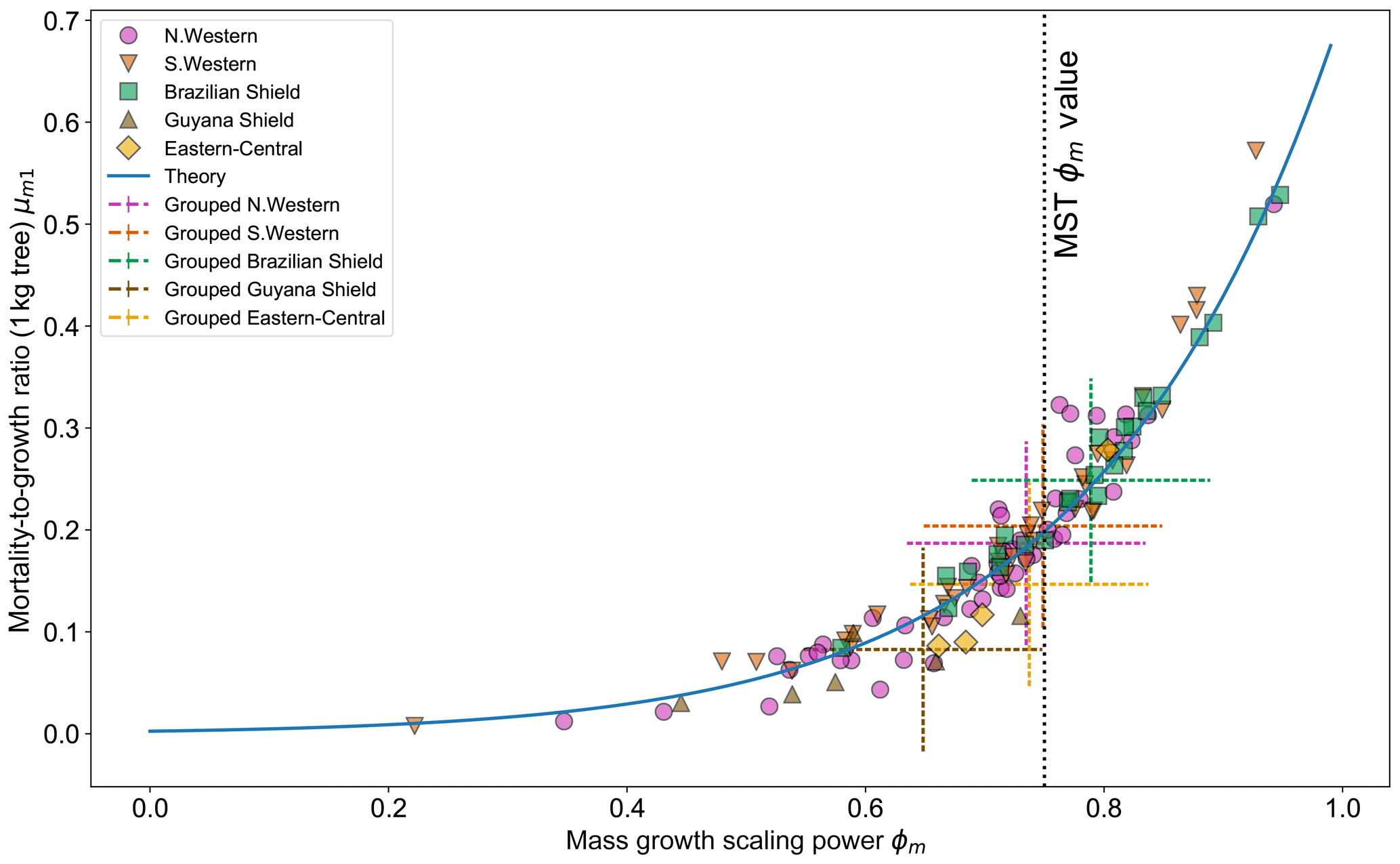
Figure 7 Results of the two-parameter DET-LTWD MLE fits for mass data from all 124 individual forest plots. The fitted mortality-to-growth ratio μ_m1, for each plot, is shown as a function of the fitted growth scaling power ϕ_m. The results from the fits to the grouped datasets of the four allometric regions are plotted as the dashed crosses of corresponding colour. The vertical black line shows the ϕ_m value predicted by MST allometry. The blue line represents the relationship derived from MLE equations for DET, showing the best fit μ_m1 for a given ϕ_m.

Plotting just the ϕ results in a histogram (Fig. 8a) reveals an approximate bell-shaped distribution with a peak close to the theoretical MST value. The median of the ϕ_m value for the plots is 0.72 (95 % confidence interval 0.71–0.75), and the mean is 0.71 (95 % confidence interval 0.69–0.73). These values are close to the theoretical value of 0.75, as suggested by the histogram. The histogram of μ_m1 (Fig. 8b) shows a bell-shaped distribution with a peak around 0.19 for both the one-parameter and two-parameter DET-LTWD. For the one-parameter DET-LTWD the median of μ_m1 for the plots is 0.199 (95 % confidence interval 0.196–0.205), and the mean is 0.198 (95 % confidence interval 0.192–0.203). For the two-parameter DET-LTWD the median of μ_m1 for the plots is 0.177 (95 % confidence interval 0.159–0.205), and the mean is 0.194 (95 % confidence interval 0.174–0.214). It is interesting that for the mass distributions all measures of central tendency cluster fairly closely to 0.19, for both one- and two-parameter fits.

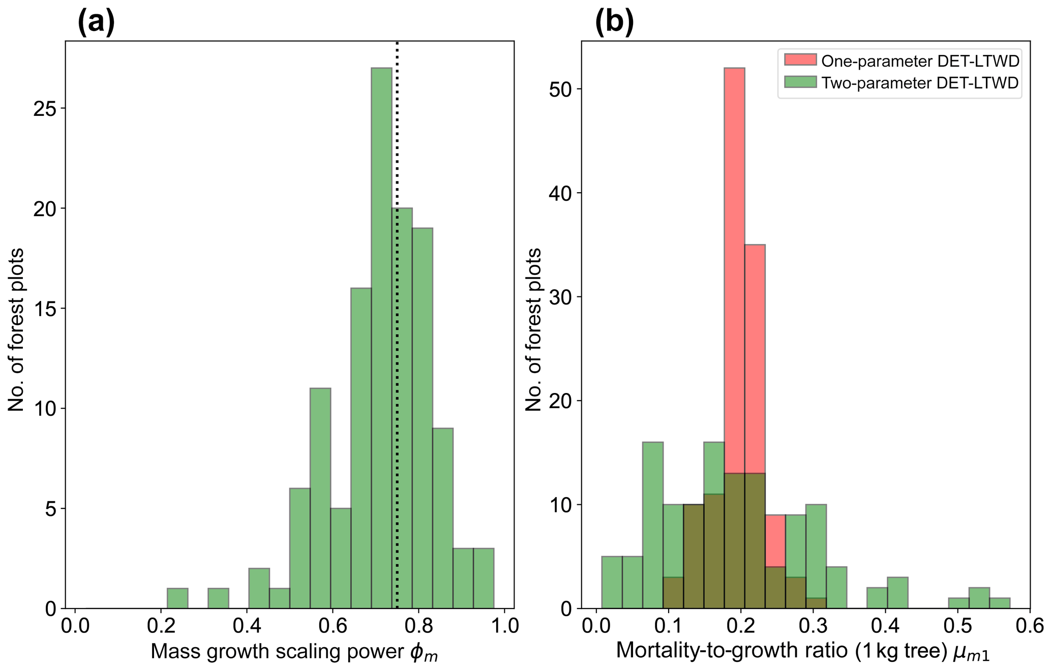
Figure 8 (a) Results for the growth scaling power ϕ_m when fitting the two-parameter DET-LTWD via MLE for mass data from all 124 individual forest plots. The vertical black line shows the value ϕ_m=0.75 predicted by MST allometry. (b) Results for the fitted mortality-to-growth ratio μ_m1 for both the one- and two-parameter DET-LTWD via MLE for mass data from all 124 individual forest plots.

4.6 Biomass results

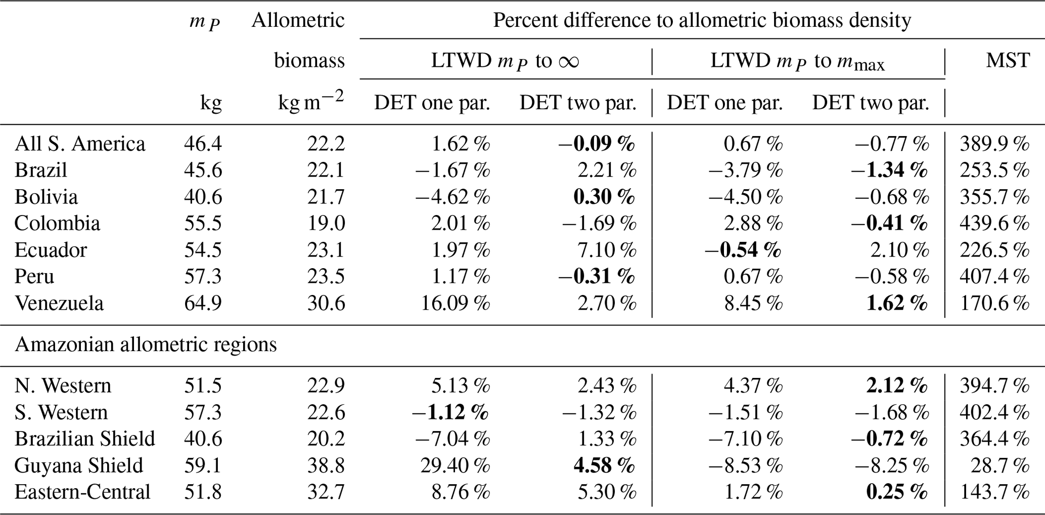
The biomass density Eqs. (6), (7) and (10) were tested against the allometric biomass density (summed tree mass data), as can be seen in Table 7. The biomass density equation parameters were obtained from the fits in Table 4. For the DET-LTWD solutions the biomass density was calculated for both the cases where the upper bound was infinity and the maximum tree mass in the dataset. For each of those cases, the one- and two-parameter DET-LTWD solutions were calculated.

The value of m_P was used for the lower bound for calculating the predicted biomass in Eqs. (6), (7) and (10). The same values of m_P were used to truncate the data when finding the biomass density. So, comparisons between the theory and the mass obtained directly from a combination of observation and allometry were always using the same lower truncation point for each dataset but varied between datasets. The values of m_P used are given in Table 4, and the methodology used to estimate m_P is in Sect. 4.1.1.

It is apparent that the MST biomass density equation is inferior to the DET-LTWD-derived biomass density equation from the DET theory. For all aggregations the biomass density was overestimated by MST, and in many cases by a considerable margin. The comparison of the different DET-LTWD biomass density equations was found to favour the two-parameter fit using the finite upper bound (6 regions out of 12). Four areas had better estimates with the two-parameter fit using the infinite upper bound (all S. America, Bolivia, Peru and Guyana Shield).

Interestingly, two regions (S. Western and Ecuador) had a worse fit for the two-parameter DET-LTWD. The S. Western region, though, fits the biomass within 2 % regardless of the choice of upper bound or DET model, so the very slight difference in the biomass density prediction is almost certainly not significant for this region. When the reverse cumulative biomass density, defined as biomass density of all trees above a given tree mass, is plotted for Ecuador (see Figs. S27 and S28) the error comes from the shape of the tail of the distribution, which is much flatter than theory. This flat tail could be due to it being a region with a smaller number of trees (4159) or could be due to higher mortality for large trees in this region.

Table 7 Model biomass comparison. Table shows the percentage difference between each model of the biomass density predicted by the parameters obtained from fitting the mass distribution using MLE and the allometric mass in the dataset. This comparison is only for data where the tree mass is greater than the peak in the mass distribution m_P. Bold indicates the model that is the closest fit to the allometric value.

4.7 Biomass results for individual plots

To look deeper at the relationship between model choice and predicted biomass density, the analysis was repeated for the individual forest plots. In Fig. 9, the results of the biomass density predicted by the models are shown as a function of the actual allometric biomass density. It can be observed that correcting for the largest tree size in each plot is much better than assuming an infinite maximum tree size and that the one-parameter model does not performs as well for the finite maximum tree size case. This finding is supported by looking at the relative root mean squared error (root mean squared error divided by allometric biomass density) for each model, as shown in Table 8.

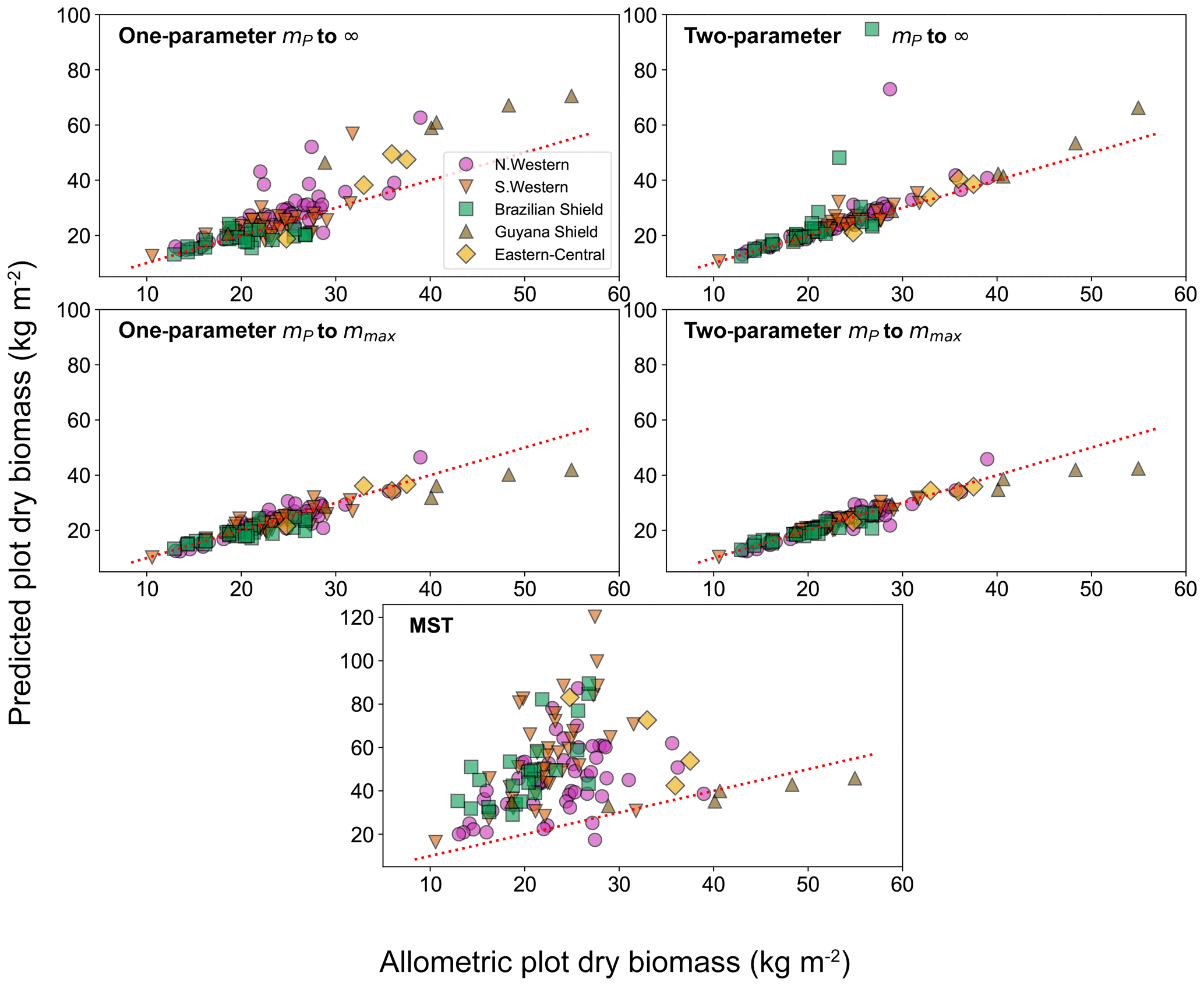
Figure 9 Comparison of the biomass density prediction based on the size-distribution fits to the mass data and to the allometric biomass density in each of the 124 forest plots. Results are plotted for both the one- and two-parameter fits and for both the assumption of infinite and finite maximum tree size. The finite tree size case is limited to the largest tree mass m_max in each forest plot. The red dotted line illustrates the line of a perfect one-to-one relationship (i.e. theory matching the data perfectly).

Table 8 The relative root mean squared error (RMSE) of the biomass density prediction of the 124 forest plots using the parameters fitted via MLE to the mass size distribution. The table compares the results from the different DET-LTWD models and the MST model. The range column indicates the integration limits of the biomass density calculation. The DET-LTWD model assumes no maximum size and by default integrates out to infinity. This can be corrected in terms of the largest tree mass m_max in the dataset.

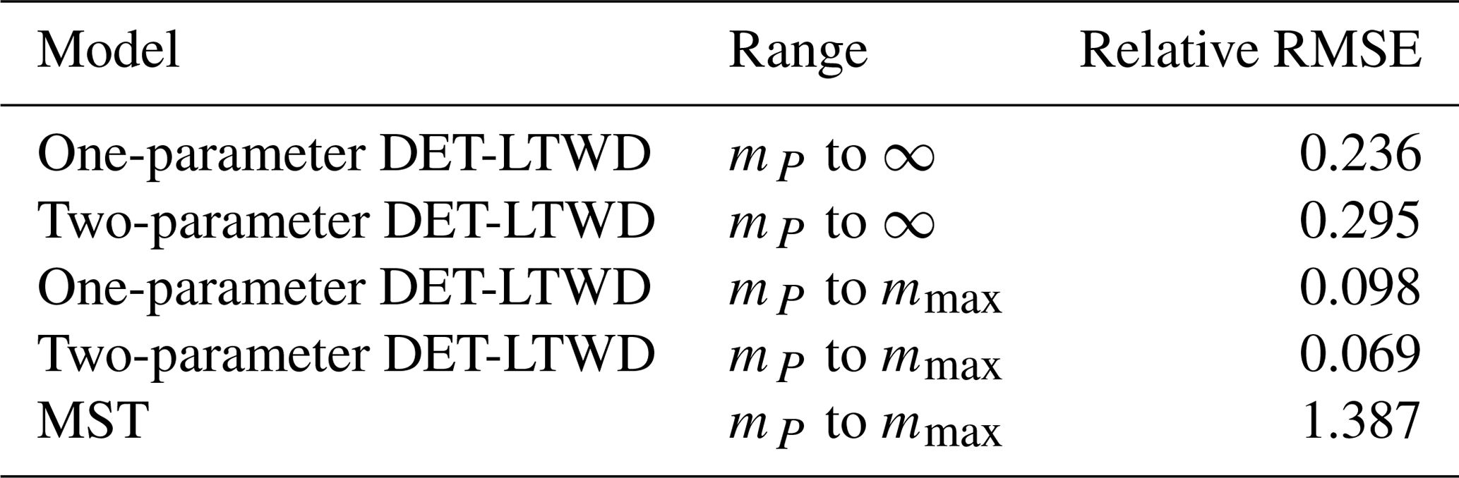
For the small individual forest plots, finite maximum tree size has a larger effect on accuracy than using the two-parameter DET-LTWD over the one-parameter version.

5 Discussion

In this paper we show that the left-truncated Weibull distribution (LWTD), which is consistent with the demographic equilibrium theory (DET) when the mortality is size independent and the growth is a power law of tree size, fits the observed tree-size distributions for 124 forest plots across Amazonia. Our fitting was undertaken with either two free parameters or with one free parameter and the growth scaling power ϕ constrained to that specified in metabolic scaling theory (1∕3 for trunk diameter and 3∕4 for mass; see West et al., 2009; Niklas and Spatz, 2004). We also compared the performance of DET-LTWD to that of the metabolic scaling theory for forest demography (MSTF, West et al., 2009). Our analyses were carried out for both trunk diameter measurements and for trunk diameter converted allometrically to mass (Feldpausch et al., 2012).

We found that this conversion of trunk diameter to mass introduces a peak in the mass distribution that is purely an artefact of the conversion. The peak is due to the variation in mass of trees of a given trunk diameter, due to height and wood density variation leading to some small mass trees being in effect “missing” from the mass distribution. If the diameter-to-mass relationship were purely one to one, then the artefact peak would not occur. This peak has implications for anyone using mass size distributions converted from trunk diameter data. Our solution was to fit only to trees with mass greater than the mass distribution peak.

The model fitting shows that Amazon size distributions are generally better fit by the DET-LTWD-based models than MSTF. The two- and one-parameter DET-LTWD fits were often not significantly different enough from each other for comparison by AIC or BIC (which balance the quality of the fit against the number of unknown parameters) to choose which is the best description of the size distributions. The few plots and regions (including all plots combined) where one model was found to have a significantly better AIC or BIC score all favoured the two-parameter model.

The best-fit growth scaling exponent ϕ varied between plots and regions, but the mean value of ϕ across all 124 plots fell close to the values predicted by MST. For the one-parameter DET-LTWD, best-fit values of μ₁ for trunk diameter cluster tightly around 0.25 (and around μ_m1=0.19 for mass). This is close to the mean value of μ₁=0.22 that we found for North American forests (Moore et al., 2018), hinting at a preferred value of the ratio of mortality to growth across different regions and forest types.

The clustering of ϕ results close to the value predicted by MST allometry (Niklas and Spatz, 2004; West et al., 2009) suggests two possibilities. Either that the clustering represents an underlying “basin of attraction” that is modified by local conditions (Price et al., 2007) or that plots do not meet the model assumptions of growth, mortality and equilibrium, and this in turn somehow leads to this clustering. We cannot say for certain why the plots cluster close to the MST values, but it does lead to intriguing future avenues of study.

It was suggested (Coomes and Allen, 2009; Coomes et al., 2011) that light competition should modify the MST scaling of growth with size. This would mean that for trunk diameter the growth scaling power would vary with size and be greater than the predicted MST value of 1∕3. For our regional fits the fitted power was slightly larger than the MST value of 1∕3 in most cases, but for the individual forest plots, the value was very close to MST with no clear bias. So our results cannot be taken as conclusive evidence of light competition modifying the growth scaling but neither are they completely inconsistent with it.

We find the fitted two-parameter DET-LTWD ϕ values for both mass and trunk diameter also have a well-defined relationship to the fitted mortality : growth ratio μ₁. This relationship does not appear to be a fitting artefact, as if artificial data are generated with known μ₁ and ϕ values off the observed curve the fitting process correctly fits them to the generated values, not the curve seen in this study. This relationship suggests an interesting but as yet unknown property of the Amazon forests but may represent life-history trade-offs (Uriarte et al., 2012). Trees have different strategies such as live fast, die young pioneer species versus grow slow, live long canopy species. This is one possible explanation of the relationship between μ₁ and ϕ, as when both are high the early growth at small sizes will be slower but keep increasing, while when ϕ and μ₁ are both low the early growth will be higher but more quickly level off. Interestingly no plots had a low ϕ with high μ₁, which would correspond to uncompetitive low growth at all sizes. As these results are at the plot level rather than per tree basis, they would suggest that each site has a dominance of one life-history strategy. As there is no correlation of μ₁ or ϕ with plot metrics such as height or wood density, this hypothesis remains unconfirmed.

MSTF was rarely a good fit at the plot, regional or all-plots level for either trunk diameter or mass distributions, and it significantly overestimated total biomass density, so we reject the MSTF model as a good model of forest size distributions. This rejection is consistent with the recent study by Zhou and Lin (2018) that showed the MSTF model failed to account for the effect of the size-dependent growth rate on how fast a tree transitions through a given size class. This observation explains that the assumptions of MSTF of the size-distribution scaling D⁻² are inconsistent with the assumption of individual tree resource use scaling as D². Here, we have confirmed the D⁻² (and $m^{-\mathrm{11}/\mathrm{8}}$) size-distribution model should be rejected for South American tropical forests. Furthermore, for most plots we can reject a general power law distribution, as the distributions observed are rarely linear when plotted in log–log space.

There was a strong correlation between sample size and how likely MSTF was to be considered either the best model or an acceptable model, with small sample sizes favouring MSTF. This correlation suggests that small sample sizes may lead to difficulty in identifying the best model or even wrongly choosing the best model, most likely as rarer large trees are more likely to be absent from a small sample. Meaning, where practical, larger forest plots of at least 1000 stems are desirable when analysing size distributions.

All three models of size distribution were used to predict total biomass density using the integration of the analytical form of their respective mass distributions. One interesting implication of the resulting equations for DET is that mortality and growth only ever appear in the form of the ratio μ₁ and never independently. The ratio of mortality to growth therefore determines the equilibrium state of a forest, while the absolute magnitudes of the individual mortality and growth terms determine the transient effects away from a steady state.

When considering how well the models predicted total biomass density from the fitted size distribution, the biggest source of error at the plot scale is the model assumption of infinite maximum tree size. However, this can be corrected for and allows the one-parameter DET-LTWD to estimate biomass density with a relative root mean square error of 10 % over the 124 forest plots and the two-parameter DET-LTWD within 6 %. Conversely, the MST model consistently overestimated the biomass density, often by a considerable margin. The regional scale, which has larger sample size, showed much better prediction of the biomass density, and the two-parameter DET-LTWD with finite upper bound had the smallest error in biomass density. This suggests the DET-LTWD model is a useful model of biomass for large-scale applications such as being used to initialise a DGVM based on the continuity equation (Argles et al., 2019) or as a climate-relevant measure of goodness of fit.

One of our priorities for further work is to investigate whether the commonality found in the values of μ₁ and the relationship between μ₁ and ϕ is indicative of some form of optimality operating at the forest scale.

6 Conclusions

This study demonstrates that demographic equilibrium theory (DET) is able to fit measured tree-size distributions in Amazonian forests. The fitted growth scaling parameter ϕ was clustered for both trunk diameter (0.31±0.02) and mass diameter (0.71±0.01) distributions close to the values predicted by metabolic scaling theory (MST). The small bias seen could be indicative of deviations from MST allometry due to light competition. The fitted mortality : growth ratio parameter μ₁ was clearly related to the fitted ϕ parameter, suggesting a possible life-history trade-off in the forest plots. If the DET ϕ is constrained to the MST value then the fit is often as good as the two-parameter fit, and with one less fitting parameter it is preferred by the Bayesian information criterion and μ₁ clusters with a value (0.25 for trunk diameter) close to that of 0.22 previously reported for US forests. We therefore find evidence that the one-parameter DET is useful in modelling forests on the global scale, particularly for applications where parameter sparsity is important (Argles et al., 2019). Further support for such applications comes from the model's ability to replicate forest biomass density over large scales, when compared to the data. The relationship between the two-parameter DET μ₁ and ϕ and a common value of the one-parameter DET μ₁ between the US and Amazon may indicate some optimality principle is in play.