Sensitivity of 21st century simulated ecosystem indicators to model parameters, prescribed climate drivers, RCP scenarios and forest management actions for two Finnish boreal forest sites

Forest ecosystems are already responding to changing environmental conditions that are driven by increased atmospheric CO₂ concentrations. These developments affect how societies can utilise and benefit from the woodland areas in the future, be it for example climate change mitigation as carbon sinks, lumber for wood industry, or preserved for nature tourism and recreational activities. We assess the effect and the relative magnitude of different uncertainty sources in ecosystem model simulations from the year 1980 to 2100 for two Finnish boreal forest sites. The models used in this study are the land ecosystem model JSBACH and the forest growth model PREBAS. The considered uncertainty sources for both models are model parameters and four prescribed climates with two RCP (representative concentration pathway) scenarios. Usually, model parameter uncertainty is not included in these types of uncertainty studies. PREBAS simulations also include two forest management scenarios. We assess the effect of these sources of variation at four different points in time on several ecosystem indicators, e.g. gross primary production (GPP), ecosystem respiration, soil moisture, recurrence of drought, length of the vegetation active period (VAP), length of the snow melting period and the stand volume. The uncertainty induced by the climate models remains roughly the same throughout the simulations and is overtaken by the RCP scenario impact halfway through the experiment. The management actions are the most dominant uncertainty factors for Hyytiälä and as important as RCP scenarios at the end of the simulations, but they contribute only half as much for Sodankylä. The parameter uncertainty is the least influential of the examined uncertainty sources, but it is also the most elusive to estimate due to non-linear and adverse effects on the simulated ecosystem indicators. Our analysis underlines the importance of carefully considering the implementation of forest use when simulating future ecosystem conditions, as human impact is evident and even increasing in boreal forested regions.

1 Introduction

The global atmospheric greenhouse gas concentrations are rising, which induces changes in land ecosystem carbon balances, water cycles and their seasonality. However, there is uncertainty in the magnitude of these changes. The rate of the expected concentration rise depends on human actions and the corresponding emission pathways chosen. The pathways presented in the IPCC AR5 report (IPCC, 2014) lead to a radiative forcing of 2.6 to 8.5 W m⁻² in the year 2100. In addition to climate pathways connected to human actions, the variability in the IPCC climate projections is due to model differences and to internal variability in the climate system. Climate sensitivity has proven to be extremely difficult to constrain (Knutti and Sedláček, 2012). The multi-model spread in temperature and precipitation has not been narrowing during the last few years despite substantial model development (Eyring et al., 2019). However, narrowing the uncertainties should not be the only aim and sign of progress in climate modelling. Models improve as more processes are described in detail, which may also introduce new unknown uncertainties. Thus it is important to study what the contributions of different factors to the total uncertainty of examined variables are, as well as how the uncertainty evolves in the future.

The climate models provide drivers for the land ecosystem models. The predictions by land ecosystem models are affected by the driver uncertainties and by uncertainties related to the land surface model itself. Usually, only variability between different models is examined (see e.g. Friend et al., 2014; Nishina et al., 2015), and the uncertainty related to model parameters is not taken into account (Reyer et al., 2016). The unaccounted model processes can lead to significant underestimation of the overall uncertainty (Trugman et al., 2018). Furthermore, the spread in the uncertainty of the model outcome depends on the variable and region investigated. High-latitude ecosystems are predicted to experience significant changes due to climate warming (Schaphoff et al., 2015). The change in seasonality of the ecosystems is predicted to manifest itself via a decrease in snow cover duration, earlier soil thaw and later soil freeze, and a longer growing season (Dye and Tucker, 2003; McDonald et al., 2004; Barichivich and Caesar, 2012). The longer growing season and warmer temperatures are predicted to increase both ecosystem carbon uptake and respiration (Piao et al., 2008), while harmful extremes connected to heat, soil drought and soil excess water are also predicted to become more severe (Ruosteenoja et al., 2017). The evolution of net ecosystem exchange (NEE), defined as the difference between net ecosystem primary production (NPP) and heterotrophic respiration (R_h), is rather uncertain in the future due to opposing drivers and may follow a trend towards net emissions or net uptake.

Forest management in Finland is a strong modifier of ecosystem carbon budgets and usually an unaccounted source of uncertainty in future predictions. The harvesting intensity defines the impact of the management practices on the ecosystem carbon exchange (Korkiakoski et al., 2019). According to Kalliokoski et al. (2018), the future forest productivity in Finland was predicted to increase towards the end of the century. The climate model ensemble predictions were the dominant source of uncertainty for forest productivity, but closer to the end of century the role of emission pathways became more important. Estimation of future development of ecosystem carbon budgets together with impact factors such as management, seasonality and water conditions adds information to the whole ecosystem functioning. Assessment of uncertainties related to carbon budgets and growing season length together with water and snow conditions is important in estimating the forests' ability to provide ecosystem services related to carbon sequestration, wood harvesting, maintaining habitats and promoting nature tourism (Snell et al., 2018; Holmberg et al., 2019).

Here we estimate how biomass, carbon, growing season, water, and snow-related ecosystem indicators and their uncertainties progress in the future. We engage two ecosystem models at southern and northern boreal forest sites – JSBACH is developed to study land surface processes with closely coupled carbon balances and hydrology, while PREBAS is aimed at studying carbon budgets with implementation of forest management. Both models have been previously calibrated for boreal ecosystems (Mäkelä et al., 2019; Minunno et al., 2019) – these calibrations were independent of one another, and therefore the calibrated parameter sets are different. This also gives rise to a different set of examined ecosystem indicators. We estimate the contribution of model parameter uncertainty, climate model variability, representative concentration pathway (RCP) and management actions to the total uncertainty of these indicators. We apply canonical correlation analysis (CCA) to cross-correlate the uncertainty sources with the chosen ecosystem indicators. Finally, we aim to combine the model estimates to determine which are the dominant sources of uncertainty in future ecosystem projections.

Table 1 Composition of JSBACH and PREBAS model simulations: number of parameter combinations (Par), climate models (Clim), RCP scenarios (RCP), management actions (Manag) and sites as well as the total number of 120-year-long simulations.

2 Materials and methods

In this paper we examine the impact of several uncertainty sources on model outputs in a full factorial design, depicted in Table 1. The models were run separately for both sites with all possible combinations of the uncertainty factors. The experiment design resembles that of the CMIP5 simulations (fifth phase of the Coupled Model Intercomparison Project; Meehl et al., 2009; Taylor et al., 2012). Hence, in the same spirit (Swart et al., 2009) we present this work as uncertainty analysis, although parts of the results and discussion will be more akin to sensitivity analysis. We will next give a brief overview of the experiment design, followed by an introduction of the sites and their characteristics, RCP scenarios, and climate models as well as the models used to run the simulations in this study. Finally we will define our ecosystem indicators and the analysis methods.

The JSBACH and PREBAS models were selected for this study because we had recently calibrated them for boreal ecosystems (Mäkelä et al., 2019; Minunno et al., 2019). Thus, we were able to preserve the parameter interdependence by extracting a set of 100 parameter combinations from the calibration chains – instead of merely sampling the parameter values from their marginal distributions. The extraction methods, parameter definitions, and sample mean and deviation are given in Appendix A. It should be noted that model calibration (partially) compensates for inaccurate or missing model processes and other model deficiencies, which is why we do not focus on this subject.

In addition to model parameterisations that reflect the parameter posterior distributions, we use a subset of climate models and representative concentration pathways (RCPs) from the CMIP5 ensemble (smaller set for JSBACH is due to missing bias-corrected variables). We do not assign any particular probabilities (weights) to the different climate models and RCPs, so these scenarios are considered to be equally likely. Additionally, two management actions were used in PREBAS simulations. They were chosen as to represent the current management practises and a modification that aims for near-term carbon sink increase. These two practises are relatively alike, but more intrusive management actions were not included in this experiment to focus the study.

2.1 Sites

The sites used in this study are called Hyytiälä (FI-Hyy; 61^∘51^′ N, 24^∘17^′ E; 180 m a.s.l.) and Sodankylä (FI-Sod; 67^∘22^′ N, 26^∘38^′ E; 179 m a.s.l.); they are respectively located in southern and northern Finland and represent the southern and northern boreal pine forests. These sites can be characterised as boreal evergreen needleleaf forests, where the dominant species is the Scots pine (Pinus sylvestris).

The Hyytiälä site (Kolari et al., 2009) was planted in 1962, after burning and mechanical soil preparation. The soil type is Haplic Podzol on glacial till. The site has an understory of Norway spruce (Picea abies) and few deciduous trees. The maximum measured all-sided leaf area index (LAI) for the Scots pine is 6.5 m² m⁻², the average measured annual precipitation is 709 mm and temperature is 2.9 ^∘C.

The Sodankylä site (Thum et al., 2007) has been naturally regenerated after forest fires and hosts trees ranging from approximately 50 to 100 years of age. The soil type is fluvial sandy podzol. The ground vegetation consists of lichens, mosses and ericaceous shrubs. The maximum measured LAI for the Scots pine is 3.6 m² m⁻², as determined from forest inventories; the annual precipitation is 527 mm; and temperature is −0.4 ^∘C.

2.2 RCP scenarios and climate models

We selected model runs from the CMIP5 project (Meehl et al., 2009; Taylor et al., 2012) following three representative concentration pathways (RCPs) that reach radiative forcing levels of 2.6, 4.5 and 8.5 W m⁻² by the end of the century (Moss et al., 2010; van Vuuren et al., 2011). Throughout the historical period that ends in 2005 the land cover data and the greenhouse gas concentrations corresponding to different RCPs follow common trajectories (Meinshausen et al., 2011).

Climate data for years 1980–2100 were obtained from five global climate models (GCMs; CanESM2, CNRM-CM5, GFDL-CM3, HadGEM2-ES and MIROC5). The climate variables were bias corrected and further downscaled to a $\mathrm{0.2}{}^{\circ }\times \mathrm{0.1}{}^{\circ }$ longitude–latitude grid, similarly to Lehtonen et al. (2016) and Holmberg et al. (2019). The bias correction methods are described in Räisänen and Räty (2013) and Räty et al. (2014). The FMI meteorological observation data, harmonised by kriging with external drift (Aalto et al., 2013), were used as a reference climate for the period 1980–2010 (Lehtonen et al., 2016).

The subset of five climate models was selected because of their good performance in reproducing current climate in northern Europe and because they provided complete data sets for running impact models (Lehtonen et al., 2016). The future wintertime precipitation changes in Finland for the five models in RCP4.5 cover the range of variability depicted by 24 out of 28 CMIP5 models investigated by Ruosteenoja et al. (2016). In summer the precipitation change range is generally narrower than in winter, and the selected models cover the range of roughly half of the 28 CMIP5 models. Winter temperature change shows intermediate values among the 28 models, and the range captures the ranges of change shown by 11 models. In summer the five-model selection represents the range of change depicted by the upper half of the 28 models analysed by Ruosteenoja et al. (2016). CO₂ concentrations from the RCPs 2.6, 4.5 and 8.5 increased monotonously through the calendar years, reaching respective global means of 421, 538 and 936 ppm by the end of the century. PREBAS was run with results from all five climate models and three RCP scenarios, whereas JSBACH simulations included only RCP4.5 and RCP8.5 due to missing bias-corrected climate variables. Moreover and for the same reason, JSBACH was not run with the HadGEM2-ES climate model for RCP8.5.

2.3 The JSBACH model

The JSBACH ecosystem model (Raddatz et al., 2007; Reick et al., 2013) is the land surface component of the Earth system model of the Max Planck Institute for Meteorology (MPI-ESM). We modified the underlying JSBACH model version (specified in the “Code and data availability” section) as in Mäkelä et al. (2019), where the model is calibrated and validated with site level measurements from 10 different evergreen needleleaf forests throughout the boreal zone (including Hyytiälä and Sodankylä). The calibration was done simultaneously on multiple sites to reduce parameter dependency to any single site – the aim of the calibration was to produce a parameter set suitable for the whole boreal zone. We run JSBACH uncoupled from the atmosphere, apply five layers within a multilayer soil hydrological scheme (Hagemann and Stacke, 2015) and utilise the BETHY model for canopy/stomatal conductance control (Knorr, 2000). Additionally, we set the model to effectively use only one plant functional type (PFT), coniferous evergreen trees, which is the dominant vegetation type on the study sites.

The JSBACH model initial state was derived from the end state of several-thousand-year-long regional simulations that equilibrate the soil carbon storages. In addition, the simulations included a simulation-specific spin-up period of 20 years to ensure adequate site level LAI and soil water storages. The spin-up was achieved by running the model through the first 20 years of simulation data, saving the state of the model variables and using them as the initial state for the 120-year-long simulations. This type of spin-up introduces a discontinuity between the initial state and the driving climate, but differences in the examined climate indicators should be negligible.

2.4 The PREBAS model and management actions

PREBAS (Valentine and Mäkelä, 2005; Peltoniemi et al., 2015; Minunno et al., 2019) is a simplified forest carbon and water balance model, which also considers forest growth and management. It calculates photosynthesis (GPP) using a light-use-efficiency (LUE) approach and ambient CO₂ concentration (Peltoniemi et al., 2015; Minunno et al., 2016). Daily gross primary production (GPP) is influenced by soil moisture, radiation, temperature, vapour pressure deficit and precipitation. The model also calculates evapotranspiration (ET) and updates the water balance daily. Mean tree growth is calculated from GPP and respiration at an annual time step, and growth is allocated to different tree organs under assumptions on tree structure (Valentine and Mäkelä, 2005). The model includes tree mortality due to crowding. The growth module annually updates the canopy leaf area index (LAI) for the GPP and ET estimation. In order to estimate soil carbon, the annual litter fall is calculated by the growth allocation module and fed to the Yasso07 soil carbon model (Liski et al., 2005; Tuomi et al., 2009). NEE is calculated annually.

In addition to weather data, PREBAS requires information about the initial state of the simulated forest, defined as soil fertility class, stand basal area, mean height and mean diameter, at an appropriate spatial resolution. This information was extracted from the multisource forest inventory data maps (Tomppo et al., 2014; Mäkisara et al., 2016). The forest resource maps have a 16 m resolution and report the forest data for the year 2015. The model was initialised with forest data extracted for an area of 8 km×8 km centred at the eddy-covariance towers of Hyytiälä and Sodankylä.

Two management actions were used in PREBAS simulations. The business as usual (BAU) scenario follows present forest management recommendations in Finland (Rantala et al., 2011), where trees have to be at least 24–30 cm diameter at breast height (dbh; 130 cm) and of age from 60 to 100 years before harvesting. The delayed ecosystem logging (DEL) scenario aims for the near-term carbon sink increase by increasing the minimum harvesting diameter to 36 cm dbh.

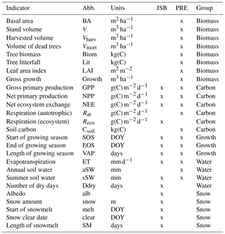
Table 2 Ecosystem indicators derived from the recorded values of the JSBACH and PREBAS simulations, separated into groups for the canonical correlation analysis. The group names relate to biomass distribution, ecosystem carbon exchange, length of the growing season, water cycle and snow melting period.

2.5 Ecosystem indicators and result analysis

We study the uncertainty sources related to key biophysical and biogeochemical indicators and their future development. All simulations, depicted in Table 1, produced daily variables that were used to calculate ecosystem indicators that are presented in Table 2. We have included details on how we calculated the derived variables (number of dry days, as well as start and end days of growing season and snow melting period) in Appendix B.

We analyse the results by producing means, standard deviations and correlations of the model variables. This analysis is based on the annual values or averages over certain months (e.g. summer soil water) – one value per year. We utilise the Mann–Kendall test (Mann, 1945; Kendall, 1975) to verify the existence of trend lines and kernel density estimation (KDE) to visualise the distribution of values (this approach can be viewed as a smoothed histogram).

We also carried out canonical correlation analysis (CCA) to quantify the impact of the different factors on the ecosystem indicators. The factors in this analysis are parametric uncertainty (par), climate models (clim), and RCP scenarios (RCP) for JSBACH and additionally management scenarios (man) for PREBAS. The indicators were averaged and divided into four consecutive 30-year-long periods for both models: 1980–2009 (p1, reference), 2010–2039 (p2, interim), 2040–2069 (p3, mid-century) and 2070–2099 (p4, future). This produced single indicator values for each period and simulation (single instance of each factor) that were calculated for both sites separately.

CCA is a multivariate extension of correlation analysis that allows identifying linear relationships between two sets of variables (Hotelling and Pabst, 1936). We summarise the CCA results with the use of the redundancy index (Rd) that expresses the amount of variance in a set of variables (ecosystem indicators) by CCA uncertainty factors (Stewart and Love, 1968; Weiss, 1972; van den Wollenberg, 1977). In essence, the redundancy index takes into account both correlation and variance between uncertainty factors and ecosystem indicators. The value $Rd\in [\mathrm{0},\mathrm{1}]$, where a higher value indicates that the factor explains more of the uncertainty related to a given indicator (group). There are no general guidelines for the interpretation of the Rd values. Therefore, we examine the resulting indices in relation to one another to reveal relative uncertainties. The details of the CCA and the redundancy index are given in Appendix C.

Figure 1 Redundancy indices for the different uncertainty factors, calculated using all ecosystem indicators using values from 1980–2009 (p1), 2010–2039 (p2), 2040–2069 (p3) and 2070-2099 (p4). Exact values are in the Supplement.

3 Results

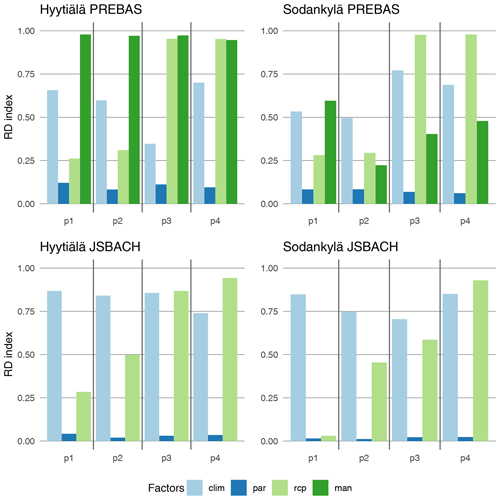
Forest management was the most dominant factor of uncertainty for Hyytiälä (Fig. 1) throughout the simulation. There was a clear difference for Sodankylä, where management gains only half as much influence. Disregarding management, the climate models and RCP scenarios represent major sources of both JSBACH and PREBAS predictive uncertainty. The impact of climate models was dominant during the reference and interim periods and remained roughly constant over time. The importance of RCP scenarios increased towards the end of the simulations, catching up to management impact at Hyytiälä at mid-century and representing the most important factor during the last period. The parametric uncertainty was the least influential factor for both JSBACH and PREBAS at both sites. We will next examine the grouped indicator results.

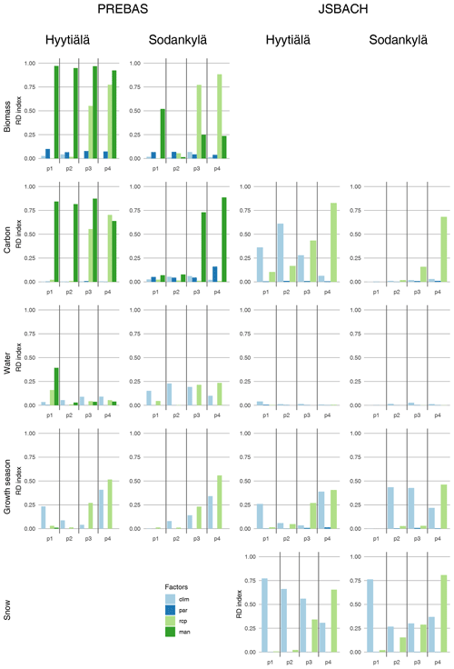
Figure 2 Redundancy indices for the different uncertainty factors, calculated separately for the different indicator groups using values from 1980–2009 (p1), 2010–2039 (p2), 2040–2069 (p3) and 2070-2099 (p4). Exact values are in the Supplement.

3.1 Biomass distribution

The site level differences in biomass stock uncertainties largely arise from the management actions (Figs. 2 and 3), and the management and RCP scenario impacts reflect the redundancy indices calculated with all ecosystem indicators (Fig. 1) for PREBAS. The RCP scenario influence increases for both sites towards the end of the simulations, and the climate model and parameter uncertainty is negligible for both sites and all periods. There is an anomaly for the Sodankylä reference period, where management has a very large impact. This situation arises due to a minimal (0.1 m³ ha⁻¹) but systematic difference in harvested volume – the difference is so small it is not visually evident (Fig. 3). The rest of the Sodankylä reference period variables are nearly identical, so the small change in harvesting results in a high correlation, which is captured by the CCA.

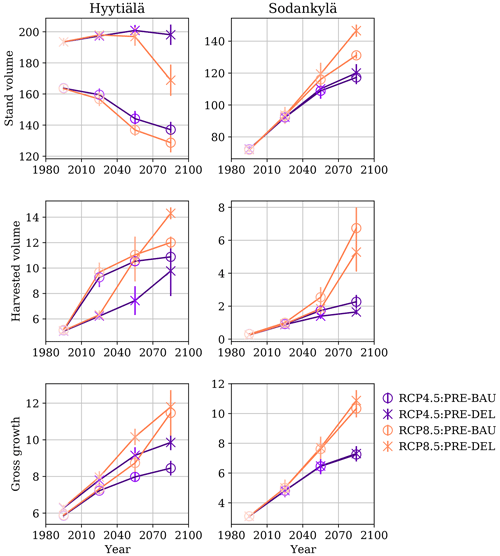
Figure 3 Selected ecosystem indicators from the PREBAS biomass factors, averaged for the 30-year-long periods. The y-axis whiskers at each point represent the point-specific uncertainty: 1 standard deviation amongst the corresponding simulations. We use lighter shading for the earlier periods, a different colour for the RCP scenarios and a different marker to separate the management actions.

The differences in site-specific variables due to the management actions can already be seen from the reference period indicators (Fig. 3). The delayed ecosystem logging (DEL) scenario has an approximately 10 % larger stand volume than business as usual (BAU) for Hyytiälä, but there is practically no difference for Sodankylä. The management actions start to have a noticeable impact for Sodankylä simulated variables at mid-century, but this impact is much smaller than that of the RCP scenarios. The management effect is much more pronounced at Hyytiälä, where both actions follow separate pathways.

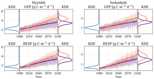
Figure 4 JSBACH predicted annual values of GPP and ecosystem respiration for RCP4.5 (purple) and RCP8.5 (orange) scenarios. The shaded area represents all RCP-specific simulations, the dashed line is the annual mean and the solid line is the trend line. The KDE estimates on the left side of each image represents the distribution of the reference period values of both RCP scenarios (blue), whereas the KDE on the right side consists of RCP-specific values from the last 30 years of simulations.

3.2 Ecosystem carbon exchange

The divergence in the annual GPP and respiration in JSBACH illustrates the separation of the RCP scenarios at about the midpoint (2040) in the simulations (Fig. 4). These two variables that comprise the net ecosystem exchange (NEE) have strong temporal linear correlations for both RCP scenarios (r²≈0.95). The respective linear regression lines for GPP (g C m⁻² d⁻¹) yield an increase of 1.3 and 2.4 (RCP4.5 and 8.5) in 100 years for Hyytiälä and similarly 0.6 and 0.8 for Sodankylä. Likewise, the increases in respiration are 1.6 and 2.6 for Hyytiälä in 100 years and 0.8 and 1.2 for Sodankylä. GPP uncertainty was larger at the beginning of the simulations but levelled with respiration at the end of the period. Relatively, the increased radiative forcing yields a stronger increase in GPP for Hyytiälä and respiration for Sodankylä. Some of the flux variables, such as Sodankylä GPP (Fig. 4), suggest a bimodal value distribution in the last 30 years of the simulations. This is caused by the different climate models yielding separate modes to the otherwise nearly identical value distributions. Most of the GPP and respiration value distribution (Fig. 4) reflect the variation in model parameterisations. This variation is not the parameter uncertainty, which is reflected in how the value distribution changes over time (after removing the effects of the climate models and RCP scenarios).

As the diverging GPP and respiration fluxes signal, the RCP scenarios were important sources of uncertainty for the ecosystem carbon exchange variables at both sites, with importance growing over time (Fig. 2). However, it is noteworthy that management-induced uncertainty for ecosystem carbon exchange was the most influential factor for Hyytiälä when it is accounted for in the model. The Sodankylä flux variation seems to be only dependent on the RCP scenario for both models, while the climate models were the most important factors at Hyytiälä during the first two periods for JSBACH.

3.3 Ecosystem seasonality

The seasonal indicators depict the length of the vegetation active period (VAP) and the snow melting period as well as the amount of soil water (and the recurrence of summer drought). The CCA analysis (Fig. 2) indicates that growing season indicators respond to changes in both climate models and RCP scenarios for both models, but the indicators are not sensitive to management actions. The snow melting period uncertainty for JSBACH is dominated by the climate models for the first half of the simulations for Hyytiälä, after which the RCP scenario is more influential. The situation is a bit different for Sodankylä snowmelt, where the climate model uncertainty reduces radically after the reference period and then remains the same – the RCP scenarios gain effectiveness as simulations progress and reach the climate model influence at mid-century. The uncertainty related to the water balance for JSBACH is not captured by CCA, and the uncertainties for PREBAS are also low.

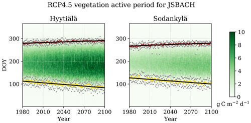
Figure 5 Average vegetation active period for JSBACH RCP4.5; yellow dots are the SOS values, red dots are the EOS values, and the grey dots are the minimum and maximum SOS and EOS from all simulations. Also presented are the trend lines and the daily GPP as the green amplitude.

The vegetation active period is lengthening at both sites (Fig. 5). The displacement of the trend line start of (vegetation active) season (SOS) for JSBACH is approximately −8.1 d in 100 years for Hyytiälä (−11.3 for RCP8.5) and −7.6 d for Sodankylä (−10.9). Likewise, the end of season (EOS) displacement is 3.3 d for Hyytiälä (5.1 for RCP8.5) and 3.5 d for Sodankylä (5.2). The SOS and EOS temporal correlations are typically strong (r²≈0.8). The increase to the length of VAP is very similar for both sites, regardless of the different annual GPP.

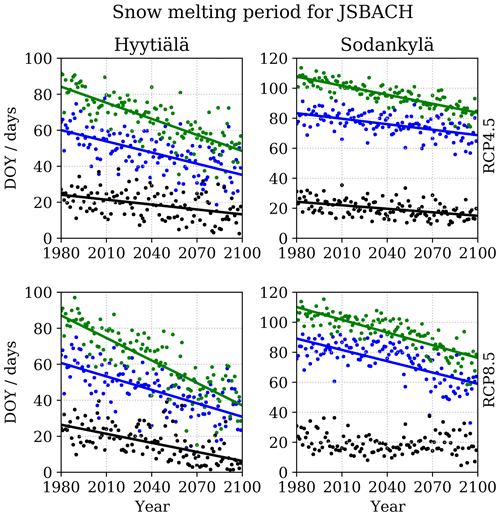
Figure 6 The average snow melting period for the JSBACH model; presented are the average annual values for the start of the snow melting period (blue), the first snow-free day of the year (green), and their difference (black) as well as trend lines (calculated from the shown values) for these variables (when applicable).

The Mann–Kendall tests report a decreasing trend (earlier occurrence) for the start of the snow melting period, first snow-free date and the length of the snow melting period (Fig. 6) in all simulations, except for Sodankylä RCP8.5, where the Mann–Kendall signifies the absence of trend for the melting period length. The simulations indicate that, at the end of the century, the annual amount of snow in Hyytiälä will be radically diminished and that Sodankylä winters will be similar to present-day Hyytiälä winters (especially in the RCP8.5 scenario). Relatively, the first snow-free date is catching up to the start of the snow melting period (Fig. 6). The snow starts to melt approximately 20.7 d earlier in 100 years time for Hyytiälä RCP4.5 and 24.9 d earlier in RCP8.5, whereas the snow-free dates appear 29.8 d (RCP4.5) and 41.7 d (RCP8.5) earlier. The corresponding values for Sodankylä are 12.2 (RCP4.5) and 25.1 (RCP8.5) for the start of the snow melting period and 20.0 (RCP4.5) and 28.2 (RCP8.5) for the snow-free dates. The correlations vary widely: r²≈0.7 for snow-free dates, r²≈0.5 for the start of the melting period and r²≈0.2 for their difference.

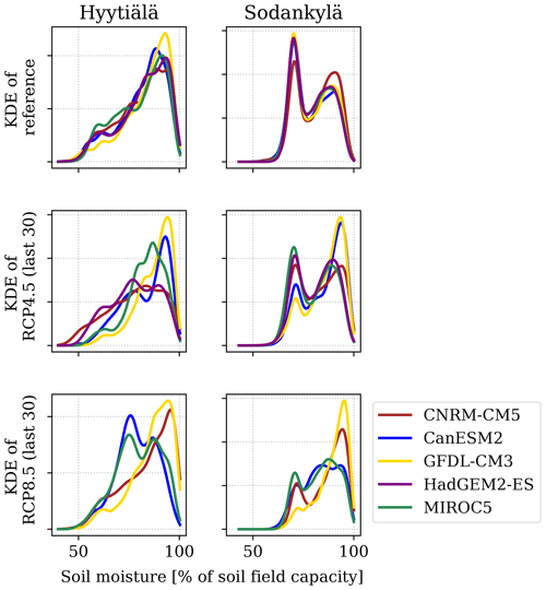
Figure 7 KDE estimates of the JSBACH soil moisture values (relative to soil field capacity) for the reference period and the last 30 years of simulations. Each colour represents the average summertime (June–August) soil moisture, produced with one of the climate models using all parameterisations.

The initial distributions of the summertime soil moisture values (Fig. 7) are unimodal for Hyytiälä and bimodal for Sodankylä for all climate models. This structure is still evident for the RCP4.5 scenario (of the last 30 years) but breaks down for the RCP8.5. Moreover, Hyytiälä RCP8.5 demonstrates some bimodality for two of the climate models, whereas the RCP8.5 for Sodankylä seems to be losing the bimodality and is becoming (in appearance) more similar to the Hyytiälä reference period. The soil moisture value distributions are nearly identical for all climate models at both sites during the reference period, but there are clear differences (distribution modes and shapes) for the last 30 years.

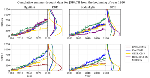
Figure 8 Accumulated summer drought days scatter plotted for each climate model, averaged over model parameterisations with minimum and maximum increment visualised as y-axis whiskers. The grey line is the average of the simulations. The KDE estimates on the right side depict the distribution of the accumulated drought days with the different parameterisations at the end of the simulation. The KDE figures have been cut at 1250 accumulated days.

Table 3 Classification of trends according to the Mann–Kendall test in annual drought days for all simulations.

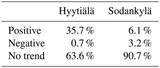
The averaged drought events (Fig. 8) seem to be repeating at a roughly constant rate although the different model parameterisations result in wide soil moisture distributions (Fig. 7) at the end of the simulations. The average cumulative values correspond reasonably well with the drought indicator threshold in Appendix B1 (5 % of 92 summertime days, accumulated for 120 years, would result in 552 d). The temporal correlations for the individual climate model and RCP-specific simulations are poor – Mann–Kendall test for individual simulations indicated some positive, a few negative but mostly no trends (Table 3). The cumulative drought day distributions at the end of the simulations (Fig. 8) are strongly skewed with wide tails and high-value outliers (outside the figures) of approximately 2600 drought days for Hyytiälä and 3700 for Sodankylä. Interestingly, one of the climate models (CNRM-CM5) markedly reduces the amount drought days for the RCP8.5 at both sites when compared to RCP4.5. Neither the accumulated drought day variations nor those of the soil moisture values (Fig. 7) are reflected in the CCA analysis of the Water group (Fig. 2). This is largely a result of low correlation among the simulations.

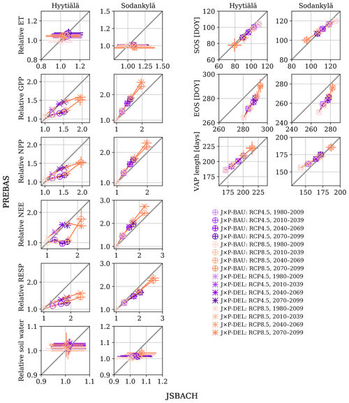
Figure 9 Average simulated values for shared ecosystem indicators between JSBACH and PREBAS, plotted for each 30-year period and both RCP4.5 and RCP8.5 scenarios. The values for JSBACH are divided by the average of the reference period values, and the values for PREBAS are divided by the average of the BAU scenario reference period values. The whiskers at each point represent the point-specific uncertainty: 1 standard deviation amongst the corresponding simulations. We use lighter shading for the earlier periods.

3.4 Ecosystem indicator value comparison

The comparison results (Fig. 9) for soil moisture and ET indicate very small changes in the average values for both models, but the JSBACH simulations manifest substantially larger variation. The JSBACH model yields more elevated levels of relative GPP, NPP, NEE and ecosystem respiration for Hyytiälä, but the situation is (mostly) reversed for Sodankylä. These differences likely reflect the effect of the management actions and distinct site characteristics. The management actions result in clearly different pathways for these variables at Hyytiälä but only yield small differences at the end of the simulation for Sodankylä.

The SOS is roughly identical for both models, whereas both PREBAS versions have a larger effect on the EOS – initially the EOS for PREBAS occurs much earlier (roughly 15 d) than for JSBACH, which is diminished to a few days at the end of the simulations. The PREBAS extends the VAP more evenly from both ends, whereas JSBACH focuses more on the SOS. These differences are reflected in the length of the VAP, which is merely the difference between EOS and SOS. Additionally, we note that the largest value spreads (deviations as represented by the length of the whiskers) appear during the values representing the last 30 years of the RCP8.5 simulations – this merely reflects that the simulation uncertainties are increasing towards the end of the simulation (as expected). Overall, the model responses to the different inputs are very alike, which results in linear dependencies between the variables (Fig. 9).

4 Discussion

In this paper we present an assessment of the importance of the different uncertainty sources, simulated on boreal forests for the 21st century. The JSBACH and PREBAS models yield similar uncertainty estimates (Fig. 1) and have a similar response to many of the examined ecosystem indicators (Fig. 9) when we take into account that PREBAS simulations included forest management. Further differences in modelled variables can be explained by the different model structures (e.g. soil moisture and evapotranspiration). Forest management plays an important role in the estimates of ecosystem variables and their uncertainties. This importance is underscored by the lack of management in many land surface components of climate models.

4.1 Ecosystem indicator sensitivity

According to Grönholm et al. (2018), the long-term eddy-covariance measurements (1997–2017) at a boreal coniferous forest in Hyytiälä indicate a significant increase in gross primary productivity (+10.5 g C m⁻² yr⁻¹), which is only partly compensated by an increased ecosystem respiration (+4.3 g C m⁻² yr⁻¹)). As a result, the annual CO₂ sink has increased by about 6.2 g C m⁻² yr⁻¹. The GPP increase is dominated by an increase in LAI (from 4.1 to 4.6), while the rise in the atmospheric CO₂ concentration (from 360 to 410 ppm) contributes only about 10 % to the rising GPP trend (Grönholm et al., 2018; Wenzel et al., 2016). It has to be noted that Hyytiälä forest was thinned in 2002, temporarily reducing LAI to 3.4. However, in few years the forest recovered to a similar steadily increasing LAI trend to before thinning. The observed rise in the GPP is better replicated by the RCP8.5 scenario (Fig. 4) that yields an increase of +8.8 g C m⁻² yr⁻¹ for Hyytiälä, whereas the increase in ecosystem respiration is more closely reproduced by the RCP4.5 scenario (+5.8).

The RCP scenarios have a strong impact for growing stock and wood harvesting (Fig. 3), but the effect pales in comparison to the examined management actions. This underlines the importance of proper forest management for provisioning services (Snell et al., 2018; Holmberg et al., 2019). This is illustrated by the relative NEE pathways (Fig. 9) that are roughly concave for BAU and convex for DEL management actions. The simulations also indicate linearly lengthening VAP (Fig. 5), with high variation towards the end of the simulations (Fig. 9). This can be interpreted as beneficial for nature tourism and recreational activities, but on the other hand they are the adverse effects of the shortened snow melting period (Fig. 6) and potentially increased droughts (Fig. 8), also investigated by Ruosteenoja et al. (2017). These effects are also detrimental for winter harvesting and wood quality, as suggested by Holmberg et al. (2019).

Manninen et al. (2019) reported lengthened snow melting periods for some regions in Finland for 1982–2016. We analysed the reference period (1980–2009) snowmelt in more detail and found that roughly 30 % of parameter-specific simulations for Hyytiälä and 20 % for Sodankylä resulted in increased length for the snow melting period. We note that our simulations are restricted to the site level, whereas regional experiments include lakes and rivers that can significantly affect the outcome – this type of an uncertainty source is not considered in our simulations.

4.2 Simulation uncertainty sources

The overall uncertainty associated with the management actions differs for Hyytiälä and Sodankylä (Fig. 1). This is due to the more abundant harvesting effect at Hyytiälä (Fig. 3), whereas most of the biomass in Sodankylä is left to grow. Sodankylä stand volume increases as simulations progress, whereas Hyytiälä stand volume remains the same or even decreases for the BAU scenario. This underlines the importance of proper forest management, as the impact of these relatively similar actions is strong – especially when put into context for clear cuts.

As expected, the uncertainty related to the RCP scenarios increases systematically (Ruosteenoja et al., 2016) for all ecosystem indicators and grouped variables (except for the Water group) as the simulations advance further in time. This is similar to results by Kalliokoski et al. (2018). The RCP scenarios are the most dominant factor in explaining the JSBACH and PREBAS uncertainties for both sites at the end of the simulations. The RCP uncertainty also dominates the Carbon, Growth, and Snow variables at both sites and the Biomass variables for Sodankylä. The RCP scenarios tend to gain effect at mid-century (e.g. Fig. 3), although there are some earlier affects, e.g. snow variables for Sodankylä (Fig. 6).

The effect of the climate models on the redundancy indices is the most varied among the examined uncertainty sources. The climate models tend to have more impact in the two earlier periods, although the overall climate model uncertainty remains roughly the same throughout the simulations. This can be seen to reflect the internal variability of the climate system (Knutti and Sedláček, 2012) and the consequent variation in the climatic drivers. The combined variation of climate models and model parameters may not be fully captured due to non-linearity within the simulated variables. This is noted to emphasise the importance of the parameter uncertainty, as stated by Reyer et al. (2016). The parameter uncertainty is expected to be small when compared to the selected RCP scenarios that have a significant impact on the ecosystem (see Holmberg et al., 2019, Fig. 2). Most of the indicator value distributions, induced by the parameterisations, are highly alike for all climate models (Fig. 4), especially during the reference period (Fig. 7). The combined climate model and parameter uncertainty is on par with the RCP scenario uncertainty towards the end of the simulations (Fig. 1).

4.3 Validity of estimates

The JSBACH model calibration (Mäkelä et al., 2019) was originally used in the comparison of various submodel components (stomatal conductance functions), and the PREBAS calibration (Minunno et al., 2019) utilised permanent growth and yield experiments. Both of these examinations rely on hindcasting with relatively recent meteorological measurements or datasets, and the resulting parameter distributions emulate the current climate conditions well. The JSBACH model was calibrated with data throughout the boreal zone, and the parameterisations can be viewed as representing all evergreen coniferous forests, whereas the PREBAS model was extensively calibrated for the whole of Finland. The sites in this study are representative of southern and northern boreal pine forests, and the ecosystem indicators were chosen to reflect the calibrated parameters and processes. We note that model calibration and the parameter distributions also compensate and reflect for missing and imperfectly modelled processes.

The CCA analysis and model comparison focuses on the relative differences in the ecosystem indicators, and thus less importance is given to the absolute indicator values. The CCA analysis only accounts for linear dependencies (Hotelling and Pabst, 1936) between the input and output uncertainties, and even though the redundancy index (Stewart and Love, 1968) considers the (correlated) variance between the variables, the non-linear effects may be underestimated. We reduce the annual variation and linearise the variables by averaging and separating them into four consecutive 30-year-long periods. Additionally, we also examined the PREBAS redundancy indices without the RCP2.6 – these results differ only marginally from those with the RCP2.6 included, which increases the validity of the JSBACH results.

This linearisation may not be enough to capture all variation, as is the case with the JSBACH Water group uncertainties (Fig. 2) and the wide spread of soil moisture values (Fig. 7) and cumulative drought days (Fig. 8). The different parameterisations and climate models have a prominent variation, but due to adverse effects the correlations remain small. For example, the RCP8.5 radically increases precipitation (see Ruosteenoja et al., 2016, Fig. 2) and therefore increases the soil moisture (Fig. 7) and reduces the amount of drought days (Fig. 8). The strength of this effect varies among the climate models, but the model parameterisations still enable even radical increases to the number of drought days. This major source of uncertainty, investigated by for example Trugman et al. (2018), is not captured by CCA. However, when the indicators are reasonably correlated (as is the case for most of the presented indicators), the CCA method is applicable.

The CCA analysis was performed for indicator groups to ensure robustness of the approach – this was not successful in every case, as a minimal but systematic difference in Sodankylä reference period harvested volume led to a large management scenario impact (Fig. 2). The situation arises as all of the other indicator values were nearly identical, and thus a small systematic change that was relatively large had high correlation and impact in CCA. This event was not replicated with the other groups.

5 Conclusions

Although this study is limited to only two sites, our simulations indicate that the management actions have the greatest influence on simulated ecosystem indicators in Finland. When taking into account that the considered management actions are very alike, more emphasis should be given to forest management when simulating future ecosystem conditions. Towards the end of century, the RCP scenarios achieve a similar impact to the management actions. The combined climate model and parameter uncertainty is also an important factor for the whole duration of the simulations due to internal variability of the climate system, but these effects can be easily underestimated due to non-linear or adverse effects. The examined uncertainties are comparable for both models.

Long-term measurements and simulations indicate considerable increases to GPP and ecosystem respiration, with a slightly larger emphasis respectively for the southern and northern boreal forests. While the effect of management on these variables is linear, the impact on NEE is more complex and would be of interest in further studies. The snowmelt is occurring several weeks earlier in all simulations and the length of the snow melting period appears to be decreasing, although the results for Sodankylä are not conclusive. Similarly, the length of the vegetation active period is expected to increase linearly for both sites by a few weeks. Sodankylä soil moisture is expected to increase, while the effects for Hyytiälä are varied. The scenarios do not constrain the recurrence of drought as the parameterisations enable varied outcomes.

We have successfully estimated the roles of different uncertainty sources on overall ecosystem indicator sensitivity at representative boreal forest sites. The study provides material to steer further analysis to relevant uncertainty sources as well as justification to further examine the effect of forest management. The analysis of results is based on CCA that is able to capture the uncertainties when the outputs are correlated. The linearity assumptions in CCA limit its applicability, so other methods, e.g. random forest as in Augustynczik et al. (2017), should also be considered in cases with highly non-linear variables. The uncertainty analysis would also benefit from a larger model ensemble with different model process implementations. In such a case, instead of different model parameterisations, the factorial design could be extended to include different model components or parameterisations representing different functionalities or local management practices. This would still keep the number of simulations reasonable while allowing for a robust uncertainty estimation.

Appendix A: Model parameters

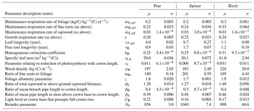
Pre-existing JSBACH and PREBAS model calibrations (Mäkelä et al., 2019; Minunno et al., 2019) were deemed suitable to represent parameter uncertainties in the simulations described in this paper. A set of parameter values was extracted from the model calibrations to preserve parameter interdependence. The PREBAS parameter values were drawn at fixed intervals from the MCMC chains in Minunno et al. (2019). This is a standard approach that results in an approximation of the parameter posterior distributions. The JSBACH calibration was done with adaptive population importance sampling (APIS), which produces a posterior estimate at each iteration. The estimate at 20 iterations (40 parameter combinations) was complemented with 15 additional combinations at each of 40, 60, 80 and 100 iterations. All parameter descriptions, as well as sample means and deviations, are given in Tables A1 and A2.

Table A1 JSBACH model parameter descriptions as in Mäkelä et al. (Table 2; 2019) with distribution mean and standard deviation.

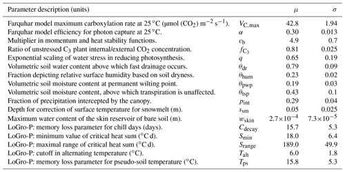
Table A2 PREBAS model parameter descriptions as in Minunno et al. (Table 1; 2019) with distribution mean and standard deviation.

Appendix B: Calculation of ecosystem indicators

Most of the ecosystem indicators in this paper are directly produced by the models, but a few are derived from other variables.

B1 Drought days

The drought days are calculated as the amount of days when average soil moisture (of the combined second and third soil moisture levels in a five-layer JSBACH scheme) is below a certain threshold. Only summertime (June, July, August) values are used, and the threshold for Hyytiälä was set as the 5th percentile of all soil moisture values during the reference period. This value is approximately 33 % of the soil field capacity in Hyytiälä, which compares well with the parameters θ_tsp and θ_pwp for the Hyytiälä drought period optimisation in Mäkelä et al. (2019). Thus, the number of dry days is a reasonable measure for Hyytiälä. We used the same percentile to set a similar value for Sodankylä, although the site characteristics differ (e.g. different soil compositions and field capacity).

B2 Vegetation active period

The dates for the start of season (SOS) and end of season (EOS) for the vegetation active period are calculated from simulated daily GPP. First we extracted the value corresponding to the 90th percentile of the daily GPP, from all of the simulations during the reference period, and then multiplied this value by 0.15. The SOS date is considered to be the first day of the year (DOY), when the daily GPP is consistently above this threshold. The consistency here means that, when we consider the daily GPP values, starting from the 30th DOY to twice as far as the date of the SOS event, the GPP must be above the threshold for at least half of the days. The date for EOS is calculated similarly, when GPP is below the threshold and starting from the 230th DOY.

B3 Snow melting period

The snow depth in model simulation varies on a year-to-year basis. We also encounter some years without any snow cover for Hyytiälä. Hence we first aggregate the snow depth over the model parameterisations and climate model simulations to produce average site and RCP-scenario-specific time series. This approach yields robust estimates of the snow cover, where the actual time series is smooth enough to allow calculation of the beginning of the snow melting period and the first snow-free date. We take a similar approach to that in Manninen et al. (2019) and fit a sigmoidal function to identify the starting date of snowmelt. The snow is considered to have melted when the snow cover has consistently vanished. This means that there is no snow cover for at least half of the days during ±10 d of the snow clear date.

Appendix C: Canonical correlation analysis

We carried out canonical correlation analysis (CCA) to quantify the impact of the different factors on the ecosystem indicators. These factors are parametric uncertainty (pars), management scenarios (man), climate models (clim) and RCP scenarios (RCP). CCA is a multivariate extension of correlation analysis that allows identifying linear relationships between two sets of variables (Hotelling and Pabst, 1936). Its use is similar to multiple regression, but it is more appropriate when there are multiple intercorrelated variables such as model outputs. A more detailed description of CCA is provided in Stewart and Love (1968).

We consider two sets of variables, $X\in {\mathbb{R}}^{n_{\mathrm{f}}\times s}$ (the different factors) and $Y\in {\mathbb{R}}^{n_{\mathrm{e}}\times s}$ (ecosystem indicators), where n_e and n_f are the number of factors and ecosystem indicators and s is the number of simulations, presented in Table 1. Each factor $f_i,i\in \mathit{\{}\mathrm{1},\mathrm{\dots },n_{\mathrm{f}}\mathit{\}}$, or indicator $e_j,j\in \mathit{\{}\mathrm{1},\mathrm{\dots },n_{\mathrm{e}}\mathit{\}}$, can be interpreted as a row vector of X or Y, respectively. In CCA we construct linear composites of the input factors ($U_{\mathrm{1}}=a^{T}X,a\in {\mathbb{R}}^{n_{\mathrm{f}}}$) and output variables ($V_{\mathrm{1}}=b^{T}Y,b\in {\mathbb{R}}^{n_{\mathrm{e}}}$). We choose a and b to maximise the (canonical) correlation (Rc₁) between the composites U₁ and V₁:

$$\begin{array}{}\text{(C1)}& R{c}_{\mathrm{1}}=\mathrm{corr}(U_{\mathrm{1}},V_{\mathrm{1}}).\end{array}$$

This forms the first pair of canonical variates U₁ and V₁. The second pair is formed similarly but it is required to be uncorrelated with the first pair (and so forth for the following pairs). The first pair accounts for the highest amount of variance between the two sets of variables and has the highest canonical correlation ($R{c}_k,k\in \mathit{\{}\mathrm{1},\mathrm{\dots }{n}_k\mathit{\}}$) – the variance and correlations diminish for each consecutive pair. In our analysis, we use three pairs for JSBACH (n_k=3) and four pairs for PREBAS (n_k=4).

The simple linear correlations between an independent variable (f_i or e_j) and a respective canonical variate (V_k or U_k) are called canonical loadings (CL_ik,CL_jk). Similarly, the correlations between an independent variable and its opposite canonical variate (f_i and U_k or e_j and V_k) are called canonical cross loadings (CcL_ik,CcL_jk). To summarise the CCA results via the use of a redundancy index (Rd), we need the canonical loadings of the ecosystem indicators (CL_jk) and canonical cross loadings of the uncertainty factors (CcL_ik).

$$\begin{array}{}\text{(C2)}& R{d}_{ik}={\displaystyle \frac{\mathrm{1}}{n_{\mathrm{e}}}}\sum _{j=\mathrm{1}}^{n_{\mathrm{e}}}\left({\text{CL}}_{jk}^{\mathrm{2}}\right)R{c}_k^{\mathrm{2}}\end{array}$$

The redundancy index (Rd_ik) expresses the amount of variance in a set of variables (ecosystem indicators) explained by another set of variables (uncertainty factors) (Stewart and Love, 1968; Weiss, 1972; van den Wollenberg, 1977). The square of the canonical loadings (CL_jk) expresses the proportion of variance accounted for each variable -‒ computing the average for each variate provides an indication of the overall variability explained by the variate. The squared Rc_k represents the variance shared by the canonical variates of the two sets of variables. In our analysis, we wanted to quantify the impact that each factor has on the ecosystem indicator uncertainty (RdF). We quantified the redundancy index of the indicators for each canonical variate and then multiplied it by the squared canonical cross loadings between factors and variates.

$$\begin{array}{}\text{(C3)}& Rd{F}_{ik}=R{d}_{ik}{\text{CcL}}_{ik}^{\mathrm{2}}\end{array}$$

CcL_ik represents the proportion of variance shared between the factors (f_i) and the canonical variates of the ecosystem indicators (V_k). The overall redundancy and the full weight of uncertainty for each factor f_i are derived by summing over the canonical variates. This produces an overall measure of the bi-multivariate covariation of the two sets of variables.