Comparison of eddy covariance CO₂ and CH₄ fluxes from mined and recently rewetted sections in a northwestern German cutover bog

With respect to their role in the global carbon cycle, natural peatlands are characterized by their ability to sequester atmospheric carbon. This trait is strongly connected to the water regime of these ecosystems. Large parts of the soil profile in natural peatlands are water saturated, leading to anoxic conditions and to a diminished decomposition of plant litter. In functioning peatlands, the rate of carbon fixation by plant photosynthesis is larger than the decomposition rate of dead organic material. Over time, the amount of carbon that remains in the soil and is not converted back to carbon dioxide grows. Land use of peatlands often goes along with water level manipulations and thereby with alterations of carbon flux dynamics. In this study, carbon dioxide (CO₂) and methane (CH₄) flux measurements from a bog site in northwestern Germany that has been heavily degraded by peat mining are presented. Two contrasting types of management have been implemented at the site: (1) drainage during ongoing peat harvesting on one half of the central bog area and (2) rewetting on the other half that had been taken out of use shortly before measurements commenced. The presented 2-year data set was collected with an eddy covariance (EC) system set up on a central railroad dam that divides the two halves of the (former) peat harvesting area. We used footprint analysis to split the obtained CO₂ and CH₄ flux time series into data characterizing the gas exchange dynamics of both contrasting land use types individually. The time series gaps resulting from data division were filled using the response of artificial neural networks (ANNs) to environmental variables, footprint variability, and fuzzy transformations of seasonal and diurnal cyclicity. We used the gap-filled gas flux time series from 2 consecutive years to evaluate the impact of rewetting on the annual vertical carbon balances of the cutover bog. Rewetting had a considerable effect on the annual carbon fluxes and led to increased CH₄ and decreased CO₂ release.

The larger relative difference between cumulative CO₂ fluxes from the rewetted (13±6 mol m⁻² a⁻¹) and drained (22±7 mol m⁻² a⁻¹) section occurred in the second observed year when rewetting apparently reduced CO₂ emissions by 40 %. The absolute difference in annual CH₄ flux sums was more similar between both years, while the relative difference of CH₄ release between the rewetted (0.83±0.15 mol m⁻² a⁻¹) and drained (0.45±0.11 mol m⁻² a⁻¹) section was larger in the first observed year, indicating a maximum increase in annual CH₄ release of 84 % caused by rewetting at this particular site during the study period.

1 Introduction

Peatlands are wetland ecosystems that accumulate peat under water-saturated soil conditions. Peat formation is the result of an imbalance between production and decomposition of organic matter. For a peatland to qualify as a mire, the accumulation of peat has to be ongoing. The term peatland is defined more broadly and refers to soils that include an at least 30 cm thick peat horizon – with or without ongoing peat accumulation. Concerning long-term carbon sequestration, no other terrestrial ecosystems are as efficient as mires. Although peatlands cover only 3 % (400 million ha) of the Earth's land surface, they store 550 Gt carbon (Yu et al., 2010), which equals the amount of carbon (C) stored in the entire terrestrial biomass and represents twice as much C as is sequestered in the Earth's forests, respectively. Peatlands are characterized by complex interactions between vegetation, hydrology and peat and are therefore vulnerable to alterations of these factors by land use or climate change. Traditional land use practices in peatlands are commonly paralleled by interference with the ecosystems' water regimes. Hydrological manipulations can fundamentally modify the carbon flux dynamics of peatlands, regardless of whether they are undertaken to prepare the area for commercial use (drainage) or to restore a “natural” state of the ecosystem (rewetting). Anthropogenic use of peatlands usually involves their drainage. The stored carbon can then be oxidized, and a C sink is often turned into a C source. It is estimated that at least 3 billion metric tons (Parish et al., 2008) of carbon dioxide (CO₂) are emitted by degraded peatlands per year globally. This is equivalent to 10 % of the global annual emissions by the combustion of fossil fuels. The rewetting of formerly drained peatlands commonly reduces CO₂ emissions drastically and makes the re-establishment of a CO₂ sink possible on the long run (Couwenberg, 2009; Wilson et al., 2009, 2016b; Alm et al., 2007; Vanselow-Algan et al., 2015; Beyer and Höper, 2015; Tuittila et al., 1999). Under water-saturated conditions, however, the anaerobic decomposition of organic matter and thereby the production of the greenhouse gas (GHG) methane (CH₄) increases. Land use change of peatlands thus has the potential to accelerate global warming and mitigate climate change.

For a peatland to act as a CO₂ sink, the water level may fluctuate around the surface only to a minor degree. If it is too low, more plant litter is decomposed aerobically than is being produced. If it is too high, plant production is often inhibited, thus, for example, lakes are commonly carbon sources. At water tables near the surface, CO₂ emissions are low (and negative when C is sequestered); with lowering water tables emissions rise. Couwenberg et al. (2010) found a linear correlation between CO₂ flux ($F_{{\mathrm{CO}}_{\mathrm{2}}}$) and water table depth in a meta-analysis of flux data from temperate European peatlands. For sites with mean annual water levels above 40 cm below the surface, CO₂ emissions decrease with rising water tables. CH₄ emissions are also linked to the water table. At levels deeper than 20 cm below the surface, CH₄ emissions are negligible and increase with a rising water table. In the case of inundation, diffusive CH₄ release is hampered due to the large difference in gas diffusivity of water and air. Moreover, CH₄ can be converted to CO₂ on its comparably slow way through the water column if enough dissolved oxygen is present. Two alternative mechanisms for the transport of pedogenic CH₄ to the atmosphere are known. CH₄ release via bubbles can account for a significant portion of the overall CH₄ emissions (Glaser, 2004; Strack et al., 2005; Goodrich et al., 2011). This process is referred to as ebullition and describes the sudden release of gas bubbles that accumulate in the soil pore space until their buoyancy is high enough for them to ascend to the surface. The importance of diffusion and ebullition declines with the presence of vascular plants. The soil and water volume can be bypassed by employing plant-mediated transport through the aerenchymae of vascular plants (Whalen, 2005; Bubier, 1995). Moreover, vascular plants also provide labile dissolved organic carbon to the rhizosphere. These easily decomposable carbon compounds can act as a substrate for methanogenic microorganisms. CH₄ flux ($F_{{\mathrm{CH}}_{\mathrm{4}}}$) dynamics are therefore strongly impacted by vegetation cover and type.

Wilson et al. (2009) investigated the development of CH₄ emissions and modeled the course of CH₄ emissions for different land use types following peat extraction. The authors conclude that, via long-term inundation of peatlands formerly used for peat harvesting, the creation of a landscape-scale methane hotspot is very possible. Nevertheless, the balance of avoided CO₂ emissions by restoration and newly created CH₄ emissions results in a net reduction of the global warming potential (GWP) at the site Wilson et al. (2009) described. When anaerobic conditions prevail after inundation, CH₄ production is mainly controlled by the availability of fresh organic matter (Couwenberg, 2009; Lai, 2009; Saarnio et al., 2009) and soil and water temperature (Schrier-Uijl et al., 2010). Hahn-Schöfl et al. (2010) performed a chamber measurement campaign and incubation experiments on a rewetted former grassland fen in the Peene river valley in northeastern Germany. The authors describe the formation of an organic sediment from the rotting former vegetation cover. The CH₄ production potential linked to the anaerobic decomposition of such a substrate is very high. Tiemeyer et al. (2016) investigated GHG release from 48 grassland sites on drained fens and bogs in Germany. They report high CH₄ emissions from relatively nutrient-poor and acidic sites. Incubation experiments from Hahn-Schöfl et al. (2010) show that bare peat is comparatively inactive. This finding is confirmed by Wilson et al. (2016b) for drained as well as rewetted bare peat surfaces in temperate peatlands. In the case of a vegetation-free restored peatland site, the risk of CH₄ production depends on which plants are established or colonize the site, respectively. Thereby, it is critical how easily decomposable the delivered organic matter is and if plant-mediated methane transport via their aerenchyma (Whalen, 2005) occurs. Furthermore, CH₄ production is negatively correlated with the availability of other electron acceptors like iron or sulfate.

CH₄ is an important GHG and a crucial part of the carbon balance of many (especially wetland) ecosystems. While the earliest landscape-scale CH₄ flux measurements date back to the 1990s (Verma et al., 1992; Zahniser et al., 1995; Suyker et al., 1996), considerable advances in laser absorption spectroscopy (LAS) within the last 10 years have led to a wide application of fast LAS-based sensors as part of eddy covariance (EC) setups. Intercomparisons of the available sensors are given by Tuzson et al. (2010), Detto et al. (2011) and Peltola et al. (2013, 2014). Due to its low power consumption and thereby its feasibility for remote sites with limited off-grid energy supply, the LI-COR LI-7700 open-path sensor (McDermitt et al., 2011) has frequently been used in ecosystem CH₄ flux studies. Because the measurement cell of such a device is exposed to the atmosphere, it does not require a pump (reducing the sensor's power requirements) but is also subject to adverse conditions like dust or rain, which can deteriorate the acquired data by contaminating the highly reflective mirrors the sensor relies on.

The development of fast sensors provided the possibility to measure long-term landscape-scale CH₄ fluxes with the EC technique at high temporal resolution. Ecosystem carbon balances can since be reported more comprehensively. However, to be able to calculate for example annual sums, gaps in the flux time series have to be filled first. Compared to modeling CO₂ fluxes, gap-filling of CH₄ fluxes is more challenging because the relations between environmental drivers and CH₄ flux often appear to be more complex than for CO₂. An overview of methods applied in EC literature is given in Supplement Table S1.

Basic gap-filling methods include, for example, interpolation between measured values or the use of an average to replace all gaps. Simple linear models have also proven to be applicable in certain settings. A common approach is to fit Arrhenius-type nonlinear functions to the flux as a function of various environmental drivers. However, as stated by Brown et al. (2014), there is evidence that these functional relationships do not necessarily behave monotonically. Artificial neural networks (ANNs) form a category of nonparametric models that have frequently been used to fill gaps in EC CO₂ flux time series. Mostly, multilayer perceptrons (MLPs) were chosen (Papale and Valentini, 2003; Moffat et al., 2007; Moffat, 2012; Järvi et al., 2012; Pypker et al., 2013; Menzer et al., 2015). Most of the recent literature on CH₄ flux gap-filling assess MLP models to be the most robust. MLPs are recommended within the processing for the pan-European Integrated Carbon Observation System (ICOS) by Nemitz et al. (2018) and for the new methane component of FLUXNET and the Global Carbon Project's efforts to better constrain the global methane budget, respectively (Knox et al., 2019).

In this study, we compare simple linear and more complex neural network modeling approaches to gap-fill half-hourly EC CH₄ and CO₂ fluxes based on their explanatory power, their number of parameters and their generalization capability. We also give a structured approach to the choice of architectural properties for ANNs. Additionally, we present a new quality filter for CH₄ concentrations measured with LI-7700 (LI-COR, USA) open-path sensors. By evaluating half-hourly footprint statistics, our data sets from a temperate degraded bog were divided by land use type and gap-filled in order to calculate the annual sums of vertical C exchange between surfaces under contrasting management (drainage and rewetting) and the atmosphere. Based on 2 years of CO₂ and CH₄ fluxes, our overriding research questions are as follows: (1) is gas flux modeling of contrasting surface types within an EC gas flux time series measured over heterogeneous terrain feasible, and (2) what is the climate impact of peatland land use change from drainage to rewetting in the early phase after ditch-blocking following peat mining in a temperate bog?

2 Material and methods

2.1 Site description

2.1.1 Geography and land use history

Himmelmoor is a temperate bog that has been degraded heavily by peat mining. The site is located in northwestern Germany, around 25 km northeast of Hamburg and 3 km west of Quickborn in Schleswig-Holstein (53^∘44^′23.3^′′ N, 9^∘50^′55.8^′′ E). The long-term (2000 to 2014) average annual precipitation is 888 mm, measured at a weather station (WMO Station ID: 10146) located 2 km from the peatland center. The mean annual air temperature (2000–2014) at this station operated by Deutscher Wetterdienst (DWD) is 9.1 ^∘C. Along with the adjacent grassland fen of the Bilsbek lowland and the beech-dominated forest stand Kummerfelder Gehege, Himmelmoor forms a nature reserve according to the EU FFH (Flora Fauna Habitat Directive). State law of Schleswig-Holstein protects Himmelmoor as a core area of the local biotope network (Zeltner, 2003). By state legislation enacted in 1973, human intervention in peatland ecosystems is prohibited in the state of Schleswig-Holstein. In the case of Himmelmoor, however, unlimited lease agreements from 1920 and 1932 (Kreis Pinneberg, 2004) were in effect. An environmental protection law from 1993 dictated the expiration of such agreements until 2003. The mining company and the legislators reached a settlement obligating the company to carry out restoration measures while continuing with peat extraction until 2020. Manual peat extraction, undertaken by the local population over centuries to gain fuel, was limited to the bog’s outer margin. Since the mid-19th century, peat cutting underwent mechanization and was thereby intensified. Extraction was scaled up in the 1870s, when transport logistics were greatly improved by the construction of a railway track between Quickborn and Altona (today a district of Hamburg). Mining was limited to peripheral areas until industrial peat extraction began in the 132 ha (Grube et al., 2010) central bog area at the beginning of the 20th century (Czerwonka and Czerwonka, 1985). Until 1968, the aim of this operation was the production of peat usable as fuel. Between 1950 and 1968, suitable material was mined from positions deep in the peat profile. These deep ditches were refilled annually with dug-out peat and still exist in this refilled state today. Locally, these strips are called “Pütten”. Today, fen-type vegetation is covering these strips, which are between 600 and 700 m long in the east-northeast–west-southwest direction and 20 to 50 m wide in the north-northwest–south-southeast direction. In the late 1960s, the mining company began to target a different, near-surface type of peat to yield a substrate for horticulture. The extraction site is divided into two halves by a north-northwest–south-southeast running railroad dam. Areas on the western half have been stepwise taken out of operation by the local peat plant operator since 2008. The eastern part was still being harvested during the measurement period (1 June 2012 to 31 May 2014), whereas most of the western section was already rewetted, apart from a 90 m wide strip in the northwest (see Fig. 1). These areas of opposing water regimes and land use will be referred to as surface class “drained” (SC_dra) and surface class “rewetted” (SC_rew), respectively, throughout this text. Peat harvesting on the eastern half continued until June 2018, however, rewetting of smaller sections in this area already began in 2014 (after the investigation period of this study). Peat extraction has now ceased. Ditches were blocked, and new peat dams were built to rewet the extraction site, leaving large, shallowly inundated areas underlain by bare peat.

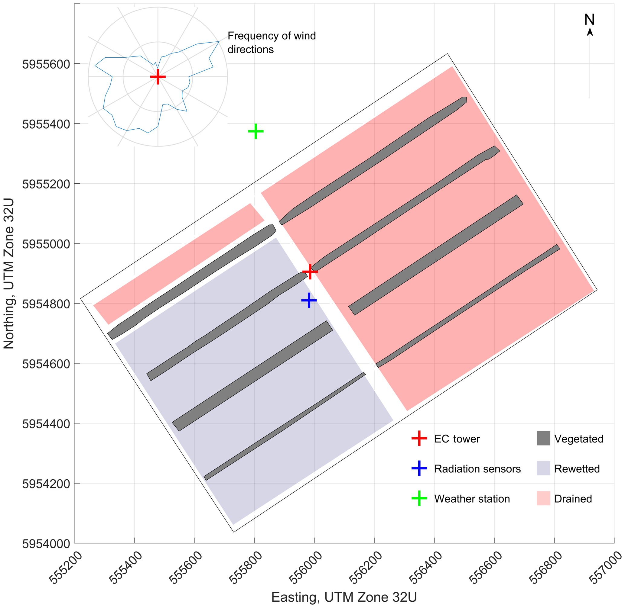
Figure 1 Distribution of surface classes “rewetted”, “drained” and “vegetated” in Himmelmoor during the measurement period between 1 June 2012 and 31 May 2014. The map section shows the central extraction area with the EC tower located on the central railroad dam. Grid spacing is 200 m, coordinates refer to UTM zone 32U. The polar histogram in the top left corner displays 2 years of half-hourly wind direction measurements at the EC tower location binned in 2^∘ classes.

2.1.2 Peat formation and stratigraphy

The bog developed in a river valley, which was preformed as a glacial meltwater valley during the Weichselian glaciation in the depressed fringe of a salt dome. Peatland formation from a standing water body began 10 020±100 years BP (Pfeiffer, 1997). Following the deposition of organic lake sediments, a Phragmites–Carex fen and a subsequent birch forest formed. Around 8000 years BP, a rising groundwater level led to the extinction of the forest vegetation, the spread of Sphagnum spp. peat mosses and eventually the development of a bog. Organic-rich silt constitutes the peatland's foundation but is not evenly distributed across the whole area. In the northern part, this layer is at its thickest (up to 2 m). There, the base of the peatland is at its deepest (around 7 m a.s.l.). The formation of the peatland most likely began at this location (Grube et al., 2010). Bog-type peat consisting mostly of Sphagnum remnants is (in its original stratigraphic position) today only present in the northern marginal area, locally called “Knust”, with a thickness of 3.8 m (Grube et al., 2010). Bog peat was completely removed from the central extraction area where fen-type peat is present area-wide with a maximum thickness of 2.2 m. Pfeiffer (1997) divides these peat deposits in 30–45 cm Eriophorum–Betula peat over 45–85 cm birch forest peat over Phragmites–Carex peat. Soil properties were altered severely by peat decomposition and subsidence during decades of drainage and peat extraction. Drainage led to compaction and settlement of the peat profile of about 40 % of its original depth. The peatland's ability to self-regulate the water table for optimal peat forming and carbon sequestering conditions is thereby lost. The performed ditch-blocking leads to a strongly oscillating water table over the course of the year in the early years of rewetting (<5 years, based on our own observations made between 2011 and 2018). Himmelmoor drains into two local creeks: Bilsbek and Pinnau. The peatland mainly receives water from precipitation. Additional minerotrophic water inflow takes place through the Pütten, which are distributed regularly across the central bog area. These ditches reach below the peat base and penetrate the mineral ground. They were later refilled with peat but still provide a connection to the aquifer beneath, from which minerotrophic groundwater is supplied.

2.1.3 Vegetation

The central, former extraction area is largely vegetation-free. Sphagnum spp. peat mosses occur in ditches and along the shores of some rewetted, inundated polders of the former mining area. Betula pubescens, Molinia caerulea, Eriophorum angustifolium, E. vaginatum, Erica tetralix and brown mosses (Odontoschisma spp., Cephalozia spp.) occur in often isolated patches on drier areas. Fen-type vegetation is common at the Pütten. Betula pubescens, Salix spp. (presumably Salix aurita and Salix caprea), Eriophorum vaginatum, Betula pubescens, Molinia caerulea, Eriophorum angustifolium, Calla palustris, Typha latifolia, Carex spp., Juncus effusus and Calamagrostis canescens occur there. B. pubescens and Salix spp. reached heights of up to 2 m and a combined estimated surface cover within the vegetated strips of up to 10 %.

2.2 Instrumentation

Eddy covariance CH₄ fluxes were measured using an open-path gas analyzer (LI-7700; LI-COR, USA) and a 3D sonic anemometer (R3; Gill, UK) mounted on a tower at 6 m height. Water vapor and CO₂ concentrations were determined with an enclosed-path sensor (LI-7200; LI-COR, USA). Data were recorded on a LI-7550 (LI-COR, USA) logger at 20 Hz. Additionally, a HMP45 (Vaisala, Finland) temperature and relative humidity probe was mounted on the EC tower and logged with the same device. A second HMP45 was installed together with a NR01 four-component net radiometer (Hukseflux, Netherlands), 70 m southwest of the EC tower on a tripod at 2 m height. The radiation sensors were not mounted on the EC tower because the field of view of the downward-facing sensors would have covered the peat dam and would therefore not be representative for a dominant surface type at the site. These data were logged on a CR-3000 (Campbell Scientific, UK). Another logger of this type was used at the weather station, which was taken over from a previous project, and left at a position approximately 500 m north of the EC tower for data consistency. The sensors there included a third HMP45 and a tipping bucket rain gauge (R. M. Young, USA). Per depth, redox potentials were determined with three parallel fiberglass probes with platinum sensor tips and recorded on a Hypnos II logger (MVH Consult, Netherlands). The redox probes were installed in a vegetated strip approximately 100 m west of the EC tower. Water level was measured and logged with a hydrostatic pressure transducer (Mini-Diver; Schlumberger Water Services, USA) around 150 m west-southwest of the EC tower. Rain and long-term temperature data, as presented in Fig. 2, were taken from a nearby station operated by DWD (WMO Station ID 10146), which is located east-southeast from the EC tower at approximately 2 km distance. A total of 2 years of turbulent flux data were available for analysis from Himmelmoor. The EC setup did not change during that time. The first year from 1 June 2012 to 31 May 2013 is from hereon called Year 1, the second year from 1 June 2013 to 31 May 2014 is called Year 2.

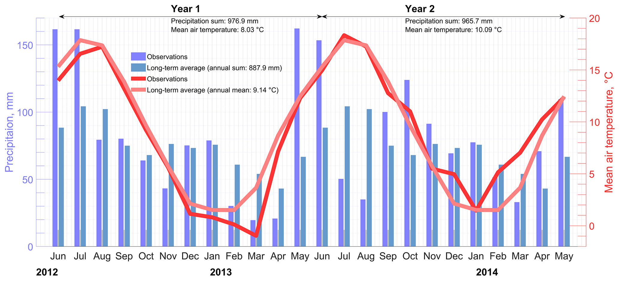
Figure 2 Climate diagram of the 2 investigated years from 1 June 2012 to 31 May 2013 (Year 1) and from 1 June 2013 to 31 May 2014 (Year 2) as measured in Himmelmoor and a 14-year average of a nearby DWD station (WMO Station ID 10146).

2.3 Flux calculation and quality filtering

Turbulent fluxes were computed by applying the EC approach (as, for example, described in more detail by Aubinet et al., 2012) using the software EddyPro 5.2.1 (LI-COR, USA). Raw data processing included (1) an angle of attack correction, i.e., compensation for flow distortion induced by the anemometer frame (Nakai et al., 2006); (2) coordinate rotation to align the anemometer x axis to the current mean streamlines (Kaimal and Finnigan, 1994, double rotation); (3) linear detrending (Gash and Culf, 1996); (4) time lag compensation; (5) spectral corrections (see below for details); and (6)  Webb–Pearman–Leuning (WPL) correction to compensate for air density fluctuations, due to thermal expansion and water dilution (Burba et al., 2012). High-frequency loss due to path averaging, signal attenuation and the finite time response of the instruments was accounted for following Fratini et al. (2012). Low-frequency loss due to finite averaging time and linear raw data detrending was corrected for according to Moncrieff et al. (2004). More details on the single flux calculation steps are given in Holl et al. (2019a). Several 30 min fluxes were screened for quality according to the following scheme. To check whether general assumptions necessary for the application of the EC method were met, atmospheric stability and developed turbulence were analyzed as described by Mauder and Foken (2004). By this step, fluxes were classified into three groups: MF0, MF1 and MF2, with MF0 denoting data of the highest quality and MF2 denoting that of the lowest quality. Due to potentially faulty WPL correction, CH₄ and CO₂ fluxes of increments of 30 min when sensible (H) or latent (LE) heat flux were flagged with MF2 were discarded. Certain quality flags that were derived from raw data statistics as described by Vickers and Mahrt (1997) were evaluated. If skewness or kurtosis of vertical wind or sonic temperature were assigned a hard flag (skewness outside [−2, 2] and kurtosis outside [1, 8]) or if CH₄ or CO₂ concentration statistics were rated with a soft flag (skewness outside [−1, 1] and kurtosis outside [2, 5]), trace gas fluxes where discarded. Furthermore, half-hourly fluxes were rejected if the respective 20 Hz concentration time series failed the amplitude resolution test (Vickers and Mahrt, 1997).

Additionally, diagnostic values from the LI-7700 and LI-7200 gas analyzers were used for quality screening. LI-7200 data were omitted when the signal strength indication (AGC) lay above 63. Due to a change in the signal quality definition along with a software upgrade, this rule was modified to discard data below a value of 75 for data acquired when the sensor was running on firmware version 6.6 and above. With respect to the LI-7700, the sensor's relative signal strength indication (RSSI) and the heater diagnostics were evaluated. The bottom and top mirror of the gas analyzer's measurement cell can be heated to counter condensation and frost on the mirrors. The LI-7700 instrument software allows for user-defined thresholds that control the powering on of the heaters. For the bottom heater, a RSSI threshold RSSI_th, below which the heater is turned on, can be adjusted. For the top heater, an ambient temperature offset threshold T_a,offset can be defined. This mirror is heated to keep its temperature about T_a,offset above ambient temperature. In the present case, RSSI_th was set to 20 and T_a,offset to 1^∘ C. The number of samples within 30 min, for which a heater is switched on, is recorded. Accordingly, these diagnostics (bottom heater on: BH_on; top heater on: TH_on) take maximum values of 36 000 if a heater is switched on for 30 min. Heater diagnostics were investigated closely due to the observation that, within an averaging interval, high variation in RSSI was often accompanied by switching events in the 20 Hz heater time series, i.e., if BH_on or TH_on were neither 0 nor 36 000. Moreover, methane concentrations had the tendency to covary with RSSI values if the latter showed large changes, which renders calculated fluxes not trustworthy. In general, the top heater was switched on most of the time, whereas switching events in the BH_on time series were more common, which is why we mainly focused on the bottom heater diagnostics for the analysis of this phenomenon. Figure 3 shows the relationship between half-hourly averaged RSSI values, the corresponding relative standard deviation of 20 Hz RSSI (RSSI_relStd) values and BH_on. From this graph, we empirically derived a RSSI_relStd threshold of 10 %, above which the respective flux records were neglected. Additionally, methane fluxes were discarded if the mean RSSI of the respective averaging interval was below 20.

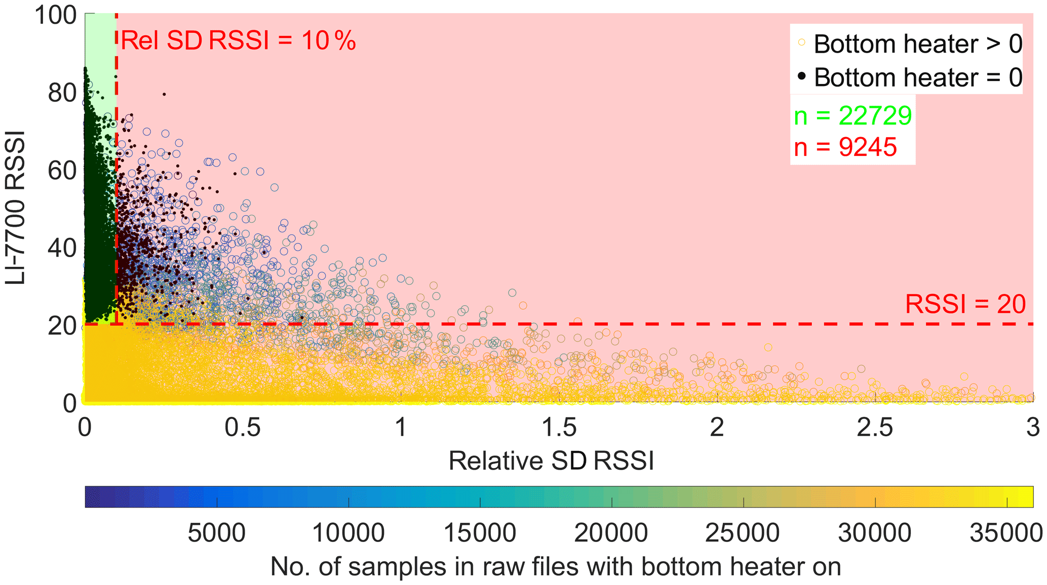
Figure 3 Illustration of the empirically derived threshold for the new LI-7700 open-path methane analyzer quality filter. This check evaluates raw 20 Hz RSSI statistics to remove erroneous half-hourly methane fluxes. The filter is designed to capture concentration time series that were deteriorated by switching events in a LI-7700 mirror heater. Black data points denote 30 min intervals, during which the heater of the bottom mirror was switched off entirely. Colored points represent 30 min intervals, during which switching events (maximum: 36 000) in the 20 Hz time series occurred.

The next quality-screening step addressed the filtering of fluxes related to undesired source areas. We first classified the surface using georeferenced orthoimages of the area. As the surface types we aimed to discriminate were quite large and easily distinguishable in the images, we could draw polygons around the different classes and get the coordinates of their corners. This step was implemented through the MATLAB 8.4 Mapping and Image Processing Toolboxes. We defined the surface classes as drained (SC_dra), rewetted (SC_rew) and vegetated (SC_veg), the latter of which is contained in the other two surface types as formerly deep, now refilled and vegetated ditches (Pütten). Calculating a 2D footprint function after Kormann and Meixner (2001) with 1 m² resolution (see Holl et al., 2019b, for details on footprint model implementation) and summing up the contribution values of all pixels within each of the three surface types, yielded half-hourly class contribution fractions of the different classes to the EC signal (CC_rew; CC_dra; CC_veg). Variations in vegetation height and thereby roughness length in different wind sectors were addressed by statistically determining roughness length estimates separately for 2^∘ wind sectors prior to evaluating the footprint model (see Holl et al., 2019b, for details). Gas fluxes of 30 min intervals, when the EC footprint was composed of the railroad dam and areas outside the mining site by more than 70 %, were discarded. Fluxes were then filtered for absolute limits. CH₄ data outside [−100 1000] nmol m⁻² s⁻¹ and CO₂ data outside [−10 10] µmol m⁻² s⁻¹ were neglected. In the case of the CH₄ flux time series, outlier removal was addressed furthermore by assessing the frequency distribution of the remaining MF0 data. Values smaller than the bin center of the 1st percentile (BC₁) or larger than the 99th percentile's bin center (BC₉₉) were omitted. As a last step, CH₄ fluxes with random uncertainties calculated with EddyPro following Finkelstein and Sims (2001) larger than 400 nmol m⁻² s⁻¹ were filtered out.

Overall, a large amount of data were removed throughout the course of quality filtering. Of the original 19 665 $F_{{\mathrm{CH}}_{\mathrm{4}}}$ records, 28 % of quality classes MF0 and MF1 were left after filtering. Most fluxes (35 %) were removed because they failed the skewness–kurtosis test. In the case of CO₂ fluxes, 51 % of MF0 and MF1 records of the original 31 271 fluxes remained after filtering. The largest amount of data (15 %) were removed because either H or LE of the same 30 min interval were flagged with MF2.

2.4 Flux modeling

We applied a two-step gap-filling process to CO₂ and CH₄ fluxes separately for each of the 2 available years. We first filled gaps resulting from quality filtering of the measured EC gas fluxes, which represent approximations of the landscape-scale fluxes integrated over the whole ecosystem and thus include areas of contrasting land use types (tower view time series, TVTS). In order to quantify the impact of rewetting on the vertical annual C balances of the peat extraction areas in Himmelmoor, we used EC footprint variables to select fluxes when the EC source area was mainly composed of drained or rewetted surfaces, respectively. In particular, we created these surface class time series (SCTS) by selecting all flux values for the class contributions CC_dra and CC_rew above a threshold of 70 %. As this data division necessarily resulted in further gaps in the SCTS, we used new sets of models to fill those gaps. We used multilinear regressions (MLRs) and artificial neural networks (ANNs), in particular multilayer perceptrons (MLPs), to model gas fluxes as a response to measured environmental and EC footprint variables and to generate fuzzy logic representations of diurnal and seasonal periodicity. Additionally, we used a model input selection scheme in an effort to exclude redundant and irrelevant variables from the model input matrix. A description of model input selection and model setup is given in the Supplement to this article. Details on data set division by surface class contribution, gap-filling and flux decomposition are given here.

Apart from the class contribution variables, the inputs presented to the selection scheme were the same for TVTS and SCTS modeling. To gap-fill a SCTS, the contributions of the respective opposite surface classes were omitted from the input space. To model the time series representing the rewetted area for instance, CC_dra and CC_veg,dra (see Table A1) were removed from the input matrix. Also, the surface class of interest was set to the threshold value of 70 % at all flux gaps that resulted from data division. We used this threshold value instead of 100 % class contribution to avoid extrapolating outside the scope of the training data sets, as the EC footprint was virtually never composed of one surface class only. The measured contributions of the vegetated strips were binned in 10 classes and the bin center of the most frequent class was used to fill gaps in the respective CC_veg time series.

We used the selected variables as inputs for MLRs and MLP ensembles with 1000 networks each. To optimize the model parameters, we used only observed data of quality class 0 as targets. Based on the better performance of MLPs compared to MLRs (see Sect. 3.2), we decided to use MLP models for TVTS and SCTS gap-filling. To express model uncertainty, we used the standard deviations of the 1000 single MLPs making up each model ensemble for each increment of 30 min. We confirmed normal distribution of the 1000 model fluxes for each 30 min interval by applying a Kolmogorov–Smirnov test at all time steps. To calculate surface-class-specific annual sums, we included measurement data of quality class 1 back into the SCTS. All quality class 1 values that corresponded to CC_dra or CC_rew ranging above 70 % were used to replace the modeled SCTS data for the respective time steps. We filled remaining gaps in the gas flux time series, when no environmental data were available, with a mean diurnal variation (MDV) method (see Falge et al., 2001). If this algorithm encounters a gap, it searches for available values of the same variable in adjacent days at the same hour of the day and uses the mean of the found records to fill the gap. At first, a window of ±1 d around the gap is screened. If at least one data point is not found, the search range is increased in steps of 1 d until the gap can be filled. We calculated two annual sums for all four SCTS (two gases and two land use types) from the gap-filled time series. We calculated uncertainty estimates of the annual sums by taking the root of the sum of squared half-hourly uncertainties. For measurements we used the random uncertainty estimate following Finkelstein and Sims (2001), for data modeled with an MLP ensemble we used the ensemble standard deviation and for data modeled with the MDV method we used the standard deviation of averaging samples.

In the case of the $F_{{\mathrm{CO}}_{\mathrm{2}}}$ SCTS, we used a deterministic modeling approach to further decompose the net flux into components related to respiration and photosynthesis. As large parts of Himmelmoor are vegetation-free, we included the class contribution of the vegetated strips (Pütten, SC_veg) to the EC footprint to scale the model terms relating to the respective surface classes (as in, e.g., Rößger et al., 2019; Forbrich et al., 2011) in the following way:

$$\begin{array}{}\text{(1)}& \begin{array}{rl}\mathrm{NEE}& ({\mathrm{CC}}_{\mathrm{veg}},\mathrm{PAR})=(\mathrm{1}-{\mathrm{CC}}_{\mathrm{veg}})\times {\mathrm{TER}}_{\mathrm{bare}}+{\mathrm{CC}}_{\mathrm{veg}}\\ & \times {\mathrm{TER}}_{\mathrm{veg}}-{\mathrm{CC}}_{\mathrm{veg}}\times {\displaystyle \frac{P_{\max }\times \mathit{\alpha }\times \mathrm{PAR}}{P_{\max }+\mathit{\alpha }\times \mathrm{PAR}}},\end{array}\end{array}$$

where NEE is the net ecosystem exchange of CO₂ (µmol m⁻² s⁻¹); CC_veg is the class contribution of the vegetated strips; PAR is photosynthetically active radiation (µmol m⁻² s⁻¹); TER_veg and TER_bare are ecosystem respirations (µmol m⁻² s⁻¹) of the vegetated strips and the areas covered by bare peat, respectively; P_max is the maximum photosynthetic rate (µmol m⁻² s⁻¹); and α is the initial quantum yield. Prior to fitting, CC_veg and CC_bare were rescaled to sum up to 1 so that

$$\begin{array}{}\text{(2)}& \mathrm{1}-{\mathrm{CC}}_{\mathrm{veg}}={\mathrm{CC}}_{\mathrm{bare}}.\end{array}$$

The last term of Eq. (1) consists of a rectangular hyperbolic Michaelis–Menten type function to simulate plant photosynthesis (Thornley, 1998; Zheng et al., 2012). This type of light saturation curve has proven to be feasible for modeling plant carbon dioxide fixation driven by radiation. In order for the model to express net CO₂ flux, two ecosystem respiration terms were added to the formula: the combined plant and soil respiration TER_veg scaled by CC_veg and the microbial respiration TER_bare taking place in the vegetation-free areas scaled with CC_bare. This function was fitted to monthly ensembles of all CO₂ SCTS, yielding time series of the four model parameters for the drained and rewetted areas for 2 years. The included scaling of the model terms with the surface class contributions facilitates comparability of the parameter time series among each other and with literature values describing the light response of similar plant communities as found in the vegetated strips of Himmelmoor.

3 Results and discussion

3.1 Model input selection and flux–driver relations

Detailed results of our model input selection scheme are given in the Supplement to this article. A summarized description follows here. Three categories of potential model inputs were presented to the selection scheme: 30 min time series of meteorological and soil (Biomet) variables, fuzzy variables representing diurnal and seasonal cycles (following Papale and Valentini, 2003) and footprint variables in the form of surface class contribution estimates. Table A1 gives an overview of the available variables. Note that in Year 1 no soil properties were recorded.

In the case of CO₂ flux modeling, all input matrices contain measures for the main driver of photosynthesis, which is radiation. PAR and R_g were selected for both land use types in Year 1 and the time-lagged version of PAR for both land use types in Year 2. More emphasis on the impact of plant activity on CO₂ fluxes is shown by the inclusion of the footprint contribution of the vegetated strips for both years and land use types. A response of CO₂ release to respiration is indicated by the selection of peat temperatures, redox potentials and water table height in Year 2 and Lw_out in Year 1. T_air was selected for all land use types and years and includes both seasonal and diurnal frequency content like the slowly and quickly changing fuzzy variables which belong to all final input spaces as well.

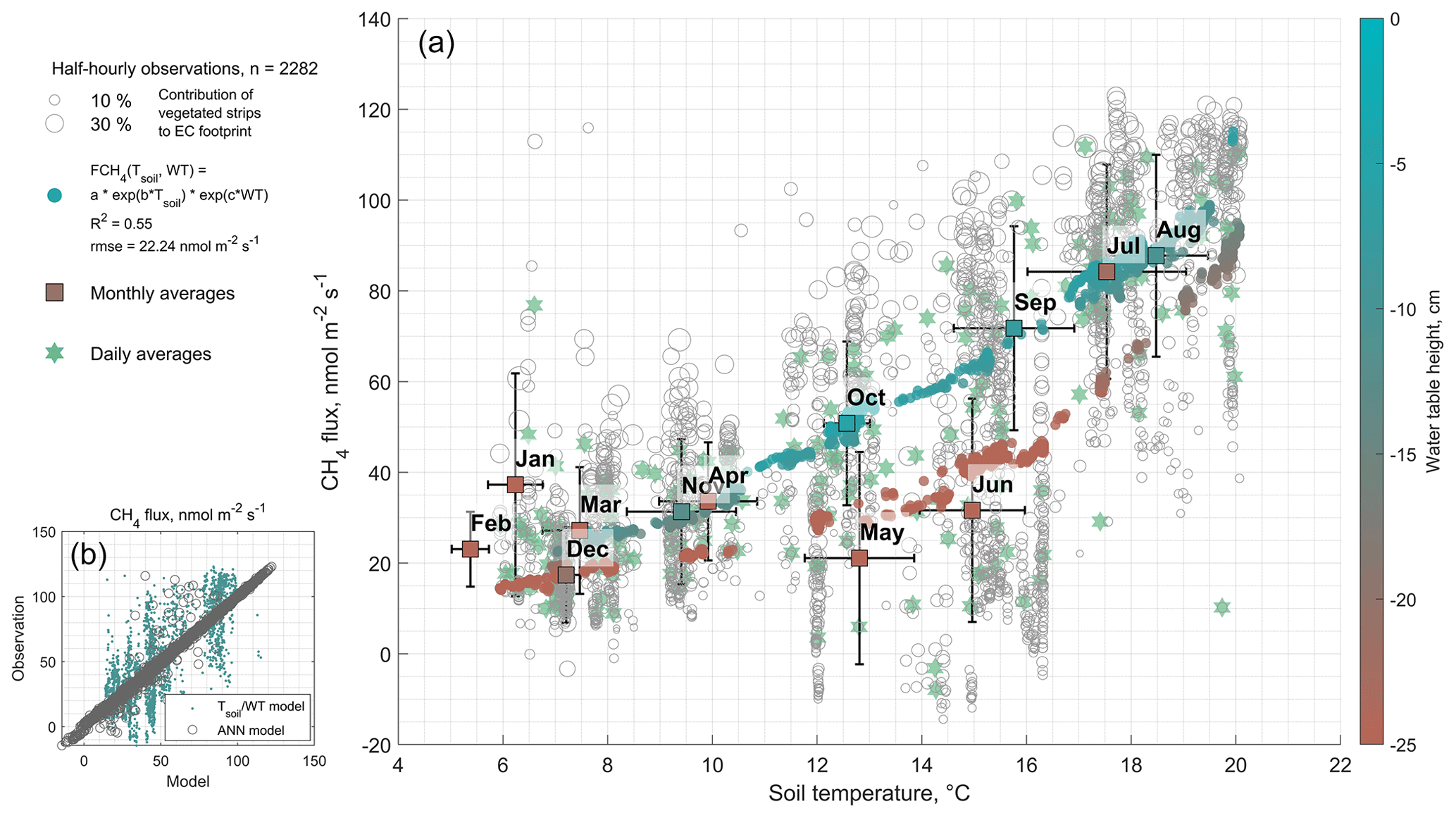
Figure 4 (a) Observed half-hourly methane fluxes ($F_{{\mathrm{CH}}_{\mathrm{4}}}$) from the rewetted section of Himmelmoor modeled as an exponential function $F_{{\mathrm{CH}}_{\mathrm{4}}}$ (T_soil, WT) of soil temperature at 40 cm depth (T_soil) and the water table (WT). Monthly and daily flux and temperature averages are also given. (b) Comparison of a more complex artificial neural network (ANN) model with the exponential model from (a). Although methane flux variability can be explained by the exponential model to a reasonable degree, the level of complexity in flux–driver relations appears to be considerably better represented by the ANN.

In the case of CH₄ flux modeling, the selection scheme focused on the footprint contribution of the vegetated strips, water vapor pressure deficit (VPD, Pa) and peat temperatures in both years and for both land use types. In Year 1, soil temperatures were indirectly addressed by the inclusion of Lw_out (being a measure of surface temperature) and fuzzy_su, which is correlated strongly to T_Soil40 (Pearson's correlation coefficient r=0.9). Diurnal and seasonal cycles were weighted highly by the inclusion of higher-frequency fuzzy variables, VPD and T_air in both years. In Year 1, p_air was included for the rewetted section, stressing the higher likelihood of ebullition events taking place at these inundated areas, which could be facilitated by air pressure variations. The selection of redox potential and water table height time series in Year 2 gives further confidence that our scheme is able to identify physically meaningful driving variables, as soil redox conditions are known to be a major limiting factor for methane production in soils.

To further investigate the relation between CH₄ flux and likely drivers as identified by our model input selection scheme, we fitted an exponential model of water table and soil temperature (in 40 cm depth) to the CH₄ fluxes from the rewetted section (see Fig. 4). With the exponential dependence of $F_{{\mathrm{CH}}_{\mathrm{4}}}$ on soil temperature, a fair amount (R²=0.55) of the flux variability can be explained while the added water table term allows for the optimized temperature–$F_{{\mathrm{CH}}_{\mathrm{4}}}$ curve to take two distinct paths above and below an approximate water table threshold of 20 cm below the surface (see Fig. 4a). Half-hourly flux variability is, however, substantial due to the heterogeneity of the site's surface and other confounding factors like the above-mentioned air pressure variations and is comparably better explained by our neural network models (see Fig. 4b).

3.2 Model performance

In order to (i) evaluate the general feasibility of our flux decomposition and modeling method and to (ii) compare the performance of MLP and MLR models, we used four approaches. We first compared statistics of MLP and MLR surface-class-specific flux models with observed data, which we separated beforehand using an EC footprint model into fluxes relating to either one of the two main surface classes SC_dra and SC_rew. Results are shown in Figs. B1 and B2 in the Appendix B. In all eight cases (2 years, two gases, two surface classes), MLPs outperform MLR models with respect to coefficient of determination (R²), Akaike information criterion (AIC) values and root-mean-squared error (RMSE). While MLRs often perform well, there is a tendency for them to overestimate the highest and underestimate the lowest fluxes in the case of CH₄ flux modeling, leading to S-shaped point clouds around the 1:1 line in the scatterplots given in Fig. B1. In the case of CO₂ models, this tendency of MLRs appears to be less pronounced, whereas there is one case (Year 1, SC_dra; see Fig. B1) where the MLR model explains only 32 % of the measurement data's variability and is therefore evaluated as inept for gap-filling of at least this data set. As a way to evaluate the generalization capability of both model types independently from data used for model optimization, we secondly drove the models, which were optimized using Year 1 observations with Year 2 environmental data, and compared the results to Year 2 measurements (see Fig. 5). Results highlight the applicability of both model types for gas flux time series extrapolation, while MLPs again perform better compared to MLRs in all cases. As expressed in the lower AIC values throughout, the higher model complexity of the MLPs appears to be justified, and the better goodness of fit measures do not seem to be the result of a too tight approximation of the training data. We attribute this result partly to our efforts to reduce the number of hidden layer nodes and the number of independent input variables (i.e., dimensionality reduction of the model input matrices). As a third way to compare model performance and evaluate our method of decomposing gas flux time series obtained with a single EC tower over heterogeneous terrain into surface-class-specific time series, we recombined these SCTS by scaling them with their respective contribution to the EC footprint. We calculated the sum of both scaled half-hourly SCTS and compared them to the TVTS measured over heterogeneous terrain at the EC tower. These fluxes also include values with mixed surface class contributions below the threshold of 70 %, which was used to extract target data for SCTS model optimization. Results are shown in Fig. 6 and again illustrate the better performance of MLPs compared to MLRs. More importantly, the outcome of this circular rescaling experiment demonstrates that after multiple model layers the original measurement data relating to a heterogeneous surface could still be recovered to a reasonable degree.

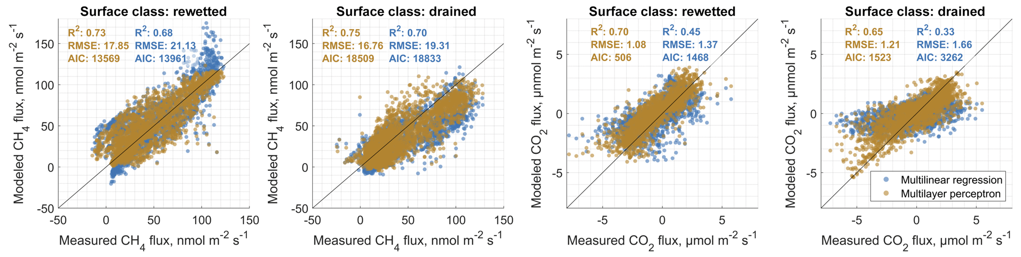
Figure 5 Comparative validation of surface-class-specific multilinear regression and artificial neural network (in particular multilayer perceptron) carbon dioxide (CO₂) and methane (CH₄) flux models. For this depiction, we drove models that were optimized using Year 1 measurement data as targets with Year 2 environmental data and compared the results to measured Year 2 gas fluxes. This type of comparison enables an evaluation of the developed models with observed data that are completely independent of model optimization. Therefore, good agreement cannot be attributed to models that are overfit to the provided target data. The results of this investigation substantiate the notion that multilayer perceptrons provide more reliable estimates of gas fluxes, as they are superior to multilinear models with respect to the coefficient of determination (R²), the Akaike information criterion (AIC) and the root-mean-squared error (RMSE) in all cases.

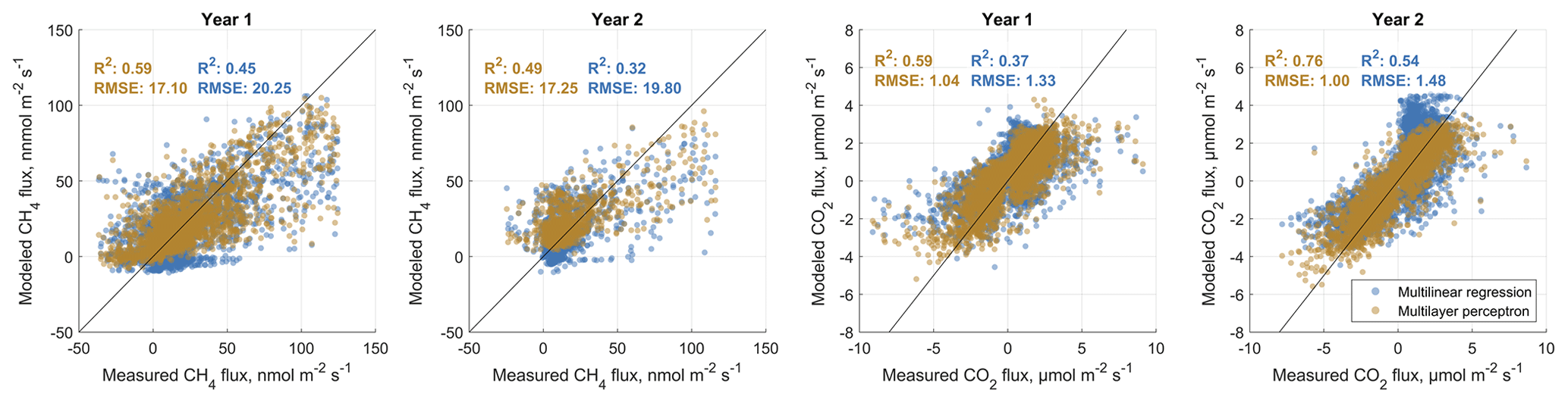
Figure 6 Comparative validation of multilinear regression and artificial neural network (in particular multilayer perceptron) carbon dioxide (CO₂) and methane (CH₄) flux models. For this analysis, both surface-class-specific flux models were combined using the footprint contribution of the respective classes, yielding an estimate of the landscape-integrated signal recorded at the eddy covariance tower. These derived “tower view” gas flux time series are compared to the actually observed data at the eddy covariance tower. In all cases, the multilayer perceptron models' performances surpass the attainment of multilinear regression models with respect to the coefficient of determination (R²) and the root-mean-squared error (RMSE). Results also highlight the general feasibility of our approach to decompose an eddy covariance (EC) time series recorded over heterogeneous terrain into contributions of differently functioning landscape units within the EC footprint area.

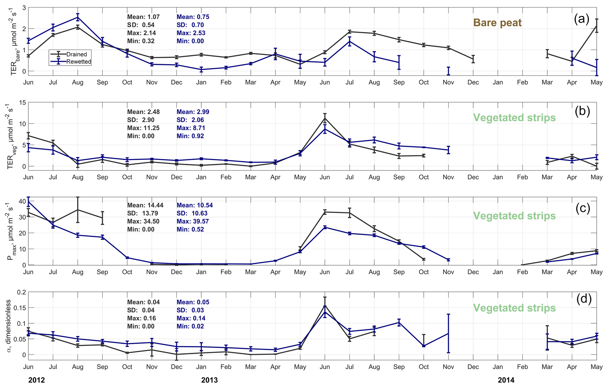
Figure 7 Time series of monthly carbon dioxide flux model parameters (see Eq. 1). Total ecosystem respiration (TER) series are given for the bare (a) and vegetated (b) sections of Himmelmoor. The photosynthesis parameters of maximum photosynthesis P_max (c) and initial quantum yield α (d) were only determined for areas with vegetation. All parameter time series are given for the rewetted and drained sections of Himmelmoor.

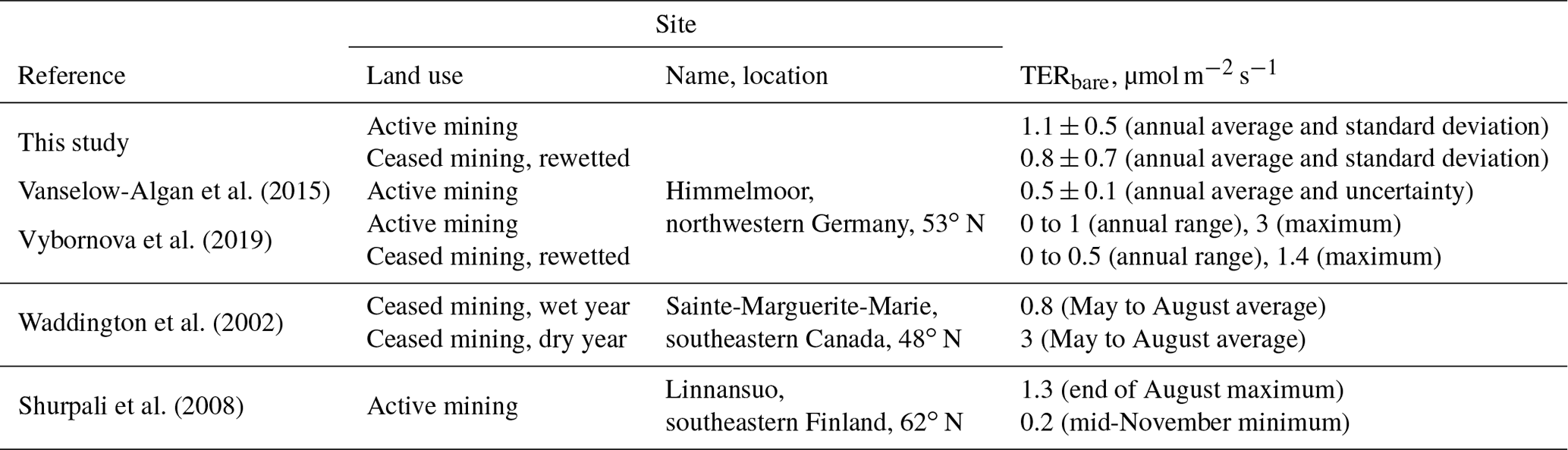
As a fourth method to evaluate the applicability of our land-use-specific flux decomposition, we fitted a combined respiration–photosynthesis model (see Eq. 1) to monthly ensembles of the half-hourly CO₂ SCTS in order to check if the resultant parameters are reasonable in relation to each other and to literature data. In general, the vegetation period, with its productivity maximum between June and July and its cessation between mid-October and November is depicted well in the seasonal course of the model parameters throughout both years. The parameter courses relating to the vegetated strips of the drained and rewetted areas (Fig. 7b–d) develop in a fairly similar way. Distinctions between the drained and rewetted areas are more pronounced with respect to CO₂ release from bare peat surfaces (Fig. 7a). Ditch-blocking of a rewetted sector close to the EC tower (which therefore made up a large part of the EC footprint) was only performed 1 year before our measurements started. Therefore, in the summer of 2012 this area was not yet permanently flooded, leading to TER_bare fluxes exceeding those from the active mining site. From winter 2012/2013 on, inundation of the rewetted bare peat area progressively increased, resulting in lower TER_bare fluxes from the rewetted section compared to the drained section. Our TER_bare fluxes are in concordance with findings from two studies that were also conducted on the active peat extraction area in Himmelmoor with manual chambers; TER data reported from similar peat extraction sites also agree with our results (see Table C2).

As our model includes the relative contributions of the vegetated strips to the EC footprint, we compared the extracted model parameter time series (see Fig. 7b–d) with estimates of these plant-species-specific values from other studies investigating similar plants and plant communities as found in the vegetated strips in Himmelmoor. Reported averages and ranges agree with our findings well (see Table C1). Additionally, we could distinguish between CO₂ release from decomposing bare peat (TER_bare; see Fig. 7a and Table C2) and from the vegetated strips (TER_veg; see Fig. 7b and Table C1) where respiratory CO₂ release also includes autotrophic respiration of plants. In our data set, TER is between 2-fold and 4-fold larger in areas with vegetation than without vegetation. TER_veg from the rewetted area is mostly larger than that from the drained area. Progressive inundation led to a hydrological connection of SC_veg and the flooded bare peat areas. An increased input of dead plant material as a result of higher water tables might have promoted heterotrophic respiration. Hampered plant productivity due to flooding is also expressed in lower peak values of P_max at the vegetated strips of the rewetted site.

In comparison to small-scale measurements from the same and similar sites, we could confirm the credibility of our mechanistic modeling approach for which we used relative class contributions of contrasting surface types to scale single model terms. Moreover, the previously performed division of the TVTS into SCTS apparently yields reasonable flux estimates that can be interpreted in a mechanistic way, increasing our confidence in the applied flux decomposition method.

3.3 Annual greenhouse gas balances

We used the eight (two gases, two land use types, 2 years) surface-class-specific flux time series, which we gap-filled with MLP ensembles, to calculate annual CO₂ and CH₄ balances for the rewetted and drained sections of Himmelmoor.

Table 1 Annual sums of half-hourly carbon dioxide (CO₂) and methane (CH₄) fluxes from the drained and rewetted sections of the peat extraction site in Himmelmoor. CH₄ fluxes are expressed as CO₂ equivalents (CO₂ eq.) using a global warming potential of 34, referring to a 100-year time horizon following Myhre et al. (2013). Year 1 is 1 June 2012 to 31 May 2013, and Year 2 is 1 June 2013 to 31 May 2014.

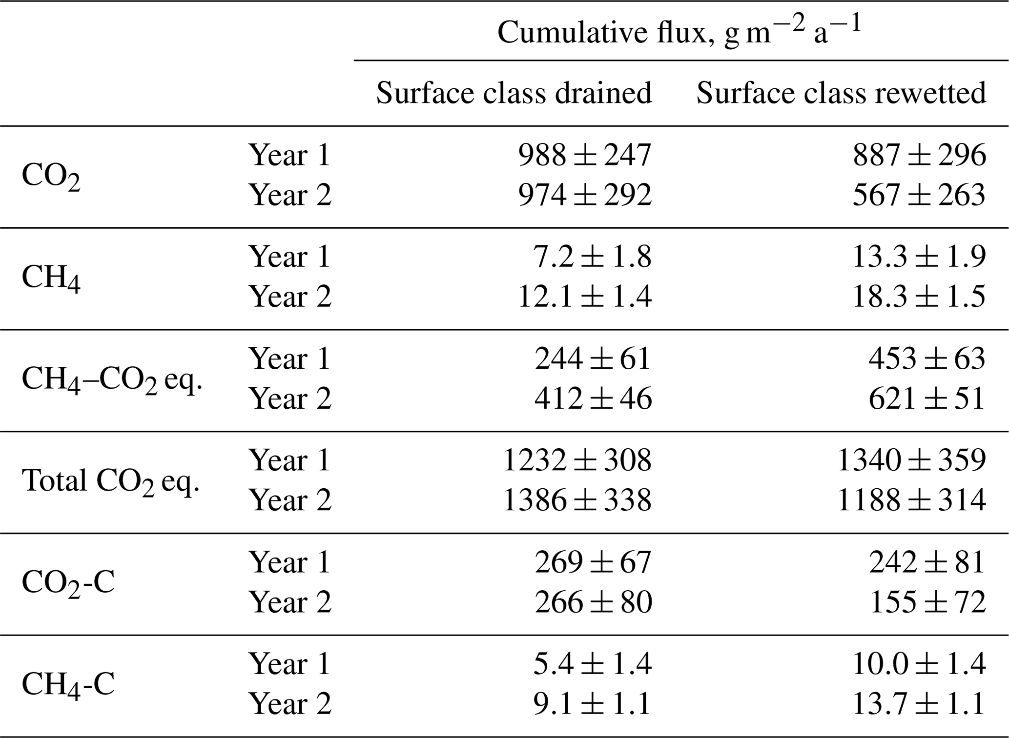
The results are expressed as molar and mass fluxes (Fig. 8) and as release of CO₂ equivalents (CO₂ eq.; see Table 1). We used a factor of 34 to convert $F_{{\mathrm{CH}}_{\mathrm{4}}}$ into CO₂ eq. release. This value is given in the Fifth Assessment Report of the Intergovernmental Panel on Climate Change (IPPC AR5, Myhre et al., 2013), refers to a 100-year time horizon and includes climate–carbon feedbacks. The impact of rewetting on the development of vertical carbon release is documented with the shown results. Overall, both the rewetted and the mined sections of Himmelmoor were considerable sources of GHGs in both years. Annual $F_{{\mathrm{CO}}_{\mathrm{2}}}$ from the restored site undercuts the cumulative CO₂ emissions from the drained part of Himmelmoor in both years, while this difference increases with time. Annual CH₄ release from the wetter surfaces exceeds the cumulative $F_{{\mathrm{CH}}_{\mathrm{4}}}$ from the drained mining site in both years, while both fluxes rise from Year 1 to Year 2.

In Year 1, $F_{{\mathrm{CO}}_{\mathrm{2}}}$ from the rewetted area was already cumulatively lower than from the mining site (20±7 vs. 22±6 mol m⁻² a⁻¹), while the margins of uncertainty largely overlap. In Year 2, the annual CO₂ balance from the rewetted site dropped by 35 % increasing the difference to the cumulative mining site flux, which did not change from Year 1 to Year 2, to over 40 % (13±6 vs. 22±7 mol m⁻² a⁻¹). Margins of uncertainty still overlap in Year 2 but less widely. At the end and the beginning of Year 2 (i.e., in summer), the cumulative $F_{{\mathrm{CO}}_{\mathrm{2}}}$ curve from SC_rew ceases to slope upwards. By reaching these vertexes, the points in time when the rewetted area briefly turns from a CO₂ source into a sink are indicated. Nevertheless, annually integrated ecosystem respiration outweighs photosynthesis in SC_rew.

CH₄ fluxes from both surface classes rise from Year 1 to Year 2, while the absolute differences between both land use types stay rather constant. The cumulative CH₄ flux from SC_rew is nearly 90 % higher than from SC_dra in Year 1 (0.45±0.11 vs. 0.83±0.12 mol m⁻²) and 50 % higher in Year 2 (0.76±0.08 vs. 1.14±0.09 mol m⁻²). Compared to the molar $F_{{\mathrm{CO}}_{\mathrm{2}}}$ sums of both surface classes, cumulative molar CH₄ release is around a factor of 30 smaller in Year 1 and about 20 times smaller in Year 2. The development of both molar GHG emissions over time documents the rising importance of CH₄ emissions in the course of rewetting. Transforming the molar cumulative sums into sums of CO₂ eq. allows for comparability between the two GHG fluxes with respect to their climate impact. Overall, the rewetted section of Himmelmoor is a larger CO₂ eq. source in the first observed year, while the drained section emits more CO₂ eq. in Year 2. CO₂ eq. fluxes at the drained site increase from Year 1 to Year 2, whereas they decline from Year 1 to Year 2 at the rewetted site. The sum of cumulative $F_{{\mathrm{CO}}_{\mathrm{2}}}$ and $F_{{\mathrm{CH}}_{\mathrm{4}}}$ released from SC_dra are dominated by $F_{{\mathrm{CO}}_{\mathrm{2}}}$ in both years. For SC_rew, CH₄–CO₂ eq. emission sums are much smaller than the release of CO₂ in Year 1, whereas CH₄–CO₂ eq. fluxes dominate the GWP balance in the second observed year. Although the cumulative CH₄–CO₂ eq. fluxes also increase from Year 1 to Year 2, they mainly dominate the SC_rew GWP sum due to a large drop in $F_{{\mathrm{CO}}_{\mathrm{2}}}$ from Year 1 to Year 2.

The annual CO₂ emissions from the drained parts of 988±247 and 974±292 g m⁻² a⁻¹ are higher but in the same range as previously inferred from chamber data acquired at the mining site in Himmelmoor by Vanselow-Algan et al. (2015) (730±67 g m⁻² a⁻¹) and Vybornova et al. (2019) (740±270 g m⁻² a⁻¹). Moreover, our results are in line with the emission factors given in the Wetlands Supplement to the 2006 IPCC Guidelines for National Greenhouse Gas Inventories (Hiraishi et al., 2014), for which Wilson et al. (2016a) published an update. Both publications give an average CO₂ release of 1027 g m⁻² a⁻¹ for boreal and temperate peatlands drained for peat extraction. While boreal extraction sites generally appear to emit less CO₂, as reported in a meta-study by Maljanen et al. (2010) (697±263 g m⁻² a⁻¹), Drösler et al. (2008), who analyzed 11 drained peat extraction sites in Europe, also report CO₂ release of up to 1300 g m⁻²a⁻¹. Interesting to note is that in the National Inventory Report Germany submitted under the United Nations Framework Convention on Climate Change in April 2019, CO₂ release from drained peat extraction areas are accounted for with a comparably small factor of 587 g m⁻² a⁻¹. Taking into account the amount of carbon removed from Himmelmoor by peat extraction (11 000±1000 g m⁻² a⁻¹), CO₂ emissions account for less than a tenth of the total carbon loss per year. This value from Vanselow-Algan et al. (2015) is, however, expressed as CO₂ and assumes the instant decomposition of the material after removal. Restored cutover bogs commonly are CO₂ sinks when active peat extraction has been ceased for several decades (Tuittila et al., 1999; Wilson et al., 2016b; Beyer and Höper, 2015). However, shortly after ditch-blocking, the rewetted section of Himmelmoor was still a considerable CO₂ source (887±296 and 567±263 g m⁻² a⁻¹). During regular visits to the area between 2011 and 2019, we observed that the amplitude of seasonal water table oscillations in a rewetted, formerly mined strip (polder) would decrease with the time passed after ditch-blocking. We assume that anoxic conditions did not prevail throughout the year in all polders as already discussed above with respect to TER_bare fluxes from these sites. Additionally, ditch-blocking in Himmelmoor went along with the construction of dams encompassing the newly rewetted polders. Vybornova et al. (2019) showed that shortly after raising these dams they can be large sources of CO₂ with fluxes up to 4 times larger than from bare peat areas which are drained for ongoing mining.

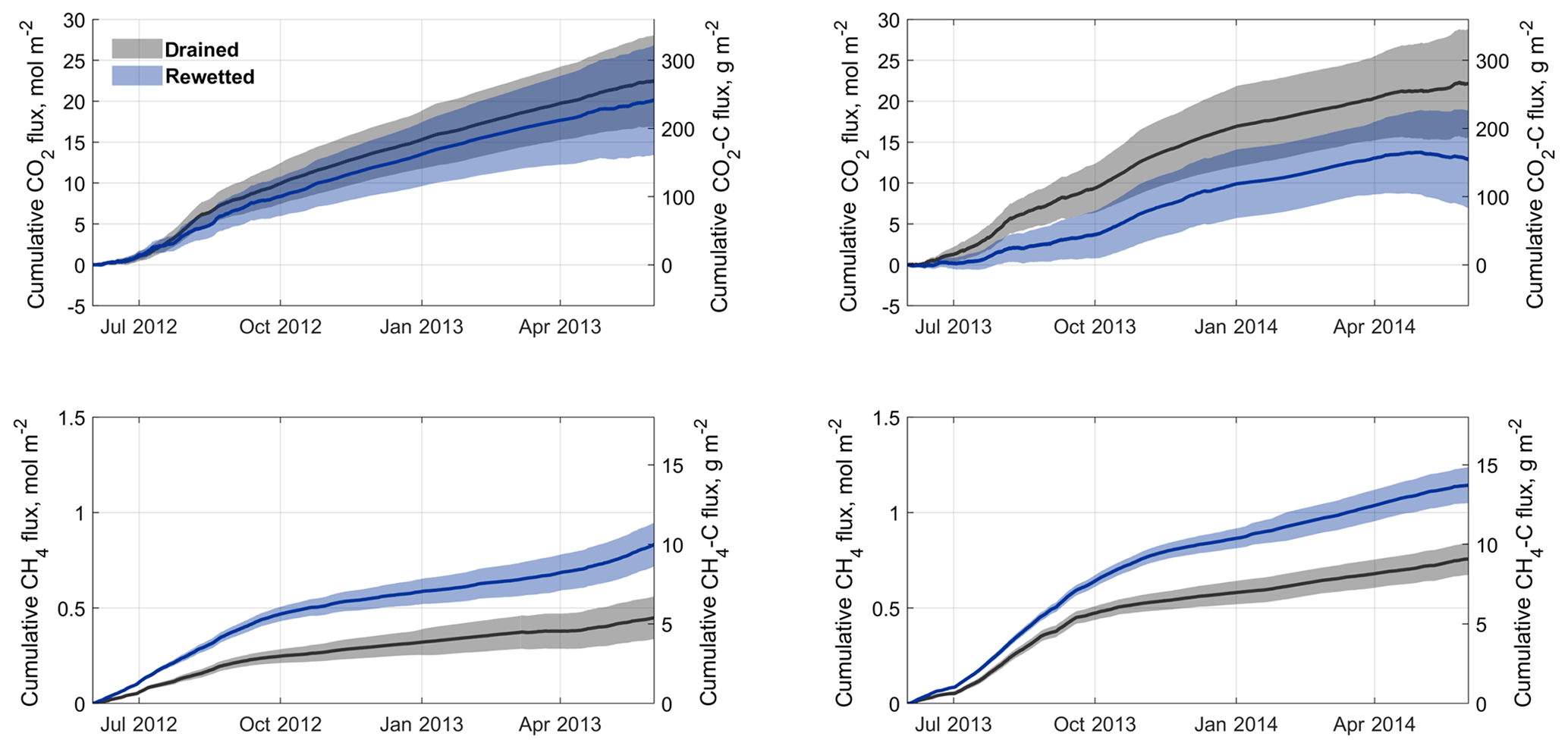
Figure 8 Cumulative carbon dioxide (CO₂) and methane (CH₄) fluxes from the drained and rewetted sections of the peat extraction sites in Himmelmoor for both investigated years. Shaded areas represent model uncertainty estimates derived from the standard deviation of artificial neural net ensembles as well as measurement uncertainty estimates. Values are depicted as molar and carbon (C) fluxes.

Figure 9 Frequency distribution of relative half-hourly contributions of vegetated strips to EC footprint area in both investigated years (Year 1: 1 June 2012 to 31 May 2013; Year 2: 1 June 2013 to 31 May 2014). For comparison, the vegetated strips' areal fraction within the investigation area is shown, documenting that the measurement system was set up at an adequate position in the landscape in order to represent its spatial proportion of surface classes.

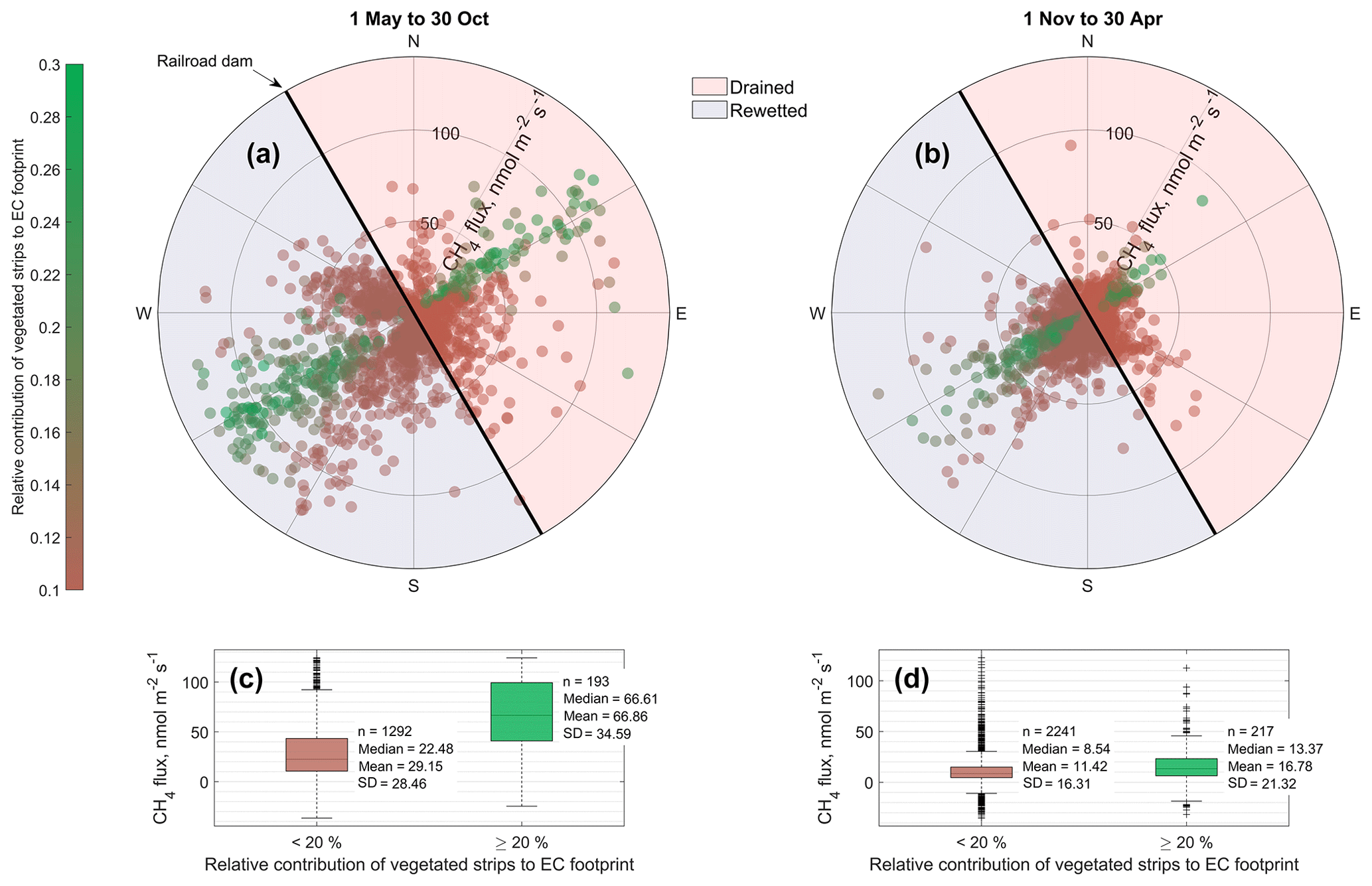
Figure 10 Dependence of methane fluxes on wind direction and eddy covariance (EC) source area composition (in particular the contribution of the vegetated strips) in summer (a) and winter (b). Data of both investigated years are shown. The EC tower was placed on a railroad dam dividing the area into an actively (east) and formerly (west) mined section, which had been rewetted prior to measurements. In general, methane emissions from the rewetted section were higher than from the drained section and fluxes when the EC footprint was composed of more than 20 % vegetated areas was significantly (two-sample Kolmogorov–Smirnov test, p<0.01) higher than from vegetation-free areas, both in summer (c) and winter (d).

The CH₄ flux sums of 13.3±1.8 and 18.3±1.5 g m⁻² a⁻¹ from the rewetted sections of Himmelmoor are confirmed by findings from Beyer and Höper (2015), who report CH₄ balances between 16.2±2.2 and 24.2±5.0 g m⁻² a⁻¹ from inundated cutover bogs in northern Germany. Wilson et al. (2016b) report annual CH₄ emission sums of 12.0±2.6 g m⁻² a⁻¹ from an Irish Atlantic blanket bog that had been rewetted 14 years prior to the investigation. Results from a boreal peat extraction site 20 years after mining had been ceased are given by Tuittila et al. (2000). Although only the growing season has been covered by these authors, the cumulative seasonal $F_{{\mathrm{CH}}_{\mathrm{4}}}$ of 1.27 g m⁻² a⁻¹ suggests that CH₄ release from boreal peatlands is much lower compared to temperate sites. This circumstance has also been noted by Tiemeyer et al. (2016), who furthermore conclude that IPCC estimates for CH₄ release from rewetted bogs, as they are primarily based on data from boreal peatlands, are not representative for temperate regions. In the above-mentioned meta-study of Wilson et al. (2016a), temperate and boreal rewetted peat extraction sites are reported with average emissions of 12.3 g m⁻² a⁻¹. Annual CH₄ release from the drained sections of Himmelmoor (7.2±1.8 and 12.1±1.3 g m⁻² a⁻¹) are lower than from the rewetted parts but high compared to IPCC emission factors. Wilson et al. (2016a) give an average release of 3.3 g m⁻² a⁻¹ for drained peat mining sites, including a 5 % surface cover of ditches to which the authors assign high CH₄ fluxes, as given in Hiraishi et al. (2014) with 10 to 98 g m⁻² a⁻¹. The vegetated strips in Himmelmoor cover around 10 % of the surface (see Fig. 9) and are especially strong sources of CH₄, which we attribute to the high density of vascular, aerenchymatic plants in combination with a supply of nutrient-rich, minerogenic water, which is supplied to these areas from the underlying aquifer. Figure 10 illustrates the dependence of $F_{{\mathrm{CH}}_{\mathrm{4}}}$ on the relative contribution of the vegetated strips to the EC footprint. Mean summer fluxes were significantly (Two-sample Kolmogorov–Smirnov test, p<0.01) higher from the vegetated (67 nmol m⁻² s⁻¹) than from the bare (29 nmol m⁻² s⁻¹) areas. These results are in line with estimates from Vybornova (2017), who determined a mean annual $F_{{\mathrm{CH}}_{\mathrm{4}}}$ of 50 nmol m⁻² s⁻¹ for the same vegetated strips in Himmelmoor with manual chambers. Vybornova et al. (2019) report mean annual $F_{{\mathrm{CH}}_{\mathrm{4}}}$ from the bare peat areas of 10 nmol m⁻² s⁻¹. Further evidence for the decisive role that the type of vegetation established after rewetting has on the magnitude of CH₄ release is provided by Järveoja et al. (2016). The authors report annual CH₄ budgets of 0.25 and 0.16 g m⁻² a⁻¹ at subsections of their site with relatively high and low water table, respectively. The site Järveoja et al. (2016) investigated is the former peat extraction area of Tässi in central Estonia (58^∘ N). In contrast to Himmelmoor, restoration measures at this site included the active establishment (dispersal) of peat mosses on a substantial layer (2.5 m) of remnant Sphagnum spp. peat. By the time measurements commenced 2 years after first restoration efforts were made, Tässi was already dominated by Sphagnum spp. mosses. With a lack of aerenchymatic plants and systematic efforts to re-establish bog vegetation, annual CH₄ release at Tässi is up to 100 times smaller than at Himmelmoor.

3.4 Implications of rewetting measures for the re-establishment of a mire ecosystem in Himmelmoor

In general, the initialization of peat accumulation by Sphagnum mosses is inevitable (Joosten, 1992; Pfadenhauer and Klötzli, 1996; Gaudig, 2002) for the purpose of re-establishing a degraded peatland's natural ecosystem functions. Two (somewhat untypical) features of Himmelmoor need to be considered when evaluating the success of the implemented rewetting measures in terms of mire re-establishment and climate change mitigation: (1) the fact that large vegetation-free areas have been inundated shallowly and (2) that fen-type plants have established in the only vegetated areas that had been taken out of use in the late 1960s. We found peak CH₄ emissions from the vascular-plant-dominated areas (see Fig. 10) and also attribute this fact causally to the presence of fen-type vegetation. Vascular plants provide an effective transport pathway through their gas-conducting tissue and root exudates, which form an easily decomposable substrate for soil microbes (Kerdchoechuen, 2005; Neue et al., 1996; Bhullar et al., 2014). Because a water table above the surface instead of close to but below the surface has been established at the bare peat areas, the creation of floating vegetation mats is the only possibility for Sphagnum colonization (Pfadenhauer and Klötzli, 1996). Nevertheless, fast-growing vascular plants can support peat moss growth by diminishing wave movement and offering adherence area (Sliva, 1997). Besides the need for a preferably calm water surface, another limiting factor for floating mat growth is the water CO₂ concentration (Gaudig, 2002; Paffen and Roelofs, 1991; Smolders et al., 2001; Lamers, 2001; Lütt, 1992), which can be enhanced by vascular plants by providing oxygen to the rhizosphere fostering soil respiration. It thus seems conceivable that the Sphagnum spp. growth-favoring effects could outweigh the negative ramifications for bog development and climate change mitigation potential that the current plant cover implies. In sections of Himmelmoor with a nonindustrial land use history, overgrowth of the grass tussocks (formerly dominating the area) by the bog-type Sphagnum species S. magellanicum and S. papillosum is in progress today (David Holl, personal observation, 2016). The now prevailing plant species on the extraction site could therefore constitute an intermediate state that can potentially be overcome. The active dispersal of Sphagnum mosses as a management strategy would foster mire re-establishment and possibly lead to drastically diminished CH₄ release, as in, e.g., the study from Järveoja et al. (2016) from an Estonian site where peat mosses dominated after rewetting.

4 Conclusions

As a methodological challenge, we addressed the feasibility of a single EC tower for the estimation of gas flux time series from two surface classes within the EC footprint. Due to the specific setup with (1) the tower position on the border between the surface classes and (2) an adequate measurement height of the EC system, we could attribute fluxes to individual surface classes. This subdivision of EC time series was possible owing to the scale (hundreds of meters) on which surface patterning exists in Himmelmoor. Additionally, the contrast in gas flux dynamics between the different surface classes allowed for a better discriminability between EC fluxes associated to the individual surface types. In situations where flux contrasts are less pronounced and surface classes are more interlaced this method might not be applicable. To be able to estimate gas flux time series of subsections within the EC footprint, rigorous filtering of the original time series is inevitable. Consequently, a considerable amount of measurement data are omitted, leading to a relatively high amount of time series gaps. To fill these gaps, we tested multilinear models and artificial neural networks (ANNs) and found that ANNs consistently performed better. We attribute this fact partly to our data-driven model input selection gravely reducing the number of model parameters. Secondly, we programmatically reduced the number of ANN hidden layer neurons, and thereby furthermore lowered the number of model parameters. Apart from the reduction of the model input space dimensionality, our input selection method also outlined physically sound explanatory frameworks for flux–driver connections. Although it cannot ultimately be appraised if the relevant flux drivers have been captured by our routine, the selection results point to the method's ability to discriminate between weaker and stronger flux–driver relations, which do not necessarily have to be linear. We therefore conclude that when applying empirical models to gap-fill trace gas flux time series, a method for the selection of input variables that takes into account the sensitivity of gas fluxes to model input variability can improve model predictions considerably. When ANNs are used in particular, efforts should be made to set them up in the least convoluted way that a sufficient approximation of the target data allows for.

With the estimates of surface-class-specific GHG fluxes from two consecutive years, we could address the impact rewetting had on the GHG balance of the peat mining site. A total of 6 years after the first polders in Himmelmoor had been rewetted, the area was still a clear GHG source. The two investigated land use types (drainage and rewetting) show distinct CO₂ and CH₄ flux features. CO₂ emissions decreased progressively after rewetting with a reduction of 101 g m⁻² a⁻¹ in Year 1 and 407 g m⁻² a⁻¹ in Year 2. The release of CH₄–CO₂ eq. increased after rewetting and was constant in both investigated years (209 g m⁻² a⁻¹). The climate impact of elevated CH₄ emissions after rewetting therefore dominated over the effect of decreasing CO₂ release in Year 1, whereas CO₂ emission reduction was nearly twice as high as the CH₄–CO₂ eq. increase in Year 2. It is conceivable that Himmelmoor can be transformed into a carbon-accumulating peatland. However, this process will probably take decades to centuries and will take place only when sustained management of the area is employed.

Appendix A: Model input variables

Table A1 Model inputs used for methane and carbon dioxide flux gap-filling sorted by type. (x: available; –: not available; n/a: not applicable).

Appendix B: Comparative validation of multilayer perceptron and multilinear regression models

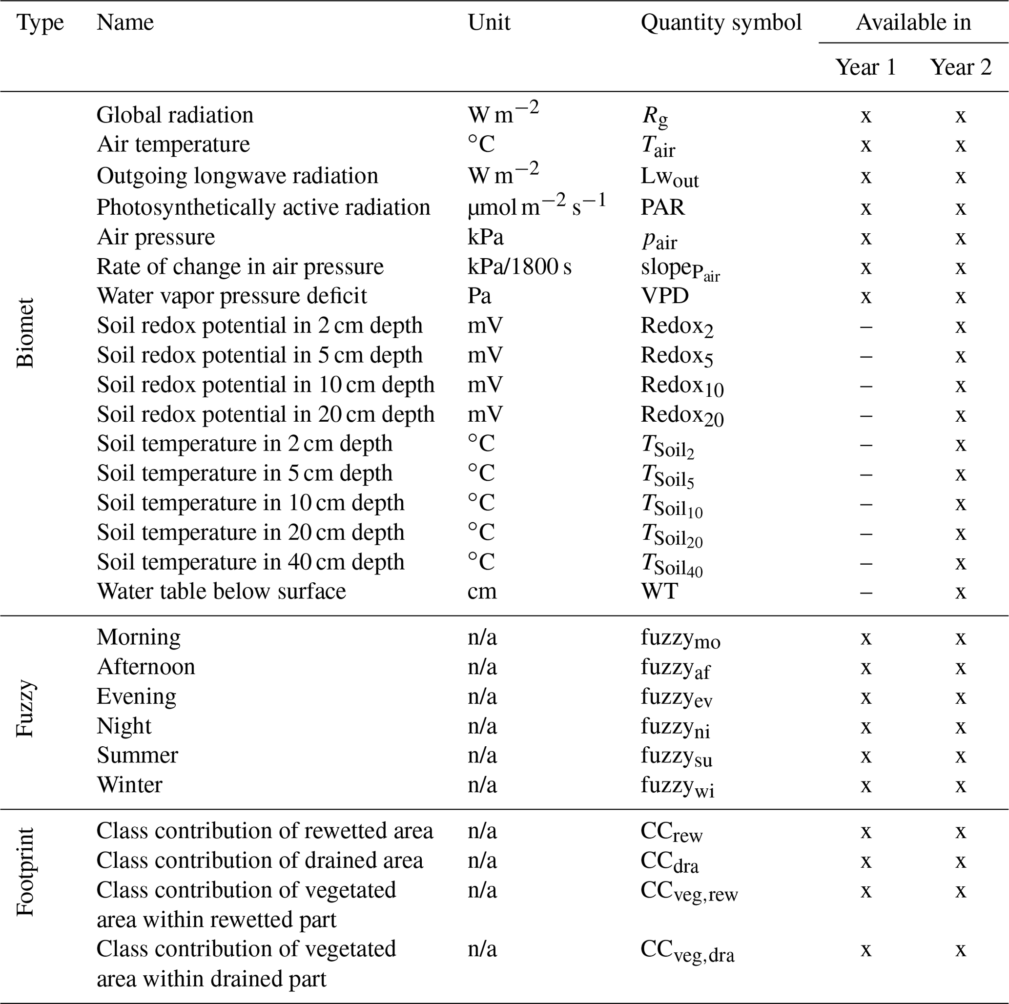
Figure B1 Comparative validation of surface-class-specific multilinear regression and artificial neural network (in particular multilayer perceptron) methane (CH₄) flux models for both investigated years. Multilayer perceptrons appear to be superior with respect to the coefficient of determination (R²), the Akaike information criterion (AIC) and the root-mean-squared error (RMSE) in all cases. Moreover, multilinear regression models tend to be S-shaped and therefore overestimate high and low measured fluxes.

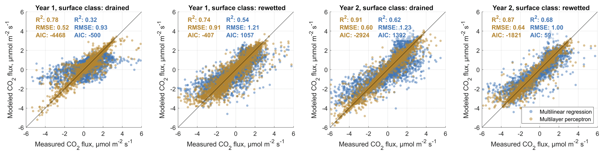
Figure B2 Comparative validation of surface-class-specific multilinear regression and artificial neural network (in particular multilayer perceptron) carbon dioxide (CO₂) flux models for both investigated years. Multilayer perceptrons appear to be superior with respect to the coefficient of determination (R²), the Akaike information criterion (AIC) and the root-mean-squared error (RMSE) in all cases.

Appendix C: Comparison of NEE model parameters with literature values

Vanselow-Algan et al. (2015)Beyer and Höper (2015)Patankar et al. (2013)Körner (1982)Murchie and Horton (1997)Kaipiainen (2009)Patankar et al. (2013); Gu et al. (2008)Lienau (2014)Nygren and Kellomäki (1983)Hoogesteger and Karlsson (1992)Chen et al. (2010)Ögren (1993)Vernay et al. (2016)

Table C1 Total ecosystem respiration (TER_veg, µmol m⁻² s⁻¹), maximum photosynthesis (P_max, µmol m⁻² s⁻¹) and initial quantum yield (α, dimensionless) from the vegetated strips of this study compared to literature values from similar plant species. As the literature record of combined plant and soil respiration measurements of the species that occur at the site of this study is limited, autotrophic respiration (R_a, µmol m⁻² s⁻¹) estimates of plants from the same genera are also given. Note that R_a values were determined on a leaf scale and therefore refer to leaf area. Since shrubs and trees can have a leaf area index larger than 1, fluxes referring to ground surface area could be higher. Model parameter values from this study are given as averages and standard deviation. The latter statistic expresses the value range throughout two annual courses as shown in Fig. 7 rather than parameter uncertainty.

Vanselow-Algan et al. (2015)Vybornova et al. (2019)Waddington et al. (2002)Shurpali et al. (2008)

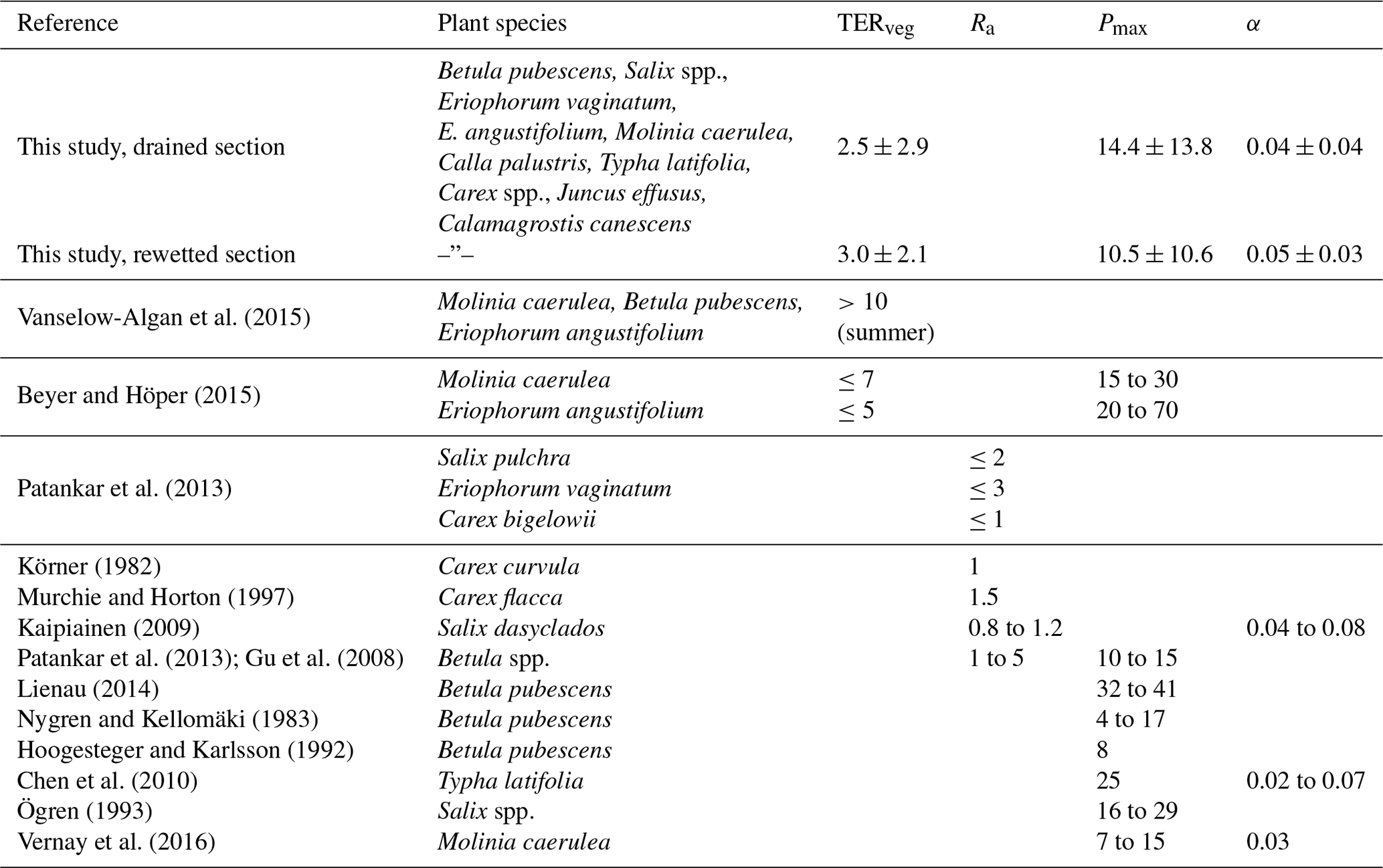
Table C2 Comparison of total ecosystem respiration fluxes from bare peat areas without vegetation (TER_bare) between our study (see Fig. 7a for full time series) and literature values (closed chamber methods) from the same and similar peat extraction sites.