Ecosystem physio-phenology revealed using circular statistics

Quantifying how vegetation phenology responds to climate variability is a key prerequisite to predicting how ecosystem dynamics will shift with climate change. So far, many studies have focused on responses of classical phenological events (e.g., budburst or flowering) to climatic variability for individual species. Comparatively little is known on the dynamics of physio-phenological events such as the timing of maximum gross primary production (DOY_GPPmax), i.e., quantities that are relevant for understanding terrestrial carbon cycle responses to climate variability and change. In this study, we aim to understand how DOY_GPPmax depends on climate drivers across 52 eddy covariance (EC) sites in the FLUXNET network for different regions of the world. Most phenological studies rely on linear methods that cannot be generalized across both hemispheres and therefore do not allow for deriving general rules that can be applied for future predictions. One solution could be a new class of circular–linear (here called circular) regression approaches. Circular regression allows circular variables (in our case phenological events) to be related to linear predictor variables as climate conditions. As a proof of concept, we compare the performance of linear and circular regression to recover original coefficients of a predefined circular model for artificial data. We then quantify the sensitivity of DOY_GPPmax across FLUXNET sites to air temperature, shortwave incoming radiation, precipitation, and vapor pressure deficit. Finally, we evaluate the predictive power of the circular regression model for different vegetation types. Our results show that the joint effects of radiation, temperature, and vapor pressure deficit are the most relevant controlling factor of DOY_GPPmax across sites. Woody savannas are an exception, where the most important factor is precipitation. Although the sensitivity of the DOY_GPPmax to climate drivers is site-specific, it is possible to generalize the circular regression models across specific vegetation types. From a methodological point of view, our results reveal that circular regression is a robust alternative to conventional phenological analytic frameworks. The analysis of phenological events at the global scale can benefit from the use of circular statistics. Such an approach yields substantially more robust results for analyzing phenological dynamics in regions characterized by two growing seasons per year or when the phenological event under scrutiny occurs between 2 years (i.e., DOY_GPPmax in the Southern Hemisphere).

1 Introduction

Phenology is the study of the timing of biological events that can be observed at either the organismic level or the ecosystem scale (Lieth, 1974). For the latter, phenology is the study of some integral behavior across phenological states of the integrated canopy reflectance captured by remote sensing (Richardson et al., 2009; Zhang et al., 2003) or vegetation-driven ecosystem–atmosphere CO₂ exchange fluxes (Richardson et al., 2010). Ecosystem-scale physio-phenological processes of this kind are relevant quantities in global biogeochemical cycles and integrate both the seasonal dynamics of biophysical states (e.g., reflected in the canopy development) and the observed photosynthesis at the stand level (i.e., gross primary production). Here we are particularly interested in the timing when ecosystems reach their maximum CO₂ uptake within a growing season. Ecosystem physio-phenology is influenced by climate conditions but simultaneously contributes to the regulation of different micro- and macrometeorological patterns. Physio-phenological cycles determine the temporal dynamics of land–atmosphere water and energy exchange fluxes. Likewise, the terrestrial carbon cycle is affected by phenological controls on CO₂ uptake and release (Peñuelas et al., 2009).

The eddy covariance (EC) technique allows us to continuously measure the exchange of energy and matter between ecosystems and the atmosphere (Aubinet et al., 2012). The FLUXNET network collects EC data for most ecosystems of the world along with other meteorological variables, i.e., radiation, temperature, precipitation, atmospheric humidity, and often soil moisture (Baldocchi et al., 2001; Baldocchi, 2020). Particularly relevant to phenological studies is the seasonal trajectory of gross primary production (GPP), which allows us to derive phenological transition dates such as start and end of the growing season (e.g., Luo et al., 2018) as well as the timing of the maximum gross primary production, hereafter as referred to as DOY_GPPmax (Zhou et al., 2016; Peichl et al., 2018; Wang and Wu, 2019).

In this study we focus on understanding how climate variability affects the time when ecosystems reach their maximum potential for CO₂ absorption. In order to reach this “optimum state”, several preconditions must be met during the preceding part of the growing season. So far several studies have focused on studying the variability of maximum GPP during the growing season (GPPmax). For instance, Zhou et al. (2017) studied how the variability of annual GPP is influenced by GPPmax and the start and the end of the growing season. The authors found that GPPmax is a better explanatory parameter for the interannual variability of annual GPP than the start and end days of the growing season. Bauerle et al. (2012) studied how photoperiod and temperature influence plants' photosynthetic capacity for 23 tree species in temperate deciduous hardwoods, reporting that the photoperiod explains the variability of photosynthetic capacity better than temperature. So far, to the best of our knowledge, only one study has focused on understanding the temporal variability of GPPmax; Wang and Wu (2019) used a combination of satellite remote-sensing and eddy covariance data to explore how DOY_GPPmax is controlled by climatic conditions. The authors reported that higher temperatures advance DOY_GPPmax, while the influence of precipitation and radiation were biome-dependent. This study had a geographical focus on China; a global approach considering several ecosystems across the whole latitudinal gradient is still lacking.

The challenge of understanding phenology is generally to characterize a discrete event that repeats periodically. Classically, phenological analyses have been performed using linear regression models (Morente-López et al., 2018; Zhou et al., 2016). Most of these studies analyze ecosystems characterized by one growing season (e.g., temperate or boreal forests) and when the summer is centered around the middle of the calendar year. The existing methods are, however, not sufficiently generic to describe (i) ecosystems in the Southern Hemisphere and (ii) ecosystems with multiple growing seasons per year as is often observed in, for example, semiarid regions.

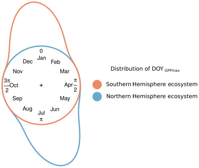
Figure 1 Conceptual distribution of GPPmax timing (DOY_GPPmax) for two hypothetical ecosystems: one in the Northern (blue) and one in the Southern Hemisphere (red). The distance between the color line and the circle represents the frequency of the DOY_GPPmax observations. The distance between the end and the beginning of the distribution represents the DOY_GPPmax interannual variability.

Figure 1 illustrates the problem of northern vs. southern hemispheric summers from a conceptual point of view, assuming that some discrete event recurs annually, but the timing varies according to some external drivers. We would then need to find a predictive model explaining the interannual variability of phenology, i.e., the probability of this recurrent event in the course of the annual cycle. Figure 1 shows that linear regression models would be inappropriate to predict the day of the year (DOY) of some phenological event in the Southern Hemisphere as the actual target values to predict may alternate between $\mathit{⪆}\frac{\mathrm{3}\mathit{\pi }}{\mathrm{2}}$ and $\mathit{⪅}\frac{\mathit{\pi }}{\mathrm{2}}$.

In recent years, circular statistics have gained some attention as they offer a solution to problems of this kind (Morellato et al., 2010; Beyene et al., 2018). Unlike classical statistics, the predicted variables are expressed in terms of angular directions (degrees or radians) across a circumference (Fisher, 1995), allowing us to perform statistical analysis where the data space is not Euclidean. In this framework, point events can be described as a von Mises distribution (Von Mises, 1918), the equivalent to the normal distribution in circular statistics. The von Mises distribution is described by two parameters: the mean angular direction (μ) and the concentration parameter (κ). Circular–linear regressions (in the following simply named circular regression) allow us to predict circular responses (e.g., the timing of phenological events) from other linear variables (Morellato et al., 2010). Given that any phenological event can be interpreted as an angular direction and should be modeled as such, we assume that these circular regressions are well suited in this context. Despite this evident suitability, circular statistics have not yet been extensively applied in the study of phenology and will therefore be presented here as an alternative to conventional linear techniques.

In this paper, we aim to identify the factors controlling the timing of the maximal seasonal GPP (DOY_GPPmax). The questions we want to answer are as follows: first, can circular statistics describe and predict DOY_GPPmax per vegetation type? This aspect requires testing the methodological advantages and caveats of circular statistics across hemispheres in comparison with linear methods. Second, can DOY_GPPmax be explained using cumulative climate conditions? This question needs to consider different possibilities for generating temporally integrating features. And third, how is DOY_GPPmax affected by the climatic conditions during the growing season? The last question requires a global cross-site analysis. Based on the findings of these three questions, we then discuss the potential of circular regressions beyond this specific application case in related phenological problems and outline future applications.

2 Methods

2.1 Data

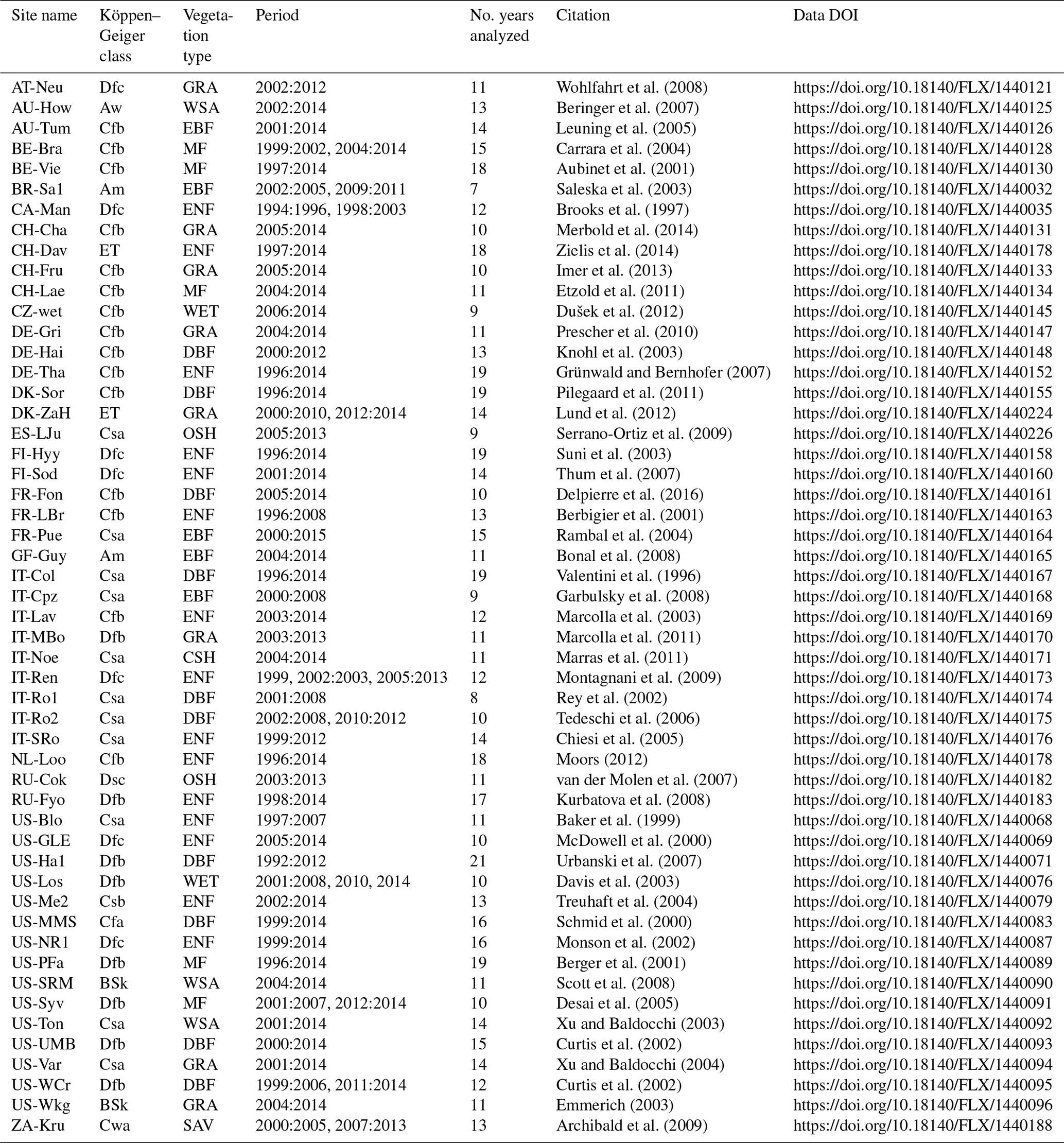
We use 52 EC sites (with at least 7 years of data) located throughout the latitudinal gradient of the globe from the FLUXNET2015 database (Table A1; http://fluxnet.fluxdata.org/, last access: 11 July 2019 Pastorello et al., 2020). Each FLUXNET site is identified with an abbreviation of the country and the name of the place, e.g., the EC tower AU-How, means that it is located in Howard Springs, Australia. From the dataset we use the GPP data that were derived using the nighttime partitioning method and considering the threshold of the variable u^∗ to discriminate values of insufficient turbulence (Reichstein et al., 2005). In order to identify maximum daily GPP, we compute the quantile 0.9 for each day based on the half-hourly flux observations. As potential explanatory variables for DOY_GPPmax we use the daily air temperature (Tair), shortwave incoming radiation (SWin), precipitation (Precip), and vapor pressure deficit (VPD).

Given that the past climate conditions affect the CO₂ exchange between the atmosphere and the ecosystems (ecological memory;  Liu et al., 2019; Ryan et al., 2015), we assume that an aggregated form of these climatic variables needs to be considered in the prediction of the phenological responses. We aggregate the original time series of the Tair, SWin, Precip, and VPD for each DOY_GPPmax using a half-life decay function (Eq. 1),

$$\begin{array}{}\text{(1)}& 〈{\mathbf{x}}_t〉={\displaystyle \frac{{\sum }_{i=\mathrm{0}}^{\mathit{\tau }}{x}_{t-i}{w}_i}{{\sum }_{i=\mathrm{0}}^{\mathit{\tau }}{w}_i}},\end{array}$$

for estimating an exponentially weighted mean of the observation vector ${\mathbf{x}}_t=(x_t,x_{t-\mathrm{1}},\mathrm{\dots },x_{t-\mathit{\tau }}{)}^T$ at time step t. The symbol 〈…〉 denotes the weighted average; i indicates the number of days before t, going back to τ=365 days. The weight decay is represented by

$$\begin{array}{}\text{(2)}& w_i=w_{\mathrm{0}}\exp \left(-i{\displaystyle \frac{\ln \left(\mathrm{2}\right)}{t_{\mathrm{1}/\mathrm{2}}}}\right).\end{array}$$

The decay function gives the instantaneous value a weight of 1 (w₀=1), and all preceding values receive an exponentially reduced weight as determined by the half-time parameter t_1∕2. Finally, we make these variables comparable via centering standardization to unit variance. We perform a sensitivity analysis, evaluating the effect of the half-time parameter, and identify the optimum as the value when the variance explained by the circular regression model is at a maximum. The results are presented in Supplement 1.

Due to the high colinearity between the exponential weighted variables of Tair, SWin, and VPD, we perform a principal component analysis (PCA) on the matrix of variables and FLUXNET sites and retain the leading principal component of these variables as well as precipitation as input for the circular statistics model (Hastie et al., 2009). The results of the PCA are presented in Supplement 2.

2.2 Circular statistics

Since units of the circular response variable must be in radians or degrees, we transform the days of the year to radians using Eq. (3). For leap years we remove the last day.

$$\begin{array}{}\text{(3)}& \mathrm{rad}=\mathrm{DOY}{\displaystyle \frac{\mathrm{360}}{\mathrm{365}}}{\displaystyle \frac{\mathit{\pi }}{\mathrm{180}}},\end{array}$$

where DOY means day of the year.

A basic circular regression model was proposed by Fisher and Lee (1992) as follows:

$$\begin{array}{}\text{(4)}& y=\mathit{\mu }+\mathrm{2}\mathrm{atan}\left({\mathit{\beta }}_i{x}_i\right),\end{array}$$

where y is the target variable (i.e., DOY_GPPmax) in radians, μ is the mean angular direction of the target variable, x_i represents the values for the variable i, and β_i is the regression coefficient. The parameters μ and β are fitted via the maximum likelihood method using the reweighted least squares algorithm as proposed by Green (1984).

Relevant interpretations of fitted circular regression models are (1) the sign of the β coefficients, (2) the statistical significance of the coefficients, and (3) the accuracy of the prediction. Regarding the first point, a negative sign of the coefficient would mean that an increasing value of the predictor would lead to an earlier DOY_GPPmax compared to the mean angular direction. The inverse would happen when the coefficient is positive. Figure 2 conceptually illustrates how the coefficients affect the predictions. Regarding the second aspect, we can state that if a coefficient is not significant, then its contribution would not be relevant to explaining the phenological observation. In our case we define the coefficient to be significant if the median of the distribution of p values is less than 0.05. Finally, we can estimate the accuracy of the prediction using the Jammalamadaka–Sarma (JS) correlation coefficient (Jammalamadaka and Sarma, 1988). As in any other regression framework, this approach helps us to quantify the effect of each climate variable on the interannual variability of DOY_GPPmax.

To estimate the relative sensitivity of DOY_GPPmax to the leading principal component representing Tair, SWin, and VPD as well as to Precip, we use the implementation of Eq. (4) in the R package “circular” (Agostinelli and Lund, 2017). To increase the robustness of the method we implemented a block bootstrapping per growing season, generating a model parameter average based on 1000 iterations. In each analysis, we estimate the accuracy of the model using the JS correlation coefficient.

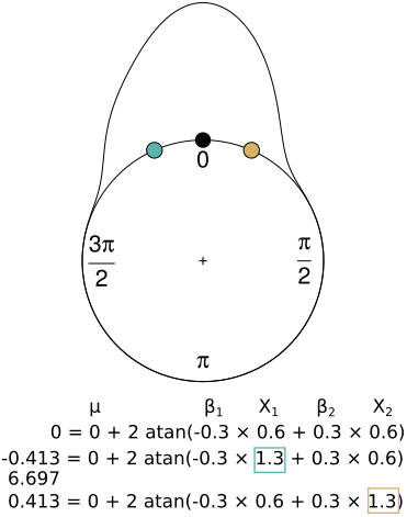
Figure 2 Interpretation of the coefficients in the circular regression considering a reference point (black) generated with a circular–linear model with mean angular direction (μ=0), two coefficients (β₁, β₂) and two variables (x₁, x₂), where one of the coefficients is negative (β₁), and the other one is positive (β₂). When the coefficient is negative and the value of the parameter increases (blue), the result is an earlier observation compared with the reference point (the equivalent of −0.413 rad is 6.697 rad, as is shown below the equation). On the other hand, when the coefficient is positive and the variable increases (yellow), the observation is later.

2.3 Circular vs. linear regression

To assess the performance of linear versus circular regressions we perform an experiment with simulated data in which we evaluate the accuracy and precision of both approaches to recover original regression coefficients in a circular setting (Eq. 4). We add noise generated with a random von Mises distribution with the parameters n=100 and κ=30 to the model to ensure that the result follows a normal distribution. We predefined a range of values for two regression coefficients (${\mathit{\beta }}_{\mathrm{1}}=\langle \mathrm{0.01},\mathrm{\dots },\mathrm{3}\rangle$, ${\mathit{\beta }}_{\mathrm{2}}=\langle \mathrm{0.01},\mathrm{\dots },\mathrm{3}\rangle$). We simulate the variables x₁ and x₂ as normal distributions with n=100; a mean of 10 and 15, respectively; and standard deviations (SDs) of 1 and 2. We evaluate all possible combinations for the regression coefficients 100 times, simulating different x₁ and x₂. In each iteration we generate y using the setup previously described, and we recover the original regression coefficients using y as a response variable and x₁ and x₂ as predictors. Finally, we analyze two scenarios: (1) when the target timing occurs at the beginning of the year (μ=0) and (2) when the target timing happens midyear (μ=π). The parameters for the entire setup generate realistic data, where the standard deviation of y is not higher than 0.3 rad. An SD of 0.5 rad would be equivalent to having phenological observations across half a year, which would not be realistic.

To quantify the accuracy of each model per coefficient we estimate the mean absolute error per model and coefficient (Eq. 5). To compare the accuracy between models by coefficient we test the mean absolute errors between models (Eq. 6). To generate a single measure that allows us to compare both coefficients and models we estimate the mean difference accuracy (Eq. 7). The results can be understood as follows: if the difference is higher than 0, the circular model has a higher mean accuracy compared to the linear model and vice versa. To quantify which model has higher precision we estimate the difference between the SD of the mean absolute errors per model for each coefficient (Eq. 8). Finally, we estimate the mean differences of precision between the regression coefficients (Eq. 9), where again if the value is higher than 0, the circular model has a higher mean accuracy than the linear model; the inverse is true if the value is lower than 0.

We estimate regression coefficients for the bootstrap sample $i\in \mathit{\{}\mathrm{1},\mathrm{\dots },m\mathit{\}}$ (m=100) for the regression coefficient β_j, $j\in \mathit{\{}\mathrm{1},\mathrm{2}\mathit{\}}$, and the model $M\in \mathit{\{}l,c\mathit{\}}$ (denoted as ${\widehat{\mathit{\beta }}}_{j,i}^M$). The model accuracy can then be estimated as the mean absolute error of the estimated regression parameter ${\widehat{\mathit{\beta }}}_j^M$, $j\in \mathit{\{}\mathrm{1},\mathrm{2}\mathit{\}}$ for the linear model M=l and the circular model M=c:

$$\begin{array}{}\text{(5)}& {\displaystyle }{a}_{M,j}{\displaystyle }={\displaystyle \frac{\mathrm{1}}{m}}\sum _{i=\mathrm{1}}^m|{\widehat{\mathit{\beta }}}_{j,i}^M-{\mathit{\beta }}_j|.\end{array}$$

The difference in accuracy for the coefficient j between the circular and the linear model is shown in

$$\begin{array}{}\text{(6)}& {\displaystyle }{\mathit{\delta }}_{a,j}{\displaystyle }=a_{l,j}-a_{c,j}.\end{array}$$

Finally, the mean difference in accuracy between the linear and the circular model is given by

$$\begin{array}{}\text{(7)}& {\displaystyle }{\mathit{\delta }}_a{\displaystyle }={\displaystyle \frac{{\mathit{\delta }}_{a,\mathrm{1}}+{\mathit{\delta }}_{a,\mathrm{2}}}{\mathrm{2}}}.\end{array}$$

The difference in precision for the coefficient j between the linear (l) and the circular model (c) is shown in

$$\begin{array}{}\text{(8)}& {\displaystyle }{\mathit{\delta }}_{p,j}{\displaystyle }={\mathrm{s}}_{l,j}-{\mathrm{s}}_{c,j}.\end{array}$$

The mean difference in precision between the linear and the circular model is given by

$$\begin{array}{}\text{(9)}& {\displaystyle }{\mathit{\delta }}_p{\displaystyle }={\displaystyle \frac{{\mathit{\delta }}_{p,\mathrm{1}}+{\mathit{\delta }}_{p,\mathrm{2}}}{\mathrm{2}}},\end{array}$$

where s_M,j is the sample SD of the vector $({\widehat{\mathit{\beta }}}_{j,i}^M{)}_i$, $M\in \mathit{\{}l,c\mathit{\}}$.

2.4 Analysis setup

The target variable DOY_GPPmax is the day of the year when GPP reaches its maximum during the growing season. Given that different ecosystems present more than one growing season per year (e.g., semiarid ecosystems), it is necessary to identify the number of growing seasons per year. To identify the number of growing seasons we apply a fast Fourier transformation (FFT; Cooley and Tukey, 1965) to the mean seasonal cycle of the GPP time series. The number of growing seasons is equal to the maximum absolute value of the first four FFT coefficients (excluding the first one). For each FLUXNET site, we reconstruct the GPP time series, taking the real numbers of the inverse FFT. We use these reconstructed time series to calculate the expected mean timing of DOY_GPPmax and use this value as a template. To recover the real DOY_GPPmax from the original time series, we define a window around the template of length inversely proportional to the number of cycles (180 d∕number of growing seasons). To increase the robustness of the analysis we identify the days with the 10 highest GPP values. These days are used in the block bootstrapping mentioned above. Finally, since most of the sites are located in the Northern Hemisphere we expect that, in most cases, DOY_GPPmax will be reached by the middle of the calendar year.

To quantify the contribution of each climate variable, we count the number of sites per vegetation type where the regression coefficient is statistically significant. We perform a leave-one-out cross-validation per vegetation type to evaluate the predictive power of the circular regression using climate conditions. We only consider vegetation types with more than five sites. In this case the standardization of the climate variables is not applied. Finally, we use the mean of the optimum half-time parameter per vegetation type to weigh the climate conditions.

3 Results

Here, we first report results from simulated data to describe the performance of the circular regression approach compared to a linear model. Second, we compare the performance of circular and linear regression using empirical data. Third, we analyze the sensitivity of DOY_GPPmax across vegetation types and climate classes. Finally, we show the results of the predictive power of circular regression per vegetation type.

3.1 Circular vs. linear regression

Figure 3a and c show that for μ=0 (DOY_GPPmax at the beginning of the year), circular regression has a higher accuracy and precision compared to the linear regression for the entire space of regression coefficient values, with a maximum difference of the order of 0.1 in terms of accuracy and of the order of 1 for precision. For μ=π (DOY_GPPmax midyear) the linear model has a higher accuracy in most of the evaluated space, with a maximum difference of the order of 0.001 compared with the circular regression, while circular regression has a higher precision for most of the regression coefficients of the order of 0.001. These results show that circular regression has a higher precision in recovering the original regression coefficients than linear regression no matter the moment of the year. On the other hand, circular regression has a higher accuracy than the linear model at the beginning of the year. While linear is better midyear, the differences are of the order of 0.001.

Figure 3 Accuracy and precision of linear and circular regression models by recovering the original regression coefficients of a circular regression. (a, c) μ=0 (maximum at the beginning of the year). (b, d) μ=pi (maximum midyear). Panels (a) and (b) correspond to the differences in accuracy between the models. Panels (c) and (d) correspond to the differences in the precision between the models. Blue means better performance of the circular model compared with the linear model, and red means higher performance of the linear model.

To illustrate the method in practice, we compare the circular and linear models using data from two sites: US-Ha1 (Northern Hemisphere, deciduous broadleaf forest) and AU-How (Southern Hemisphere, woody savanna). We relate the climate variables with DOY_GPPmax (see Methods) and reconstruct the DOY_GPPmax using the linear and circular regression models. We compare observed and predicted DOY_GPPmax using JS correlation for the circular model and the Pearson product moment for the linear model. For US-Ha1 both methods show similar performance in predicting DOY_GPPmax (Fig. 4), while for AU-How, the circular model retrieves the original data better than the linear model, explaining 30 % more of the variance. In the event that the DOY_GPPmax is reached at the beginning of the year, linear methods produce a strong bias that predicts the timing across the entire year (Fig. 4b).

Figure 4 Correlation coefficient between the observed and predicted DOY_GPPmax using climatic variables. Two sites are presented: (a) US-Ha1 and (b) AU-How. The observed DOY_GPPmax (green) is compared with the data retrieved using circular (orange) and linear (purple) regressions. Two correlation coefficients are used: Jammalamadaka–Sarma (JS) and the Pearson product moment (Pearson). In the circular plot the months and the day of the year (DOY) are also plotted every 75 d. The green arrow indicates the mean angular direction of the original data distribution.

3.2 Sensitivity of DOY_GPPmax to climate variables

From the 52 sites analyzed in this study, only one site (ES-LJu) shows bimodal growing seasons (see Supplement 1.2). As expected, in most cases DOY_GPPmax occurs in the middle of the calendar year (Fig. S6 in the Supplement), reflecting the uneven site distribution in FLUXNET (Schimel et al., 2015). However, some ecosystems in the Northern Hemisphere do reach DOY_GPPmax at the beginning of the year; these are Mediterranean sites such as US-Var and ES-LJu. In general terms, most of the sites have an SD between 10 d and 40 d. The maximal SD is 46.9 d for the AU-Tum site. A detailed table with the mean angular direction and SD of DOY_GPPmax of each site is presented in Sect. S1.2.

For half of the sites, the JS correlation coefficients are between 0.70 and 0.97 (Supplement 1, Fig. S5), showing that the interannual variability of DOY_GPPmax is mainly explained by the cumulative effect of the climate variables. Nineteen sites have a JS coefficient of less than 0.7 (DK-Sor, FI-Hyy, US-MMS, DK-ZaH, FR-Pue, US-UMB, AU-Tum, US-Ton, FR-LBr, US-Me2, IT-Lav, AT-Neu, DE-Gri, IT-MBo, IT-Ro2, US-Wkg, BR-Sa1, FR-Fon, CZ-wet). For ES-LJu the JS coefficient is 0.77 for the first growing season and 0.78 for the second one (Table S2 in the Supplement).

We find that air temperature, shortwave incoming radiation, and vapor pressure deficit appear as the dominant drivers worldwide at 43 of the total sites (84 %; Supplement 3). Precipitation is the main driver for five sites (AU-How US-Ton ZA-Kru US-SRM US-Wkg; Supplement 3). Interestingly, precipitation was the most important factor for all the woody savanna sites (Supplement 3). For three sites (DE-Gri, IT-Ro2, BRSa1), any climatic variable is significant. In terms of the sign of the coefficients, all the variables are predominantly negative (Table 1). This means that higher values of radiation, air temperature, VPD, and precipitation lead to an earlier DOY_GPPmax. Individual sensitivities per site are shown in Supplement 3.

Table 1 Number of FLUXNET sites where each regression coefficient is statistically significant to explain the physio-phenology of GPPmax (DOY_GPPmax). The table is divided by the sign of the coefficient. The first column is the coefficient for the dimensionality reduction between air temperature (Tair), shortwave incoming radiation (SWin), and vapor pressure deficit (VPD); the second column is the coefficient for precipitation (Precip).

The PCA between shortwave incoming radiation, air temperature, and vapor pressure deficit has the highest frequency of significant correlation coefficients by number of sites for all the vegetation types with the exception of woody savannas (WSAs), where precipitation is shown to be more important for most sites than the dimensionality reduction between Tair, SWin, and VPD (Fig. 5). For closed shrublands (CSHs) and savannas (SAVs), both drivers have the same number of sites where the coefficients are statistically significant.

Figure 5 Contribution of each climate variable to explain the interannual variation in DOY_GPPmax per vegetation type. CSHs: closed shrublands (n=1); DBF: deciduous broadleaf forest (n=10); EBF: evergreen broadleaf forest (n=5); ENF: evergreen needleleaf forest (n=15); GRA: grassland (n=8); MF: mixed forest (n=5); OSHs: open shrublands (n=1); SAV: savannas (n=1); WET: permanent wetlands (n=2); WSAs: woody savannas (n=3). Each bar shows the cumulative number of sites where each climate variable is statistically significant.

A special case for understanding the sensitivity of DOY_GPPmax to climate variables is the site “Llano de los Juanes” (ES-LJu), an open shrubland ecosystem in Spain. It is the only clearly bimodal ecosystem in our study (Fig. 6). In this case precipitation is not statistically significant, while the combination of Tair, SWin, and VPD is significant for both seasons. Furthermore, in both growing seasons Tair, SWin, and VPD have a negative coefficient.

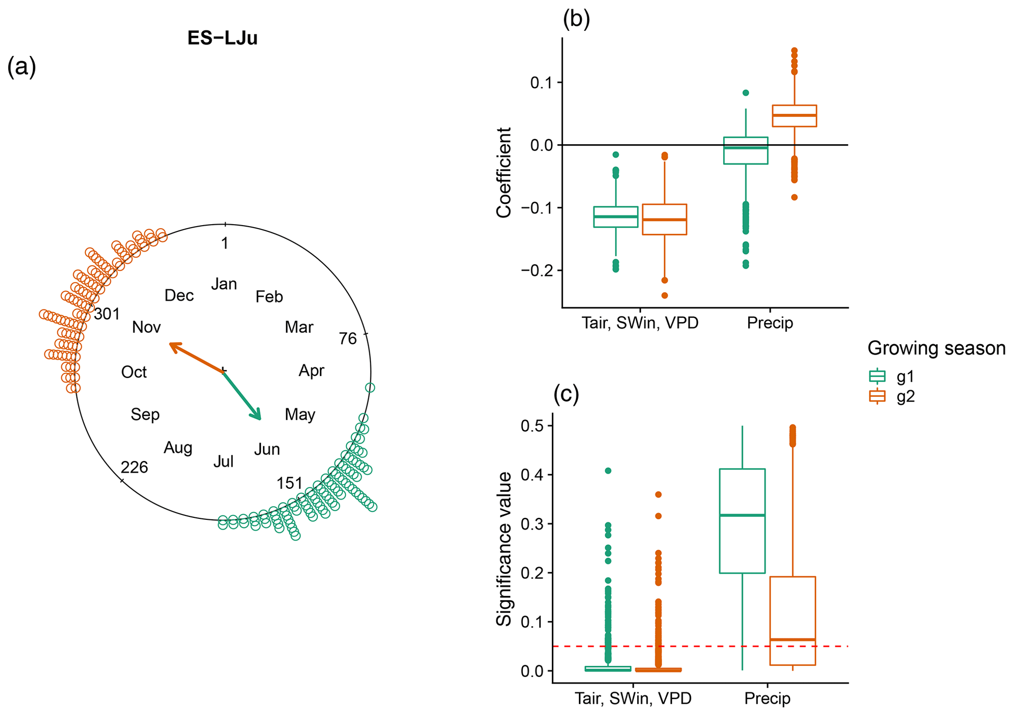
Figure 6 DOY_GPPmax sensitivity to different climate drivers in a Mediterranean ecosystem: Llano de los Juanes (ES-LJu), Spain, with two growing seasons (green and orange). (a) DOY_GPPmax distribution across the year. The arrows indicate the mean angular direction of the growing season. (b) Regression coefficients for each growing season and (c) the significance values for each variable. The red line in panel (c) represents a p value of 0.05.

The leave-one-out cross-validation for several vegetation types shows that the predictive power of the model for grassland (GRA) and evergreen broadleaf forest (EBF) is −0.3 and −0.31, respectively. For deciduous broadleaf forest (DBF) it is 0.46, and for evergreen needleleaf forest (ENF) it is 0.4, while for mixed forest (MF) the predictive power of the model is 0.88 (Fig. 7).

Figure 7 Cross-validation of the circular regression model to predict DOY_GPPmax for different vegetation types using air temperature, shortwave incoming radiation, precipitation and vapor pressure deficit (see Methods). Deciduous broadleaf forest (DBF), evergreen broadleaf forest (EBF), grassland (GRA), mixed forest (MF), and evergreen needleleaf forest (ENF). For each vegetation type the Jammalamadaka–Sarma (JS) correlation coefficient is shown in the title of each plot. The red line represents the perfect fit.

4 Discussion

4.1 Circular vs. linear regression

We explored whether circular regression is a suitable tool for analyzing phenological events. Our results suggest that circular regressions can recover predefined coefficients in a set of simulations with higher accuracy and precision than linear regressions. Hence, we would generally suggest that circular regressions may be advantageous when the aim is analyzing the effect of climatic variables on phenological events. We also found cases where the classical linear regression may be either more robust or equally suitable, e.g., when phenological events are reached close to midyear. In the overall view, however, we consider that circular regressions are to be preferred over linear regression for their conceptual capacity to analyze the physio-phenology of ecosystems regardless of the day of the year when an event of interest occurs. This allows us to analyze phenological studies at the global scale regardless of geographic location or the distribution of the observations during the year.

Different phenological models have been developed, ranging from empirical approaches (Richardson et al., 2013) to process models (Asse et al., 2020) over the last decades. As we demonstrate here, circular statistics open new opportunities to increase the robustness of phenological models, allowing us to analyze ecosystems across hemispheres within the same consistent framework. In fact, the results of the phenological sensitivity of DOY_GPPmax indicate the complexity of ecosystem responses to climate variability. Our approach provides motivation to integrate circular regressions into more complex statistical techniques like regression trees, Gaussian processes, or artificial neural networks, targeting a circular response variable.

4.2 Sensitivity of DOY_GPPmax to climate variables

The geographical location of the FLUXNET2015 sites represents an advantage when capturing the DOY_GPPmax variability at the global scale (Supplement 1, Fig. S6). Most of the analyzed sites (47) are located in the Northern Hemisphere. Two sites (GF-Guy and BR-Sa1) are located in the tropical region, and three sites (ZA-Kru, AU-How, AU-Tum) are in the Southern Hemisphere. However, because of the low number of sites reported in the tropical and southern region with more than 7 years of data, our understanding of the DOY_GPPmax variability in these regions is still limited. Increasing the number of tropical and Southern Hemisphere sites should be considered a high priority in the near future to complement our knowledge about the physio-phenological ecosystem state.

The high values of the JS correlation coefficients for most of the sites demonstrate that the interannual variability of DOY_GPPmax can be explained as the cumulative effect of the climate variables during the growing season. Sites where it was not possible to explain the variations in DOY_GPPmax with enough confidence (JS correlation <0.7) might require the incorporation of biotic variables (e.g., species composition; Peichl et al., 2018) or soil property information that can improve the predictive power of the model.

Our results suggest that there is no pattern between the DOY_GPPmax sensitivity across vegetation types and climate classes (Sect. Fig. S1.7). In other words, the DOY_GPPmax sensitivity is site-specific, probably produced by the unique combination of biotic (e.g., species composition, species phenology, species interaction, and phenotypic plasticity) factors that are not evaluated in our study. Several studies that focused on ecosystem phenology suggest that species composition plays a fundamental role in ecosystem physio-phenology of the CO₂ uptake (Gonsamo et al., 2017; Peichl et al., 2018).

While there is no clear relationship between the DOY_GPPmax sensitivity and the vegetation type, we find a predominant role of the combined effects of shortwave incoming radiation (SWin), air temperature (Tair), and vapor pressure deficit (VPD) at the global scale on the DOY_GPPmax interannual variability, where for most of the sites these variables have a negative regression coefficient. This means that if the SWin, Tair, and VPD increase during the growing season, the DOY_GPPmax will be reached earlier. This effect can be a consequence of DOY_GPPmax being reached when SWin and Tair are at a maximum.

On a global scale, our analysis shows that the combination of air temperature, shortwave incoming radiation, and vapor pressure deficit as well as precipitation has a negative sign. This means that if these variables increase during the growing season, the GPPmax will be reached earlier. Our results are similar to those obtained by Wang and Wu (2019), who were the authors to conclude that an increase in the temperature produces an earlier DOY_GPPmax. This phenomenon is likely explained by the leaf-out advancing during spring. Nevertheless, there is still no consensus on whether the increase in temperature will produce an earlier end of the growing season. Several studies have demonstrated for different vegetation types that when temperature increases, spring onset is earlier, and autumn senescence is later (Stocker et al., 2013; Linkosalo et al., 2009; Migliavacca et al., 2012; Morin et al., 2010; Post and Forchhammer, 2008), increasing the length of the growing season and the amount of CO₂ that is taken up by ecosystems (Richardson et al., 2013).

Ecosystems with two growing seasons per year represent a very interesting case of the effect of climate drivers on DOY_GPPmax across different growing seasons. In Llano de los Juanes, Spain (ES-LJu; Fig. 6), DOY_GPPmax is reached in the first growing season, when the rainy season is finishing, while in the second growing season DOY_GPPmax is reached in the middle of the rainy season (data not shown). The effect of shortwave incoming radiation, temperature, and vapor pressure deficit for both growing seasons is negative, suggesting that if we increase these variables during the period before, the DOY_GPPmax will happen earlier.

Phenology in Mediterranean ecosystems is mainly controlled by water availability (Kramer et al., 2000; Luo et al., 2018; Peñuelas et al., 2009). However, our results suggest that DOY_GPPmax is mainly sensitive to SWin, Tair, and VPD. These results agree with the analysis performed by Gordo and Sanz (2005), who were the authors to evaluate the phenological sensitivity of Mediterranean ecosystems to temperature and precipitation. They concluded that temperature was the most important driver. Although water is a limiting factor in Mediterranean ecosystems, its influence on plant physiology and plant phenology can be completely different. In terms of physiology, the GPPmax value can decrease, but in terms of phenology, DOY_GPPmax can still be the same.

Complex interactions between climate variables and phenological response and the interspecificity of the sensitivity at the site level explain in part the poor predictive power of the model for grasslands, evergreen broadleaf forest, evergreen needleleaf forest, and deciduous broadleaf forests in the cross-validation analysis (Fig. 7). However, the predictive power for mixed forest is high, even when the distribution of the latitudinal gradient is not the same for all the sites. These results reflect the fact that the circular regression model can be extrapolated from different sites to predict the DOY_GPPmax interannual variability. This advantage could be a way to solve the common criticism that phenological models cannot be extrapolated by only generating ad hoc hypotheses (Richardson et al., 2013).

5 Conclusions

In this study we explored the potential of “circular regressions” to explain the physio-phenology of maximal CO₂ uptake rates. We conclude that (1) shortwave incoming radiation, temperature, and vapor pressure deficit are the main drivers of the timing of maximal CO₂ uptake at the global scale (precipitation only plays a secondary role, with the exception of woody savannas, where the most important variable is precipitation), and (2) although the sensitivity of the DOY_GPPmax to the climate drivers is site-specific, it is possible to extrapolate the circular regression model for different sites with the same vegetation type and similar latitudes. Finally, we used simulated and empirical data to demonstrate that circular regression produces more accurate results than linear regression, in particular in cases when data need to be explored across hemispheres.

Appendix A: FLUXNET sites

Wohlfahrt et al. (2008)Beringer et al. (2007)Leuning et al. (2005)Carrara et al. (2004)Aubinet et al. (2001)Saleska et al. (2003)Brooks et al. (1997)Merbold et al. (2014)Zielis et al. (2014)Imer et al. (2013)Etzold et al. (2011)Dušek et al. (2012)Prescher et al. (2010)Knohl et al. (2003)Grünwald and Bernhofer (2007)Pilegaard et al. (2011)Lund et al. (2012)Serrano-Ortiz et al. (2009)Suni et al. (2003)Thum et al. (2007)Delpierre et al. (2016)Berbigier et al. (2001)Rambal et al. (2004)Bonal et al. (2008)Valentini et al. (1996)Garbulsky et al. (2008)Marcolla et al. (2003)Marcolla et al. (2011)Marras et al. (2011)Montagnani et al. (2009)Rey et al. (2002)Tedeschi et al. (2006)Chiesi et al. (2005)Moors (2012)van der Molen et al. (2007)Kurbatova et al. (2008)Baker et al. (1999)McDowell et al. (2000)Urbanski et al. (2007)Davis et al. (2003)Treuhaft et al. (2004)Schmid et al. (2000)Monson et al. (2002)Berger et al. (2001)Scott et al. (2008)Desai et al. (2005)Xu and Baldocchi (2003)Curtis et al. (2002)Xu and Baldocchi (2004)Curtis et al. (2002)Emmerich (2003)Archibald et al. (2009)

Table A1 FLUXNET sites used in our study. We report the name of the sites, the time period used for the analysis, and the climate class of each site following Köppen–Geiger classification: tropical monsoon climate (Am), tropical savanna climate (Aw), cold semiarid climate (BSk), humid subtropical climate (Cfa), oceanic climate (Cfb), hot summer Mediterranean climate (Csa), warm summer Mediterranean climate (Csb), humid subtropical climate (Cwa), humid continental climate (Dfb), subarctic climate (Dfc, Dsc), and tundra climate (ET). We also report the vegetation type of the sites: closed shrubland (CSH), deciduous broadleaf forest (DBF), evergreen broadleaf forest (EBF), evergreen needleleaf forest (ENF), grassland (GRA), mixed forest (MF), open shrubland (OSH), savanna (SAV), permanent wetland (WET), and woody savanna (WSA).