Reconstructing extreme climatic and geochemical conditions during the largest natural mangrove dieback on record

A massive mangrove dieback event occurred in 2015–2016 along ∼1000 km of pristine coastline in the Gulf of Carpentaria, Australia. Here, we use sediment and wood chronologies to gain insights into geochemical and climatic changes related to this dieback. The unique combination of low rainfall and low sea level observed during the dieback event had been unprecedented in the preceding 3 decades. A combination of iron (Fe) chronologies in wood and sediment, wood density and estimates of mangrove water use efficiency all imply lower water availability within the dead mangrove forest. Wood and sediment chronologies suggest a rapid, large mobilization of sedimentary Fe, which is consistent with redox transitions promoted by changes in soil moisture content. Elemental analysis of wood cross sections revealed a 30- to 90-fold increase in Fe concentrations in dead mangroves just prior to their mortality. Mangrove wood uptake of Fe during the dieback is consistent with large apparent losses of Fe from sediments, which potentially caused an outwelling of Fe to the ocean. Although Fe toxicity may also have played a role in the dieback, this possibility requires further study. We suggest that differences in wood and sedimentary Fe between living and dead forest areas reflect sediment redox transitions that are, in turn, associated with regional variability in groundwater flows. Overall, our observations provide multiple lines of evidence that the forest dieback was driven by low water availability coinciding with a strong El Niño–Southern Oscillation (ENSO) event and was associated with climate change.

1 Introduction

Mangroves provide a wide range of ecosystem services, including nursery habitat, carbon sequestration and coastal protection (Barbier et al., 2011; Donato et al., 2011). Climate change is a major threat to mangroves, which adds to existing stressors imposed by deforestation and over-exploitation (Hamilton and Casey, 2016; Richards and Friess, 2016). Sea level rise, altered sediment budgets, reduced water availability and increasing climatic extremes are all negatively affecting mangroves (Gilman et al., 2008; Alongi, 2015; Lovelock et al., 2015; Sippo et al., 2018).

In Australia, an extensive mangrove dieback event in the Gulf of Carpentaria from December 2015 to January 2016 coincided with extreme drought and low regional sea levels. This extreme climatic event drove the largest recorded mangrove mortality event (∼1000 km coastline, ∼7400 ha) attributed to natural causes (Duke et al., 2017; Harris et al., 2017; Sippo et al., 2018) and led to extensive changes in the coastal carbon cycle (Sippo et al., 2019, 2020) and coastal food webs (Harada et al., 2020). Two other large-scale mangrove dieback events occurred at the same time: one in Exmouth (Lovelock et al., 2017) and the other in Kakadu National Park, Australia (Asbridge et al., 2019).

Mangrove mortality has been previously attributed to low water availability associated with extreme drought. Limited rainfall and groundwater availability combined with anomalously low sea levels effectively reduced tidal inundation and soil water content (Duke et al., 2017; Harris et al., 2017). A strong El Niño event had resulted in the lowest recorded rainfall in the 9 months preceding the mangrove dieback since 1971 and had been accompanied by regional sea levels that were 20 cm lower than average (Harris et al., 2017). Atmospheric moisture was also unusually low during 2015 – a feature which may influence the physiological functioning of mangrove trees (Nguyen et al., 2017). Such severe climatic and hydrologic changes may affect both plant physiology and sediment geochemistry.

In contrast to terrestrial forest soils, mangrove sediments are largely anoxic due to their waterlogged nature and high organic matter contents. Mangrove sediments also receive a supply of materials from both terrestrial environments (e.g. Fe, sediments) and oceanic water (e.g. SO₄) which results in distinctly different biogeochemical cycling than terrestrial forests (Burdige, 2011). As a result, mangrove sediments often accumulate substantial (∼1 %–5 %) bioauthigenic pyrite (FeS₂). Pyrite remains stable under waterlogged and reducing conditions (van Breemen, 1988; Johnston et al., 2011). However, lowering of water levels can alter sediment redox conditions and result in rapid oxidation of FeS₂, releasing acid and dissolved Fe (mostly as more soluble Fe²⁺ species) to porewaters (Burton et al., 2006; Johnston et al., 2011; Keene et al., 2014). Subsequent oxidation of Fe²⁺ and precipitation of Fe(III) (oxy)hydroxide minerals can then lead to the accumulation of highly reactive Fe in sediments. Such reactive Fe(III) minerals are, in turn, readily subject to reductive dissolution and (re)-formation of soluble Fe²⁺ species during any subsequent switch to more reducing conditions. Thus, changes in sediment redox conditions (e.g. increased oxidation and subsequent reduction) in mangrove sediments that are rich in FeS₂ can cause a release of relatively mobile and bioavailable Fe²⁺ during the redox transition(s).

Mobilization of Fe due to fluctuating oxidation–reduction cycles could also have important consequences for coastal Fe cycling. For example, Fe is often a limiting nutrient in ocean surface waters and, thus, Fe outwelling from mangroves could have important implications for primary productivity in coastal zone waters (Jickells and Spokes, 2002; Fung et al., 2000; Holloway et al., 2016). Fe mobilization also means that the uptake of Fe²⁺ into mangrove tissues may be a powerful proxy for historic sediment redox conditions. However, the process of Fe assimilation into mangrove tissues remains poorly understood. Marchand et al. (2016) suggest that the presence of Fe²⁺ may result in an increased Fe uptake by the root system. Such uptake may be toxic for the plant by reducing photosynthesis, increasing oxidative stress, and damaging membranes, DNA and proteins (Marchand et al., 2016). Fe toxicity in some mangrove species is reported to occur at concentrations ∼2-fold higher than the optimal Fe supply for maximal growth (Alongi, 2010). However, to our knowledge, Fe toxicity in Avicennia marina at extremely high Fe concentrations has not been investigated.

An extensive salt marsh dieback in southern US in 2000 provides an analogue to the mangrove dieback studied here. The salt marsh dieback coincided with severe drought conditions (McKee et al., 2004; Ogburn and Alber, 2006; Alber et al., 2008). McKee et al. (2004) found that sediments in dead salt marsh areas had significantly higher acidity upon oxidation than living areas. The dieback may have been caused by a combination of reduced water availability, increased sediment salinities and/or metal toxicity associated with soil acidification following sediment pyrite oxidation. However, the precise cause of the dieback is a matter of debate and remains inconclusive (McKee et al., 2004; Silliman et al., 2005; Alber et al., 2008). In contrast to the herbaceous salt marsh species affected in the US dieback, mangroves are woody – thus providing an opportunity for dendrochronological climatic reconstruction (Verheyden et al., 2005, Brookhouse 2006). To date, dendrochronological techniques have not been used to assess changes in sediment geochemistry in mangroves.

Here, we combine multiple wood and sediment chronology techniques to reconstruct water availability and sediment geochemistry as well as to assess the links to climate and sea levels. To evaluate the potential for mobilization of Fe during the dieback, we combine multiple lines of evidence including (1) micro X-ray fluorescence (Itrax) to analyse the elemental composition in wood and sediment cores; (2) wood density measurements, tree growth rates and δ¹³C isotopes to assess historic changes in water availability (Santini et al., 2012, 2013; Van Der Sleen et al., 2015; Maxwell et al., 2018); and (3) sediment profiles of FeS₂ concentrations to provide insight into sediment redox conditions and possible Fe mobilization. We assess these parameters in areas where mangroves died and in areas where they survived the dieback event.

2 Methods

2.1 Study site

This study was conducted in the south-eastern corner of the Gulf of Carpentaria, in northern Australia (Fig. 1). The Gulf of Carpentaria is a large and shallow (<70 m) waterbody with an annual rainfall of 900 mm yr⁻¹ and a semi-arid climate (Bureau of Meteorology; Duke et al., 2017). The region has low lying topography with A. marina and Rhizophora stylosa as the dominant mangroves fringing the coastline and estuaries, and extensive salt pans in the upper intertidal zone (Duke et al., 2017). Widespread dieback of the mangroves in the region was observed from 2015 to 2016.

The dieback predominantly affected A. marina which occupy the open coastlines and upper intertidal areas (Duke et al., 2017). Although 7500 ha of mangrove suffered mortality, some areas remained relatively unaffected, providing an opportunity to compare conditions within live and dead stands. We assessed a live and dead mangrove area 20 months after the dieback event. The two mangrove areas were separated by the Norman River and were ∼4 km apart (Fig. 1). The living mangrove had an area of 175 ha and had some dead trees in the upper intertidal zone and living trees that showed signs of stress (dead branches and partial defoliation). Towards the seaward edge, the forest had no signs of canopy loss 8 months after the dieback event. The dead mangrove area was 169 ha and had close to 100 % mortality (Fig. 1b), with only some trees at the waterline showing regrowth.

Figure 1 Study sites of (a) the living mangrove area (green) and (b) the dead mangrove area (red) near the mouth of the Norman River, Karumba, QLD. Note that the yellow crosses represent transects through the upper, middle and lower study sites. (c) The elevation above the Australian Height Datum (AHD) from a lidar digital elevation model (DEM) was measured from the seaward mangrove edge in 2017, from the same transects that samples were collected from in 2016, through the living (green line) and dead (red line) mangrove areas (data available from http://wiki.auscover.net.au/wiki/Mangroves, last access: August 2019). The satellite images were sourced from © Google Earth (2019) and the Queensland Government (2019).

2.2 Field sampling and chemical and isotopic analyses

Tree and sediment samples were collected in August 2017, approximately 20 months after the dieback event. Wood and sediment samples were collected from transects from the lower intertidal zone to the upper intertidal zone (Fig. 1). Fully mature trees were selected ∼20 m inward from the lower and upper intertidal forest edges and in the centre of the forest. One upper, mid and lower intertidal wood samples were taken in living and dead mangrove areas (Fig. 1a, b). Wood samples from A. marina were taken from 50 cm above ground level by cutting a 1 cm thick disc from the trunk. At the upper and lower intertidal sites, two sediment cores were taken. One core, taken to 2 m with a Russian peat auger with extensions, was sampled for elemental analysis with Itrax. A second core, taken to a depth of 1 m using a tapered auger corer in August 2018 at the same site, was sampled for analysis of chromium-reducible sulfur (CRS).

Wood samples were dated using bomb ¹⁴C (e.g. Santini et al., 2013; Witt et al., 2017). Water use efficiency (WUE), which is the ratio of net photosynthesis to transpiration, was assessed using the wood cellulose stable isotopic composition ¹³C, following Van Der Sleen et al. (2015), as water use efficiency correlates with ¹³C (Farquhar and Richards, 1984; Farquhar et al., 1989). Subsamples for ¹⁴C and ¹³C were taken from tree samples (wood discs) along the longest radius of each disc at regular intervals from the centre to the outer edge (youngest wood). The subsamples were collected using a scalpel parallel to tree rings to reduce errors. Alpha cellulose was extracted from the wooden subsamples (Hua et al., 2004), combusted to CO₂ and converted to graphite (Hua et al., 2001). A portion of the graphite was used for the determination of ¹³C for isotopic fractionation correction using a Micromass IsoPrime elemental analyser–isotope ratio mass spectrometer (EA-IRMS) at the Australian Nuclear Science and Technology Organisation (ANSTO). The remaining graphite was analysed for ¹⁴C using the STAR accelerator mass spectrometry (AMS) facility at ANSTO (Fink et al., 2004) with a typical analytical precision of better than 0.3 % (2σ). Oxalic acid I (HOxI) was used as the primary standard for calculating sample ¹⁴C content, while oxalic acid II (HOxII) and IAEA-C7 reference material were used as check standards. The sample ¹⁴C content was converted to calendar ages using the “Simple Sequence” deposition model of the OxCal calibration program based on chronological ordering, where outer samples are younger than inner samples (Bronk Ramsey, 2008), and the SH Zone 1–2 radiocarbon data (Hua et al., 2013) extended to 2017 using recent atmospheric ¹⁴C measurements from Baring Head, Wellington (J. Turnbull, personal communication, 2019).

Wood samples and sediment cores were analysed for elemental composition with micro X-ray fluorescence conducted at ANSTO using an Itrax core scanner (Cox Analytical Systems). The scanner produces a high-resolution (0.2 mm) radiographic density pattern and semi-quantitative elemental profiles for each sample. The Itrax measured 34 elements; although trends occurred in some elements (see Figs. A1 and A2 in the Appendix), here we focus on Fe. Itrax Fe results have been compared with absolute Fe₂O₃ concentrations with high accuracy (R²=0.74; Hunt et al., 2015). Wood samples were scanned along the same transect as for ¹⁴C samples, i.e. the longest radius from the wood core to the outer edge. Sediment cores were analysed using the Itrax in four 50 cm increments. Immediately upon collection, chromium-reducible sulfur (CRS) subsamples were placed in polyethylene bags with the air removed and were frozen prior to CRS analysis. CRS was measured at 5 cm intervals to 1 m depth to provide an estimate of reducible inorganic sulfur (RIS) species such as pyrite (FeS₂ – a key oxygen-sensitive sedimentary Fe species) with a linear relationship of R²=0.996 (Burton et al., 2008). Groundwater salinity values were taken at the same sites as wood samples from bore holes dug to ∼1 m depth. Groundwater in the holes was purged and allowed to refill, and salinities were measured using a Hach multi-sonde.

2.3 Data analysis

To align radiocarbon calendar ages with Itrax data, we interpolated ages using the wood circumference. Itrax elemental and density data were normalized as the mean subtracted from each value divided by the standard deviation, following Hevia et al. (2018), and are hereafter referred to as relative concentrations. We also normalized the Fe data to total counts and other measured elements, following Turner et al. (2015) and Gregory et al. (2019), to confirm that the trends did not change with different normalization approaches – which they did not. This normalization reduces external effects (Gregory et al., 2019) and allows a more direct comparison between samples from living and dead forest areas. Methods that provided absolute concentrations such as CRS are simply referred to as concentrations. Growth rates (in millimetres per year) were calculated as the measured increment divided by the difference in years (estimated from ¹⁴C) between samples. De-trended growth rates were then calculated as the deviation from the exponential curve fitted to growth rates for each sample. Water use efficiency (WUE) was calculated from ¹³C isotope values (Van Der Sleen et al., 2015). Differences in the WUE between living and dead mangrove areas were compared using a t test.

Cross correlations with a time lag of 1-month intervals were used to evaluate the relationships between climatic variables (the Southern Oscillation index, SOI; sea level; rainfall and vapour pressure) and wood density, elemental relative concentrations and growth rates. SOI data and other climate data were obtained from the Bureau of Meteorology (station number 029028; 2019) and published reports (Jones et al., 2009; Harris et al. 2017). All climatic data were used with a 1-month resolution and were smoothed using a centred moving mean. This time lag analysis was specifically chosen to examine relationships between climate variables and Fe over a 2-year period, as records of all climate variables are in the resolution of months, but the chronology of Fe (based on ¹⁴C dates) is in years.

3 Results

3.1 Climatic conditions

The climate records over the last 3 decades reveal an unprecedented combination of low sea levels and low annual rainfall. The SOI is significantly correlated with all climate variables (Pearson product moment correlation, P<0.05). Lower sea levels and rainfall had previously occurred independently (Fig. 2). Since 1985, trends in the SOI index based on vapour pressure, precipitation and sea level observations show El Niño in 1983, 1987, 1992, 1994, 1998, 2015 and 2016.

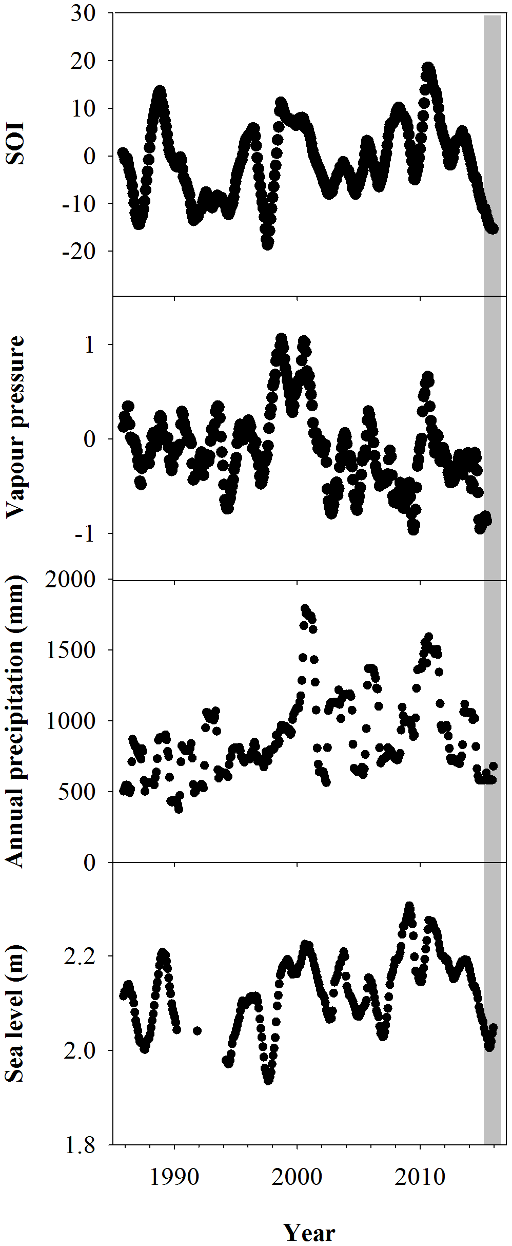
Figure 2 Climate observations from the south-eastern Gulf of Carpentaria, Australian (Jones et al., 2009; Harris et al., 2017; Bureau of Meteorology, 2019). The grey bar represents the period during which the dieback event occurred.

3.2 Wood samples and ages

The ages of A. marina ranged from 15±2 to 34±2 years (Table 1). On average, the trees in the living and dead mangrove forests were 21±4 and 34±1 years old respectively. Tree growth rates that were de-trended to negative exponential growth had no trends over time in either the living or dead mangrove areas (Table 1).

Table 1 Summary of radiocarbon ages and growth rates (deviation from negative exponential growth) for all wood samples taken from dead and living mangrove areas in the Gulf of Carpentaria, Australia.

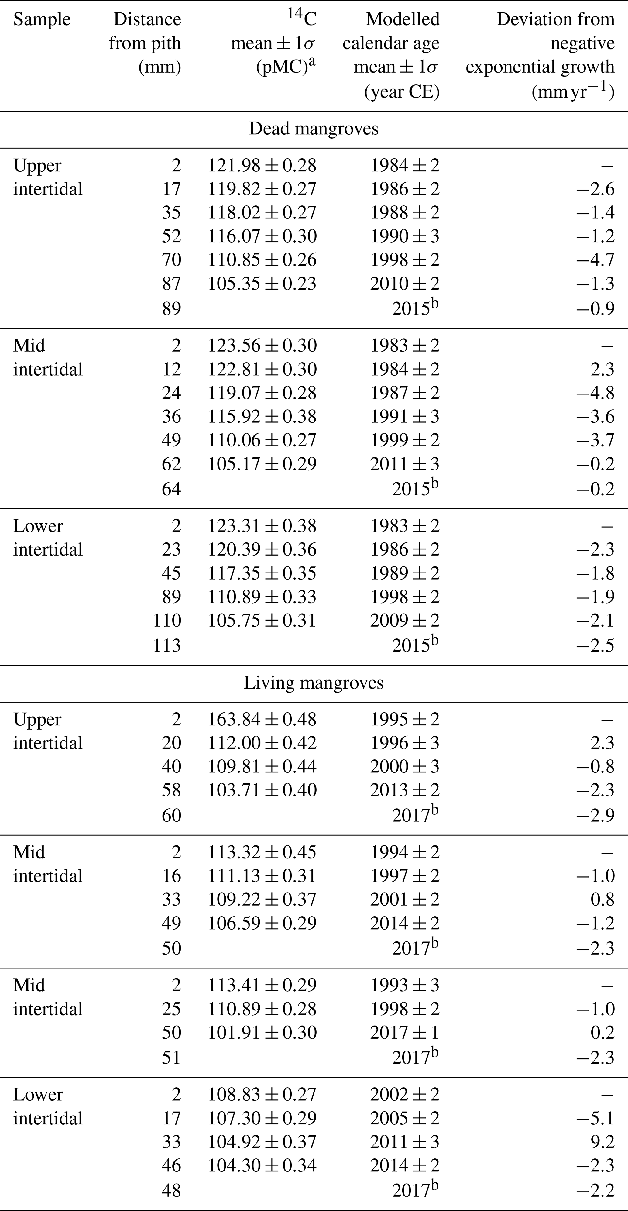
^a Measured ¹⁴C content is shown in percent modern carbon (pMC; Stuiver and Polach, 1977).
^b Year of collection of A. marina samples.

3.3 Fe in wood and sediment cores

Fe relative concentrations in all dead mangrove samples peaked at the time of mangrove mortality in late 2015–early 2016 (Fig. 3). In the living mangrove samples, Fe peaked in late 2015–early 2016 and then decreased in 2016 and 2017 to long-term average levels. Peak wood Fe concentrations in the upper, mid and lower intertidal areas of the dead mangrove samples were 40-, 90- and 30-fold higher respectively than their mean baseline concentrations (i.e. the average Fe concentrations in the sample prior to the dieback event). In the living mangrove area, peak wood Fe concentrations in the upper, mid and lower intertidal areas were 25-, 4- and 3-fold higher than their mean baseline concentrations respectively. In the dead mangrove area, Fe levels were similar from the upper to the lower intertidal zone (Fig. 3). In the living mangrove area, Fe was highest in the upper and mid intertidal zone and decreased in the lower intertidal zone. Itrax trends are plotted against ¹⁴C ages, and because tree growth rates change over time, Itrax data are not evenly distributed over time.

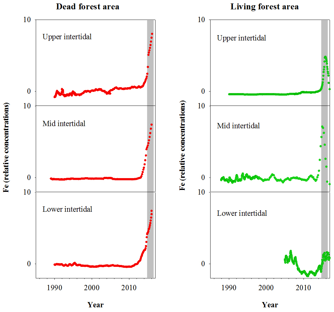
Figure 3 Fe relative concentrations in mangrove wood over time in living (green dots) and dead (red dots) mangroves from upper, mid and lower intertidal areas in the Gulf of Carpentaria, Australia. Grey areas indicate the dieback event.

Significant correlations with no time lag were found between Fe in wood and vapour pressure, rainfall, sea level and Southern Oscillation index (SOI; Fig. 4). All climate variables were strongly correlated with the SOI; therefore, we could not separate the influence of individual climate variables on wood Fe. In the dead and living mangrove areas, the strongest correlations with Fe occurred with no time lag (Fig. 4).

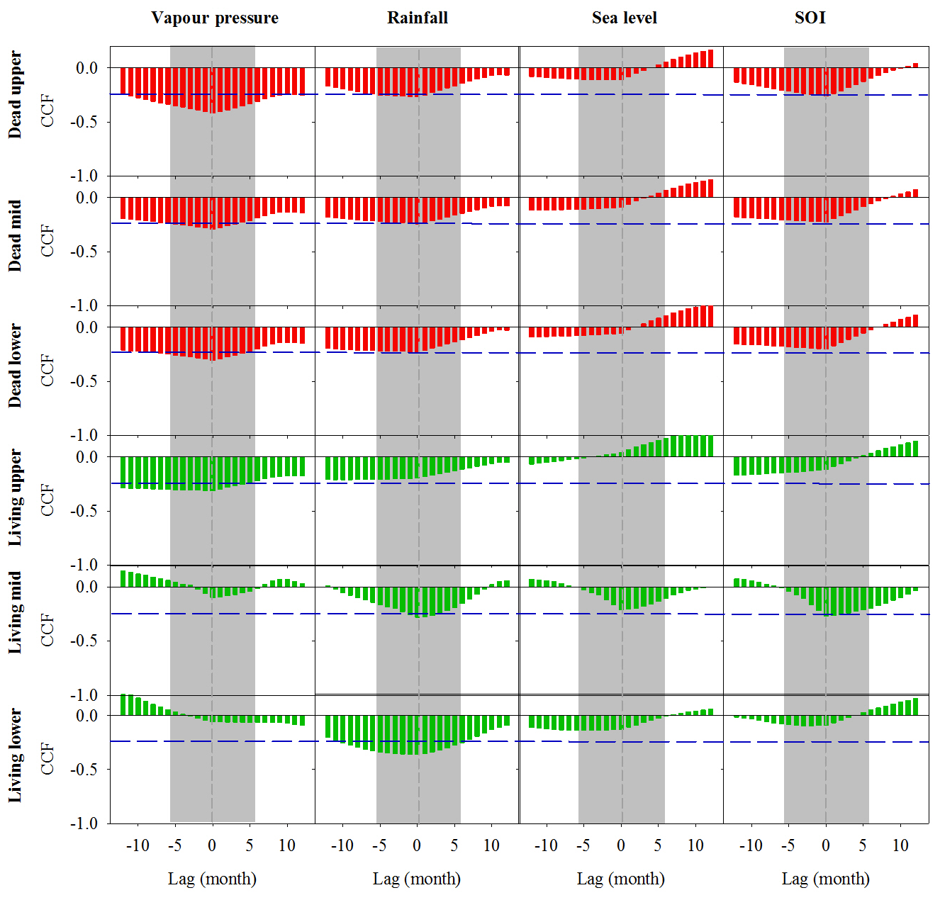
Figure 4 Cross-correlation function (CCF) between Fe in wood samples and climate data at a 1-month resolution over a 12-month period prior to and following dieback. Wood samples are from the upper, mid and lower intertidal zones of the dead (red) and living (green) mangrove areas. Blue horizontal dashed lines indicate P<0.01 with n=125. Grey dashed vertical lines at zero lag indicate the dieback period, and the grey bar represents the period during which the dieback event occurred.

Sediment cores had a similar pattern of decreasing Fe with depth in the upper and lower intertidal areas as well as in living and dead mangrove areas (Fig. 5a). Dead mangrove areas were depleted in Fe by ∼32 % in the surface 50 cm and by ∼26 % in the surface 1 m relative to the respective living mangrove areas in both the upper and lower intertidal areas (Fig. 5b, c, d). Fe relative concentrations were significantly higher in living mangrove areas compared with dead mangrove areas (Mann–Whitney rank sum test, P<0.001 for all depths).

Figure 5 (a) Fe relative concentrations in sediment cores to 2 m depth from the upper and lower intertidal areas of living (green) and dead (red) mangroves in the Gulf of Carpentaria, based on Itrax analysis. Box plots of normalized Fe relative concentrations from sediment cores to depths of (b) 0.5 m, (c) 1 m and (d) 2 m. The central horizontal line represents the median value, the box represents the upper and lower quartiles, and the whiskers represent the maximum and minimum values excluding outliers, i.e. the black dots.

Chromium-reducible sulfur (CRS) absolute concentrations, which provide a proxy for pyrite concentrations in sediment cores, were also lower overall in the dead mangrove area compared with the living mangrove area – by 36 % in the upper and 38 % in the lower intertidal zones respectively (Fig. 6). Although these differences were not significant (Mann–Whitney rank sum test, P>0.05), they were very similar to Itrax Fe trends. In the upper intertidal zone, CRS concentrations generally increased with depth, whereas in the lower intertidal zone, CRS concentrations peaked from ∼10 cm below the surface in both dead and living sediment samples and then decreased with depth. Differences in CRS concentrations (in both the upper and lower intertidal zones) between the dead and living mangroves were most prominent in the upper ∼60 cm of each core and tended to converge at greater depths (Fig. 6).

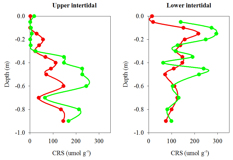
Figure 6 Chromium reducible sulfur (CRS) profiles (a proxy for pyrite) from sediment cores in dead (red) and living (green) mangrove areas in the Gulf of Carpentaria.

The water use efficiency (WUE) calculated from ¹³C decreased in all wood samples from 1983 to 2017 (Fig. 7a), suggesting increasing water availability in the study area. During the dieback event, median WUE values were higher in dead samples than in living samples, with the differences being more pronounced in the upper intertidal zones (Fig. 7b). The comparison of the WUE in dead and living mangrove samples suggests lower water availability in the dead mangrove area (Fig. 7b). However, the mean WUE values were compared from 1983 to 2017 and were not significantly different (t test, P=0.2) in dead and living mangrove areas. Groundwater salinity values were highest in the upper intertidal mangrove areas and lowest in the lower intertidal areas (Fig. 7c). Salinities were not significantly different in the living and dead forest areas (t test, P=0.913).

Figure 7 (a) Changes in the water use efficiency (WUE) over time in wood samples collected from the upper, lower and mid intertidal zone in living (green) and dead (red) mangrove areas. The grey bar represents the mangrove dieback event. Error bars are not visible due to the low error of individual samples. (b) Box plot of the water use efficiency in mangrove wood samples in dead and living mangrove areas in the upper, mid and lower intertidal zones. The sample size is greater than four from each wood sample. The central horizontal line represents the median, the box represents the upper and lower quartiles, and the whiskers represent the maximum and minimum values. (c) Box plot of groundwater salinity 8 months after the dieback event in the dead and living mangrove areas in the upper, mid and lower intertidal zones. The sample size is greater than three from each intertidal zone.

Normalized wood density values in the dead mangrove forest showed no change during the dieback event in the upper intertidal zone, but a decline in density values occurred in the mid and lower intertidal zones (Fig. 8). In the living mangrove area, declines in wood density values occurred in the upper and mid intertidal zones during the mortality event, but no variation in density occurred in the lower intertidal zone (Fig. 8).

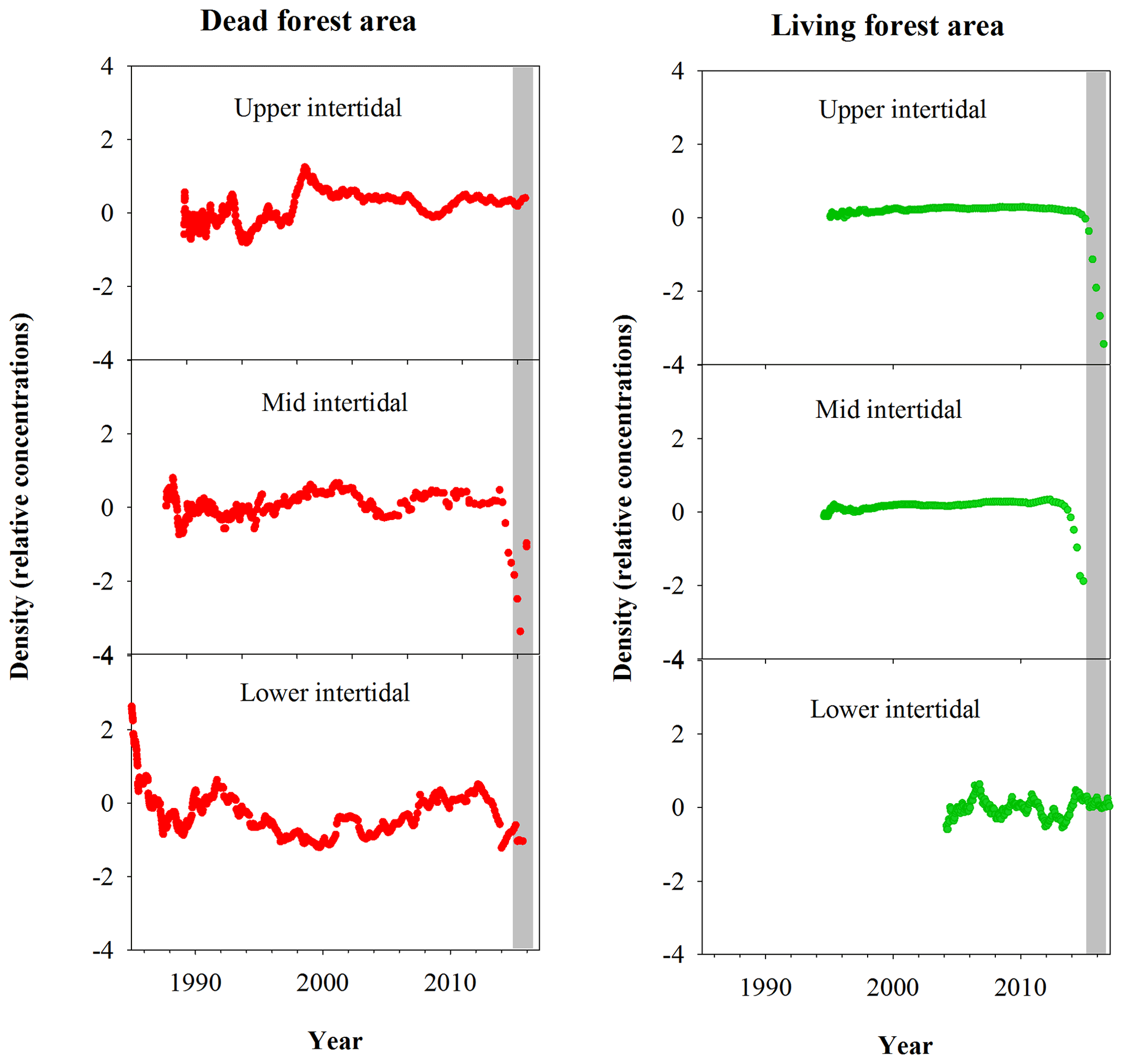
Figure 8 Normalized wood density (relative concentrations) in mangrove wood over time in living (green dots) and dead (red dots) mangrove areas of the Gulf of Carpentaria, Australia. The grey bar represents the time period of the dieback event.

4 Discussion

4.1 Evidence of differences in water availability between living and dead forest areas from dendrogeochemistry

Multiple lines of evidence from wood samples and sediment cores point to substantial differences in water availability between the dead and living mangrove areas. For example, Fe trends in wood (comparative Fe gain) and sediment samples (comparative Fe loss) within the dead mangrove zone (Figs. 3, 5, 6) both suggest the mobilization of bioavailable Fe as Fe²⁺. These observations are consistent with oscillations in sedimentary redox conditions, which are triggered by changes in water availability, promoting the mobilization of Fe – firstly as bioauthigenic pyrite is oxidized and then again during the reduction of Fe(III) oxide species when conditions return to being predominantly anaerobic (Fig. 9). Increased oxygen diffusion into sediments during the period of low water availability likely resulted in the oxidation of bioauthigenic pyrite, which transformed into aqueous and bioavailable Fe²⁺ (e.g. Fig. 9.2a; Johnston et al., 2011). With further oxidation, Fe²⁺ would likely have transformed into solid-phase Fe(III)oxides (Fig. 9.2b). Such Fe(III) oxides are highly reactive; thus, any subsequent short-term reduction (e.g. due to tidal inundation) would also result in remobilization of Fe as Fe²⁺ (Fig. 9.2c). The fact that the trends in Fe that were observed in wood and soil samples were not observed for other elements analysed by Itrax supports the hypothesis that Fe trends were likely related to pyrite oxidation and/or redox oscillations (Figs. A1, A2).

The most probable cause of a shift from reducing to oxidizing conditions in the sediment is a reduction in water content (Keene et al., 2014) associated with the intense El Niño of 2015–2016 and the related low sea levels and annual rainfall (Fig. 2). Trends in wood density, mangrove growth rate and water use efficiency also reveal distinct differences in water availability between dead and living forest areas. Lower water availability in the dead mangrove forest area was also evident in the lower plant growth rates and higher plant water use efficiency. Mangrove plant isotope data at the same sites from a study by Harada et al. (2020) also show a similar trend: more enriched ¹³C values in the dead mangrove zone.

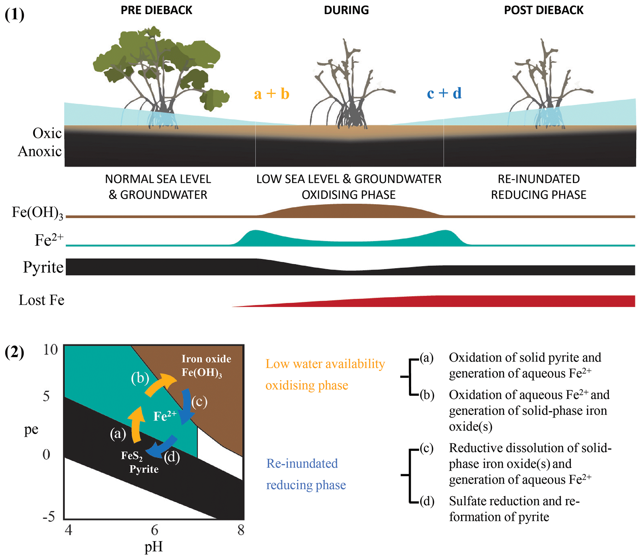
Figure 9 Conceptual diagram of Fe speciation under different sediment redox and pH conditions as well as (1) how speciation changes would be influenced by sea level and groundwater. Under initially elevated redox conditions due to low water availability (2) pyrite oxidation causes Fe transformation to (a) bioavailable Fe²⁺ and (b) particulate Fe(OH)₃ followed by the eventual re-establishment of normal water availability and reducing conditions as well as (c) the consequent reduction of Fe(OH)₃ and the generation of Fe²⁺ followed by (d) the sequestration of Fe(II) species via pyrite reformation.

4.2 Fe in wood

The elemental composition of wood samples suggest that the mangrove forest experienced sharp changes in sediment geochemistry during the dieback phase (Fig. 3). This is consistent with low sea levels and low rainfall (and likely groundwater) reducing soil water content, leading to the oxidation of Fe sulfide minerals and the release of Fe²⁺ (Fig. 9.2a). The Fe peaks in the dead mangrove area at the time of tree mortality were 30- to 90-fold higher than baseline Fe (the mean Fe concentration in the sample prior to the dieback event).

In the living mangrove area, an Fe peak 25-fold higher than baseline Fe was observed in the upper intertidal zone (Fig. 3). In the mid and lower intertidal areas of the living mangroves, Fe peaks were 4- and 3-fold higher than baseline values respectively. In all living wood samples, Fe subsequently decreased after the dieback event, suggesting that Fe in new wood growth was diminished in association with a return to sustained reducing sediment conditions and a concomitant attenuation in porewater Fe²⁺ availability (Fig. 9.2d).

Records of all climate variables are in the resolution of months, but the chronology of Fe (based on ¹⁴C dates) is in years. Therefore, we used time lag analysis to examine relationships between climate variables and Fe over a 2-year period (Fig. 4). Fe wood concentrations were significantly correlated with both rainfall and vapour pressure in the dead and living forest areas (Fig. 4). However, because all climate variables were strongly correlated with each other, we could not separate the relationships between individual climate drivers and Fe trends. We speculate that the combination of the low availability of fresh groundwater and low sea levels during the strong El Niño event of 2015–2016 are key drivers of the sediment redox conditions, as reflected in wood Fe trends.

Considering the extreme increases in Fe concentrations observed in the wood samples during the dieback event, it is plausible that Fe toxicity could have contributed to mangrove mortality. However, we cannot fully test this hypothesis in this study and are unaware of research testing the toxicity of Fe in A. marina at highly elevated concentrations of bioavailable Fe²⁺. Alongi (2010) found that Fe toxicity occurred in some mangrove species at high concentrations (100 mmol m² d⁻¹ of water-soluble Fe-EDTA) that were approximately 2-fold higher than the Fe supply for maximal growth. However, A. marina (the dominant species affected by the dieback at the study site) appear relatively resilient to high porewater Fe²⁺. For example, Johnston et al. (2016) observed no A. marina mortality at porewater Fe²⁺ concentrations of 7- to 15-fold above normal in a mangrove forest impacted by acid sulfate drainage. Considering that other mangrove species are affected by Fe toxicity at 2-fold the optimal Fe availability, it is possible that a 30- to 90-fold increase in Fe could have been an additional stressor to mangroves already stressed by low water availability.

While our observations suggest that complex sedimentary redox conditions occurred in dead-zone mangrove sediments during the dieback event, linking drought and low sea levels to porewater Fe concentrations requires further investigation. For example, crab burrows and root systems can induce conditions that increase O₂ diffusion into sediments and, thus, influence Fe²⁺ mobility over tidal cycles (Nielsen at al., 2003; Kristensen et al., 2008). Localized Fe(III) oxide dissolution can also occur in redox or pH micro-niches and under suboxic conditions (Fabricius et al., 2014; Zhu et al., 2012). Further research on the mechanisms of bioavailable Fe release and the thresholds for Fe toxicities in A. marina is required to clearly understand the impacts of porewater Fe on mangrove forests.

4.3 Fe in sediments

Sediment cores also displayed considerable differences in down-core Fe profiles between living and dead mangrove areas (Fig. 5a, b). Normalized Fe concentrations were lower in the upper 1 m of sediments in the dead mangrove area compared with the living, but they were very similar in sediments deeper than 1 m (Fig. 5a, b). Similar trends were also observed in CRS (a proxy for pyrite, FeS₂) sediment core profiles, which have ∼40 % lower FeS₂ concentrations in the dead mangroves in the upper 60 cm of the profile compared with the living mangrove sediments (Fig. 6). The fact that differences in down-core trends in Fe are most prominent in the upper parts of the sediment cores is consistent with decreases in water availability being more confined to the upper parts of the sediment profile, whereas deeper sediments are more likely to have remained fully saturated.

Although mangrove sediment conditions are typically highly heterogeneous (Zhu et al., 2006; Zhu and Aller, 2012), the sediment core results are broadly consistent with the wood data. The apparent mobilization of Fe (loss from sediment and uptake in wood) was not observed in other elements (Figs. A1, A2). Sediment Fe:Mn ratios in Itrax data displayed no clear differences between living and dead mangrove areas. These similarities may be because the sediment cores were taken after the dieback period when sediment geochemistry conditions returned to normal. Trends in Mn in the wood samples (Fig. A1) also show no clear differences between living and dead forest areas, and the Fe:Mn ratios in the wood Itrax data overwhelmingly reflect the Fe concentrations.

Sediment Fe losses, as implied by comparative Fe profiles (Figs. 3, 4, 6), also suggest a likely outwelling of Fe to the ocean. We estimate Fe outwelling by comparing FeS₂ concentrations in living and dead mangrove sediment cores based on the assumptions that (1) all Fe was originally in the form of FeS₂ and (2) tree Fe uptake is a minor loss pathway. The losses of Fe from the dead mangrove sediment would be equivalent to 87±163 mmol m² d⁻¹. The replication of CRS sediment cores (n=4) greatly limits the accuracy of our estimates. However, these fluxes are remarkably similar to short-term porewater-derived dissolved Fe fluxes (79±75 mmol m² d⁻¹) estimated for a healthy temperate salt marsh–mangrove system (Holloway et al., 2018) and provide some comparative restraint for our estimates.

If our sediment cores in dead and living mangroves were representative of changes within the entire dieback area (7400 ha), then total Fe losses from the dieback event could be equivalent to 87±163 Gg Fe. This loss is equivalent to 12 %–50 % of global annual Fe inputs to the surface ocean from aerosols (Jickells and Spokes, 2002; Fung et al., 2000; Elrod et al., 2004). As the surface ocean can be Fe limited, the consequences of Fe outwelling from a dieback event of this magnitude may have had an effect on productivity in the Gulf of Carpentaria.

4.4 Wood density, growth trends and water use efficiency

Clear decreases in the normalized wood density were observed during the mangrove mortality event (Fig. 8). Similar to trends in wood Fe, the wood density values in the living and dead forest areas were correlated with climatic indicators (Fig. A3). In A. marina trees, the observed decreases in wood density likely indicate decreased growth; however, the annual-scale resolution of ¹⁴C ages prevented detection of this short-term change in our growth rate data. Therefore, these clear decreases in wood density prior to tree mortality are an indication of stress, as decreased growth rates of mangroves can be associated with decreased water availability (Verheyden et al., 2005; Schmitz et al., 2006; Santini et al., 2013), which is also directly related to increased salinity. Low rainfall conditions and increased temperatures increase both evaporation and evapotranspiration while reducing freshwater inputs (Medina and Francisco, 1997; Hoppe-Speer et al., 2013).

Interestingly, no decrease in density was observed in the upper intertidal area of the dead mangroves (Fig. 8), despite the clear increase in Fe during the dieback in this tree sample (Fig. 3). This suggests that no change in growth occurred prior to tree mortality, implying rapid mortality in this case. The upper intertidal area of the dead mangroves may have been living at the limit of its tolerance range with respect to water availability or salinity prior to the dieback, as suggested by extremely high groundwater salinities in the upper intertidal areas of dead and living mangrove forests 8 months after the dieback event (Fig. 7c). No decrease in wood density was observed in the lower intertidal area of the living mangroves, which is consistent with both variation in the concentration of Fe and tree growth rate data. Together, these data suggest that the lower intertidal area of the living mangroves was not exposed to the same conditions during the dieback event as areas in the dead mangroves higher in the intertidal zone (Figs. 3, 8, 9). These results suggest a gradient of water availability, from extremely low availability at the upper intertidal zone of the dead mangrove area to high or optimal availability at the lower intertidal zone of the living mangrove area. As the elevation profiles are similar in the dead and living mangrove areas in the lower and mid intertidal areas (Fig. 1), it is possible that the difference in Fe trends between the mangrove areas is associated with the influence of regional groundwater flows on sedimentary redox conditions.

Mean growth rates of trees in living (4.4±3.6 mm yr⁻¹) and dead (5.3±3.5 mm yr⁻¹) mangrove areas are similar to rates measured by Santini et al. (2013) in A. marina in arid Western Australia (4.1–5.3 mm yr⁻¹). However, there was ∼10-fold greater variability in the present study because samples were collected from the upper, mid and lower intertidal zone, whereas Santini et al. (2012) sampled from the lower intertidal zone only. De-trended growth rate data showed that no consistent differences in growth trends were identified between mangrove areas (Fig. 8). The lower intertidal sample of the living mangroves grew more quickly during the dieback, which may suggest optimal conditions during this time. This may be due to increased nutrient availability stemming from litterfall inputs of organic matter from nearby stressed trees. All other sampled trees show no indication of reduced growth prior to or during the mortality event (Table 1). We suggest that climatic conditions drove very low growth rates during the dieback event, as indicated by wood density data (Fig. 8) and previous studies that found low growth during droughts (Cook et al., 1977; Santini et al., 2013).

A significant difference in mean ¹³C and WUE between living and dead mangrove areas was observed in the upper intertidal zone (t test, P=0.02), but not in the mid or lower intertidal zones (Fig. 7b). This is consistent with the zonation of mangrove mortality which occurred predominantly in the upper intertidal areas (Duke et al., 2017). The consistent decrease in the WUE suggests that water availability has been increasing over time in all intertidal areas since the 1990s (Fig. 7a). This is supported by generally increasing precipitation since the 1980s (Fig. 2), which enhanced mangrove areas in the Gulf of Carpentaria prior to this dieback event (Asbridge et al., 2016). Therefore, climatic conditions were initially favourable over the plants lifetime, and trees may have been insufficiently acclimated to withstand drought and low soil water availability during the dieback. Overall, this highlights the important role of extreme climatic events in counterbalancing mangrove responses to gradual climate trends (Harris et al., 2018).

4.5 Differences in water availability between living and dead forest areas

We have no data to determine if regional groundwater availability was greater in living forest areas than in dead forest areas during the mangrove dieback. No significant difference was observed in groundwater salinities 8 months after the dieback. However, under normal sea level conditions (i.e. when groundwater samples were collected), tidal inundation is likely to be the predominant driver of groundwater salinities rather than groundwater flows. Duke et al. (2017) and Harris et al. (2017) provide strong evidence that water availability in the Gulf of Carpentaria was extremely low prior to and during the dieback event. In this study, we have been able to build on this work by exploring links between changes in sediment geochemistry and low water availability.

We eliminate elevation as a potential driver of water availability in living and dead forest areas. Tree mortality even occurred in the lower intertidal zone of the dead mangrove area which is at the same elevation as the lower intertidal zone of the living forest area (see the elevation DEM in Fig. 1c). As other potential water sources were comparable between the sites, differences in water availability were likely driven by groundwater availability. Groundwater flows have high spatial variability and have been demonstrated to be an important water source in mangroves from arid Australia. For example, Stieglitz (2005) highlights that the interrelationships between confined and unconfined aquifers in the coastal zone can result in localized differences in groundwater flows. High-resolution spatial analysis of groundwater salinities in living and dead forest areas during low sea level conditions would help to clarify how water sources may drive mangrove mortality.

4.6 Limitations

This study is inherently limited in its spatial extent. Thus, the differences in Fe between samples from living and dead mangrove areas may be due to causal factors beyond the scope of this study. However, the consistency of results from multiple methods and divergent sample types provides some confidence in the interpretation that recent changes in sediment geochemistry have occurred in association with extreme drought and low sea level events.

Our analysis benefited from the development of high-precision ¹⁴C dating of mangrove wood samples (with age uncertainties of 1–3 calendar years, 1σ; see Table 1) that rely on the atmospheric bomb ¹⁴C content resulting from above-ground nuclear testing mostly in the late 1950s and early 1960s (Hua and Barbetti, 2004). The complexity in the wood development of A. marina creates uncertainties (Robert et al., 2011). Secondary growth in A. marina is atypical, displaying consecutive bands of xylem and phloem which can result in multiple cambia (i.e. the tissue providing undifferentiated cells for the growth of plants) being simultaneously active (Schmitz et al., 2006; Robert et al., 2011). Furthermore, A. marina cambia display non-cylindrical or asymmetrical growth (Maxwell et al., 2018). These characteristics of A. marina atypical growth can influence our results, as there is variation within each stem.

As younger wood grows on the exterior of the tree, errors associated with the estimated ages do not introduce uncertainty in the direction of trends but decrease the ability to find correlated trends with climatic variables (Van Der Sleen et al., 2015). In spite of these uncertainties, the strong cross correlations displayed in Fig. 4, with minimal time lag, suggest that the dendrochronology results are robust and that climate variability drives long-term Fe cycling in the coastal mangroves of the Gulf of Carpentaria.

5 Summary and conclusions

Wood and sediment geochemical data from living and dead mangrove areas suggest that there were substantive differences in their comparative sediment redox conditions during the dieback event. Climatic data and patterns in Fe concentrations in wood and sediment samples suggest that sediment oxidation occurred in combination with unprecedented low sea levels and low rainfall. As the elevation of dead and living mangrove areas was very similar, we suggest that the difference in tree survival between areas was probably due to higher groundwater availability at the living site. Evidence of plant Fe uptake and losses of Fe from sediments are consistent with this hypothesized Fe mobilization associated with low water availability in sediments. The dieback event was likely a period of transitioning redox states in a heterogeneous sediment matrix, which resulted in areas of mangrove sediments with low water availability combined with porewaters enriched in bioavailable Fe (Fig. 9).

Our data suggest that extremely low water availability drove the mangrove dieback. However, mangrove dieback may also be associated with increased concentrations of bioavailable Fe²⁺ in porewaters that occurred during this time of low water availability. Estimated losses of Fe from sediments were consistent with the observed plant uptake and suggest Fe mobilization due to sediment oxidation (and subsequent reduction). This Fe mobilization may also have led to significant Fe inputs to the ocean.

This study supports climate observations suggesting that the Gulf of Carpentaria dieback was strongly driven by an extreme El Niño–Southern Oscillation (ENSO) event (Harris et al., 2017). Climate change is increasing the intensity of ENSO events and climate extremes (Lee and McPhaden, 2010; Cai et al., 2014; Freund et al., 2019) as well as increasing sea level variability (Widlansky et al., 2015), which is impacting on mangrove forests in arid coastlines (Lovelock et al., 2017). Therefore, this study builds on the premise that the dieback event was associated with climate change (Harris et al., 2018). Further research is necessary to understand the role of Fe in tree mortalities, to constrain potential Fe losses to the ocean and from sediments, and to understand thresholds for Fe toxicities in A. marina.

Appendix A

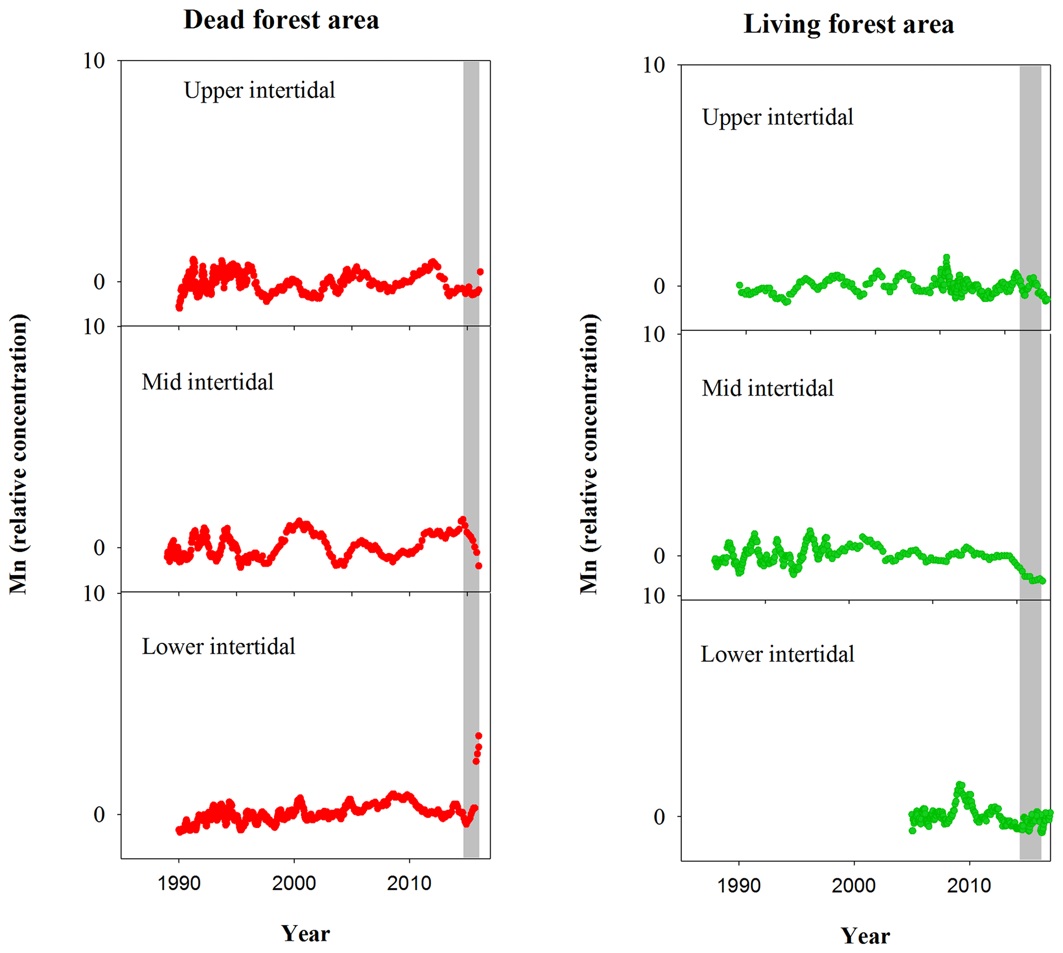
Figure A1 Normalized Mn relative concentrations in mangrove wood over time in living (green dots) and dead (red dots) mangroves from upper, mid and lower intertidal areas of the Gulf of Carpentaria, Australia. Grey areas indicate the dieback event.

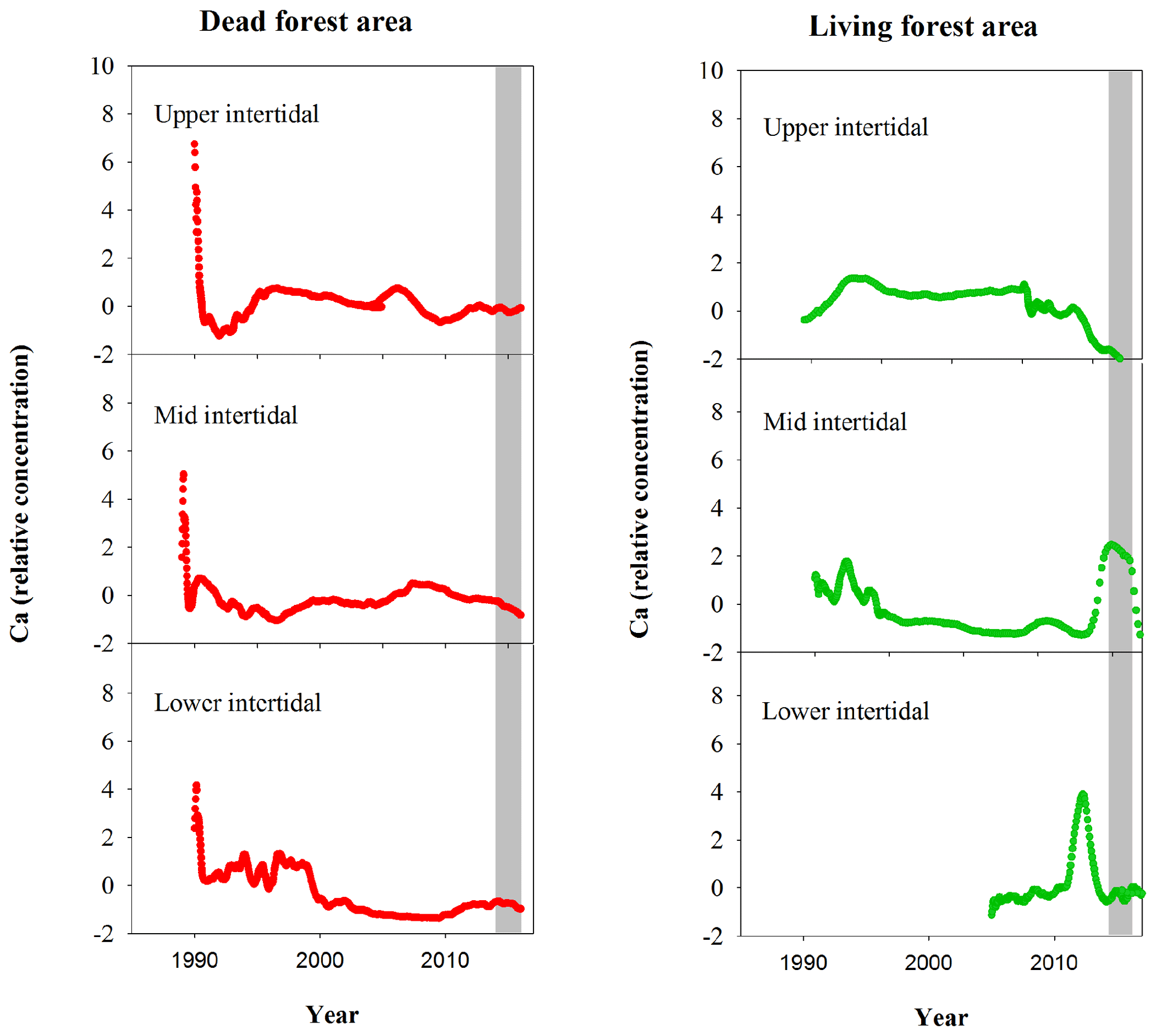
Figure A2 Normalized Ca relative concentrations in mangrove wood over time in living (green dots) and dead (red dots) mangroves from upper, mid and lower intertidal areas of the Gulf of Carpentaria, Australia. Grey areas indicate the dieback event.

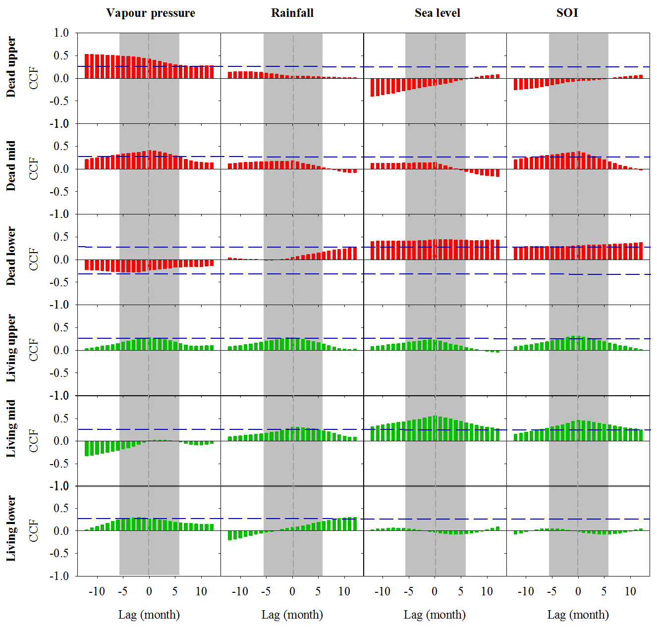
Figure A3 Cross-correlation function (CCF) analysis of the relationship between wood density and climate data over time at a 1-month resolution over a 12-month period prior to and following dieback. Wood samples are from the upper, mid and lower intertidal zones of the dead (red) and living (green) mangrove areas. Blue horizontal dashed lines indicate P<0.01 with n=125. Grey dashed vertical lines at zero lag indicate the dieback period.