the Creative Commons Attribution 4.0 License.
the Creative Commons Attribution 4.0 License.
 | 20 Oct 2020
Organic matter and sediment properties determine in-lake variability of sediment CO2 and CH4 production and emissions of a small and shallow lake
Leandra Stephanie Emilia Praetzel
Nora Plenter
Sabrina Schilling
Marcel Schmiedeskamp
Gabriele Broll
Klaus-Holger Knorr
Inland waters, particularly small and shallow lakes, are significant sources of carbon dioxide (CO2) and methane (CH4) to the atmosphere. However, the spatial in-lake heterogeneity of CO2 and CH4 production processes and their drivers in the sediment remain poorly studied. We measured potential CO2 and CH4 production in slurry incubations from 12 sites within the small and shallow crater lake Windsborn in Germany, as well as fluxes at the water–atmosphere interface of intact sediment core incubations from four sites. Production rates were highly variable and ranged from 7.2 to 38.5 µmol CO2 gC−1 d−1 and from 5.4 to 33.5 µmol CH4 gC−1 d−1. Fluxes ranged from 4.5 to 26.9 mmol CO2 m−2 d−1 and from 0 to 9.8 mmol CH4 m−2 d−1. Both CO2 and CH4 production rates and the CH4 fluxes exhibited a significant and negative correlation (p<0.05, ρ<−0.6) with a prevalence of recalcitrant organic matter (OM) compounds in the sediment as identified by Fourier-transformed infrared spectroscopy. The carbon / nitrogen ratio exhibited a significant negative correlation (p<0.01, ) with CH4 fluxes but not with production rates or CO2 fluxes. The availability of inorganic (nitrate, sulfate, ferric iron) and organic (humic acids) electron acceptors failed to explain differences in CH4 production rates, assuming a competitive suppression, but observed non-methanogenic CO2 production could be explained up to 91 % by prevalent electron acceptors. We did not find clear relationships between OM quality, the thermodynamics of methanogenic pathways (acetoclastic vs. hydrogenotrophic) and electron-accepting capacity of the OM. Differences in CH4 fluxes were interestingly to a large part explained by grain size distribution (p<0.05, ). Surprisingly though, sediment gas storage, potential production rates and water–atmosphere fluxes were decoupled from each other and did not show any correlations. Our results show that within a small lake, sediment CO2 and CH4 production shows significant spatial variability which is mainly driven by spatial differences in the degradability of the sediment OM. We highlight that studies on production rates and sediment quality need to be interpreted with care, though, in terms of deducing emission rates and patterns as approaches based on production rates only neglect physical sediment properties and production and oxidation processes in the water column as major controls on actual emissions.
- Article
(2031 KB) - Full-text XML
-
Supplement
(630 KB) - BibTeX
- EndNote


Inland waters play an important role in the global carbon (C) cycle and contribute significantly to natural emissions of the greenhouse gases carbon dioxide (CO2) and methane (CH4) (Cole et al., 2007; Battin et al., 2009; Bastviken et al., 2011; Raymond et al., 2013; Regnier et al., 2013). Lakes and reservoirs are estimated to emit in total 0.32–0.39 Pg C of CO2 and 0.58 Pg C (CO2 eq.) of CH4 year−1 (Cole et al., 2007; Bastviken et al., 2011; Raymond et al., 2013), but especially small lakes (<0.1 km2) have previously been underestimated regarding their spatial expansion and, therefore, their contribution to global greenhouse gas emissions (Downing, 2010). Although small lakes account for of the total lake area and cover less than 1 % of the global land surface, they contribute 35 % of the CO2 and 72 % of the CH4 emissions from lakes worldwide (Downing et al., 2006; Holgerson and Raymond, 2016). Further, even though most lakes are found in boreal zones, the largest areas occur in lower latitudes around 50∘ (Verpoorter et al., 2014). In small lakes, due to their shallowness, shorter water residence times and smaller perimeter to volume ratios, metabolic processes and C turnover are much faster than in larger lakes, making small lakes potentially more susceptible to environmental and climatic changes (Wetzel, 1992; Downing, 2010).
Recently, many studies have shown that both CO2 and CH4 fluxes are highly variable both on spatial and temporal scales, but the majority of these measurements have been performed on larger lakes and are concentrated in boreal regions (Schilder et al., 2013; Wik et al., 2013; Bastviken et al., 2015; Natchimuthu et al., 2016, 2017; Spafford and Risk, 2018). Beyond that, few studies have examined greenhouse gas (GHG) production processes in the sediments or have attempted to link sediment GHG production to emissions. Nevertheless, anoxic sediments are important for whole-lake C cycling as the CO2 and CH4 produced there can be released through the water column to the atmosphere. To understand the spatial patterns of CO2 and CH4 emissions, it is, therefore, of interest to also understand CO2 and CH4 production processes in the sediment, as well as their major controls.
The amount of CO2 and CH4 produced in lake sediments relates to the degradability of the organic matter (OM) present, which depends primarily on its quality, the microbial biomass and enzyme activities (Updegraff et al., 1995; McLatchey and Reddy, 1998; Fenchel et al., 2012). While the origin and the degradation state of OM can be determined using carbon / nitrogen (C∕N) ratios, qualitative information about OM components can be determined via Fourier-transformed infrared (FTIR) spectroscopy. The latter technique can, therefore, further provide information about the origin and degree of decomposition of OM (Meyers, 1994; Broder et al., 2012; Biester et al., 2014; Li et al., 2016). The prevalence of different OM compounds leads to specific features in FTIR spectra as functional moieties have wavelength-specific absorption maxima (Niemeyer et al., 1992; Cocozza et al., 2003). Artz et al. (2008) compiled a range of functional moieties that are used to characterize OM in peat soils, which is also applicable to OM in general. While polysaccharides and proteins are preferentially degraded by microorganisms, aliphatic (e.g., waxes) and aromatic compounds (e.g., lignin) are more recalcitrant (due to their molecular structure) and, therefore, residually accumulate in the anoxic sediment (Fenchel et al., 2012; Tfaily et al., 2014).
In anoxic sediments, CO2 and CH4 are produced during the breakdown of OM over a cascade of microbially mediated processes. After the cleavage of complex organic polymers, resulting monomers are fermented, which mainly produce hydrogen (H2) and low molecular weight organic compounds (e.g., acetate). The low molecular weight compounds are further oxidized to CO2, and H2 to H2O upon consumption of electron acceptors (EAs; nitrate, sulfate, ferric iron or humic substances). Only subsequently is CH4 production as the final step of terminal electron-accepting processes initiated after all other thermodynamically more favorable EAs are depleted (Achtnich et al., 1995; Blodau, 2011). CH4 is mainly produced via two different pathways, the acetoclastic pathway and the hydrogenotrophic pathway, for which either acetate is the substrate (acetoclastic; Reaction R1) or H2 is the substrate and CO2 is the EA (hydrogenotrophic; Reaction R2) (Conrad, 1999; Whiticar, 1999). Values for for these terminal electron-accepting processes and methanogenesis can be calculated from standard formation energies in aqueous state, as listed in Stumm and Morgan (1995) and Nordstrom and Munoz (1994):
Several studies have shown that in anoxic wetland and marine sediments rich in labile organic compounds, the acetoclastic pathway dominates. With increasing recalcitrance, the hydrogenotrophic pathway becomes more important as acetate, being the direct precursor of CH4, is depleted (Schoell, 1988; Hornibrook et al., 1997; Miyajima et al., 1997). As suggested by Lojen et al. (1999), the OM quality in lake sediments might thus be responsible for seasonal changes in the dominant CH4 pathway.
Whereas many studies have shown that inorganic EAs can suppress methanogenic activity (e.g., Yao et al., 1999; Fenchel et al., 2012), information on the role of humic substances as organic EAs remains scarce. In one study, Klüpfel et al. (2014) revealed that humic substances can be reduced and reoxidized at oxic–anoxic interfaces in peatlands, sediments or soils underlying water table fluctuations, and another study showed that in peat soils poor in inorganic EAs, the electron-accepting capacity (EAC) of OM represents the major control on CO2 and CH4 production (Gao et al., 2019). As sediments from the lake we investigated are also rich in OM, we wanted to verify whether the EAC and electron-donating capacities (EDC) of humic substances also play a vital role in explaining the spatial variabilities of CO2 and CH4 production in lake sediments. Although they are not subject to water table fluctuations, they might, in the upper parts of the sediments, be influenced by oxygen penetration from the water column due to a well-mixed water body, particularly in shallow lakes (Lau et al., 2016).
Overall, the amount of CO2 and CH4 produced, therefore, depends on either the availability and degradability of the OM itself, the presence of EAs, or the levels of H2 and acetate as substrates for methanogenesis (Segers, 1998; Conrad, 1999; Megonigal et al., 2003; Blodau, 2011; Fenchel et al., 2012).
Within lakes, the spatial distribution of OM and other sediment properties vary considerably in terms of their origin (terrestrial vs. aquatic), degradability, elemental geochemistry and grain size (Muri and Wakeham, 2006; Ostrovsky and Tęgowski, 2010; Tolu et al., 2017). Further, sediment grain size is an important factor for the evolution of CH4 bubbles in sediments (Ostrovsky and Tęgowski, 2010; Liu et al., 2018); for example, Liu et al. (2016) revealed that CH4 ebullition decreases with increasing shares of sand in lake sediments. Overall though, CH4 ebullition is thought to account for a large proportion (75 %) of CH4 emissions from lakes (Bastviken et al., 2011).
Until now, laboratory incubations of lake sediments were mostly conducted with samples from one or a few sites within one lake with a focus on comparing different lakes with each other rather than covering a high in-lake variability of production rates. Further, these studies emphasize temperature effects on production rates (Duc et al., 2010; Gudasz et al., 2010, 2015; Fuchs et al., 2016). Unlike in peat soils, where a broad range of process-based controls on CO2 and CH4 production has been studied, in small lakes, controls such as OM quality, the occurrence of alternative EAs, thermodynamic processes and sediment grain size have not or have only individually been systematically surveyed. To close this knowledge gap, we determined the magnitude and spatial variability of sediment CO2 and CH4 production in a small and shallow temperate lake in order to relate observed production patterns to measured OM and sediment characteristics, thermodynamics of methanogenesis, and water–atmosphere fluxes. To this end, we conducted slurry and intact sediment core incubations with sediment from the crater lake Windsborn in Germany. This site was chosen as a model system because it has a high sediment OM content (∼30 %), a very small catchment area, and no surficial in- or outflows, meaning minimal influence from the surrounding catchment.
We hypothesized (I) that CO2 and CH4 production vary spatially in the sediment, (II) that the variability in the production rates is reflected in the flux patterns; and (III) that the variation in production rates, methanogenic pathways and flux patterns can be explained by factors of OM degradability, availability of organic and inorganic EAs, and grain size distribution, or a combination of these factors.
2.1 Study site
The studied Lake Windsborn is a polymictic, small, shallow crater lake in the Volcanic Eifel, Rhineland Palatinate, southwest Germany, and is part of the Mosenberg volcano group (see Fig. 1) (LfU, 2013). The climate is temperate with a mean annual temperature of 8.3 ∘C and 931 mm precipitation (multiannual mean 1981–2010; DWD, 2019). Lake Windsborn is the only genuine crater lake north of the Alps. It emerged approx. 29 000 years ago after a volcanic eruption when the top of the volcano had been blasted away and the newly formed crater was subsequently filled with water (LfU, 2013). The present lake formed around 1850, after drainage of the lake and the partial removal of the peat from the lake bottom (Kappes and Sinsch, 2005). The lake is part of a conservation area that was established in 1927 (Kappes and Sinsch, 2005). From 1950 until the 1990s, the lake was used as a fishing ground and was, therefore, stocked with fish and limed (LfU, 2013). The lake is nearly circular and surrounded by a 20 to 30 m high rampart which consists of an alternation of red-brown ashes, slag and lapilli from the eruption. Therefore, it has a very small catchment of only about 8 ha compared to the lake surface of 1.41 ha, and it has no surficial in- and outflows and is only fed by groundwater and precipitation (LfU, 2013; Meyer, 2013). The maximum lake depth varies between 1.3 and 1.7 m (Kappes and Sinsch, 2005). The area is underlain by Devonian quartzite (Kampf, 2005).
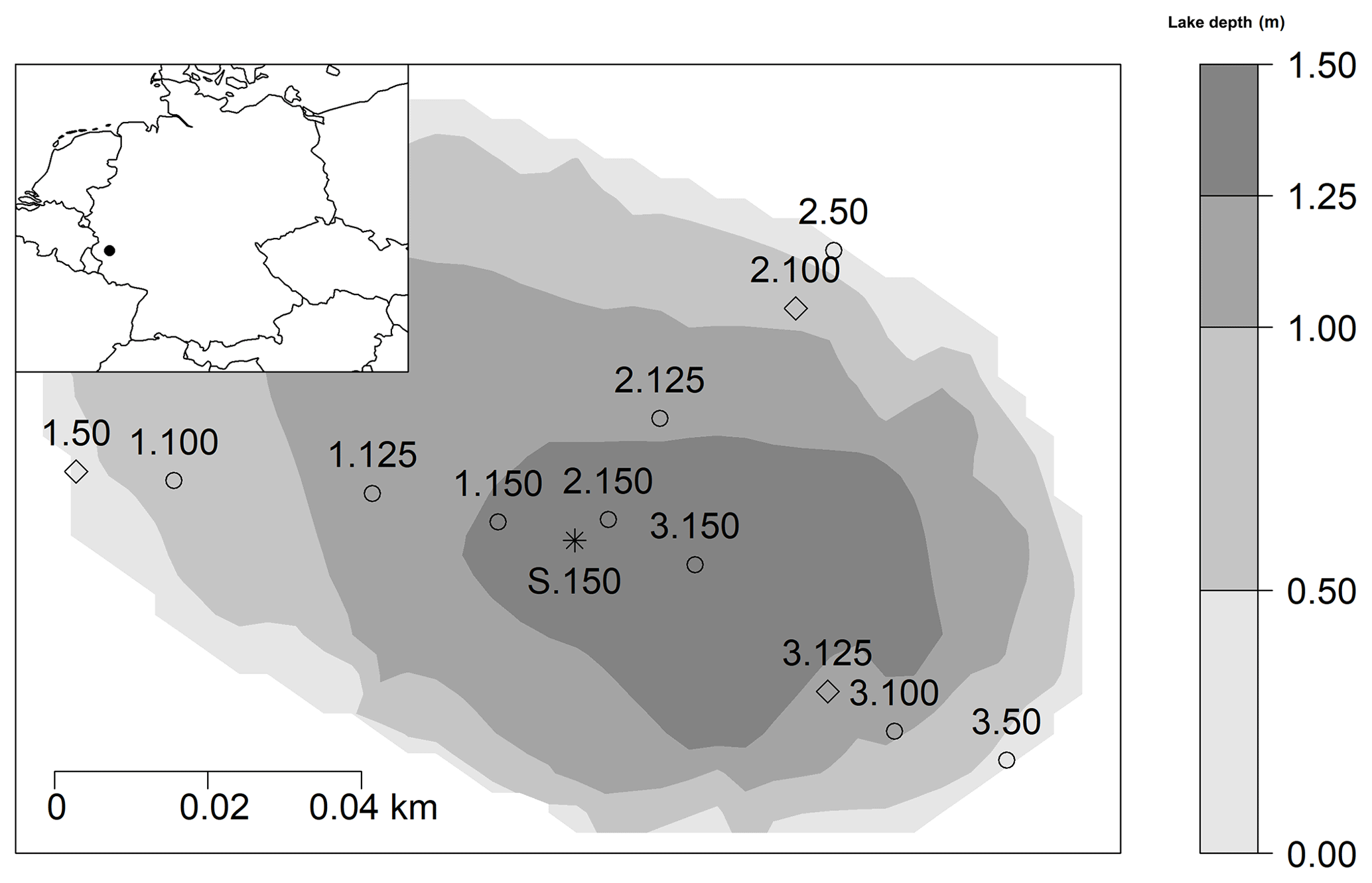
Figure 1Location of the study area in Germany (black spot on the map top left) and 13 sampling sites within Lake Windsborn. Diamonds: sampling sites for slurry incubations and intact sediment core incubations. Circles: sites for slurry incubations only. Asterisk: site for intact sediment core incubation only (reference for 1.150, 2.150 and 3.150). Depths were interpolated by bivariate linear interpolation. Numbers 1, 2 and 3 refer to the transect number from the lake shore to center, and numbers 50, 100, 125 and 150 indicate lake depth category (50: <50 cm; 100: 50–100 cm; 125: 100–125 cm; 150: 125–150 cm).
The lake's shoreline is vegetated with Carex rostrata, Comarum palustre and Menynanthes trifoliata, all indicating poor nitrogen (N) supply (Ellenberg et al., 2001). At the northwestern riparian zone, there is a quaking bog mainly dominated by Sphagnum spec. whose expansion will slowly lead to the silting up of the lake. Lake Windsborn was previously considered humic-oligotrophic, but, in the early 1990s, it transitioned to a eutrophic lake, and now it is slowly recovering from human impacts and nutrient input (Kappes et al., 2000). During our measurement campaigns in 2017 and 2018, the lake exhibited partly meso- and eutrophic features as shown in Table 1.
Table 1Selected lake water characteristics measured in Lake Windsborn in 2017 and 2018: pH, conductivity (cond.), dissolved oxygen (O2), chlorophyll α (Chl. α), dissolved organic carbon (DOC), total dissolved nitrogen (TN), chloride (Cl), calcium (Ca), iron (Fe), potassium (K), magnesium (Mg), sodium (Na), phosphorous (P) and sulfur (S).

2.2 Slurry incubations
2.2.1 Sampling and preparation of slurry incubations
For the slurry incubation experiment, samples were taken on three occasions (in March, April and May 2018) from 12 of the 13 sampling sites within the lake from three transects covering multiple water depths (<50, <100, <125 and <150 cm) (see Fig. 1). On each sampling date, 4 of the 12 sampling sites were chosen randomly as it was not possible to set up the experiment with all samples at once. At the sampling dates, measured air, water and sediment temperatures at the sampling dates were 7.7, 5.6 and 5.2 ∘C (March), 13.8, 15.1 and 10.1 ∘C (April), and 23.9, 23.6 and 13.8 ∘C (May), respectively. Sediment samples were taken in duplicates with a gravity corer (UWITEC, Mondsee, Austria) from a boat in 60 cm long PVC tubes and transported in an insulated box at ∼5 ∘C. The next day, sediment cores were cut with a core cutter in the laboratory in segments of 5 cm thickness (0–5 and 5–10 cm sediment depth). Duplicate samples were homogenized, and then 20 g of each sediment was filled into 120 mL crimp vials containing 20 mL lake water, after which the vials were closed with a butyl rubber stopper and aluminum crimp cap. Samples were flushed with N2 for 30 min in order to remove any remaining oxygen from the water and headspace, and then they were preincubated for one week so they were fully anoxic. They were again flushed with N2 prior to the actual incubation. Slurry incubations were set up in triplicates and maintained at 25 ∘C (corresponding to maximum measured in situ sediment temperatures in summer 2018) in the dark. During each run, one set of parallel samples was incubated at 10 ∘C in order to determine a Q10 value for CO2 and CH4 production rates.
The remaining sample material was freeze-dried (Alpha 1–4 LDplus, Christ, Osterode, Germany), ground with a ball mill (Mixer Mill MM 400, Retsch, Haan, Germany) and used for solid-phase analyses, as outlined below.
2.2.2 Sediment OM quality
Freeze-dried and ground sediment samples were analyzed for total C and N concentrations and stable isotopes using isotope-ratio mass spectrometry (IRMS; EuroVector EA3000 coupled with Nu Instruments Nu Horizon, HEKAtech, Wegberg, Germany) and for OM components using FTIR spectroscopy (Cary 670 FTIR Spectrometer, Agilent, Santa Clara, USA).
For IRMS, 5 mg of sample was weighed out into a tin cup, together with 4 mg of vanadium pentoxide (V2O5). The combustion and reduction furnaces were set to 1000 and 650 ∘C, respectively, and the resultant gaseous compounds were quantified by IRMS. Results are provided in percent (%) by mass for C and N contents (precision <1 % for C and <0.1 % for N) and in per mill (‰) vs. VPDB/AIR (Vienna Pee Dee Belemnite; atmospheric N2) for C and N isotopic signatures (precision <0.05 ‰ for 13C and <0.5 ‰ for 15N). For isotope analyses, appropriate certified reference materials were used: IAEA 600 (δ13C = −27.77 ‰; δ15N = 1.0 ‰) and BBOT (2.5-Bis-(5-tert.-butyl-2-benzo-oxazol-2-yl)thiophen; HEKAtech, Wegberg, Germany), birch leaf, wheat flour and sorghum flour standards (IVA Analysetechnik e. K., Meerbusch, Germany) as working standards covering a range of −27.5 ‰ to −13.68 ‰ for 13C and −0.6 ‰ to 2.12 ‰ for 15N.
Functional groups of OM compounds were identified by FTIR spectroscopy. For this purpose, 2 mg of freeze-dried sample was ground together in a mortar with 200 mg KBr (potassium bromide), pressed into 13 mm pellets and analyzed. Each sample was scanned from 599 to 4000 cm−1 with a resolution of 2 cm−1 and was baseline corrected. Distinct peaks at specific wavelengths were assigned to functional groups according to Artz et al. (2008) and normalized to the peak intensity at 1031–1035 cm−1 (indicative of polysaccharides) in order to obtain intercomparable peak ratios of functional moieties in all samples, as FTIR spectra only provide information about the relative abundance of certain functional moieties in one sample.
2.2.3 CO2 and CH4 production rates from slurry incubations
Potential CO2 and CH4 productions rates were determined by measuring the increase in concentration of CO2 and CH4 in the incubation vials over time. Concentrations were obtained by analyzing the headspace at the beginning of the experiment (t0) and after 1, 3, 8, 11, 14 and 18 d (t1–t6). Samples were taken from the vial with a 10 mL polypropylene syringe equipped with a three-way stopcock and a 0.6 mm needle. Before each sampling, the pressure inside the vial was determined with a pressure sensor (GMH 3110, Greisinger, Regenstauf, Germany), and the syringe was flushed three times with N2. Then 2 mL of N2 was left in the syringe before the needle was stabbed through the vial's stopper, whereby the N2 was added to the headspace and mixed, and, subsequently, 2 mL of the sample was taken from the vial so that the volume inside the vial remained constant. The gas samples were analyzed for CO2 and CH4 concentrations with a gas chromatograph (8610 GC-TCD/FID, SRI Instruments, Torrance, USA) equipped with a flame ionization detector (FID) and methanizer to simultaneously measure CO2 and CH4. Before every sampling day, the gas chromatograph was calibrated with standard gas mixtures of known concentrations (CO2: 385, 5000 and 50 000 ppmV; CH4: 5, 1000 and 50 000 ppmV).
First, measured concentrations (in ppmV) were pressure corrected and converted using the ideal gas law:
where n is the amount of substance (in mol), p is the gas partial pressure (in atm), V is the headspace volume (in L), R is the ideal gas constant (0.082 L atm mol−1 K−1) and T is the laboratory temperature (in K).
Total CO2 and CH4 concentrations in the gas and water phase in the incubation vials were calculated from headspace concentrations using Henry's law:
where c is the concentration in the water phase (in mol L−1), Kh is the temperature-dependent Henry constant (CO2, 25 ∘ = 0.0339 mol L−1 atm−1; CH4, 25 ∘C = 0.00129 mol L−1 atm−1; Sander, 2015) and p is the gas partial pressure (in atm).
Moreover, CO2 concentrations were pH corrected in order to obtain pH-independent values for total CO2 concentrations using the Henderson–Hasselbalch equation and equilibrium constants according to Stumm and Morgan (1995):
where is the pH-corrected CO2 amount (in mol) and nwater is the calculated amount of CO2 in the water phase (in mol).
Finally, production rates were calculated by linear regression (R2>0.8 for CO2 and R2>0.9 for CH4) from concentration change in gas and solute phase over time.
To evaluate the effect of temperature on CO2 and CH4 production, we calculated Q10 values, describing the relative increase of production rates with an increase in temperature of 10 K (Fenchel et al., 2012):
where R2 is the production rate at T2 (25 ∘C) and R1 is the production rate at T1 (10 ∘C).
2.2.4 Thermodynamics and methanogenic pathways
In order to calculate the thermodynamic energy yield for hydrogenotrophic and acetoclastic methanogenesis, we measured H2 concentrations at the beginning, after 8 d (t3) and at the end of the experiment, and we measured acetate concentrations at the beginning and at the end of the incubation. The thermodynamic energy yield, expressed as Gibbs free energy, was calculated using the Nernst equation and total dissolved and gaseous concentrations of educts and products in the incubation vials as described in Beer and Blodau (2007):
By calculating the Gibbs free energy (ΔGr), it is possible to evaluate whether these processes are feasible under given conditions. In order for each reaction to occur, a theoretical threshold of to −25 kJ mol−1 had to be exceeded (Schink, 1997; Conrad, 1999; Blodau, 2011).
For H2 concentration measurements, 2 mL of sample was taken from the incubation headspace with a syringe and needle and replaced with the same amount of N2. Samples were analyzed with a reduction gas detector (RGD) hydrogen and carbon monoxide analyzer (ta3000R Gas Analyzer, Ametek, Pittsburgh, USA) that was calibrated with gas standards of 5, 25 and 50 ppmV H2. Measured H2 concentrations were corrected for pressure and converted into dissolved concentrations using Henry's law (Kh(H2, 25 ∘C) = 0.00078 mol L−1 atm−1; Sander, 2015) analogous to CO2 and CH4.
Acetate concentrations were determined through ion chromatography with chemical suppression (883 Basic IC plus, Metrohm, Filderstadt, Germany; A Supp 5 column, Metrohm, Filderstadt, Germany). Aqueous samples were filtered with 0.45 µm nylon plus glass microfiber syringe filters (Simplepure, BGB Analytik, Rheinfelden, Germany) and kept frozen at −21 ∘C until analysis.
2.2.5 Alternative EAs
To quantify alternative EAs that could support anaerobic respiration and potentially suppress methanogenesis in anoxic incubations, we measured nitrate (), sulfate (), ferric iron (Fe3+), and the EAC and EDC of the OM (EACOM and EDCOM) at the beginning and the end of the slurry incubation.
As the analysis of EACOM and EDCOM is only possible on finely ground materials, thus providing potential capacities rather than true in situ capacities, we set up a second set of slurry incubations for a sediment depth of 0–5 cm with samples from 10 sites (all except 3.50 and 3.100) using 0.4 g of the freeze-dried sediment material and 100 mL of Milli-Q® water. Slurry incubations were set up in six replicates, flushed with N2, preincubated and stored analogously to the first set of slurry incubations. Samples were analyzed at the beginning and at the end of the experiment since at every sampling occasion, three of the replicates had to be sacrificed (destructive sampling). Prior to analysis, samples were transferred into a glovebox (O2 <1 ppm; Innovative Technology, Amesbury, USA) to avoid alteration of the samples' redox state.
EACOM and EDCOM were measured using chronoamperometry (CHI1000C, CH Instruments, Austin, USA) by mediated electrochemical reduction (MER) and oxidation (MEO) (Aeschbacher et al., 2010; Klüpfel et al., 2014). The cell consisted of a cylindrical glassy C working electrode, a platinum wire counter electrode in a ceramic glass frit and an Ag∕AgCl reference electrode. Cells were filled with 10 mL of 0.01 M MOPS and 0.1 M KCl buffer to stabilize the pH at 7 and were continuously stirred during measurement. To facilitate electron transfer, organic mediators were added to the buffer: 180 µL DQ (diaquat dibromide monohydrate; Sigma-Aldrich) for MER and 180 µL ABTS (2,2′-azino-bis(3-ethylbenzthiazoline-sulfonic acid), Sigma-Aldrich) for MEO at a potential of V and V, respectively (reported vs. the standard H2 electrode but experimentally measured vs. the Ag∕AgCl reference electrode). To determine the electron transfer, 100 µL of suspended samples were added to the buffer solution (Lau et al., 2015) which resulted in an increase of the current, recorded as a peak in the analysis software. After ∼30 min, when the baseline was reached again, the next sample was added to the cells. Samples were analyzed in duplicate. The electron transfer was calculated with the Nernst equation and normalized to the C content in the samples (Lau et al., 2015):
where V is the sample volume (in µL), F is the Faraday constant (96 485 A sec/mol e−) and C is the C content (in mg L−1) (EACOM and EDCOM in µmol e− gC−1; peak area in µA seconds).
EACOM and EDCOM had to be corrected for either ferric iron (Fe3+) or ferrous iron (Fe2+) and sulfide (S2−) concentrations, respectively, since with the applied potential, Fe3+ would be reduced and Fe2+ and S2− would be oxidized (Lau et al., 2015; Agethen et al., 2018).
Fe2+, Fe3+ and S2− were determined colorimetrically (Gilboa-Garber, 1971; Tamura et al., 1974) with a spectrophotometer (Cary 100 UV-Vis, Agilent, Santa Clara, USA). Because 1,10-phenanthroline can only detect Fe2+, the Fe3+ in the samples was reduced to Fe2+ with 10 % ascorbic acid. Ferric iron was thus determined as the difference of total Fe and ferrous iron in the samples.
and concentrations were determined with ion chromatography (IC), as described above. For this purpose, samples were filtered with a 0.45 µm syringe filter, added into micro-centrifuge tubes, retrieved from the glovebox and stored frozen at −21 ∘C until analysis.
Total EAC (EACtot) was calculated as the sum of EACOM and EACinorg (EAC from nitrate, sulfate, ferric iron) considering the respective amounts of electrons transferred during the main pathways of dissimilatory reduction, i.e., assuming a reduction of to N2, of to S−2 and of Fe3+ to Fe2+ (Konhauser, 2009):
Assuming reversibility of electron transfer to and from OM, EACOM and EDCOM correlate with each other. If EACOM decreases, EDCOM increases equivalently as quinones are reduced to hydroquinones; in practice, values of EDCOM are potentially biased as MEO does not only capture EDCOM but may also irreversibly oxidize phenolic moieties, which are sensitive to the slightest changes in pH and potentials (Aeschbacher et al., 2011; Walpen et al., 2016, 2018). The discussion will, therefore, focus on EACOM data.
2.3 Intact sediment core incubations
2.3.1 CO2 and CH4 fluxes
To obtain ex situ CO2 and CH4 gas fluxes and estimate changes in sediment CO2 and CH4 stocks, intact sediment cores (PVC tubes, 60 cm length, 5.8 cm diameter) were taken in triplicate from 4 out of the 12 sites in November 2017 (1.50, 2.100, 3.125, S.150; see Fig. 1). S.150 was chosen as one site to represent sites 1.150, 2.150 and 3.150 from the same lake depth category. Sediment cores were transported cool and deployed in a climate chamber (CLF Plant Master, CLF Plant Climatics GmbH, Wertingen, Germany) at constant conditions (temperature 20 ∘C, humidity 60 %). Cores were taken to ensure that each tube contained a sediment layer with an average thickness of 35 cm which was covered with a lake water column of 20 cm; in the lab, we created a headspace of ∼150 mL. The cores were equipped with eight sampling ports: one in the headspace, one in the water phase and six in the sediment. Of the ports in the sediment, three were used to sample dissolved gases in the sediment, and three were used for sediment pore water extraction. The gas samplers consisted of gas-permeable silicon tubes of 5 cm length and 0.8 cm diameter equipped with a three-way stopcock, modified based on Kammann et al. (2001). This technique allows for the sampling of dissolved gases in the sediment by diffusive equilibration through the silicon membrane. For pore water sampling, a vacuum was applied with a syringe to suction samplers (Rhizon, Eijkelkamp Agrisearch, Giesbeek, Netherlands) of 5 cm length, 0.25 cm diameter and about 0.1 µm pore size (Seeberg-Elverfeldt et al., 2005). Gas and pore water samplers were deployed in average depths of 5.0±2.8, 15.3±2.9 and 23.6±2.1 cm below the sediment surface.
For data analyses, we only used measurements that were made more than 50 d after the deployment of the intact sediment core incubations in the climate chamber. This was done in order to ensure the system had adapted to experimental conditions and had reached a steady state. Steady state conditions were indicated by quasi-constant CO2 and CH4 concentrations in the sediment, as identified by repeated monitoring of dissolved gases.
To determine CO2 fluxes, the cores were closed gas tight with a stopper and connected to a laser-based, portable greenhouse gas analyzer (Los Gatos Research, San Jose, USA), which allowed for the measuring of real-time increases in CO2, CH4 and H2O concentrations in the headspace of the cores with a resolution of 1 Hz. As the headspace was too small for the instrument's flow rate, a gas bag with a volume of 150 mL was interposed between the headspace and the analyzer. The headspace was closed for 10 min, and the diffusive CO2 flux was calculated by linear regression (R2>0.8) using the increase in concentration over time and by the ideal gas law corrected for air pressure and temperature and related to the water surface area:
where F is the CO2 flux (in µmol m−2 d−1), Δc∕Δt is the slope of the linear regression (in ppm d−1), p is the air pressure (in atm), V is the sum of headspace and gas bag volume (in m3), A is the water surface area (in m2), R is the ideal gas constant ( m3 atm mol−1 K−1), and T is the temperature (in K).
CH4 fluxes were determined by closing the cores with the stopper for 24 h and taking a gas sample right after closing and then again after 24 h with a syringe from the headspace. CH4 fluxes were calculated according to Bastviken et al. (2004):
where F is the CH4 flux (in mmol m−2 d−1), k is the piston velocity (in m d−1), Cw is the measured CH4 concentration in the water phase (in mmol m−3) and Cfc is the CH4 equilibrium concentration in the headspace at the given CH4 water concentration.
The piston velocity k was determined as follows:
where csat is the saturation concentration in the chamber headspace at the measured CH4 water concentration, cend is the measured CH4 concentration in the chamber headspace at the end of the flux measurement and cstart is the measured CH4 concentration in the chamber headspace at the beginning of the flux measurement (all in µatm).
The flux was corrected for the nonlinear increase in CH4 concentration in the headspace over time due to saturation and was divided into diffusive and ebullitive proportions based on the piston velocity (k<2= diffusion, k>2= ebullition).
2.3.2 Sediment gas stock change
CH4 and CO2 concentrations in the sediment were obtained from gas-permeable silicon tubes, determined by gas chromatography as described above (Sect. 2.2.3) and calculated by Henry's law using temperature-corrected Henry's constants (see Eq. 4). Measured CO2 concentrations were corrected for pH (Eq. 5).
The storage change of CO2 and CH4 in the sediment was calculated for each depth segment between two sampling ports as the difference of CO2 and CH4 concentrations obtained from silicon gas samples at the beginning and at the end of gas flux measurements:
where ΔCO2 (ΔCH4) is the storage change (in mmol d−1), c(CO2)end∕start (c(CH4)end∕start) is the CO2 or CH4 sediment pore gas concentration at the end/beginning of the flux measurement (in mmol m−3), and Vseg is the volume of the sediment core segment between two samplers (in m3).
After the completion of flux measurements, intact sediment core incubations were eventually cut into 10 cm slices, freeze-dried and ground for solid-phase analyses, as described above.
2.4 Other chemical and physical parameters in sediment and lake water samples
Total phosphorus (P), sulfur (S), manganese (Mn) and iron (Fe) in the sediment were determined by wavelength dispersive X-ray fluorescence (WD-XRF; ZSX Primus II, Rigaku, Tokyo, Japan). To this end, 500 mg of freeze-dried and ground sample was pressed into pellets together with 50 mg of wax (Hoechst wax C, Merck, Darmstadt, Germany) as a pelleting agent. Calibration of the instrument was done using a set of 22 certified reference materials.
Grain size distribution was determined after Austrian standards (OENorm B 4412, 1974; OENorm L 1050, 2016; OENorm L 1061-2, 2019) of the Physio-geographic Lab of the Institute of Geography and Regional Research of the University of Vienna. To this end, the organic matter was removed from the samples with hydrogen peroxide (H2O2) prior to analyses, and mineral fine sediment was divided into clay (<2 µm), silt (fine: 2–6 µm; medium: 6–20 µm; coarse 20–63 µm) and sand (fine: 63–200 µm; medium: 200–630 µm; coarse: 630–2000 µm).
Values of pH, conductivity and dissolved O2 concentration were determined in situ with a multi-probe (WTW Multi 3420 + IDS sensor, WTW GmbH, Weilheim, Germany). DOC and TN in lake water samples were determined by catalytic oxidation and subsequent NDIR (nondispersive infrared) detection with a total C and N analyzer (TOC-L/TNM-L, Shimadzu, Kyoto, Japan). Total Cl, Ca, Fe, K, Mg, Na, P and S concentrations in lake water samples were determined by inductive-coupled plasma optical emission spectroscopy (ICP-OES; Spectroblue, SPECTRO Analytical Instruments GmbH, Kleve, Germany).
2.5 Statistics
All statistical analyses were conducted with R Studio, Version 3.5.2 (R Core Team, 2018). Data were tested for normal distribution and homoscedasticity with the Shapiro–Wilk and the Levene tests (Fox and Weisberg, 2011), respectively. For non-normally distributed data, significant differences between groups were identified using the Kruskal–Wallis test and the post hoc Dunn's test (Dinno, 2017) for more than two groups and using the Mann–Whitney test for comparing two groups. If the condition of homoscedasticity was not fulfilled, groups were compared with Mood's median test. Correlations and regressions between production rates and sediment parameters were calculated by Spearman's rank correlation and by linear regression models, respectively. All data were tested on a 95 % confidence interval and a significance level of α=0.05.
3.1 Slurry incubations
3.1.1 Sediment OM quality
The C content in the samples was between 2.2 % and 33.2 % with the lowest values at site 3.50 and the highest at site 1.50. C∕N ratios ranged from 11.0 at site 1.150 to 19.1 at site 3.100. Neither the C content nor the C∕N ratio showed significant changes with sediment or lake depth, but the C∕N ratio was significantly higher in samples taken close to the shore (50) than in samples from the lake center (150) (p<0.01) (see Fig. 2a). C and N isotopic values did not vary much between sites and were on average −27.6 ‰ and −0.6 ‰, respectively.
OM quality as identified by FTIR analysis was dominated by strong absorption features of polysaccharides, lignin, humic acids, phenolic and aliphatic structures, aromatic compounds, and fats, waxes and lipids (see Fig. S1 in the Supplement). Except for lignin, which was not identified at sites 2.50, 2.100, 2.125, 3.50 and 3.100, all components were abundant at all sites. Ranges of peak ratios for each component class can be found in Table 2. Overall, the lowest FTIR peak ratios were present at site 3.50 and the highest at site 3.125, corresponding to the highest and lowest CH4 production rates (see below). All peak ratios correlated with each other. They tended to increase (i.e., indicate more decomposed material) with sediment depth and toward the lake center, but this change was not significant (see Fig. 2b).
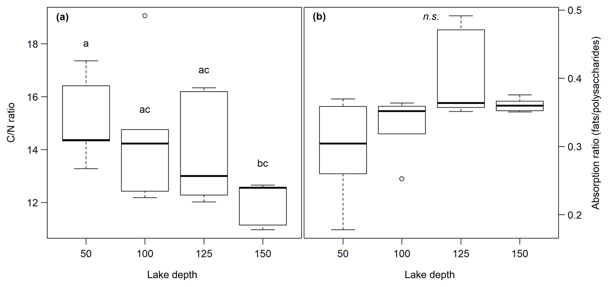
Figure 2(a) C∕N ratio and (b) absorption ratio of fats and polysaccharides at different lake depth categories. Identical lowercase letters indicate C∕N ratios that were not significantly different (i.e., p>0.05) from each other. In the figure, n.s. means that absorption ratios did not exhibit significant differences between lake depths. n(50, 100) = 5, n(125,150) = 6.
Table 2C, N, P, S, Mn and Fe contents, C∕N and FTIR peak ratios (peak maximum for polysaccharides) of identified OM compounds, and their minimum and maximum values. n=16–22.

3.1.2 CO2 and CH4 production rates
Overall, production rates decreased from the shore to the center of the lake. Rates for potential CO2 production at 0–5 cm depth ranged from 10.3±0.0 µmol gC−1 d−1 at site 3.125 to 38.5±2.5 µmol gC−1 d−1 at site 2.100. Potential CH4 production was between 7.3±0.1 µmol gC−1 d−1 at site 3.125 and 33.5±7.2 µmol gC−1 d−1 at site 3.50. Production rates at 5–10 cm depth were always lower compared to the upper sediment layer and were between 7.2±0.1 and 14.7±0.4 µmol gC−1 d−1 for CO2 and between 5.4±0.6 and 14.3±0.3 gC−1 d−1 for CH4. Both CO2 and CH4 production rates showed significant differences between sites (Kruskal–Wallis, p<0.001) and were significantly (Dunn's test, p<0.05) higher at the shore (50+100) than in the center of the lake (125+150) (see Figs. 3, S2 and S3).
CO2 and CH4 production rates decreased with time. CO2 production was highest at the beginning, while CH4 production was impeded and highest only after 3 to 8 d of incubation (see Fig. 4, Table 3). The CO2∕CH4 amount ratio constantly decreased during the incubation with a maximum value of 62.1±58.4 at the beginning of the incubation at site 1.125 and minimum values of 1.2±0.0 at the end of the incubation at site 2.50, approaching ratios of 1 as expected under strictly methanogenic conditions (see also Table 3).
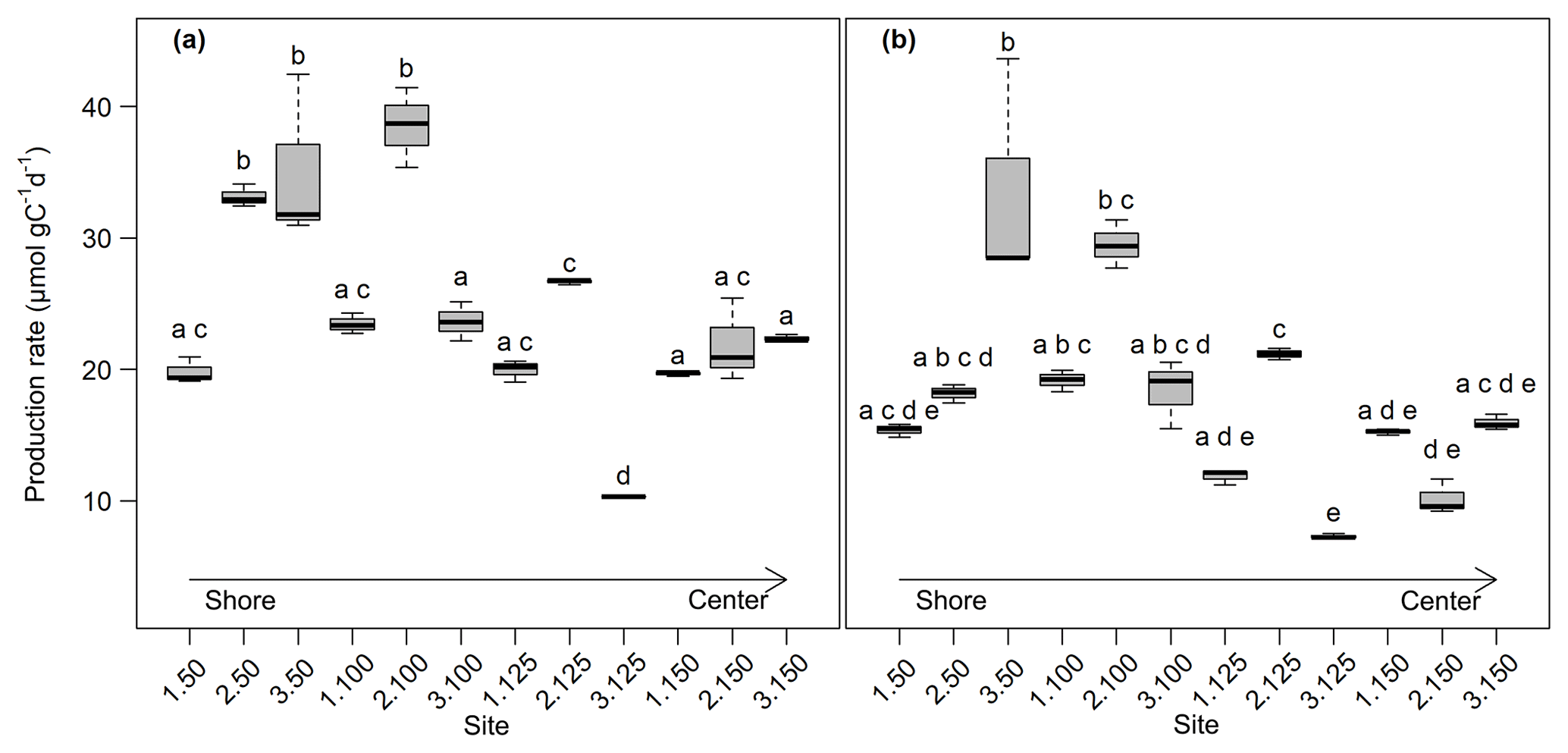
Figure 3CO2 (a) and CH4 (b) production rates at 0–5 cm sediment depth (n=3). Production rates were calculated from the linear regression of concentration increase over time. Bold lines are the median, boxes show the 25 and 75 percentile, and whiskers indicate minima and maxima within 1.5 times the interquartile range. Identical lowercase letters indicate production rates that were not significantly different (i.e., p>0.05) from each other.
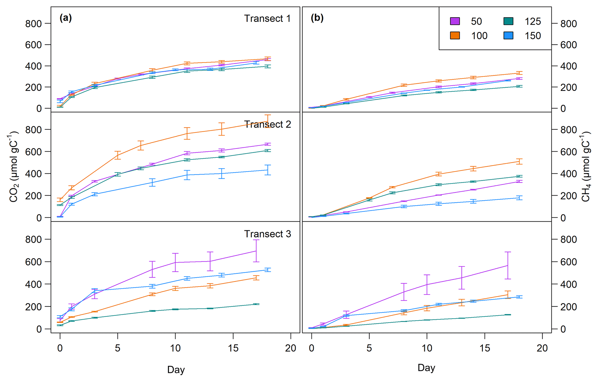
Figure 4CO2 (a) and CH4 (b) production over time at all sites at 0–5 cm sediment depth. Top: transect 1; middle: transect 2; bottom: transect 3. Lines are average values of triplicate measurements (±SD).
Table 3CO2 and CH4 production rates and the CO2 ∕ CH4 amount ratio over time (rates in µmol gC−1 d−1; ratios in µmol). Values in brackets are standard deviations.
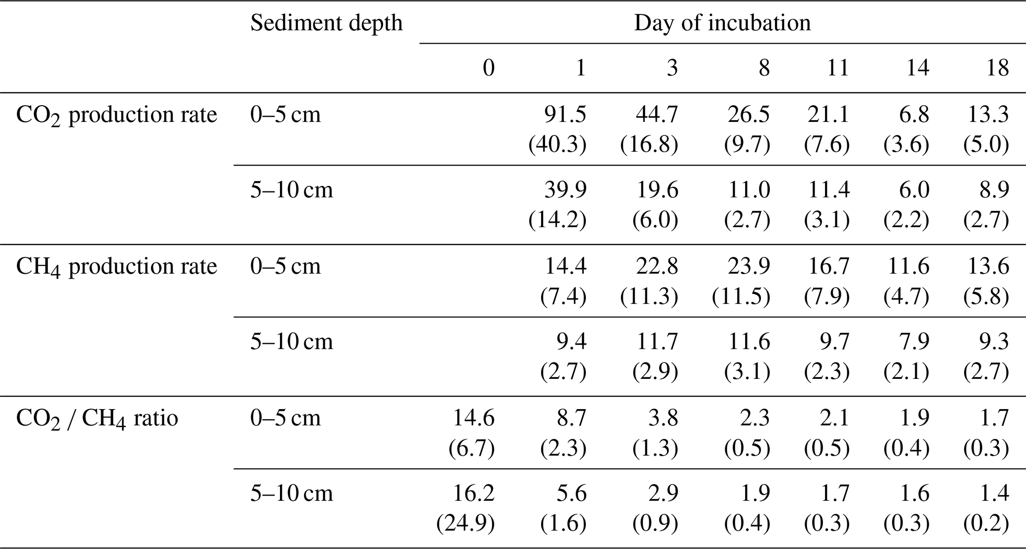
Q10 values were between 1.6±0.1 and 2.2±0.1 for CO2 production rates and between 2.7±0.5 and 11.4±1.0 for CH4 production rates.
Sampling dates did not have any impact on production rates, as confirmed by a Kruskal–Wallis test (CH4: p=0.17; CO2: p=0.76).
Neither CO2 nor CH4 production rates exhibited significant correlations with C content, the C∕N ratio, δ13C or δ15N, but we found significant negative correlations (p<0.01, ρ<−0.6) between all FTIR peak ratios and CO2 and CH4 production rates, as well as of FTIR peak ratios and Q10 values of CH4 production (p<0.05, ) (see Fig. 5; for test statistics, see Table S1 in the Supplement).

Figure 5Correlations between CO2 and CH4 production rates and OM quality parameters as determined by elemental analysis or FTIR spectroscopy. Different colors denote different depth categories (see Fig. 4).
3.1.3 Methanogenic pathways
Both H2 and acetate concentrations increased during the incubation. H2 concentrations were between 0 and 1587.4±170.1 nmol L−1, and acetate concentrations ranged from 219.7±104.3 to 1212.7±11.4 µmol L−1 (see Fig. 6). Gibbs free energy for acetoclastic methanogenesis was between and kJ mol−1, and for hydrogenotrophic methanogenesis it was between and kJ mol−1. Energy yields decreased for the acetoclastic pathway and significantly increased (Mood's median; t0–t6: p<0.05, t3–t6: p<0.001) for the hydrogenotrophic pathway throughout the incubation (see Fig. 6). Energy yields did not differ significantly between lake depths except for the acetoclastic pathway at the end of the incubation (p<0.001) when the energy yield was highest in samples from the center of the lake. Significant differences between all sites were found for the acetoclastic and hydrogenotrophic pathways at the beginning (Kruskal–Wallis, p<0.01) and at the end of the incubation for acetoclastic methanogenesis only (Kruskal–Wallis, p<0.01). H2 concentrations at the end of the experiment exhibited a significant positive correlation with average CO2 (p<0.001, ) and CH4 (p<0.001, ) production rates (for test statistics see Table S2). Further, Gibbs free energy of acetoclastic methanogenesis exhibited a significant positive correlation with the C∕N ratio (p<0.05, ) at the end of the experiment. Acetate concentration at the end of the incubation exhibited significant negative correlations with FTIR peak ratios and the C∕N ratio (p<0.05, ρ<−0.44). Gibbs free energy of hydrogenotrophic methanogenesis exhibited significant positive correlations with FTIR peak ratios of fats, humic acids, phenolics and C content (p<0.05, ρ>0.17); i.e., a high energy yield was associated with low FTIR peak ratios and C content. Correspondingly, H2 concentrations exhibited significant negative correlations with all FTIR peak ratios and C content (p<0.05, ρ<−0.15) (for test statistics see Table S2).

Figure 6(a) Change of Gibbs free energy of hydrogenotrophic (gray) and acetoclastic (white) methanogenesis and of H2 (b) and acetate (c) concentrations over time. More negative ΔGr values correspond to a higher energy yield. Different lowercase letters denote significant differences between sampling dates.
3.1.4 Alternative organic and inorganic EAs
EACOM was between 218.7±97.2 and 545.7±60.3 µmol e− gC−1 at the beginning and decreased on average by 44.9 µmol e− gC−1 until the end of the slurry incubation. The highest values for EACOM were found at site 3.125 corresponding to the lowest measured CH4 production rates at that site. EACinorg was, with values between 2.9±1.0 and 39.2±4.4 µmol e− gC−1, much lower than EACOM and also decreased during the incubation by a mean of 6.4 µmol e− gC−1. EACtot ranged from 250.8±93.9 µmol e− gC−1 at site 3.150 to 551.4±60.3 µmol e− gC−1 at site 3.125 and decreased from the beginning to the end of the incubation by, on average, 51.2 µmol e− gC−1. EDCOM was between 149.5±26.7 and 462.7±18.6 µmol e− gC−1 at the beginning and between 152.9±53.8 and 370.7±196.2 µmol e− gC−1 at the end of the incubation, showing a slight decrease by, on average, 31.4 µmol e− gC−1. The lowest EDCOM at both the beginning and the end of the incubation was found at site 2.100, corresponding to the highest CO2 production rates there (see Fig. 7).
We further found significant differences for EACOM and EACtot (ANOVA, p<0.001) between all sites with the highest average values at site 3.125 and the lowest at sites 1.125 (t0) and 3.150 (t6) (see Fig. S4). Average CO2 and CH4 production rates exhibited a significant negative correlation with initial EDCOM (p<0.05, ), whereas we did not find any significant correlation between the production rates and EAC, electron exchange capacity (EEC; sum of EAC and EDC), or the EAC / EDC ratio, although low CH4 production rates were associated with high EAC. Acetate concentration exhibited significant negative correlations with EACOM and EACtot (p<0.01, <0.001, ρ<−0.38). Gibbs free energy of hydrogenotrophic methanogenesis exhibited significant positive correlations with EACOM and EACtot (p<0.05, ρ=0.43). We did not find any significant correlations between EAC or EDC and OM quality parameters except for EDCOM and the FTIR peak ratio indicative of fats, waxes and lipids (p<0.05, ). Of the inorganic EAs, only total S content in the sediment exhibited a significant negative correlation with CO2 production rates (p<0.05, ) (for test statistics see Table S1).
Calculated potential CO2 production from prevalent organic and inorganic EAs was always lower than the measured CO2 production in slurry incubations and was between 110.5 and 586.4 µmol CO2 eq. gC−1 (see Fig. 8), which could explain 38 % to 91 % of measured CO2 production, whereof 4 % to 51 % were explained by EACOM alone.
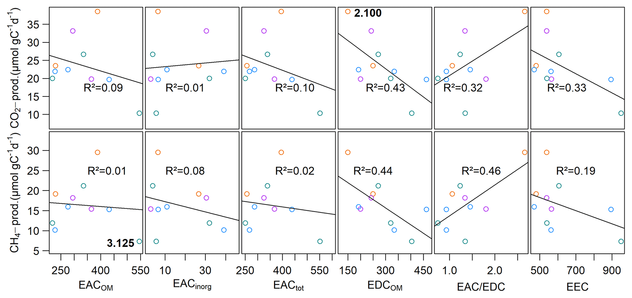
Figure 7Linear regression of CH4 and CO2 production rates with the initial EAC and EDC. Points are mean values of triplicate measurements at each site. At site 2.100, the highest CO2 production rate concurred with lowest EDCOM, and at site 3.125, the lowest CH4 production rate concurred with the highest EACOM. Different colors denote different depth categories (see Fig. 4).

Figure 8Calculated expected CO2 production rate from prevalent EAs vs. measured potential CO2 production rate in slurry incubations. The dashed line shows the closed budget of expected and measured CO2 production.
3.2 Intact sediment core incubations: fluxes, sediment storage change and grain size
CO2 and CH4 fluxes measured from intact sediment core incubations ranged from 10.8±4.4 to 17.9±2.0 and 0.02±0.01 to 1.5±2.6 mmol m−2 d−1, respectively. CH4 ebullition played a major role in cores from sites 2.100 and S.150 and accounted for up to 100 % of the fluxes there. CO2 fluxes at site 3.125 were significantly lower (t-test, p<0.05) than at the other sites, while total CH4 fluxes at site 2.100 were significantly higher (Kruskal–Wallis, p<0.01) compared to all other sites. Fluxes were within the same range as potential production rates in slurry incubations but only partly followed the pattern observed in slurry incubations (see Fig. 9a, b).
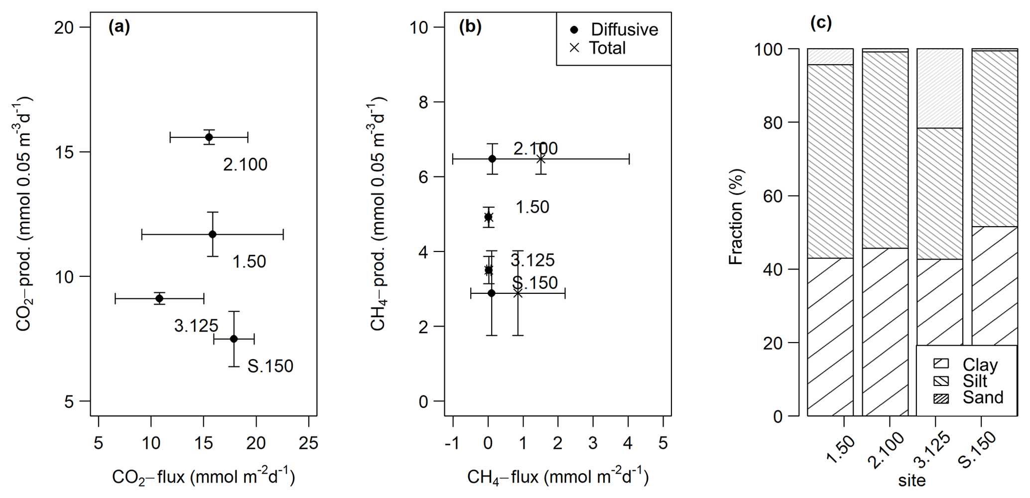
Figure 9Comparison of fluxes obtained from intact sediment core incubations and potential production rates from the slurry incubations (at 0–5 cm sediment depth) for CO2 (a) and diffusive and total CH4 (b). The points are averages – n(slurry incubations) = 3–9, n(CO2 fluxes) = 9–14, n(CH4 fluxes) = 11–13. The horizontal and vertical lines are standard deviations. We decided to display production rates from the 0–5 cm sediment depth as this depth turned out to be the most important for sediment GHG production (see Sects. 3.1.2 and 4.1.1). (c) Relative grain size distribution in intact sediment core incubations.
Table 4Spearman's rank correlation coefficients for CH4 and CO2 fluxes (means of each intact sediment core incubation except for correlations with sediment stock changes for which values from each sampling date were used) and different sediment characteristics; n.s. means that correlations were not significant (p>0.05).

Concentrations of dissolved CH4 and CO2 – Σ(CO2, HCO, CO – in the sediment ranged from 4.0 to 129.5 mmol m−3 (CH4) and from 322.9 to 3811.4 mmol m−3 (CO2), with the lowest values found at site 3.125 and the highest values at S.150. We did not see significant changes in CO2 and CH4 concentrations in the depth profile (see Fig. S5).
Observed changes of CH4 and CO2 concentrations in the sediment of intact cores were overall very low and were between 0.1 and 2.5 mmol d−1 (CH4) and 0.6 and 57.1 mmol d−1 (CO2) in the upper 5 cm of the sediment. These changes were on the same order of magnitude as measured fluxes but did not correlate with them.
Grain sizes distribution differed between the four sites, with site 3.125 having the highest share of sand (21.6 %) and the lowest shares of silt and clay (35.7 % and 42.7 %), whereas the other sites were dominated by finer material and were comprised of less than 5 % of sandy components (see Fig. 9c). CH4 and CO2 fluxes exhibited significant correlations with clay and sand content but not with silt (see Table 4).
Similar to slurry incubations, CH4 fluxes exhibited significant negative correlations with some FTIR peak ratios indicative of recalcitrant OM compounds and with the C∕N ratio but not with C content. CO2 fluxes did not show any significant correlation with OM quality parameters at all (see Table 4).
4.1 Slurry incubations
4.1.1 Variability of CO2 and CH4 production rates and OM quality
Results from the slurry incubation experiment showed that both CO2 and CH4 production rates were – despite its small size - highly variable within the examined lake. CH4 production rates were within the range of previously reported values from lakes in central Sweden, a reservoir in Brazil and in sediments from lakes Stechlin and Geneva in Germany and Switzerland, respectively (Duc et al., 2010; Fuchs et al., 2016; Grasset et al., 2018). CO2 production rates were high compared to rates found in Lake Kinneret in Israel and in the Pantanal and Amazon regions in Brazil, exceeding reported values by a factor of 7 to 100 (Schwarz et al., 2008; Conrad et al., 2011) and supporting the assumption that small lakes generally have higher C turnover rates compared to larger ones.
In all samples, production rates were higher at the beginning of the experiment than toward the end. While CO2 production rates were highest right after the start and then constantly decreased until reaching a plateau around day 8, CH4 production rates peaked after 3 to 8 d and then slowly decreased afterwards, approaching a 1 : 1 CO2:CH4 production ratio. This typically observed three-phase pattern (Yao et al., 1999) might be among other things due to thermodynamic constraints, such as end-product accumulation in the sample vials and subsequent inhibition of respiration and methanogenesis (Beer and Blodau, 2007; Blodau et al., 2011; Bonaiuti et al., 2017). The observed delay in notable CH4 production was expected as prevalent alternative EAs (, Fe3+, , humic substances) likely suppressed methanogenic activity (Lovley et al., 1996; Yao et al., 1999; Fenchel et al., 2012).
Both CO2 and CH4 production rates were higher in the topmost sediment layer compared to the 5–10 cm sediment depth, which suggests that the first centimeters of the sediment play a major role in GHG production as a consequence not only of temperature but also of microbial community distribution and changes in OM quality (Falz et al., 1999; Sobek et al., 2009; Wilkinson et al., 2015). This finding corresponded with decreasing C∕N ratios and increasing FTIR peak ratios with sediment depth. While sediment age typically increases with depth, the OM quality and, thus, reactivity usually decreases with sediment depth as recalcitrant compounds are not being completely mineralized but are instead residually enriched, buried and preserved in the sediment (Avnimelech et al., 1984; Burdige, 2007; Sobek et al., 2009).
Similar to den Heyer and Kalff (1998), we found higher production rates in samples close to the lake shore in contrast to lower production rates in the center, which suggests either that the input of OM (quantity) in the sediments is higher at the shore sites or that the OM quality is more labile and, therefore, more easily degradable. As we did not find any correlations between CO2 or CH4 production rates and sediment C content as proposed, for example, by Conrad et al. (2011) and Romeijn et al. (2019), we instead suggest that the OM quality rather than quantity might be the determining factor for CO2 and CH4 production.
C∕N ratios are frequently used to characterize the degradation state of OM, but we did not find correlations between C∕N ratios and CO2 and CH4 production rates in the slurry incubations. Although OM of autochthonous origin was found to fuel higher degradation rates than allochthonous OM (West et al., 2012; Grasset et al., 2018), we found evidence of predominant inputs of allochthonous (terrestrial) material at sites with higher production rates close to the shore (higher C∕N ratios), whereas sites with lower production rates in the lake center received mainly autochthonous (aquatic) OM, as indicated by lower C∕N ratios (Meyers, 1994). On the other hand, high C∕N ratios also indicate a lower degradation state and, therefore, higher degradation potential, whereas low C∕N ratios are usually typical of highly decomposed OM having a lower CO2 and CH4 production potential (Malmer and Holm, 1984; Kuhry and Vitt, 1996). These two possibilities of interpreting C∕N ratios might be the reason for apparently contradictory findings and the missing relationship between C∕N ratios and CO2 and CH4 production rates.
The abundance of recalcitrant OM compounds (lignin, aromatics, humics, phenols and lipids), as indicated by FTIR peak ratios, proved to be a more suitable explanation for observed CO2 and CH4 production patterns, as indicated by strong significant negative relationships between peak ratios and production rates. All FTIR peak ratios indicative of more refractory components increased toward the lake center, which indicated an increasing predominance of more recalcitrant OM with greater distance from the lake shore and corresponded with decreasing production rates from lake shore to center. At first sight, this was unexpected as allochthonous material is known to be richer in recalcitrant compounds like lignin or aromatics compared to autochthonous biomass and, therefore, is effectively buried in lake sediments (Sobek et al., 2009). However, before reaching the sediment, the internally produced material in the lake center must pass through a deeper water column while undergoing degradation processes such that more decomposed OM reaches the sediment (Meyers, 1994; Torres et al., 2011). As this process might not be of the same importance in shallow lakes compared to deeper lakes, we additionally suggest that the more decomposed OM in the lake center might have undergone degradation processes during resuspension and focusing of small particles as a result of wind-induced bed shearing (Mackay et al., 2011). The less decomposed OM close to the shore might further originate from labile aquatic plant substrates growing at the shoreline (Wetzel, 1992; Cole et al., 2007).
To summarize, the OM degradability does not necessarily depend on its origin, and the OM of terrestrial origin is not necessarily more recalcitrant to degradation by aquatic microorganisms in this study. Sites closer to the shore probably received higher rates of terrestrial OM matter that was less decomposed, whereas autochthonous production in the lake center was overall low due to the low nutrient status of the lake and was already undergoing degradation during sedimentation; this likely led to more recalcitrant OM in the sediment. Earlier studies by West et al. (2012) and Grasset et al. (2018) that found allochthonous material to be less decomposable compared to autochthonous matter were conducted in larger lakes where the influence of the watershed was overall much lower than in our case because larger lakes have a lower perimeter to volume ratio. We hypothesize that in small and nutrient-poor lakes, the pattern might be reversed as the system adapts to overall low productivity and a simultaneously high input of terrestrially produced OM.
In accordance with previous studies (den Heyer and Kalff, 1998; Sobek et al., 2009; Gudasz et al., 2015), we found that with a temperature increase of 10 ∘C, production rates of CO2 doubled, and those of CH4 were even 2 to 11 times higher. Q10 values for CO2 were within the range of earlier reported values by Liikanen et al. (2002) and Bergström et al. (2010), whereas Q10 values for CH4 production were slightly higher than values found by Duc et al. (2010). The large observed range of Q10 values, especially for CH4, implies that responses to temperature increases might not be homogeneously distributed within a lake. The observed negative correlation between Q10 values and FTIR peak ratios further suggests that sites with more labile OM are more susceptive to increasing temperatures in terms of CH4 production, whereas at sites with more recalcitrant OM, the inherent quality of this recalcitrant OM may limit the degradation processes. We, therefore, assume that sediment GHG production – particularly CH4 production – in small and shallow lakes might in the course of global warming increase to a larger extent than in deeper lakes with respect to the fact that shallow waters, as opposed to deeper lakes, do not develop a stable stratification in summer, and thus shallow sediments warm much faster (Jankowski et al., 2006).
The high measured variability in production rates proves (1) that it is necessary to sample lake sediments from different locations in one lake in order to obtain potentials of CO2 and CH4 production representative of the whole lake and (2) that upscaling production rates based on single point measurements may be highly biased. Considering only sediment production rates and based on findings from other studies, it seems that the observed spatial variability of CO2 and CH4 emissions from lakes might to a large extent be controlled by variability in sediment GHG production (Schilder et al., 2013; Bastviken et al., 2015; Natchimuthu et al., 2016; Natchimuthu et al., 2017; Spafford and Risk, 2018). Yet still, as sediment production and emission patterns have so far only been considered separately, other factors driving actual emissions might have been neglected. Therefore, in Sect. 4.2, we further discuss the relationships between CO2 and CH4 production and actual emissions, as assessed in the intact sediment core incubation, and relate them to respective sediment properties.
4.1.2 Methanogenic pathways
To make methanogenesis a profitable reaction for microorganisms, theoretical thresholds of −10.6 kJ mol−1 for the hydrogenotrophic pathway and −12.8 kJ mol−1 for the acetoclastic pathway must be exceeded (Hoehler et al., 2001). Except for a few samples at the beginning of the incubation for the hydrogenotrophic pathway, the theoretical thresholds were always exceeded, suggesting that both pathways could potentially contribute to CH4 production during the whole experiment. Still, this approach does not allow us to evaluate which of the pathways is actually dominant.
Against our expectations, Gibbs free energy of acetoclastic methanogenesis at the end of the incubation was significantly lower (i.e., higher energy yield) in the center of the lake, and ΔGr exhibited a significant positive correlation with the C∕N ratio. Considering that we found the most decomposed material (following peak ratios from FTIR analyses and low C∕N ratios) in the lake center and that low C∕N ratios in this case indicate OM of high recalcitrance, whereas the acetoclastic pathway is thought to predominate with high-quality substrates, we would have expected a reverse pattern (Liu et al., 2017; Berberich et al., 2019). Concomitantly, Gibbs free energy of hydrogenotrophic methanogenesis exhibited significant positive correlations with some FTIR peak ratios indicative of higher contributions of recalcitrant OM compounds, although we expected that a high abundance of recalcitrant OM compounds would make hydrogenotrophic methanogenesis more feasible (Liu et al., 2017). Acetate and H2 concentrations, on the other hand, both exhibited significant negative correlations with some FTIR peak ratios. While this seemed reasonable for acetate concentrations (less acetate available in strongly decomposed OM), this result again proved to be against our expectations in terms of H2 concentrations. This suggests that more recalcitrant material in general slows fermentative processes, delivering both acetate and H2, as a rate-determining step, and all fermentation products are thus kept at low levels.
4.1.3 Alternative EAs
The average EACOM measured in our experiment (302.8±124.6 µmol e− gC−1) was slightly lower but on the same order of magnitude compared to values found by Lau et al. (2015) and Gao et al. (2019) in other lake sediments or peat soils, respectively. Given that C contents in the study by Gao et al. (2019) were much higher than in our study (46.2 %–49.4 %; Agethen and Knorr, 2018) and that Lau et al. (2015) fully oxidized their samples prior to analyses (C content 11.0 %–27.4 %), our measured capacities seem reasonable.
We found that both organic and inorganic EAs decreased during the experiment, indicating that all EAs become similarly depleted with time as they are being reduced by microorganisms. Nevertheless, both absolute EACOM and EACinorg values and relative changes were rather low, which might have been caused by the 1-week preincubation, during which a majority of the reducible organic and inorganic compounds might have already been depleted. Klüpfel et al. (2014) showed that the EAC of oxidized humic acids already strongly declined after 1 d of anoxic incubation and did not change much afterwards. Inorganic EAs were also shown to decrease exponentially during anoxic incubation (Yao et al., 1999). The high CO2 production rates (91.5 µmol gC−1 d−1) at the beginning of the slurry incubation are an indication of these processes.
Sites with higher EACtot had lower CH4 production rates and vice versa as an increased concentration of oxidized humic substances would suppress methanogenic activity on longer timescales, supporting the findings of Agethen et al. (2018) and Gao et al. (2019). Although the relationship between EAC and CH4 production was not significant – probably due to the low number of samples and the sensitivity of the measuring method – a trend was observable.
Non-methanogenic CO2 production could by 38 % to 91 % be explained by prevalent organic and inorganic EAs, whereas organic EAs alone were able to explain up to 52 % of measured CO2 production in slurry incubations. Similar contributions were observed in previous studies from freshwater systems and peatlands, where up to 70 % and 95 % of non-methanogenic CO2 production was explained by total EAC and 25 % to 55 % by decreases in EACOM alone (Lau et al., 2015; Agethen et al., 2018; Gao et al., 2019). The authors suggest several possible reasons for the gap between calculated and experimentally measured CO2 production. Fermentation processes could explain excess CO2, but in this case reduced equivalents of fermentation products such as H2 would be expected to accumulate. Moreover, decarboxylation processes that occur in oxygen-rich, labile OM might occur. Further, the assumption of a nominal oxidation state of C of zero – as assumed in our approach – might be wrong so that when assuming a higher oxidation state, measured changes in EACOM might explain a higher share of CO2 production (Gao et al., 2019). As we did not observe the accumulation of fermentation products and as the sediment under study was not strongly oxidized, we assume these processes are of minor importance and instead suggest that the proportion of unexplained CO2 production can be explained by unknown consumed inorganic EAs during the slurry incubation. In this case, this was most likely solid-phase iron which we found to comprise 2 %–3 % (–137 mg Fe gC−1) of our samples, but we were not able to draw conclusions about its speciation. We suppose this concentration is high enough to reach a closed budget of measured CO2 production and calculated EA turnover; if, on average, 7.8 % (4 %–18.7 %) of solid-phase iron were present as ferric iron, this would suffice to close the CO2 budget.
The large range (4 % to 52 %) of the contribution of organic EAs to CO2 production shows that a distinct small-scale in-lake variability of terminal electron-accepting processes and their contribution to CO2 formation exists in the sediment of Lake Windsborn. Interestingly, the contribution of EACOM was highest at site 3.125 where we observed the lowest CO2 production rates and highest OM recalcitrance. Given that both the absolute C content in the incubation vials and the C:Fe ratio were highest at this site, this supports the findings of Lau et al. (2015), who stated that the contributions of EECOM to total EEC increase with the OC:Fe ratio, indicating more peat-like material.
4.2 Comparison of production rates, fluxes and sediment parameters
Comparing the order of magnitude of potential production rates from slurry incubations and fluxes from intact sediment cores, the results were in good accordance with each other. While CO2 production rates were overall somewhat below measured fluxes, CH4 production rates were considerably higher than actual CH4 fluxes. The differences in CO2 production rates and fluxes can be explained by the influence of the water column; CO2 is produced not only in the sediment but also in the water column, for example, by the degradation of OM or zooplankton respiration (Kling et al., 1992) and can, therefore, contribute to water–atmosphere fluxes. The differences concerning CH4 could be explained by several factors. First, preparing slurry incubations leads to the homogenization of the sediment and higher surface area and, therefore, an even distribution of substrates and microorganisms such that the substrates are more readily available to the microorganisms (Hoehler et al., 2001). Second, sediment fluxes from intact sediment cores may be low compared to homogenized slurry incubations as maximum sediment concentrations were already reached there in shallow depths, suggesting that strong changes in sediment gas concentrations that drive fluxes are likely to occur only in the upper millimeters to centimeters. Additionally, the preparation of slurries reduces the thermodynamic constraints that usually exist in intact profiles due to end-product accumulation (Blodau et al., 2011; Bonaiuti et al., 2017). Third, not all CH4 produced in and emitted by the sediment will reach the water–atmosphere interface because some of the CH4 will be consumed in the oxygenated water column on the way to the surface; through its oxidation in the water column, the amount of CH4 emitted from lakes to the atmosphere can be substantially reduced by 51 % to 100 % (Bastviken et al., 2002, 2008).
Interestingly, spatial patterns of CO2 and CH4 emissions could not be well reproduced from slurry incubations. Although the highest CO2 emissions were observed at site S.150, we found the lowest CO2 production rates there. Additionally, we did not see any correlations between sediment OM quality and CO2 fluxes, suggesting that CO2 production processes in the water column overlying the sediment play a much more important role than in the sediment itself. Moreover, CH4 production rates at sites 1.50 and 3.125 differed significantly from each other, while this was not the case when comparing fluxes. We assume that the different patterns of CH4 fluxes and production can be explained by grain size distribution and, thus, physical sediment properties. Sediment grain size determines sediment pore size, which is essential for the evolution of CH4 bubbles in the sediment (Boudreau et al., 2005). Ebullition is the major component of CH4 fluxes in shallow waters as it can efficiently bypass oxidation in the water column (Bastviken et al., 2004; Wik et al., 2013; Natchimuthu et al., 2016). We found that ebullition was responsible for most of the CH4 fluxes in two of our four intact sediment core incubations, whereas sites with higher shares of sand exhibited less ebullitive fluxes, confirming the findings of Liu et al. (2016, 2018). The authors justify their findings with the dominant pathway of bubble formation in the sediment, which is by displacing surrounding sediment particles. As this mechanism is more efficient in soft silty sediments compared to sandy material, CH4 bubbles likely accumulate more easily in silt, creating a network of macropores and, therefore, conduits for subsequent bubble release. We further found that OM quality partly exhibited significant negative correlations with actual CH4 fluxes but to a lesser extent than with sediment CH4 production. As discussed, when preparing slurry incubations, the physical sediment structure is destroyed so that OM quality likely becomes the major controlling factor for GHG production. These findings suggest that besides OM quality, grain size distribution is a main driver of spatial CH4 flux patterns in intact sediment core incubations and that only a combination of the sediment's physical characteristics and its OM quality could sufficiently explain CH4 emission patterns of lakes.
The missing link between sediment gas storage and both diffusive and ebullitive emissions can potentially be explained by our sampling procedure. While fluxes were partly dominated by bubbles, these bubbles cannot be captured in the sediment by silicon samplers. Silicon samplers rely on the slow diffusion of gas between the pore gas and the sampler, whereas bubbles may form on shorter timescales and can quickly be released to the water column. Thus, concentrations in the bulk sediment stay consistent, while the released bubbles cause high fluxes. Moreover, the resolution of our gas samplers was probably not high enough as they could not cover the uppermost centimeters of the sediment, which we assume to be crucial for diffusive fluxes.
Our results show that there exists a significant spatial variability of CO2 and CH4 production in the sediment of a small and shallow lake and, therefore, that it is not possible to upscale sediment production rates from single point measurements. We further proved that CH4 production strongly depends on temperature and that the extent of temperature dependence might differ within a lake, especially between littoral and central parts due to differences in OM quality. Small lakes seem to be very sensitive to temperature increases in terms of accelerated C cycling, which implies they might become larger sources of CO2 and particularly of CH4 emissions under climate change scenarios. Although such lakes might not react homogeneously, we would expect that sediments in shallower parts might react more sensitively due to shallow water depths and the input of reactive allochthonous OM, which is particularly important for oligotrophic lakes without significant contributions of autochthonous primary production. The strong negative correlations we found between recalcitrant OM compounds and CO2 and CH4 production rates provide evidence that OM quality plays a major role in controlling the mineralization of anoxic lake sediment and can be used to explain and predict patterns of production rates within lakes. Both hydrogenotrophic and acetoclastic methanogenesis were feasible during slurry incubations, but we could not clearly attribute observed patterns to OM quality or EEC; therefore, we suggest that fermentation was the rate-determining step of OM mineralization and that the subsequent consumption of acetate and H2 by electron-accepting processes or methanogenesis kept the levels of these fermentation products low, as expected. We did not find clear patterns between EAC and CH4 production, but organic and inorganic EAs could explain up to 91 % of the observed non-methanogenic CO2 production in slurry incubations.
In sum, measured production rates were only partly reflected in CO2 and CH4 flux patterns obtained from intact sediment core incubations. We suppose that this was because the physical sediment structure (e.g., pore size) was destroyed in the slurry incubations, but these parameters are crucial for the evolution of CH4 bubbles in the sediment. We also suppose that this was because in the slurry incubations, thermodynamic and gas transport constraints that exist in intact anoxic sediment profiles were removed. Further, the interpretation of production rates only would neglect the importance of the water column as a sink of sediment generated CH4 through oxidation and a source of CO2 through degradation and respiration processes, which might then cause discrepancies between observed production and flux rates.
So far, direct flux measurements of CO2 and CH4 between water and the atmosphere seem to be the most accurate way to determine the magnitude and variability of emissions from lakes, but still our study contributes substantially to the understanding of controls underlying potential CO2 and CH4 production in lake sediments and sediment-inherent factors determining emission.
The underlying research data of this study can be found in the Supplement.
The supplement related to this article is available online at: https://doi.org/10.5194/bg-17-5057-2020-supplement.
LP, MS, SS, NP and KHK designed the study. NP and SS carried out the experiments and sample analyses with the help of LP and MS. LP performed data analyses and wrote the paper with the help of NP, SS, KHK and GB.
The authors declare that they have no conflict of interest.
We thank the technicians of the laboratory of the Institute of Landscape Ecology, Ulrike Berning-Mader, Madeleine Supper, Viktoria Ratachin and Melanie Tappe, for sample measurements. We thank Tanja Broder for ICP-OES and Stephan Glatzel for grain size analyses. We further thank Rebecca Pabst, Christina Hackmann, Fabian Lange, Isabelle Rieke, Friederike Ding, Victoria Tietz and Anja Radermacher for their assistance during laboratory work. We also thank Celeste Brennecka for her improvements on the English language and style of the paper.
This research has been supported by the Deutsche Forschungsgemeinschaft (grant no. BL 563/25-1) and the Open-Access Publication Fund of the University of Münster.
This paper was edited by Aninda Mazumdar and reviewed by two anonymous referees.
Achtnich, C., Bak, F., and Conrad, R.: Competition for electron donors among nitrate reducers, ferric iron reducers, sulfate reducers, and methanogens in anoxic paddy soil, Biol. Fert. Soils, 19, 65–72, https://doi.org/10.1007/BF00336349, 1995.
Aeschbacher, M., Sander, M., and Schwarzenbach, R. P.: Novel electrochemical approach to assess the redox properties of humic substances, Environ. Sci. Technol., 44, 87–93, https://doi.org/10.1021/es902627p, 2010.
Aeschbacher, M., Vergari, D., Schwarzenbach, R. P., and Sander, M.: Electrochemical analysis of proton and electron transfer equilibria of the reducible moieties in humic acids, Environ. Sci. Technol., 45, 8385–8394, https://doi.org/10.1021/es201981g, 2011.
Agethen, S. and Knorr, K.-H.: Juncus effusus mono-stands in restored cutover peat bogs – Analysis of litter quality, controls of anaerobic decomposition, and the risk of secondary carbon loss, Soil Biol. Biochem., 117, 139–152, https://doi.org/10.1016/j.soilbio.2017.11.020, 2018.
Agethen, S., Sander, M., Waldemer, C., and Knorr, K.-H.: Plant rhizosphere oxidation reduces methane production and emission in rewetted peatlands, Soil Biol. Biochem., 125, 125–135, https://doi.org/10.1016/j.soilbio.2018.07.006, 2018.
Artz, R. R. E., Chapman, S. J., Jean Robertson, A. H., Potts, J. M., Laggoun-Défarge, F., Gogo, S., Comont, L., Disnar, J.-R., and Francez, A.-J.: FTIR spectroscopy can be used as a screening tool for organic matter quality in regenerating cutover peatlands, Soil Biol. Biochem., 40, 515–527, https://doi.org/10.1016/j.soilbio.2007.09.019, 2008.
Avnimelech, Y., McHenry, J. R., and Ross, J. D.: Decomposition of organic matter in lake sediments, Environ. Sci. Technol., 18, 5–11, https://doi.org/10.1021/es00119a004, 1984.
Bastviken, D., Ejlertsson, J., and Tranvik, L.: Measurement of methane oxidation in lakes: a comparison of methods, Environ. Sci. Technol., 36, 3354–3361, https://doi.org/10.1021/es010311p, 2002.
Bastviken, D., Cole, J., Pace, M., and Tranvik, L.: Methane emissions from lakes: dependence of lake characteristics, two regional assessments, and a global estimate, Global Biogeochem. Cy., 18, GB4009, https://doi.org/10.1029/2004GB002238, 2004.
Bastviken, D., Cole, J. J., Pace, M. L., and van de Bogert, M. C.: Fates of methane from different lake habitats: connecting whole-lake budgets and CH 4 emissions, J. Geophys. Res.-Biogeo., 113, G02024, https://doi.org/10.1029/2007JG000608, 2008.
Bastviken, D., Tranvik, L. J., Downing, J. A., Crill, P. M., and Enrich-Prast, A.: Freshwater methane emissions offset the continental carbon sink, Science (New York, N.Y.), 331, 50 pp., https://doi.org/10.1126/science.1196808, 2011.
Bastviken, D., Sundgren, I., Natchimuthu, S., Reyier, H., and Gålfalk, M.: Technical Note: Cost-efficient approaches to measure carbon dioxide (CO2) fluxes and concentrations in terrestrial and aquatic environments using mini loggers, Biogeosciences, 12, 3849–3859, https://doi.org/10.5194/bg-12-3849-2015, 2015.
Battin, T. J., Luyssaert, S., Kaplan, L. A., Aufdenkampe, A. K., Richter, A., and Tranvik, L. J.: The boundless carbon cycle, Nat. Geosci., 2, 598–600, https://doi.org/10.1038/ngeo618, 2009.
Beer, J. and Blodau, C.: Transport and thermodynamics constrain belowground carbon turnover in a northern peatland, Geochim. Cosmochim. Ac., 71, 2989–3002, https://doi.org/10.1016/j.gca.2007.03.010, 2007.
Berberich, M., Beaulieu, J. J., Hamilton, T. L., Waldo, S., and Buffam, I.: Spatial variability of sediment methane production and methanogen communities within a eutrophic reservoir: importance of organic matter source and quantity, Limnol. Oceanogr., 65, 1336–1358, https://doi.org/10.1002/lno.11392, 2019.
Bergström, I., Kortelainen, P., Sarvala, J., and Salonen, K.: Effects of temperature and sediment properties on benthic CO2 production in an oligotrophic boreal lake, Freshwater Biol., 55, 1747–1757, https://doi.org/10.1111/j.1365-2427.2010.02408.x, 2010.
Biester, H., Knorr, K.-H., Schellekens, J., Basler, A., and Hermanns, Y.-M.: Comparison of different methods to determine the degree of peat decomposition in peat bogs, Biogeosciences, 11, 2691–2707, https://doi.org/10.5194/bg-11-2691-2014, 2014.
Blodau, C.: Thermodynamic control on terminal electron transfer and methanogenesis, in: Aquatic Redox Chemistry, edited by: Tratnyek, P. G., Grundl, T. J., and Haderlein, S. B., American Chemical Society, Washington, DC, 65–83, https://doi.org/10.1021/bk-2011-1071.ch004, 2011.
Blodau, C., Siems, M., and Beer, J.: Experimental burial inhibits methanogenesis and anaerobic decomposition in water-saturated peats, Environ. Sci. Technol., 45, 9984–9989, https://doi.org/10.1021/es201777u, 2011.
Bonaiuti, S., Blodau, C., and Knorr, K.-H.: Transport, anoxia and end-product accumulation control carbon dioxide and methane production and release in peat soils, Biogeochemistry, 133, 219–239, https://doi.org/10.1007/s10533-017-0328-7, 2017.
Boudreau, B. P., Algar, C., Johnson, B. D., Croudace, I., Reed, A., Furukawa, Y., Dorgan, K. M., Jumars, P. A., Grader, A. S., and Gardiner, B. S.: Bubble growth and rise in soft sediments, Geology, 33, 517–520, https://doi.org/10.1130/G21259.1, 2005.
Broder, T., Blodau, C., Biester, H., and Knorr, K. H.: Peat decomposition records in three pristine ombrotrophic bogs in southern Patagonia, Biogeosciences, 9, 1479–1491, https://doi.org/10.5194/bg-9-1479-2012, 2012.
Burdige, D. J.: Preservation of organic matter in marine sediments: controls, mechanisms, and an imbalance in sediment organic carbon budgets?, Chem. Rev., 107, 467–485, https://doi.org/10.1021/cr050347q, 2007.
Cocozza, C., D'Orazio, V., Miano, T. M., and Shotyk, W.: Characterization of solid and aqueous phases of a peat bog profile using molecular fluorescence spectroscopy, ESR and FT-IR, and comparison with physical properties, Org. Geochem., 34, 49–60, https://doi.org/10.1016/S0146-6380(02)00208-5, 2003.
Cole, J. J., Prairie, Y. T., Caraco, N. F., McDowell, W. H., Tranvik, L. J., Striegl, R. G., Duarte, C. M., Kortelainen, P., Downing, J. A., Middelburg, J. J., and Melack, J.: Plumbing the global carbon cycle: integrating inland waters into the terrestrial carbon budget, Ecosystems, 10, 172–185, https://doi.org/10.1007/s10021-006-9013-8, 2007.
Conrad, R.: Contribution of hydrogen to methane production and control of hydrogen concentrations in methanogenic soils and sediments, FEMS Microbiol. Ecol., 28, 193–202, https://doi.org/10.1016/S0168-6496(98)00086-5, 1999.
Conrad, R., Noll, M., Claus, P., Klose, M., Bastos, W. R., and Enrich-Prast, A.: Stable carbon isotope discrimination and microbiology of methane formation in tropical anoxic lake sediments, Biogeosciences, 8, 795–814, https://doi.org/10.5194/bg-8-795-2011, 2011.
den Heyer, C. and Kalff, J.: Organic matter mineralization rates in sediments: a within- and among-lake study, Limnol. Oceanogr., 43, 695–705, https://doi.org/10.4319/lo.1998.43.4.0695, 1998.
Deutscher Wetterdienst (DWD): Observations Germany – Climate – Multi-annual mean 1981–2010, https://opendata.dwd.de/climate_environment/CDC/observations_germany/climate/multi_annual/mean_81-10/, last access: 12 October 2020, 2020.
Dinno, A.: dunn.test version 1.3.5: Dunn's test of multiple comparisons using rank sums, available at: https://CRAN.R-project.org/package=dunn.test (last access: 12 October 2020), 2017.
Downing, J. A.: Emerging global role of small lakes and ponds: little things mean a lot, Limnetica, 29, 9–23, https://doi.org/10.23818/limn.29.02, 2010.
Downing, J. A., Prairie, Y. T., Cole, J. J., Duarte, C. M., Tranvik, L. J., Striegl, R. G., McDowell, W. H., Kortelainen, P., Caraco, N. F., Melack, J. M., and Middelburg, J. J.: The global abundance and size distribution of lakes, ponds, and impoundments, Limnol. Oceanogr., 51, 2388–2397, https://doi.org/10.4319/lo.2006.51.5.2388, 2006.
Duc, N. T., Crill, P., and Bastviken, D.: Implications of temperature and sediment characteristics on methane formation and oxidation in lake sediments, Biogeochemistry, 100, 185–196, https://doi.org/10.1007/s10533-010-9415-8, 2010.
Ellenberg, H., Weber, H. E., Düll, R., Wirth, V., and Werner, W.: Zeigerwerte von Pflanzen in Mitteleuropa, 3rd edn., durchgesehene Auflage, Scripta geobotanica, Volume 18, Verlag Erich Goltze GmbH & Co KG, Göttingen, Germany, 262 pp., 2001.
Falz, K. Z., Holliger, C., Großkopf, R., Liesack, W., Nozhevnikova, A. N., Müller, B., Wehrli, B., and Hahn, D.: Vertical distribution of methanogens in the anoxic sediment of Rotsee (Switzerland), Appl. Environ. Microb., 65, 2402–2408, https://doi.org/10.1128/AEM.65.6.2402-2408.1999, 1999.
Fenchel, T., King, G. M., and Blackburn, T. H.: Bacterial biogeochemistry: The ecophysiology of mineral cycling, 3rd edn., Academic Press/Elsevier, Boston, Mass., 2012.
Fox, J. and Weisberg, S.: An {R} companion to applied regression, Sage, Thousand Oaks, CA, 2011.
Fuchs, A., Lyautey, E., Montuelle, B., and Casper, P.: Effects of increasing temperatures on methane concentrations and methanogenesis during experimental incubation of sediments from oligotrophic and mesotrophic lakes, J. Geophys. Res.-Biogeo., 121, 1394–1406, https://doi.org/10.1002/2016JG003328, 2016.
Gao, C., Sander, M., Agethen, S., and Knorr, K.-H.: Electron accepting capacity of dissolved and particulate organic matter control CO2 and CH4 formation in peat soils, Geochim. Cosmochim. Ac., 245, 266–277, https://doi.org/10.1016/j.gca.2018.11.004, 2019.
Gilboa-Garber, N.: Direct spectrophotometric determination of inorganic sulfide in biological materials and in other complex mixtures, Anal. Biochem., 43, 129–133, https://doi.org/10.1016/0003-2697(71)90116-3, 1971.
Grasset, C., Mendonça, R., Villamor Saucedo, G., Bastviken, D., Roland, F., and Sobek, S.: Large but variable methane production in anoxic freshwater sediment upon addition of allochthonous and autochthonous organic matter, Limnol. Oceanogr., 63, 1488–1501, https://doi.org/10.1002/lno.10786, 2018.
Gudasz, C., Bastviken, D., Steger, K., Premke, K., Sobek, S., and Tranvik, L. J.: Temperature-controlled organic carbon mineralization in lake sediments, Nature, 466, 478–481, https://doi.org/10.1038/nature09186, 2010.
Gudasz, C., Sobek, S., Bastviken, D., Koehler, B., and Tranvik, L. J.: Temperature sensitivity of organic carbon mineralization in contrasting lake sediments, J. Geophys. Res.-Biogeo., 120, 1215–1225, https://doi.org/10.1002/2015JG002928, 2015.
Hoehler, T. M., Alperin, M. J., Albert, D. B., and Martens, C. S.: Apparent minimum free energy requirements for methanogenic Archaea and sulfate-reducing bacteria in an anoxic marine sediment, FEMS Microbiol. Ecol., 38, 33–41, https://doi.org/10.1111/j.1574-6941.2001.tb00879.x, 2001.
Holgerson, M. A. and Raymond, P. A.: Large contribution to inland water CO2 and CH4 emissions from very small ponds, Nat. Geosci., 9, 222–226, https://doi.org/10.1038/NGEO2654, 2016.
Hornibrook, E. R. C., Longstaffe, F. J., and Fyfe, W. S.: Spatial distribution of microbial methane production pathways in temperate zone wetland soils: stable carbon and hydrogen isotope evidence, Geochim. Cosmochim. Ac., 61, 745–753, https://doi.org/10.1016/S0016-7037(96)00368-7, 1997.
Jankowski, T., Livingstone, D. M., Bührer, H., Forster, R., and Niederhauser, P.: Consequences of the 2003 European heat wave for lake temperature profiles, thermal stability, and hypolimnetic oxygen depletion: Implications for a warmer world, Limnol. Oceanogr., 51, 815–819, https://doi.org/10.4319/lo.2006.51.2.0815, 2006.
Kammann, C., Grünhage, L., and Jäger, H.-J.: A new sampling technique to monitor concentrations of CH4, N2O and CO2 in air at well-defined depths in soils with varied water potential, Eur. J. Soil Sci., 52, 297–303, https://doi.org/10.1046/j.1365-2389.2001.00380.x, 2001.
Kampf, J.: Grundwasserlandschaften: Hydrologischer Atlas Rheinland-Pfalz, Landesamt für Umwelt, Wasserwirtschaft und Gewerbeaufsicht Rheinland-Pfalz, Mainz, Landesamt für Umwelt Rheinland-Pfalz, available at: https://lfu.rlp.de/fileadmin/lfu/Wasserwirtschaft/Hydrologischer_Atlas/19_grundwasserlandschaften.pdf (last access: 12 October 2020), 2005.
Kappes, H. and Sinsch, U.: Tolerance of Ceriodaphnia quadrangula and Diaphanosoma brachyurum (Crustacea: Cladocera) to experimental soft water acidification, Hydrobiologia, 534, 109–115, https://doi.org/10.1007/s10750-004-1416-y, 2005.
Kappes, H., Mechenich, C., and Sinsch, U.: Long-term dynamics of Asplanchna priodonta in Lake Windsborn with comments on the diet, Hydrobiologia, 432, 91–100, https://doi.org/10.1023/A:1004022020346, 2000.
Kling, G. W., Kipphut, G. W., and Miller, M. C.: The flux of CO2 and CH4 from lakes and rivers in arctic Alaska, Hydrobiologia, 240, 23–36, https://doi.org/10.1007/BF00013449, 1992.
Klüpfel, L., Piepenbrock, A., Kappler, A., and Sander, M.: Humic substances as fully regenerable electron acceptors in recurrently anoxic environments, Nat. Geosci., 7, 195–200, https://doi.org/10.1038/NGEO2084, 2014.
Konhauser, K.: Introduction to geomicrobiology, John Wiley & Sons Ltd, Hoboken, New Jersey, 425 pp., 2009.
Kuhry, P. and Vitt, D. H.: Fossil carbon/nitrogen ratios as a measure of peat decomposition, Ecology, 77, 271–275, https://doi.org/10.2307/2265676, 1996.
Landesamt für Umwelt (LfU): Seenatlas: Windsborn Kratersee, https://geodaten-wasser.rlp-umwelt.de/ (last access 17 July 2019), 2013.
Lau, M. P., Sander, M., Gelbrecht, J., and Hupfer, M.: Solid phases as important electron acceptors in freshwater organic sediments, Biogeochemistry, 123, 49–61, https://doi.org/10.1007/s10533-014-0052-5, 2015.
Lau, M. P., Sander, M., Gelbrecht, J., and Hupfer, M.: Spatiotemporal redox dynamics in a freshwater lake sediment under alternating oxygen availabilities: combined analyses of dissolved and particulate electron acceptors, Environ. Chem., 13, 826–837, https://doi.org/10.1071/EN15217, 2016.
Li, Y., Zhang, H., Tu, C., Fu, C., Xue, Y., and Luo, Y.: Sources and fate of organic carbon and nitrogen from land to ocean: identified by coupling stable isotopes with C∕N ratio, Estuar. Coast. Shelf S., 181, 114–122, https://doi.org/10.1016/j.ecss.2016.08.024, 2016.
Liikanen, A., Murtoniemi, T., Tanskanen, H., Väisänen, T., and Martikainen, P. J.: Effects of temperature and oxygen availability on greenhouse gas and nutrient dynamics in sediment of a eutrophic and mid-boreal lake, Biogeochemistry, 59, 269–286, https://doi.org/10.1023/A:1016015526712, 2002.
Liu, L., Wilkinson, J., Koca, K., Buchmann, C., and Lorke, A.: The role of sediment structure in gas bubble storage and release, J. Geophys. Res.-Biogeo., 121, 1992–2005, https://doi.org/10.1002/2016JG003456, 2016.
Liu, Y., Conrad, R., Yao, T., Gleixner, G., and Claus, P.: Change of methane production pathway with sediment depth in a lake on the Tibetan plateau, Palaeogeogr. Palaeocl., 474, 279–286, https://doi.org/10.1016/j.palaeo.2016.06.021, 2017.
Liu, L., de Kock, T., Wilkinson, J., Cnudde, V., Xiao, S., Buchmann, C., Uteau, D., Peth, S., and Lorke, A.: Methane bubble growth and migration in aquatic sediments observed by X-ray μCT, Environ. Sci. Technol., 52, 2007–2015, https://doi.org/10.1021/acs.est.7b06061, 2018.
Lojen, S., Ogrinc, N., and Dolenec, T.: Decomposition of sedimentary organic matter and methane formation in the recent sediment of Lake Bled (Slovenia), Chem. Geol., 159, 223–240, https://doi.org/10.1016/S0009-2541(99)00032-7, 1999.
Lovley, D. R., Coates, J. D., Blunt-Harris, E. L., Phillips, E. J. P., and Woodward, J. C.: Humic substances as electron acceptors for microbial respiration, Nature, 382, 445–448, https://doi.org/10.1038/382445a0, 1996.
Mackay, E. B., Jones, I. D., Folkard, A. M., and Barker, P.: Contribution of sediment focussing to heterogeneity of organic carbon and phosphorus burial in small lakes, Freshwater Biol., 57, 290–304, https://doi.org/10.1111/j.1365-2427.2011.02616.x, 2011.
Malmer, N. and Holm, E.: Variation in the C∕N-quotient of peat in relation to decomposition rate and age determination with 210 Pb, Oikos, 43, 171–182, https://doi.org/10.2307/3544766, 1984.
McLatchey, G. P. and Reddy, K. R.: Regulation of organic matter decomposition and nutrient release in a wetland soil, J. Environ. Qual., 27, 1268–1274, https://doi.org/10.2134/jeq1998.00472425002700050036x, 1998.
Megonigal, J. P., Hines, M. E., and Visscher, P. T.: Anaerobic metabolism: linkages to trace gases and aerobic processes, in: Treatise on Geochemistry, edited by: Holland, H. D. and Turekian, K. K., Elsevier, Amsterdam, Boston, Heidelberg, London, New York, Oxford, Paris, San Diego, San Francisco, Singapore, Sydney, Tokyo, 317–424, https://doi.org/10.1016/B0-08-043751-6/08132-9, 2003.
Meyer, W.: Geologie der Eifel, 4th edn., Schweizerbart'sche Verlagsbuchhandlung, Stuttgart, Germany, 2013.
Meyers, P. A.: Preservation of elemental and isotopic source identification of sedimentary organic matter, Chem. Geol., 114, 289–302, https://doi.org/10.1016/0009-2541(94)90059-0, 1994.
Miyajima, T., Wada, E., Hanba, Y. T., and Vijarnsorn, P.: Anaerobic mineralization of indigenous organic matters and methanogenesis in tropical wetland soils, Geochim. Cosmochim. Ac., 61, 3739–3751, https://doi.org/10.1016/S0016-7037(97)00189-0, 1997.
Muri, G. and Wakeham, S. G.: Organic matter and lipids in sediments of Lake Bled (NW Slovenia): Source and effect of anoxic and oxic depositional regimes, Org. Geochem., 37, 1664–1679, https://doi.org/10.1016/j.orggeochem.2006.07.016, 2006.
Natchimuthu, S., Sundgren, I., Gålfalk, M., Klemedtsson, L., Crill, P., Danielsson, Å., and Bastviken, D.: Spatio-temporal variability of lake CH4 fluxes and its influence on annual whole lake emission estimates, Limnol. Oceanogr., 61, S13–S26, https://doi.org/10.1002/lno.10222, 2016.
Natchimuthu, S., Sundgren, I., Gålfalk, M., Klemedtsson, L., and Bastviken, D.: Spatiotemporal variability of lake pCO2 and CO2 fluxes in a hemiboreal catchment, J. Geophys. Res.-Biogeo., 122, 30–49, https://doi.org/10.1002/2016JG003449, 2017.
Niemeyer, J., Chen, Y., and Bollag, J.-M.: Characterization of humic acids, composts, and peat by diffuse reflectance Fourier-Transform infrared spectroscopy, Soil Sci. Soc. Am. J., 56, 135–140, https://doi.org/10.2136/sssaj1992.03615995005600010021x, 1992.
Nordstrom, D. K., and Munoz, J. L.: Geochemical thermodynamics, 2nd edn., Blackwell Scientific, Boston, Mass, 1994.
OENorm B 4412: 1974 07 01, Erd- und Grundbau, Untersuchung von Bodenproben, Korngrößenverteilung, Austrian Standards International, 1974.
OENorm L 1050: 2016 03 15, Boden als Pflanzenstandort – Begriffe und Untersuchungsverfahren, Austrian Standards International, 2016.
OENorm L 1061-2: 2019 03 01, Physikalische Bodenuntersuchungen – Bestimmung der Korngrößenverteilung des Mineralbodens in land- und forstwirtschaftlich genutzten Böden – Teil 2: Feinboden, Austrian Standards International, 2019.
Ostrovsky, I. and Tęgowski, J.: Hydroacoustic analysis of spatial and temporal variability of bottom sediment characteristics in Lake Kinneret in relation to water level fluctuation, Geo.-Mar. Lett., 30, 261–269, https://doi.org/10.1007/s00367-009-0180-4, 2010.
R Core Team: R: A language and environment for statistical computing, R Foundation for Statistical Computing, Vienna, Austria, https://www.R-project.org/, 2018.
Raymond, P. A., Hartmann, J., Lauerwald, R., Sobek, S., McDonald, C., Hoover, M., Butman, D., Striegl, R., Mayorga, E., Humborg, C., Kortelainen, P., Dürr, H., Meybeck, M., Ciais, P., and Guth, P.: Global carbon dioxide emissions from inland waters, Nature, 503, 355–359, https://doi.org/10.1038/nature12760, 2013.
Regnier, P., Friedlingstein, P., Ciais, P., Mackenzie, F. T., Gruber, N., Janssens, I. A., Laruelle, G. G., Lauerwald, R., Luyssaert, S., Andersson, A. J., Arndt, S., Arnosti, C., Borges, A. V., Dale, A. W., Gallego-Sala, A., Goddéris, Y., Goossens, N., Hartmann, J., Heinze, C., Ilyina, T., Joos, F., LaRowe, D. E., Leifeld, J., Meysman, F. J. R., Munhoven, G., Raymond, P. A., Spahni, R., Suntharalingam, P., and Thullner, M.: Anthropogenic perturbation of the carbon fluxes from land to ocean, Nat. Geosci., 6, 597–607, https://doi.org/10.1038/NGEO1830, 2013.
Romeijn, P., Comer-Warner, S. A., Ullah, S., Hannah, D. M., and Krause, S.: Streambed organic matter controls on carbon dioxide and methane emissions from streams, Environ. Sci. Technol., 53, 2364–2374, https://doi.org/10.1021/acs.est.8b04243, 2019.
Sander, R.: Compilation of Henry's law constants (version 4.0) for water as solvent, Atmos. Chem. Phys., 15, 4399–4981, https://doi.org/10.5194/acp-15-4399-2015, 2015.
Schilder, J., Bastviken, D., van Hardenbroek, M., Kankaala, P., Rinta, P., Stötter, T., and Heiri, O.: Spatial heterogeneity and lake morphology affect diffusive greenhouse gas emission estimates of lakes, Geophys. Res. Lett., 40, 5752–5756, https://doi.org/10.1002/2013GL057669, 2013.
Schink, B.: Energetics of syntrophic cooperation in methanogenic degradation, Microbiol. Mol. Biol. R., 61, 262–280, http://nbn-resolving.de/urn:nbn:de:bsz:352-opus-27009, 1997.
Schoell, M.: Multiple origins of methane in the Earth, Chem. Geol., 71, 1–10, https://doi.org/10.1016/0009-2541(88)90101-5, 1988.
Schwarz, J. I. K., Eckert, W., and Conrad, R.: Response of the methanogenic microbial community of a profundal lake sediment (Lake Kinneret, Israel) to algal deposition, Limnol. Oceanogr., 53, 113–121, https://doi.org/10.4319/lo.2008.53.1.0113, 2008.
Seeberg-Elverfeldt, J., Schlüter, M., Feseker, T., and Kölling, M.: Rhizon sampling of porewaters near the sediment-water interface of aquatic systems, Limnol. Oceanogr. Methods, 3, 361–371, https://doi.org/10.4319/lom.2005.3.361, 2005.
Segers, R.: Methane production and methane consumption: a review of processes underlying wetland methane fluxes, Biogeochemistry, 41, 23–51, https://doi.org/10.1023/A:1005929032764, 1998.
Sobek, S., Durisch-Kaiser, E., Zurbrügg, R., Wongfun, N., Wessels, M., Pasche, N., and Wehrli, B.: Organic carbon burial efficiency in lake sediments controlled by oxygen exposure time and sediment source, Limnol. Oceanogr., 54, 2243–2254, https://doi.org/10.4319/lo.2009.54.6.2243, 2009. Spafford, L. and Risk, D.: Spatiotemporal variability in lake-atmosphere net CO2 exchange in the littoral zone of an oligotrophic lake, J. Geophys. Res.-Biogeo., 123, 1260–1276, https://doi.org/10.1002/2017JG004115, 2018.
Stumm, W. and Morgan, J. J.: Aquatic chemistry: Chemical equilibria and rates in natural waters, 3rd edn., John Wiley & Sons Inc, New York, Chichester, Brisbane, Toronto, Singapore, 1995.
Tamura, H., Goto, K., Yotsuyanagi, T., and Nagayama, M.: Spectrophotometric determination of iron(II) with 1,10-phenanthroline in the presence of large amounts of iron(III), Talanta, 21, 314–318, https://doi.org/10.1016/0039-9140(74)80012-3, 1974.
Tfaily, M. M., Cooper, W. T., Kostka, J. E., Chanton, P. R., Schadt, C. W., Hanson, P. J., Iversen, C. M., and Chanton, J. P.: Organic matter transformation in the peat column at Marcell Experimental Forest: Humification and vertical stratification, J. Geophys. Res.-Biogeo., 119, 661–675, https://doi.org/10.1002/2013JG002492, 2014.
Tolu, J., Rydberg, J., Meyer-Jacob, C., Gerber, L., and Bindler, R.: Spatial variability of organic matter molecular composition and elemental geochemistry in surface sediments of a small boreal Swedish lake, Biogeosciences, 14, 1773–1792, https://doi.org/10.5194/bg-14-1773-2017, 2017.
Torres, I. C., Inglett, K. S., and Reddy, K. R.: Heterotrophic microbial activity in lake sediments: effects of organic electron donors, Biogeochemistry, 104, 165–181, https://doi.org/10.1007/s10533-010-9494-6, 2011. Updegraff, K., Pastor, J., Bridgham, S. D., and Johnston, C. A.: Environmental and substrate controls over carbon and nitrogen mineralization in northern wetlands, Ecol. Appl., 5, 151–163, https://doi.org/10.2307/1942060, 1995.
Verpoorter, C., Kutser, T., Seekell, D. A., and Tranvik, L. J.: A global inventory of lakes based on high-resolution satellite imagery, Geophys. Res. Lett., 41, 6396–6402, https://doi.org/10.1002/2014GL060641, 2014.
Walpen, N., Schroth, M. H., and Sander, M.: Quantification of phenolic antioxidant moieties in dissolved organic matter by flow-injection analysis with electrochemical detection, Environ. Sci. Technol., 50, 6423–6432, https://doi.org/10.1021/acs.est.6b01120, 2016.
Walpen, N., Getzinger, G. J., Schroth, M. H., and Sander, M.: Electron-donating phenolic and electron-accepting quinone moieties in peat dissolved organic matter: quantities and redox transformations in the context of peat biogeochemistry, Environ. Sci. Technol., 52, 5236–5245, https://doi.org/10.1021/acs.est.8b00594, 2018.
West, W. E., Coloso, J. J., and Jones, S. E.: Effects of algal and terrestrial carbon on methane production rates and methanogen community structure in a temperate lake sediment, Freshwater Biol., 57, 949–955, https://doi.org/10.1111/j.1365-2427.2012.02755.x, 2012.
Wetzel, R. G.: Gradient-dominated ecosystems: sources and regulatory functions of dissolved organic matter in freshwater ecosystems, in: Dissolved Organic Matter in Lacustrine Ecosystems: Energy Source and System Regulator, edited by: Salonen, K., Kairesalo, T., and Jones, R. I., Springer Netherlands, Dordrecht, 181–198, https://doi.org/10.1007/978-94-011-2474-4_14, 1992.
Whiticar, M. J.: Carbon and hydrogen isotope systematics of bacterial formation and oxidation of methane, Chem. Geol., 161, 291–314, https://doi.org/10.1016/S0009-2541(99)00092-3, 1999. Wik, M., Crill, P. M., Varner, R. K., and Bastviken, D.: Multiyear measurements of ebullitive methane flux from three subarctic lakes, J. Geophys. Res.-Biogeo., 118, 1307–1321, https://doi.org/10.1002/jgrg.20103, 2013.
Wilkinson, J., Maeck, A., Alshboul, Z., and Lorke, A.: Continuous seasonal river ebullition measurements linked to sediment methane formation, Environ. Sci. Technol., 49, 13121–13129, https://doi.org/10.1021/acs.est.5b01525, 2015.
Yao, H., Conrad, R., Wassmann, R., and Neue, H. U.: Effect of soil characteristics on sequential reduction and methane production in sixteen rice paddy soils from China, the Philippines, and Italy, Biogeochemistry, 47, 269–295, https://doi.org/10.1007/BF00992910, 1999.