the Creative Commons Attribution 4.0 License.
the Creative Commons Attribution 4.0 License.
 | 23 Nov 2020
Modelling the habitat preference of two key Sphagnum species in a poor fen as controlled by capitulum water content
Jinnan Gong
Nigel Roulet
Steve Frolking
Heli Peltola
Anna M. Laine
Nicola Kokkonen
Eeva-Stiina Tuittila
Current peatland models generally treat vegetation as static, although plant community structure is known to alter as a response to environmental change. Because the vegetation structure and ecosystem functioning are tightly linked, realistic projections of peatland response to climate change require the inclusion of vegetation dynamics in ecosystem models. In peatlands, Sphagnum mosses are key engineers. Moss community composition primarily follows habitat moisture conditions. The known species habitat preference along the prevailing moisture gradient might not directly serve as a reliable predictor for future species compositions, as water table fluctuation is likely to increase. Hence, modelling the mechanisms that control the habitat preference of Sphagna is a good first step for modelling community dynamics in peatlands. In this study, we developed the Peatland Moss Simulator (PMS), which simulates the community dynamics of the peatland moss layer. PMS is a process-based model that employs a stochastic, individual-based approach for simulating competition within the peatland moss layer based on species differences in functional traits. At the shoot-level, growth and competition were driven by net photosynthesis, which was regulated by hydrological processes via the capitulum water content. The model was tested by predicting the habitat preferences of Sphagnum magellanicum and Sphagnum fallax – two key species representing dry (hummock) and wet (lawn) habitats in a poor fen peatland (Lakkasuo, Finland). PMS successfully captured the habitat preferences of the two Sphagnum species based on observed variations in trait properties. Our model simulation further showed that the validity of PMS depended on the interspecific differences in the capitulum water content being correctly specified. Neglecting the water content differences led to the failure of PMS to predict the habitat preferences of the species in stochastic simulations. Our work highlights the importance of the capitulum water content with respect to the dynamics and carbon functioning of Sphagnum communities in peatland ecosystems. Thus, studies of peatland responses to changing environmental conditions need to include capitulum water processes as a control on moss community dynamics. Our PMS model could be used as an elemental design for the future development of dynamic vegetation models for peatland ecosystems.
- Article
(3813 KB) - Full-text XML
-
Supplement
(2215 KB) - BibTeX
- EndNote


Peatlands have important roles in the global carbon cycle, as they store about 30 % of the world's soil carbon (Gorham, 1991; Hugelius et al., 2013). Environmental changes, such as climate warming and land use changes, are expected to impact the carbon functioning of peatland ecosystems (Tahvanainen, 2011). Predicting the functioning of peatlands under environmental change conditions requires models to quantify the interactions among ecohydrological, ecophysiological, and biogeochemical processes. These processes are known to be strongly regulated by vegetation (Riutta et al., 2007; Wu and Roulet, 2014), which can change over decadal timescales under changing hydrological conditions (Tahvanainen, 2011). Peatland models have generally considered vegetation structure in an unrealistic manner: as a static component (e.g. Frolking et al., 2002; Wania et al., 2009). The recent regional-scale peatland model developed by Chaudhary et al. (2017) includes dynamic vegetation shifts among a single moss plant functional type (PFT) and four vascular PFTs; however, in order to support realistic predictions of peatland functioning and global biogeochemical cycles, the mechanisms that drive changes in moss community structure need to be identified and integrated with ecosystem processes.
A major fraction of peatland biomass is formed by Sphagnum mosses (Hayward and Clymo, 1983; Vitt, 2000). Although individual Sphagnum species often have narrow habitat niches (Johnson et al., 2015), different Sphagnum species replace each other along the water table gradient; therefore, as a genus, Sphagnum species are spread across a wide range of water table conditions (Rydin and McDonald, 1985; Andrus, 1986; Rydin, 1993; Laine et al., 2009). The species composition of the Sphagnum community strongly affects ecosystem processes such as carbon sequestration and peat formation through interspecific variability in species traits including the photosynthetic potential and litter quality (Clymo, 1970; O'Neill, 2000; Vitt, 2000; Turetsky, 2003). The Sphagnum biomass and litter production gradually raises the moss carpet, which feeds back into the species composition (Robroek et al., 2009). Hence, modelling the moss community dynamics is fundamental for predicting temporal changes in peatland vegetation. As the distribution of Sphagnum species primarily follows the variability in the peatland water table (Andrus, 1986; Väliranta et al., 2007), modelling the habitat preference of Sphagnum species along a moisture gradient could be a good first step in predicting moss community dynamics (Blois et al., 2013).
For a given Sphagnum species, the optimal habitat represents the environmental conditions for it to achieve higher rates of net photosynthesis and shoot elongation than its peers (Titus and Wagner, 1984; Rydin and McDonald, 1985; Rydin, 1997; Robroek et al., 2007a; Keuper et al., 2011). The capitulum water content and water storage, which are determined by the balance between the evaporative loss and water gains from capillary rise and precipitation, represent one of the most important controls on net photosynthesis (Titus and Wagner, 1984; Murray et al., 1989; Van Gaalen et al., 2007; Robroek et al., 2009). To quantify the water processes in mosses, hydrological models have been developed to simulate the water movement between the moss carpet and the peat underneath, as regulated by the variations in meteorological conditions and energy balance (Price, 2008; Price and Whittington, 2010). On the other hand, experimental work has addressed the species-specific responses of net photosynthesis to changes in the capitulum water content (Titus and Wagner, 1984; Hájek and Beckett, 2008; Schipperges and Rydin, 1998) and light intensity (Rice et al., 2008; Laine et al., 2011; Bengtsson et al., 2016). Net photosynthesis and hydrological processes are linked via capitulum water retention, which controls the response of the capitulum water content to water potential changes (Jassey and Signarbieux, 2019). However, these mechanisms have not been integrated with ecosystem processes in model simulations.
Along with the capitulum water processes, modelling the habitat preference of Sphagna requires the quantification of the competition among mosses, i.e. the “race for space” (Rydin, 1993, 1997; Robroek et al., 2007a; Keuper et al., 2011): Sphagnum shoots can form new capitula and spread laterally if there is space available. This reduces or eliminates the light source for any plant that is buried by its peers (Robroek et al., 2009). As the competition occurs between neighbouring shoots, its modelling requires downscaling interlinked water–energy processes from the ecosystem to the shoot level. Thus, Sphagnum competition needs to be modelled as spatial processes, considering the fact that spatial coexistence and the variations in functional traits among shoot individuals may impact the community dynamics (Bolker et al., 2003; Amarasekare, 2003). However, coexistence generally relies on simple coefficients to describe the interactions among individuals (e.g. Czárán and Iwasa, 1998; Anderson and Neuhauser, 2000; Gassmann et al., 2003; Boulangeat et al., 2018) and is consequently decoupled from environmental fluctuation or the stochasticity of biophysiological processes.
This study aims to develop and test a model, the Peatland Moss Simulator (PMS), to simulate community dynamics within the peatland moss layer that results in realistic habitat preference of Sphagnum species along a moisture gradient. In PMS, community dynamics is driven by Sphagnum photosynthesis. Photosynthesis, in turn, is regulated by capitulum water retention through the capitulum moisture content. Therefore, we hypothesize that the water retention of the capitula is the mechanism driving moss community dynamics. We test the model validity using data from an experiment based on two Sphagnum species that have different positions along the moisture gradient in the same peatland site. If our hypothesis holds, the model will (1) correctly predict the competitiveness of the two species in wet and dry habitats and (2) fail to predict competitiveness if the capitulum water retention and water content of the two species are not correctly specified.
2.1 Study site
The peatland site being modelled is located in Lakkasuo, Orivesi, Finland (61∘47′ N; 24∘18′ E). The site is a poor fen fed by mineral inflows from a nearby esker (Laine et al., 2004). Most of the site is formed by lawns dominated by Sphagnum recurvum complex (Sphagnum fallax accompanied by Sphagnum flexuosum and Sphagnum angustifolium) and Sphagnum papillosum. Less than 10 % of the surface is occupied by hummocks, inhabited by Sphagnum magellanicum and Sphagnum fuscum, which are 15–25 cm higher than the lawn surfaces. Both microforms are covered by continuous Sphagnum carpet with a sparse vascular plant cover (12 % Carex cover on average), which spread homogeneously over the topography. The annual mean water table was 15.6±5.0 cm deep at the lawn surface (Kokkonen et al., 2019). More information about the site can be found in Kokkonen et al. (2019).
2.2 Model outline
The Peatland Moss Simulator (PMS) is a process-based, stochastic model that simulates the temporal dynamics of a Sphagnum community as driven by variations in precipitation, irradiation, and energy flow with individual-based interactions (Fig. 1). In PMS, the studied ecosystem is seen as a dual-column system consisting of hydrologically connected habitats of hummocks and lawns (community environment in Fig. 1). For each habitat type, the community area is downscaled to two-dimensional cells representing the scale of individual shoots (i.e. 1 cm2). Each grid cell can be occupied by one capitulum from a single Sphagnum species. The community dynamics, i.e. the changes in species abundances, are driven by the growth and competition of Sphagnum shoots at the grid-cell level (Module I in Fig. 1). These processes are regulated by the grid-cell-specific conditions of water and energy (Module II in Fig. 1), which are derived from the community environment (Module III in Fig. 1).
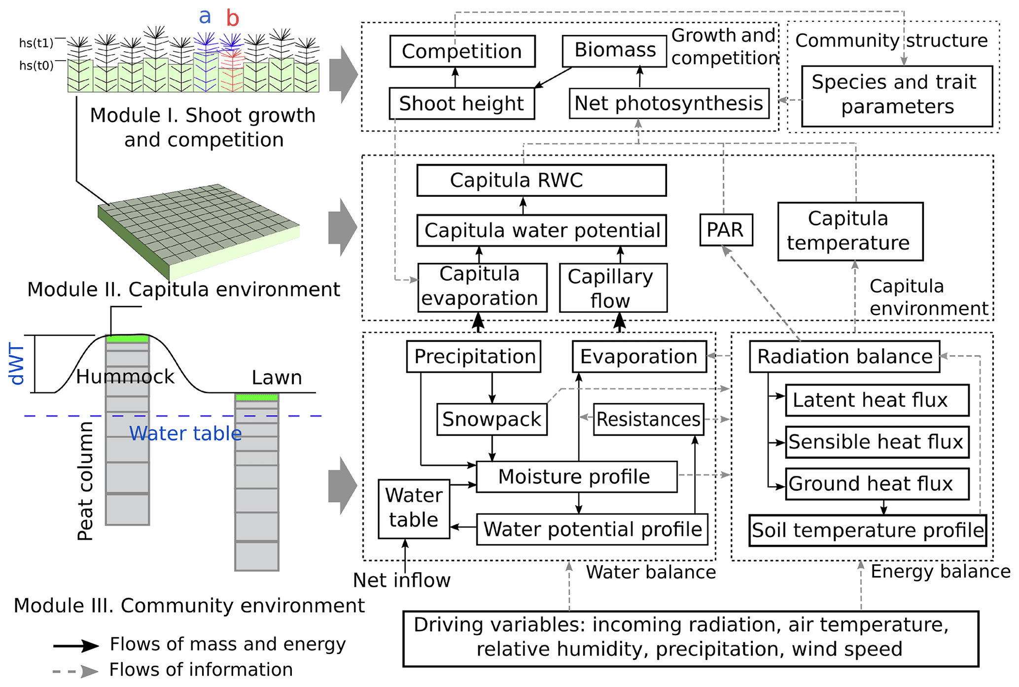
In this study, we focused on developing modules I and II (Sect. 2.3) and employed an available soil–vegetation–atmosphere transport (SVAT) model (Gong et al., 2013, 2016) to describe the water–energy processes for Module III (Appendix A). We assumed that the temporal variation in the water table was similar in lawns and hummocks and that the hummock–lawn differences in the water table (dWT in Fig. 1) followed their difference in surface elevations (Wilson, 2012). At the grid-cell level, the photosynthesis of capitula drove the biomass growth and elongation of shoots, which led to the competition between adjacent grid cells. The net photosynthesis rate was controlled by the capitulum water content, Wcap, which was defined by the capitulum water retention in relation to the water potential, h (Sect. 2.4). The values for functional traits that regulate the growth and competition processes were randomly selected within their normal distribution measured in the field (Sect. 2.4). Unknown parameters that related the lateral water flows of the site are estimated using a machine-learning approach (Sect. 2.5). Finally, a Monte Carlo simulation was used to support the analysis of the habitat preferences of Sphagnum species and hypothesis tests (Sect. 2.6). The list of symbols used is given in Appendix E.
Table 1Species-specific values of morphological and photosynthetic parameters for S. magellanicum and S. fallax. The parameters include the capitulum density (DS), the capitulum biomass (Bcap), the specific height of the stem (Hspc), the maximal gross photosynthesis rate at 20 ∘C (Pm20), the respiration rate at 20 ∘C (Rs20), the half-saturation point of photosynthesis (αPPFD), and the polynomial coefficients (aW0, aW1, and aW2) for the responses of net photosynthesis to capitulum water content. Parameter values are given as the mean ± standard deviation.
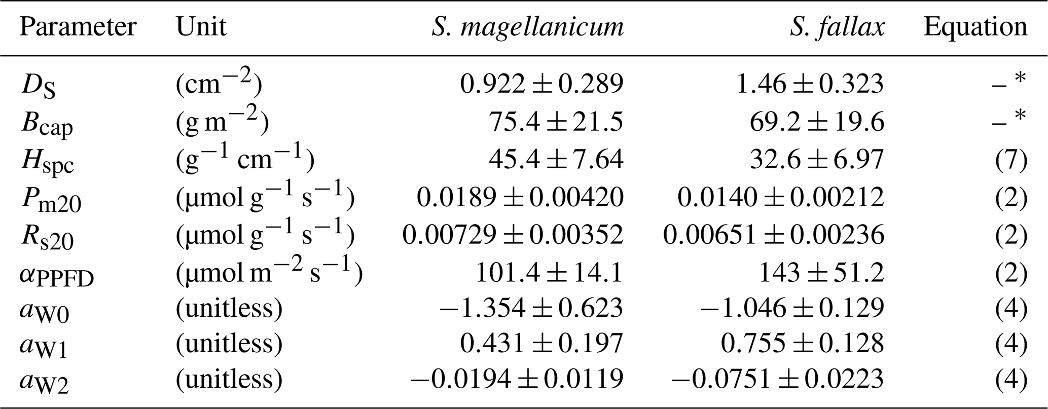
∗ The parameter was used in the linear models predicting the log10-transformed capitulum water potential (h) and the bulk resistance (rbulk) for S. fallax and S. magellanicum. The capitulum density and photosynthetic parameter values measured here are well within the range of those reported in the literature for these species (McCarter and Price, 2014; Laing et al., 2014; Bengtsson et al., 2016; Korrensalo et al., 2016).
2.3 Model development
2.3.1 Calculating shoot growth and competition of Sphagnum mosses (Module I)
Calculation of Sphagnum growth
To model the grid-cell biomass production and height increment, we assumed that capitula were the main parts of the shoots responsible for photosynthesis and the production of new tissues, instead of the stem sections underneath. We employed a hyperbolic light-saturation function (Larcher, 2003) to calculate the net photosynthesis, which was parameterized based on empirical measurements made from the target species collected from the study site (see Appendix B for materials and methods):
where subscript 20 denotes the variable value measured at 20 ∘C; Rs is the mass-based respiration rate (µmol g−1 s−1); Pm is the mass-based rate of maximal gross photosynthesis (µmol g−1 s−1); PPFD is the photosynthetic photon flux density (µmol m−2 s−1); Bcap is the capitulum biomass; and αPPFD is the half-saturation point (µmol m−2 s−1) for photosynthesis.
By adding multipliers for the capitula water content (fW) and temperature (fT) to Eq. (1), the net photosynthesis rate A (µmol m−2 s−1) was calculated as follows:
where fW(Wcap) describes the responses of A to the capitulum water content, Wcap; and fT(T) describes the responses of Pm to the capitulum temperature T (Korrensalo et al., 2017). fW(Wcap) was estimated based on the empirical measurements (see Sect. 2.4 and Appendix B). The temperature response fR(T) is a Q10 function that describes the temperature sensitivity of Rs (Frolking et al., 2002):
where Q10 is the sensitivity coefficient; T is the capitulum temperature (∘C); and Topt (20 ∘C) is the reference temperature of respiration.
The response of A to Wcap (fW(Wcap); Eq. 2) was described as a second-order polynomial function:
where aW0, aW1, and aW2 are coefficients.
Plants can store carbohydrates as nonstructural carbon (NSC, e.g. starch and soluble sugar) to support fast growth in spring or during post-stress periods, such as after drought events (Smirnoff, 1992; Martínez-Vilalta et al., 2016; Hartmann and Trumbore, 2016). We linked the production of shoot biomass to the immobilization of NSC storage (modified from Eq. 10 in Asaeda and Karunaratne, 2000). The change in NSC storage depends on the balance between net photosynthesis and immobilization:
where MB is the immobilized NSC for biomass production during a time step (g); kimm is the specific immobilization rate (g g−1) (Asaeda and Karunaratne, 2000); αimm is the temperature constant; simm is the multiplier for the temperature threshold, where simm=1 when T>5 ∘C but simm=0 if T≤5 ∘C; and NSCmax is the maximal NSC concentration in Sphagnum biomass (Turetsky et al., 2008). The timing of growth is controlled by a temperature threshold and NSC availability. Growth occurs when T>5 ∘C and NSC is above zero. The dynamics of NSC storage is related to the water content (WC) through net photosynthesis.
The increase in shoot biomass drove the shoot elongation:
where Hc is the shoot height (cm); Hspc is the biomass density of Sphagnum stems (g m−2 cm−1); and Sc is the area of a cell (m2).
Calculation of Sphagnum competition and community dynamics
To simulate the competition among Sphagnum shoots, we first compared Hc of each grid cell (source grid cell, i.e. grid cell a in Fig. 1) to its four neighbouring cells and marked the one with the lowest position (e.g. grid cell b in Fig. 1) as the target of spreading. The spreading of shoots from a source to a target grid cell occurred when the following criteria were fulfilled: (i) the height difference between the source and target grid cells exceeded a threshold value; (ii) NSC accumulation in the source grid cell was large enough to support the growth of new capitula in the target grid cell; and (iii) the capitula in the source grid cell could split once per year at most.
The height difference threshold in rule (i) was set equal to the mean diameter of the capitula in the source cell, based on the assumption that the shape of a capitulum was spherical. When shoots spread, the species type and model parameters in the target grid cell were overwritten by those in the source grid cell, assuming the mortality of shoots originally in the target cell. During the spreading, the NSC storage was transferred from the source cell to the target cell to form new capitula. In cases where spreading did not take place, the establishment of new shoots from spores could maintain the continuity of the Sphagnum carpet at the site. During the establishment from spores, which was rare and occurred during the first years of simulation, the traits of Sphagnum species were randomized within their normal distribution measured in the field.
2.3.2 Calculating the grid-cell-level dynamics of environmental factors (Module II)
Module II computes grid-cell values of Wcap, PPFD, and T for Module I. The cell-level PPFD and T were assumed to be equal to the community means, which were solved using the SVAT scheme in Module III (Appendix A). The community-level evaporation rate (E) was partitioned to the cell level (Ei) as follows:
where rbulk,i is the bulk surface resistance of cell i, which is as a function () of the grid-cell-based water potential hi, capitulum biomass (Bcap), and shoot density (DS) based on the empirical measurements (Appendix B). Svi was the evaporative area, which was related to the height differences among adjacent grid cells:
where lc is the width of a grid cell (cm); and subscript j denotes the four nearest neighbouring grid cells. In this way, changes in the height difference between the neighbouring shoots feed back to affect the water conditions of the grid cells via an alteration of the evaporative surface area.
The grid-cell-level changes in the capitula water potential (hi) were driven by the balance between the evaporation (Ei) and the upward capillary flow to capitula:
where hm is the water potential of the living moss layer, solved in Module III (Appendix A); zm is the thickness of the living moss layer (zm=5 cm); Km is the hydraulic conductivity of the moss layer and is set to be the same for each grid cell; and Ci is the cell-level specific water uptake capacity (). could be derived from the capitulum water retention function hi=fh(Wcap). Wcap, which affects the calculation of net photosynthesis through fW(Wcap), can then be estimated from hi using the fh(Wcap) function (Table B2, Table B3).
2.4 Model parameterization
2.4.1 Selection of Sphagnum species
We chose S. fallax and S. magellanicum, which form 63 % of total plant cover at the study site at Lakkasuo (Kokkonen et al., 2019), as the target species representing the lawn and hummock habitats respectively. These species share a similar niche along soil pH and nutrient richness gradients (Wojtuń et al., 2003), but they are discriminated by their water table level preferences (Laine et al., 2004): while S. fallax is commonly found close to the water table (Wojtuń et al., 2003), S. magellanicum can occur along a wider range of the wet–dry gradient, from intermediately wet lawns to dry hummocks (Rice et al., 2008; Kyrkjeeide, et al., 2016; Korresalo et al., 2017). Thus, the transition from S. fallax to S. magellanicum along the wet–dry gradient indicates the decreasing competitiveness of S. fallax with S. magellanicum with a lowering water table.
2.4.2 Parameterization of morphological traits, net photosynthesis, and capitulum water retention
We empirically quantified the morphological traits of the capitulum density (DS; shoots cm−2), the biomass of capitula (Bcap; g m−2), the biomass density of living stems (Hspc; g cm−1 m−2), the net photosynthesis parameters (Pm20, Rs20, and αPPFD), and the water retention properties, i.e. fh(Wcap) and fr(h) (Eqs. 8 and 10), for the two Sphagnum species (see Appendix B for methods). The values (mean ± SD) of the morphological parameters, the photosynthetic parameters, and the polynomial coefficients (aW0, aW1, and aW2; Eq. 3) are listed in Table B1 in Appendix B. For each parameter, a random value was initialized for each cell based on the measured means and SD, assuming that the variation in the parameter values is normally distributed.
Table 2Parameters values for the SVAT simulations (Module III). The parameters include the saturated hydraulic conductivity (Ksat), the water retention parameters of water retention curves (α and n), the saturated water content (θs), the permanent wilting point water content (θr), the snow layer surface albedos (as, al), the thermal conductivity (KT), the specific heat (CT), and the maximal nonstructural carbon (NSC) concentration (NSCmax).

a The value was calculated from bulk density (ρbulk) as following Päivänen (1973); b The value was calculated as following Weiss et al. (1998).
We noticed that the fitted fW(Wcap) was meaningful when Wcap was below the optimal water content for photosynthesis . If Wcap>Wopt, photosynthesis decreased linearly with increasing Wcap, as it is limited by the diffusion of CO2 (Schipperges and Rydin, 1998). In that case, fW(Wcap) was calculated following Frolking et al. (2002):
where Wmax is the maximum water content of the capitula.
It is known that Wmax is around 25–30 g g−1 (e.g. Schipperges and Rydin, 1998) or about 0.31–0.37 cm3 cm−3 in terms of the volumetric water content (assuming a 75 g m−2 capitula biomass and a 0.6 cm high capitula layer). This range is broadly lower than the saturated water content of the moss carpet (>0.9 cm3 cm−3, McCarter and Price, 2014). Consequently, we used the following equation to convert the volumetric water content to the capitulum water content (RWC), when hi was higher than the boundary value of −104 cm:
where Wmax is the maximum water content and is set to 25 g g−1 for both species; θm is the volumetric water content of the moss layer; and Hcapis the height of the capitula and is set to 0.6 cm (Hájek and Beckett, 2008).
2.5 Model calibration for lateral water influence
We used a machine-learning approach to estimate the influence of the upstream area on the water balance of the site. The rate of net inflow (I, see Eq. A18 in Appendix A) was described as a function of Julian day (JD), assuming that the inflow was maximum after the spring thaw and then decreased linearly with time:
where subscript j denotes the peat layers under the water table; Ks is the saturated hydraulic conductivity; JDthaw is the Julian day that thawing completed; and aN and bN are parameters.
We simulated water table changes using climatic scenarios from the Weather Generator (Appendix A). During calibration, the community compositions were set to remain constant, such that S. magellanicum fully occupied the hummock habitat whereas S. fallax fully occupied the lawn habitat. The simulated multiyear means of weekly water table values were compared to the weekly mean water table values observed at the site during the years 2001, 2002, 2004, and 2016. The cost function for the learning process was based on the sum of squared error (SSE) of the simulated water table:
where WTm is the measured multiyear weekly mean of the water table; WTs is the simulated multiyear weekly mean of the water table; and subscript k denotes the week of the year when the water table was sampled.
The values of aN and bN were estimated using the gradient descent approach (Ruder, 2016) by minimizing the SSE in aN and bN in Eq. (12):
where Γ is the learning rate (Γ=0.1). Appendix D shows the simulated water table with the calibrated inflow term I compared with the measured values from the site.
2.6 Model-based analysis
First, we examined the ability of the model to capture the preference of S. magellanicum for the hummock environment and the preference of S. fallax for the lawn environment (Test 1). For both species, the probability of occupation was initialized as 50 % in a cell, and the distribution of the species in the communities were randomly patterned. Monte Carlo simulations (40 replicates) were carried out with a time step of 30 min. A simulation length of 15 years was selected based on preliminary studies in order to cover the major interval of change and to ease computational demand. Biomass growth, stem elongation, and the spreading of shoots were simulated on a daily basis. The establishment of new shoots in deactivated cells was calculated at the end of each simulation year. We then assessed if the model could capture the dominance of S. magellanicum in the hummock communities and the dominance of S. fallax in lawn communities. The simulated annual height increments of mosses were compared to the values measured for each community type. To measure moss vertical growth in the field, we deployed 20 cranked wires on S. magellanicum-dominated hummocks and 15 cranked wires on S. fallax-dominated lawns in 2016. Each cranked wire was a piece of metal wire attached to plastic brushes at the side that was anchored into the moss carpet (e.g. Clymo, 1970; Holmgren et al., 2015). Annual vertical growth (dH) was determined by measuring the change in the exposed wire length above the moss surface from the beginning to the end of growing season.
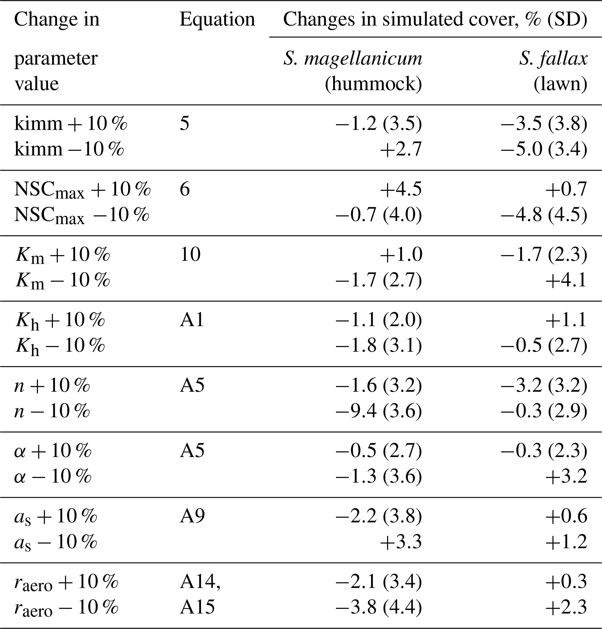
Table 3The results from Test 2, which addressed the robustness of the model to the uncertainties in a set of parameters. Each parameter was increased or decreased by 10 %. The model was run for S. magellanicum and S. fallax in their preferential habitats. The difference in mean cover between simulations as a function of changed or unchanged parameter values is given; the standard deviations (SD) of the means are given in parentheses. The parameters include the specific immobilization rate (kimm), the maximal nonstructural carbon (NSC) concentration (NSCmax), the hydraulic conductivity of the moss layer (Km), the hydraulic conductivity of the peat layer (Kh), the water retention parameters of the water retention curves (α and n), the snow layer surface albedo (as), and the aerodynamic resistance (raero).
Second, we tested the robustness of the model to the uncertainties in a set of parameters (tests 2–4). In Test 2, we focused on parameters that were closely linked to hydrology and growth calculations but were roughly parameterized (e.g. kimm, raero) or adopted as a priori from other studies (e.g. Ksat, α, n, NSCmax; see Table 2). One at a time, each parameter value was adjusted by +10 % or −10. A total of 40 Monte Carlo simulations were run using the same runtime settings as in Test 1. The simulated means of cover were then compared to those calculated without the parameter adjustment.
Tests 3 and 4 were then carried out to test whether the model could correctly predict the competitiveness of the species in dry and wet habitats if the species-specific trends in the capitulum water content were not correctly specified. For both species, we set the values of parameters controlling the water retention (i.e. Bcap and DS; Appendix B) and the water-stress effects on net photosynthesis (i.e. Wcap; Eq. 4) to be the same as those for S. magellanicum (Test 3) or same as those for S. fallax (Test 4). Our hypothesis would be supported if removing the interspecific differences in RWC responses led to the failure to predict the habitat preferences of the species.
We implemented tests 5 and 6 to investigate the importance of parameters that directly control the species ability to overgrow another species with a more rapid height increment (i.e. Pm20, Rs20, αPPFD, and Hspec) under lawn and hummock conditions. We eliminated the species differences in the parameter, so that the values were the same as those in S. magellanicum (Test 5) or the same as those in S. fallax (Test 6). The effects of the manipulation were compared with those from tests 3 and 4. For tests 3–6, 80 respective Monte Carlo simulations were run using the set-ups described in Test 1.
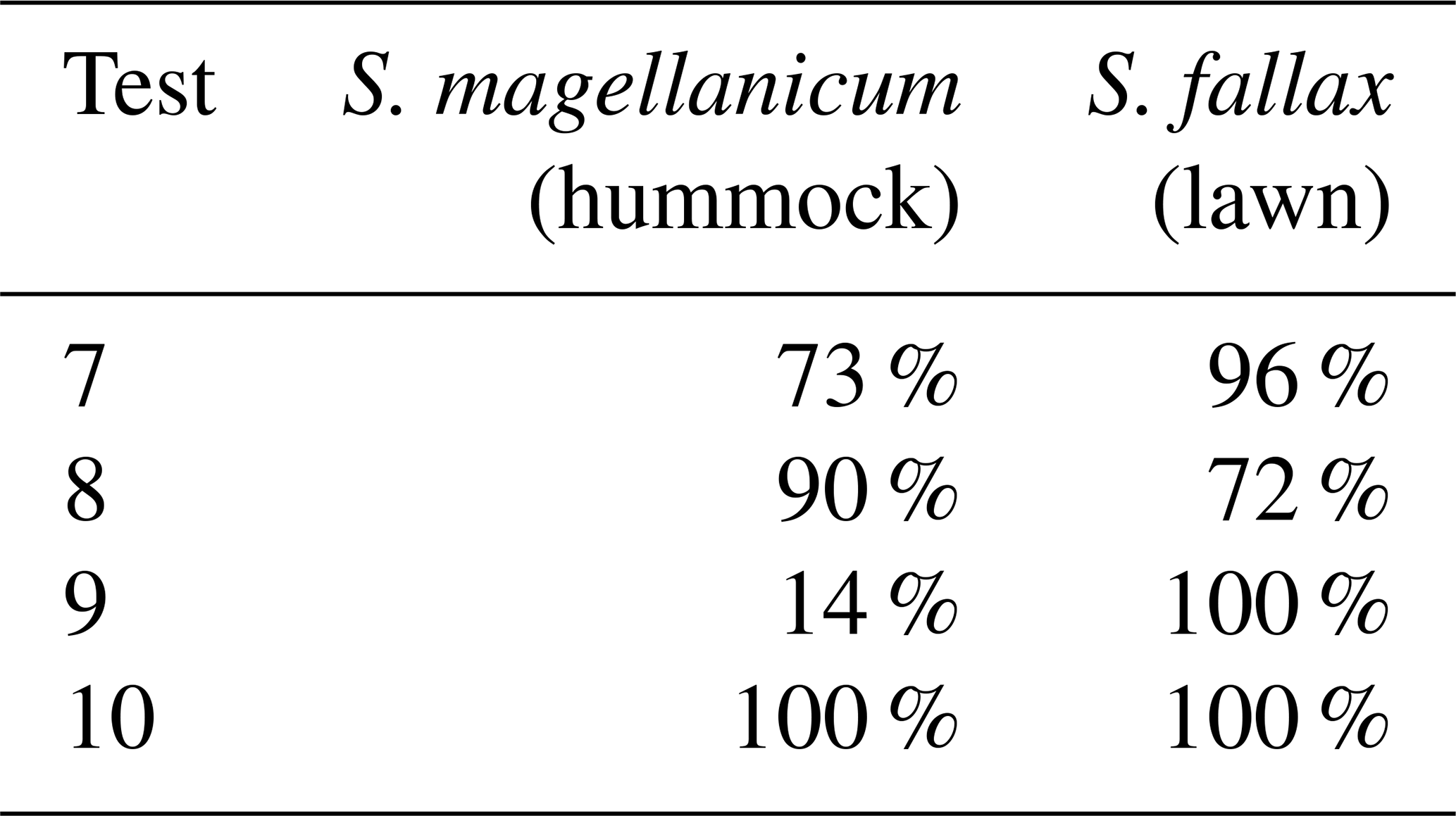
Tests 7 and 8 were implemented to separate the effects of photosynthetic water-response parameters from the effects of the capitula water retention. We set the photosynthetic water-response parameters to be the same as those in S. magellanicum (Test 7) or the same as those in S. fallax (Test 8). As our model aimed to couple the environmental fluctuations and stochasticity of ecosystem processes, we further tested the model responses to the absence of environmental fluctuations (Test 9) or the absence of stochasticity in model parameters (Test 10). In Test 9, monthly mean values of meteorological variables were used to drive the model simulation. In Test 10, we removed the stochasticity of model parameters and assigned an average value to each parameter of grid cells. For tests 7–10, 40 respective Monte Carlo simulations were run using the set-ups described in Test 1.
3.1 Simulating the habitat preferences of Sphagnum species as affected by the capitulum water content traits
Test 1 demonstrated the ability of the model to capture the preference of S. magellanicum for the hummock environment and the preference of S. fallax for the lawn environment (Fig. 2a). The simulated annual changes in species cover were greater in lawn habitats than in hummock habitats during the first 5 simulation years. The changes in lawn habitats slowed down around year 10, and the cover of S. fallax plateaued at around 95±2.8 % (mean ± standard error). In contrast, the cover of S. magellanicum on hummocks continued to grow until the end of the simulation and reached 83±3.1 %. In the lawn habitats, the cover of S. fallax increased in all Monte Carlo simulations, and the species occupied all grid cells in 70 % of the simulations. In the hummock habitats, the cover of S. magellanicum increased in 91 % of Monte Carlo simulations, and it formed a monocultural community in 16 % of simulations (Fig. 2b). The vertical growth of Sphagnum mosses was significantly greater in lawn habitats than in hummock habitats (P<0.01). The ranges of simulated vertical growth agreed well with the observed values from field measurement for both species (Fig. 2c).
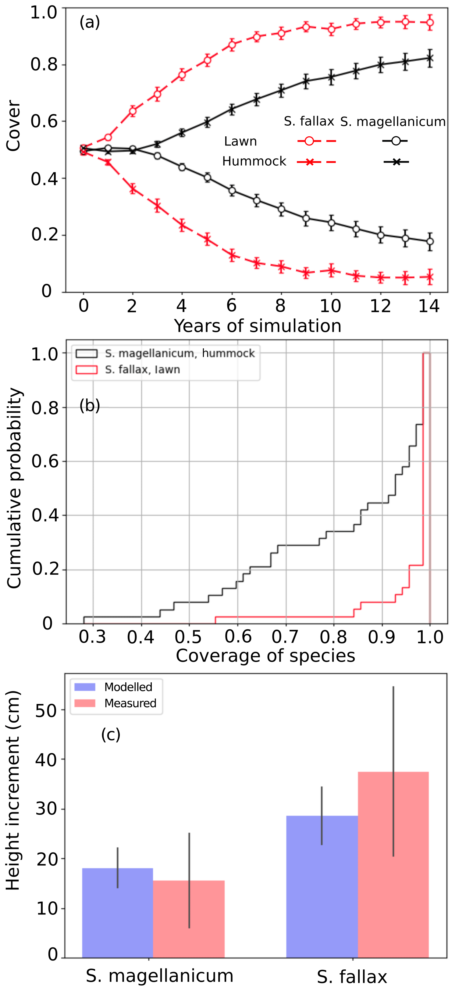
Figure 2Testing the ability of PMS to predict the habitat preference of Sphagnum magellanicum and S. fallax (Test 1). The hummock and lawn habitats were differentiated by the water table depth, the surface energy balances, and the capitulum water potential in the model simulations. At the beginning of the simulation, the cover of the two species was set to be equal and it was allowed to develop with time. (a) The annual development of the relative cover (mean and standard error) of the two species in hummock and lawn habitats, (b) the cumulative probability distribution of the cover of the two species at the end of the 15-year period based on 40 Monte Carlo simulations, and (c) the simulated and measured means of the annual vertical growth of Sphagnum surfaces in their natural habitats (hummock and lawn).
Table 4Result from tests 7–10, which addressed the importance of meteorological fluctuations, the stochasticity of model parameters, and the photosynthetic water response. In Test 7, monthly mean values of meteorological variables were used to drive the model simulation. In Test 8, the stochasticity of model parameters was removed, and the average values were used for parameters at the grid-cell level. In tests 9 and 10, the photosynthetic water-response parameters (i.e. aW0, aW1, and aW2; see Table 1) were set to be the same as those for S. magellanicum (Test 9) or the same as those for S. fallax (Test 10). The mean cover of S. magellanicum on hummocks and the cover of S. fallax on lawns after the 15-year simulation periods are listed in Table 4.
3.2 Testing model robustness
Test 2 addressed the model robustness to the uncertainties in several parameters that were closely linked to hydrology and growth calculations. Modifying most of the parameter values by +10 % or −10 % yielded marginal changes in the mean cover of species in either hummock or hollow habitats (Table 3). Reducing the moss carpet and the peat hydraulic parameter n had stronger impacts on S. fallax cover in hummock habitats than in lawn habitats. Nevertheless, changes in simulated cover that were caused by parameter manipulations were generally smaller than the standard deviations of the means, i.e. fitting into the random variation.
3.3 Testing the controlling role of the capitulum water content on community dynamics
In tests 3 and 4, the model incorrectly predicted the competitiveness of the two test species when the interspecific differences in the capitulum water content were eliminated. In both tests, S. fallax became dominant in all habitats. The use of water-response characteristics from S. magellanicum for both species (Test 3) led to the faster development of S. fallax cover and higher coverage at the end of simulation (Fig. 3a) compared with the simulation results where the water-response characteristics from S. fallax were used for both species (Test 4, Fig. 3b). The pattern was more pronounced in hummock than in lawn habitats.
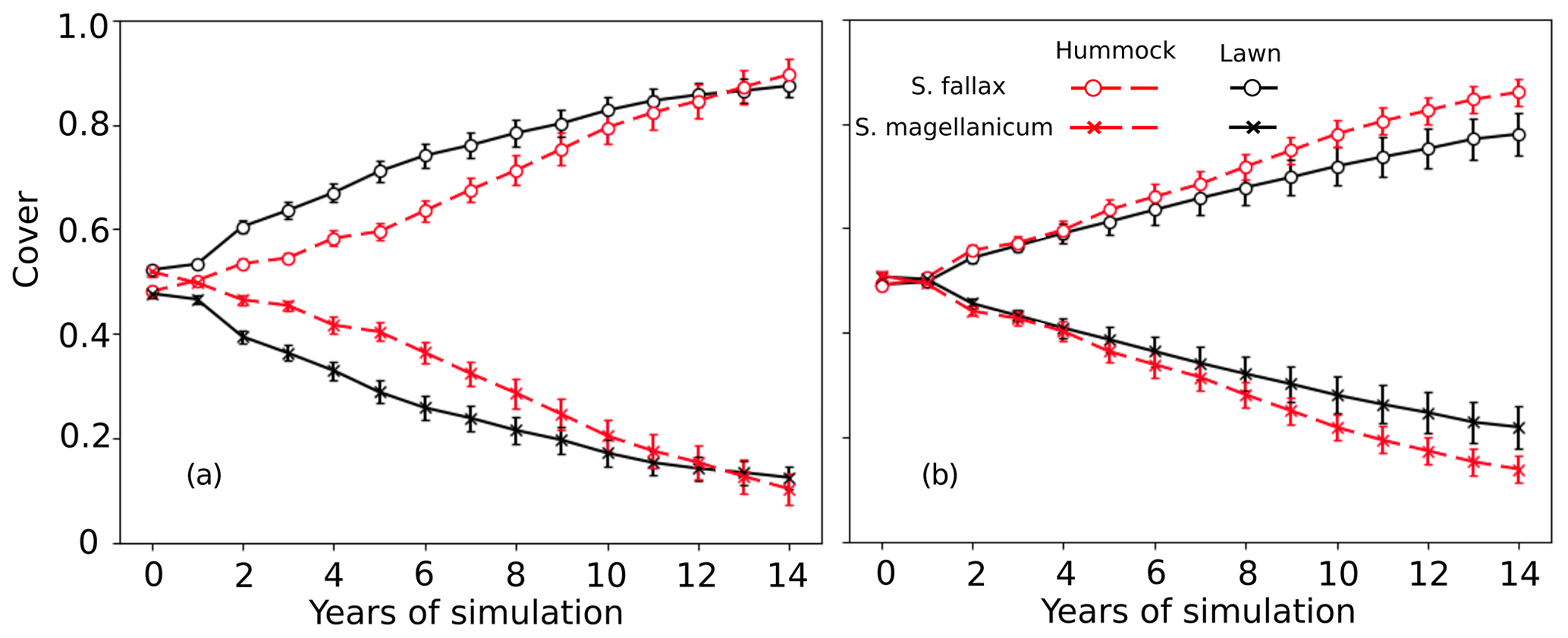
Figure 3Testing the importance of capitulum water content for the habitat preference of S. magellanicum and S. fallax. The development of the relative cover (mean and standard error) were simulated in hummock and lawn habitats over a 15-year time frame for the two species. For both species, parameter values for the capitulum water content, the capitulum biomass (Bcap), and the density (DS) were set to be the same as those from (a) S. magellanicum (Test 3) or (b) S. fallax (Test 4).
In tests 5 and 6, the species differences in the growth-related parameters were eliminated. However, the model still predicted the dominance of S. fallax and S. magellanicum in lawn and hummock habitats respectively (Fig. 4). The increase in the mean cover of S. magellanicum was especially fast in the hummock habitat in comparison to the results of the unchanged model from Test 1 (Fig. 2a). In lawns, the use of S. fallax growth parameters for both species gave stronger competitiveness to S. magellanicum (Fig. 4b) than using the S. magellanicum parameters (Fig. 4a). In tests 7 and 8, ignoring the interspecific differences in the photosynthetic water-response parameters did not change the simulated habitat preferences of S. fallax and S. magellanicum (Table 4). Using the water-response parameters of S. fallax decreased the mean cover of S. fallax in lawns but increased the cover of S. magellanicum on hummocks. In contrast, using the water-response parameters of S. magellanicum increased the mean cover of S. fallax in lawns but decreased the cover of S. magellanicum on hummocks.
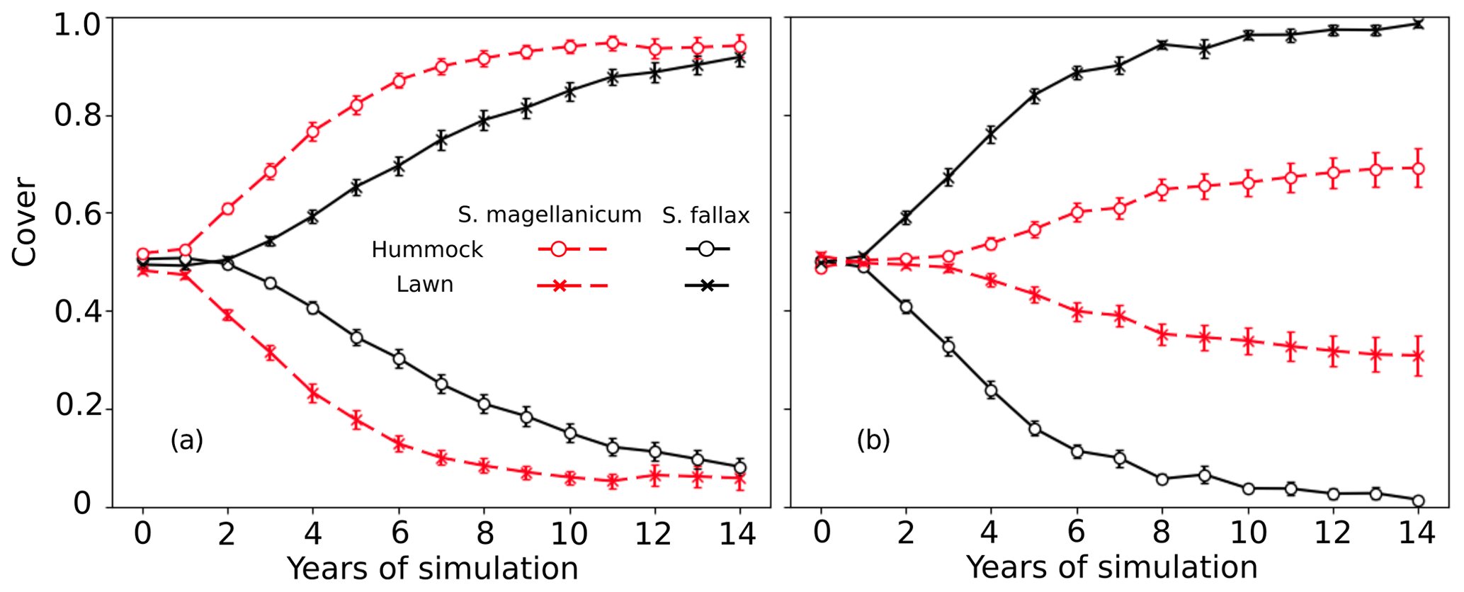
Figure 4Testing the importance of parameters regulating net photosynthesis and shoot elongation for the habitat preference of S. magellanicum and S. fallax. The annual development of the relative cover (mean and standard error) of the two species was simulated for hummock and lawn habitats over a 15-year time frame. For both species, the parameter values (i.e. Pm20, Rs20, αPPFD, and Hspec) were set to be the same as those from (a) S. magellanicum (Test 5) or (b) S. fallax (Test 6).
3.4 Testing the effects of environmental fluctuations and the stochasticity of ecosystem processes on community dynamics
In Test 9, the model failed to simulate the preference of S. magellanicum for hummocks (Table 4) if the environmental fluctuation was ignored. However, the simulated cover of S. fallax in lawns was higher compared with the unchanged condition (i.e. Test 1). Using the mean value for each model parameters led to monocultural community, i.e. S. magellanicum occupied 100 % of the hummock area whereas S. fallax took over lawns completely.
In peatland ecosystems, Sphagna are keystone species distributed primarily along the hydrological gradient (e.g. Andrus, 1986; Rydin, 1986). In a context where substantial change in peatland hydrology is expected under a changing climate in northern areas (e.g. longer snow-free season, lower summer water table, and more frequent droughts), there is a pressing need to understand how peatland plant communities could react and how Sphagnum species could redistribute under habitat changes. In this work, we developed the Peatland Moss Simulator (PMS), a process-based stochastic model, to simulate the competition between S. magellanicum and S. fallax, two key species representing dry (hummock) and wet (lawn) habitats in a poor fen peatland. We empirically showed that these two species differed in characteristics that likely affect their competitiveness along a moisture gradient.
Capitulum water retention for the lawn-preferring species (S. fallax) was weaker than that for the hummock-preferring species (S. magellanicum). Compared with S. magellanicum, the capitula of S. fallax held less water at saturation and the water content decreased more rapidly with dropping water potential. Hence, S. fallax would dry faster than S. magellanicum under the same rate of water loss. Moreover, the water content in S. fallax capitula was less resistant to evaporation. These differences indicated that it is harder for S. fallax capitula to buffer evaporative water loss and, therefore, avoid or delay desiccation. Similar differences between hummock and hollow species have been in previous studies (Titus and Wagner, 1984; Rydin and McDonald, 1985). In addition, the net photosynthesis of S. fallax is more sensitive to changes in the capitulum water content than S. magellanicum, as seen by the steeper decline in photosynthesis with decreasing water content (Fig. B2c). Consequently, the growth of S. fallax is more likely to be slowed down by dry periods, during which the capillary water cannot fully compensate for the evaporative loss (Robroek et al., 2007b), making it less competitive in habitats prone to desiccation.
The PMS successfully captured the habitat preferences of the two Sphagnum species (Test 1): starting from a mixed community with equal probabilities for both species, the lawn habitats with the shallower water table were eventually dominated by the typical lawn species S. fallax, whereas the hummock habitats, which were 15 cm higher than the lawn surface, were taken over by S. magellanicum. The low final cover of S. magellanicum simulated in lawn habitats agreed well with field observations from our study site, where S. magellanicum cover was less than 1 % in lawns (Kokkonen et al., 2019). Conversely, S. fallax was outcompeted by S. magellanicum in the hummock habitats. This result is consistent with previous findings that hollow-preferring Sphagna are less likely to survive in hummock environments with greater drought pressure (see Rydin, 1985; Rydin et al., 2006; Johnson et al., 2015). The simulated annual height increments of mosses also agreed well with the observed values for both habitat types. Our simulation for lawn habitat shows that the looser stem structure of S. fallax allows it to allocate more of its produced biomass into vertical growth and, therefore, overgrow S. magellanicum, in which new biomass forms a compact stem that is packed with thick fascicles. This finding indicates that PMS can capture the key mechanisms controlling the growth and competitive interactions of the Sphagnum species.
Parameter sensitivity testing showed the robustness of PMS regarding the uncertainties in parameterization, as the simulated changes in the mean species cover (under 10 % variation in several parameters) were generally less than the standard deviations of the means. Decreasing the value of the hydraulic parameter n (Table 2, Eq. A5) increased the presence of S. fallax in the hummock habitats. This was expected because n is a scaling factor and its changes are consequently magnified: a lower n value will lead to a higher water content in the unsaturated layers above the water table (van Genuchten, 1980), which allows Sphagna that are adapted to wet environments to survive dry conditions (Hayward and Clymo, 1982; Robroek et al., 2007b; Rice et al., 2008). In contrast, the response of Sphagnum cover to the changes in other hydraulic parameters (i.e. α, n, Kh) was limited in lawn habitats. This could be due to the relatively shallow water table in lawns, which was able to maintain sufficient capillary rise to the moss carpet and capitula. Decreasing the values of the specific immobilization rate (kimm) and maximal NSC concentration in Sphagnum biomass (NSCmax) mainly decreased the cover of S. fallax in lawn habitats, which is consistent with the importance of biomass production to Sphagna in high-moisture environments (e.g. Rice et al., 2008; Laine et al., 2011). In addition, the SVAT model simulations for hummocks and lawns (Module III, Fig. 1) employed the same hydraulic parameter values obtained from S. magellanicum hummocks (McCarter and Price, 2014). For lawns, this could overestimate Km but underestimate n, as the lawn peat would be less efficient at holding a high water content and generating capillary flow than hummock peat (Robroek et al., 2007b; Branham and Strack, 2014). As the decrease in Km and increase in n showed counteracting effects on the simulated species covers (Table 3), the biases in the parameterization of Km and n may not critically impact model performance.
Both our empirical measurements and PMS simulations indicate the importance of the capitulum water content as a mechanism for controlling the moss community dynamics in peatlands. The fact that the Sphagnum niche is defined by two processes has long been hypothesized and experimentally studied. Firstly, dry, high-elevation habitats such as hummocks physically select species with the ability to remain moist (Rydin, 1993). If the interspecific differences in water retention and water-stress effects were correctly specified (Test 1, Fig. 2) our model predicted this phenomena of stronger competitiveness of S. magellanicum with S. fallax in hummock habitats correctly. Alternatively, the model failed to predict the distribution of S. magellanicum on hummocks if these interspecific differences in the water processes were neglected (tests 3 and 4, Fig. 3). During low water table periods in summer, capillary rise may not fully compensate for high evaporation (Robroek et al., 2007b; Nijp et al., 2014). In such circumstances, the capitulum water potential could drop rapidly towards the pressure defined by the relative humidity of air (Hayward and Clymo, 1982). Consequently, the ability of capitula to retain cytoplasmic water is particularly important for the hummock-preferring species, as was also shown by Titus and Wagner (1984).
Secondly, in habitats with a more persistently high moisture content, such as lawns and hollows, interspecific competition becomes important: it is acknowledged that species from such habitats generally have higher growth rates and photosynthetic capacity than hummock species (e.g. Laing et al., 2014; Bengtsson et al., 2016). Our results also agreed with this, as setting the growth-related parameters (i.e. Pm20, Rs20, αPPFD, and Hspec) of S. magellanicum to be the same as those of S. fallax decreased the S. fallax cover in both hummock and lawn habitats (Test 6, Fig. 4b). However, such changes did not impact the simulated habitat preferences for the tested species. Based on this, the growth-related parameters seem to be less important than water-related parameters. Furthermore, tests 7 and 8 showed that when interspecific differences in the water-stress effects on photosynthesis were removed, the model still predicted correct habitat preferences for S. magellanicum and S. fallax. Therefore, the interspecific differences in the capitulum water retention could be the main determinant of the habitat preferences of the tested species.
There have been growing concerns about the shift of peatland communities from Sphagnum-dominated communities towards higher vascular abundance under a drier and warmer climate (Wullschleger et al., 2014; Munir et al., 2015; Dieleman et al., 2015). Nevertheless, the potential of the Sphagnum species composition to adjust to this forcing remains poorly understood. Particularly in oligotrophic fens, where the vegetation is substantially shaped by lateral hydrology (Tahvanainen, 2011; Turetsky et al., 2012), plant communities can be highly vulnerable to hydrological changes (Gunnarsson et al., 2002; Tahvanainen, 2011). Based on the validity and robustness of PMS, we believe that this model could serve as one of the first mechanistic tools to investigate the direction and rate of change in Sphagnum communities under environmental forcing. The hummock–lawn differences showed by Test 1 imply that S. magellanicum could outcompete S. fallax within a decade in a poor fen community if the water table of habitats such as lawns was lowered by 15 cm (Test 1). Although this was derived from a simplified system comprising only the two species, it highlighted the potential for rapid turnover of Sphagnum species: the hummock–lawn difference of the water table in the simulation was comparable to the expected water table drawdown in fens under a warming climate (Whittington and Price, 2006; Gong et al., 2012). The effect traits of mosses, while less studied than those of vascular plant traits, have far reaching impacts on the biogeochemistry of ecosystems such as peatlands, where mosses form the most significant plant group (Cornelissen et al., 2007). Due to the large interspecific differences of traits such as photosynthetic potential, hydraulic properties, and litter chemistry (Laiho, 2006; Straková et al., 2011; Korrensalo et al., 2017; Jassey and Signarbieux, 2019), a change in the Sphagnum community composition is likely to impact long-term peatland stability and functioning (Waddington et al., 2015). Turnover between hummock and wetter habitat species would feedback to climate, as they differ in their decomposability (Straková et al., 2012; Bengtsson et al., 2016). As hummock species produce more recalcitrant litter, the carbon bound in the system would take longer to be released back into atmosphere. In addition, the replacement of moss species that are adapted to wet conditions by hummock species is likely to result in a higher ability to maintain a carbon sink under periods of drought (Jassey, and Signarbieux, 2019).
Although efforts have been made in analytical modelling to obtain boundary conditions for equilibrium states of moss and vascular communities in peatland ecosystems (Pastor et al., 2002), the dynamic process of peatland vegetation has not been well described or included in Earth system models (ESMs). Existing ecosystem models usually consider the features of peatland moss cover as “fixed” (Sato et al., 2007; Wania et al., 2009; Euskirchen et al., 2014) or assume that they change directionally following a projected trajectory (Wu and Roulet, 2014). Chaudhary et al. (2017) presented a dynamic peatland vegetation model with a single moss PFT and four vascular PFTs so that moss productivity can vary relative to vascular plants; however, moss characteristics are fixed to a single set of values. Our modelling approach provided a way to incorporate the environmental fluctuation and the mechanisms of dynamic moss cover into peatland carbon modelling. PMS employed an individual-based approach in which each grid cell carries a unique set of trait properties; thus, shoots with favourable trait combinations in the prevailing environment are able to replace those whose trait combinations are less favourable. Moreover, the model included the spatial interactions of individuals, which can impact the sensitivity of the coexistence pattern to environmental changes (Bolker et al., 2003; Sato et al., 2007; Tatsumi et al., 2019). This mimics the stochasticity in plant responses to environmental fluctuations, which is essential for community assembly and trait filtering under environmental forcing (Clark et al., 2010). The importance of incorporating environmental fluctuations into the stochasticity of biophysiological processes is supported by tests 9 and 10. If the monthly mean climate conditions were used as input, our model failed to predict the dominance of S. magellanicum on hummocks. If the stochasticity of model parameters was omitted and only mean values were used, the model generated only single output that disregarded the randomness of environmental conditions. As these features are considered essential for “next-generation” dynamic vegetation models (DVMs; Scheiter et al., 2013), our PMS could be considered as an elemental design for future DVM development.
We see PMS as an elemental design for the future development of dynamic vegetation models for peatland ecosystems; however, there are certain uncertainties and features that should be developed further. We used a gas-exchange-based method to quantify the simultaneous changes in the capitula water potential, the water content, and the carbon uptake of Sphagnum moss capitula. It should be noted that the measurements mainly covered the changes from WCopt towards WCcmp (Appendix E and Fig. 3). However, the capitula water content could be higher than WCopt at saturation (e.g. about 25–30 g g−1; Schipperges and Rydin, 1998). When the RWC is high, vapour diffusion may occur mainly from the capitula surface or macropores (instead of the inside capitula). Hence, our methodology may not be suitable to reflect the water potential changes under near-saturated conditions. In our model simulations, we used the volumetric water content of the moss carpet to estimate the RWC as an approximation for wet conditions (Eq. 11). The accuracy of such an approximation for high RWC conditions remains ambiguous, and more information is still required. We assumed that tissue structure did not change during the measurement process and that the aerodynamic resistance (ra, Eq. 3) for vapour to diffuse from the inner capitula to the headspace was constant. However, capitula drying may change leaf curvature, especially in species with slim and sparsely spread leaves (Laine et al., 2018). Such changes in the branch-leaf structure could expose more of the leaf surface to evaporation and reduce the value of ra. Consequently, PMS could underestimate the capitula water potential towards the drying end for those species if a constant ra is derived from the maximal evaporation rate (Em, Eq. 5; Fig. 3c).
The water retention relationship in PMS may not sufficiently capture water potential changes at wet and dry extremes (e.g. S. magellanicum in Fig. 4c). Water retention functions developed for mineral soils (e.g. Clapp and Hornberge, 1978; van Genuchten, 1980) may not be well parameterized for peat soils and moss (nonvascular) vegetation, particularly under very dry or wet conditions. Hence, further studies are needed to improve the description of the nonlinearity of the capitula water content, as influenced by capitula morphology (e.g. capitula biomass and shoot density) and structural changes in leaves.
PMS lacks horizontal (lateral) water transport that may allow individuals from lawn species to be present on hummocks (Rydin, 1985). With additional experimental data, such as species-specific hydraulic conductivity, the current model could be improved to also quantify the horizontal water transport among neighbouring grid cells.
To conclude, PMS could successfully capture the habitat preferences of the modelled Sphagnum species. In this respect, PMS could provide fundamental support for the future development of dynamic vegetation models for peatland ecosystems. Based on our findings, capitulum water processes should be considered as a control on vegetation dynamics in future impact studies on peatlands under changing environmental conditions.
A1 Transport of water and heat in the peat profile
Simulating the transport of water and heat in the peat profiles was based on Gong et al. (2013). Here we list the key algorithms and parameters. Ordinary differential equations governing the vertical transport of water and heat in the peat profiles were given as follows:
where t is the time step; z is the thickness of the peat layer; h is the water potential; T is the temperature; Ch and CT are the specific capacity of water (i.e. ) and heat respectively; Kh and KT are the hydraulic conductivity and thermal conductivity respectively; and Sh and ST are the sink terms for water and energy respectively.
CT and KT were calculated as the volume-weighted sums from components of water, ice, and organic matter:
where Cwater, Cice, and Corg are the specific heats of water, ice, and organic matter respectively; Kwater, Kice, and Korg are the thermal conductivities of water, ice, and organic matter respectively; and θwater and θice are the volumetric contents of water and ice respectively.
For a given h, was derived from the van Genuchten water retention model (van Genuchten, 1980) as follows:
where θs is the saturated water content; θr is the permanent wilting point water content; α is a scale parameter that is inversely proportional to mean pore diameter; n is a shape parameter; and .
Hydraulic conductivity (Kh) in an unsaturated peat layer was calculated as a function of θ by combining the van Genuchten model with the Mualem model (Mualem, 1976):
where Ksat is the saturated hydraulic conductivity; Se is the saturation ratio, where ; and Le is the shape parameter (Le=0.5; Mualem, 1976).
A2 Boundary conditions and the surface energy balance
A zero-flow condition was assumed at the lower boundary of the peat column. The upper boundary condition was defined by the surface energy balance, which was driven by net radiation (Rn). The dynamics of Rn at surface x (x=0 for vascular canopy and x=1 for moss surface) was determined by the balance between incoming and outgoing radiation components:
where Rsnb,x and Rsnd,x are the absorbed energy from direct and diffuse radiation respectively; and Rlnx is the absorbed net longwave radiation.
Algorithms for calculating the net radiation components were detailed in Gong et al. (2013), as modified from the methods of Chen et al. (1999). Canopy light interception was determined by the light-extinction coefficient (klight), the leaf area index (Lc), and the solar zenith angle. The partitioning of reflected and absorbed irradiances at ground surface was regulated by the surface albedos for the shortwave (as) and longwave (al) components, and the temperature of surface x (Tx) also affects net longwave radiation:
where Rsib, Rsid, and Rli are the incoming beam, diffusive, and longwave radiation respectively; ε is the emissivity (); and δ is the Stefan–Boltzmann constant ( W m−2 K−4).
was partitioned into the latent heat flux (λEx), the sensible heat flux (Hx), and the ground heat flux (for canopy G1=0):
where Ts is the temperature of the moss carpet; and z is the thickness of the moss layer (z=5 cm).
The latent heat flux was calculated using the “interactive scheme” (Daamen and McNaughton, 2000; see also Gong et al., 2016), which is a K-theory-based, multisource model:
where Δ is the slope of the saturated vapour pressure curve against air temperature; λ is the latent heat of vaporization; E is the evaporation rate; VPDb is the vapour pressure deficit at zb; rb,x is the total resistance to water vapour flow, which is the sum of boundary layer resistance (rsa,x) and surface resistance (rss); and A is the available energy for evapotranspiration and Ax = – Gx.
The calculations of γ, λ, and VPDb require the temperature (Tb) and vapour pressure (eb) at the mean source height (zb). These variables were related to the total of latent heat (∑λEx) and sensible heat (∑Hx) from all surfaces using the Penman-type equations:
where ρaCp is the volumetric specific heat of air; raero is the aerodynamic resistance between zb and the reference height za and was a function of Tb accounting for the atmospheric stability (Choudhury and Monteith, 1988); and γ is the psychrometric constant ().
Changes in the energy balance affect the surface temperature (Tx) and vapour pressure (ex), which further feed back to the energy availability (Eqs. A10, A12), the source-height temperature, VPD, and the resistance parameters (e.g. raero). The values of Tx and ex were solved iteratively by coupling the energy balance equations (Eqs. A11–A15) with the Penman-type equations (see also Appendix B in Gong et al., 2016):
where the boundary layer resistance for ground surface (rsa,1) and canopy (rsa,0) were calculated following the approaches of Choudhury and Monteith (1988).
A3 Sink terms of transport functions for water and heat
The sink term Sh,i (see Eq. A11) for each soil layer i was calculated as follows:
where Ei is the evaporative loss of water from the layer; Pi is rainfall (Pi=0 if the layer is not the topmost layer, i.e. i<1); Wmelt,i is the amount of melt water added to the layer; and Ii is the net water inflow and was calibrated in Sect. 2.5.
The value of Ei was calculated as follows:
where E0 and E1 are the evaporation rate from the ground surface and canopy (Eq. A13) respectively; ftop is the location multiplier for the topmost layer (ftop=0 in cases i>1); and froot(i) is the fraction of fine-root biomass in layer i.
The value of Wmelt,i was controlled by the freeze–thaw dynamics of the soil water and snowpack, which were related to the heat diffusion in the soil profile (Eq. A2). We set the freezing point temperature to 0 ∘C, and the temperature of a soil layer was held constant (0 ∘C) during freezing or melting. For the ith soil layer, the sink term (ST) in the heat transport equation (Eq. A2) was calculated as follows:
where CT,i is the specific heat of the soil layer (Eq. A13); Wphase is the water content for freezing (Wphase=θw) or melting (Wphase=θice); λmelt is the latent heat of freezing; fphase is a binarial coefficient that denotes the existence of freezing or thawing. For each time step t, we computed Ti(t) with the prior assumption that 0. fphase was then determined by whether the temperature changed across the freezing point, i.e. fphase=1 if , otherwise fphase=0.
A4 Parameterization of SVAT processes
For the calculation of the surface energy balance, we set the height and leaf area of the vascular canopy to 0.4 m and 0.1 m2 m−2 respectively, which is consistent with the scarcity of vascular canopies at the site. The aerodynamic resistance (raero, Eq. A14, Appendix A) for surface energy fluxes was calculated following Gong et al. (2013a). The bulk surface resistance of the community (rss, Eq. A13, Appendix A) was summarized from the cell-level values of rbulk,i such that . To calculate the peat hydrology and water table, peat profiles of hummock and lawn communities were set to 150 cm deep and stratified into horizontal depth layers varying from 5 cm (topmost) to 30 cm (deepest). For each peat layer, the thermal conductivity (KT) of the fractional components, i.e. peat, water, and ice, were evaluated following Gong et al. (2013a). The bulk density of peat (ρbulk) was set to 0.06 g cm−3 below acrotelm (40 cm depth, Laine et al., 2004) and decreased linearly toward the living moss layer. The saturated hydraulic conductivity (Ksat, Eq. A6, Appendix A) and water retention parameters (i.e. α and n, Eq. A5, Appendix A) of water retention curves were calculated as functions of ρbulk and the depth of the peat layer following Päivänen (1973). Ksat, α, and n for the living moss layer were adopted from the values measured by McCarter and Price (2014) for S. magellanicum carpet. The parameter values for SVAT processes are listed in Table 3.
A5 Calculation of snow dynamics
In boreal and arctic regions, the amount and timing of snow melt has a crucial impact on moisture conditions, especially in fen peatlands. Therefore, in order to have realistic spring conditions, we introduced a snowpack model, SURFEX v7.2 (Vionnet et al., 2012) into the SVAT model simulations. The snowpack model simulates snow accumulation, wind drift, compaction, and changes in metamorphism and density. These processes influenced the heat transport and freezing–melting processes (i.e. Sh and ST, see Eqs. A1–A2 in Appendix A). In this model run, we calculate the snow dynamics on a daily basis in parallel to the SVAT simulation. Daily snowfall was converted into a snow layer and was added to ground surface. For each of the day-based snow layers (D-layers), we calculated the changes in snow density, particle morphology, and layer thicknesses. At each time step, D-layers were binned into layers with depths of 5–10 cm (S-layers) and placed on top of the peat column for SVAT model simulations. With a snow layer present, surface albedos (i.e. as and al) were modified to match those of the topmost snow layer (see Table 4 in Vionnet et al., 2007). If the total thickness of snow was less than 5 cm, all D-layers were binned into one S-layer. The thermal conductivity (KT), specific heat (CT), snow density, thickness, and water content of each S-layer were calculated as the mass-weighted means from the values of D-layers. Melting and refreezing tended to increase the density and KT of a snow layer but decrease its thickness (see Eq. 18 in Vionnet et al., 2007). The fraction of melted water that exceeded the water holding capacity of a D-layer (see Eq. 19 in Vionnet et al., 2007) was removed immediately as infiltration water. If the peat layer underneath was saturated, the infiltration water was removed from the system as lateral discharge.
A6 Boundary conditions and driving variables
A zero-flow boundary was set at the bottom of the peat. At the peat surface the boundary conditions of water and energy were defined by the ground surface temperature (T0, see Eqs. A10–A15 in Appendix A) and the net precipitation (P minus E). The profiles of layer thicknesses, ρbulk, and hydraulic parameters were assumed to be constant during simulation. Lateral boundary conditions were used to calculate the spreading of Sphagnum shoots among cells along the edge of the model domain so that shoots can spread across the edge of the simulation area and invade the grid cell at the boarder of the opposite side.
The model simulation was driven by the climatic variables of air temperature (Ta), precipitation (P), relative humidity (RH), wind speed (u), incoming shortwave radiation (Rs), and longwave radiation (Rl). To support the stochastic parameterization of the model and Monte Carlo simulations, the Weather Generator (Strandman et al., 1993) was used to generate randomized scenarios based on long-term weather statistics (period from 1981 to 2010) from the four closest weather stations of the Finnish Meteorological Institute. This generator had been intensively tested and applied under Finnish conditions (Kellomäki and Väisänen, 1997; Venäläinen et al., 2001; Alm et al., 2007). We also compared the simulated meteorological variables with 2 years of data measured from a Siikaneva peatland site (61∘50 N; 24∘10 E) that is located 10 km from our study site (Appendix C).
B1 Measurement of morphological traits
To quantify morphological traits, core (size: 7 cm diameter, 50 cm2 area, and a height of at least 8 cm) samples of S. fallax and S. magellanicum were collected at the end of August 2016, maintaining the natural density of the stand. Samples were stored in plastic bags in a cool room (4 ∘C) until analysis. Eight replicates were collected for each species. For each sample, the capitulum density (DS, shoots cm−2) was measured, and 10 moss shoots were randomly selected and separated into the capitula and stems (5 cm below the capitula). The capitula and stems were moistened and placed on tissue paper for 2 min to extract free-moving water, before they were weighed for the water-filled fresh weight. The samples were then dried at 60 ∘C for at least 48 h, and the dry masses were subsequently measured. The field-water contents of the capitula (Wcf, g g−1) and stems (Wsf, g g−1) were then calculated as the ratio of water to dry mass for each sample. The biomass of the capitula (Bcap, g m−2) and living stems (Bst, g m−2) was calculated by multiplying the dry mass by the capitulum density (DS). The biomass density of living stems (Hspc, g cm−1 m−2) was calculated by dividing Bst by the length of stems.
B2 Measurement of photosynthetic traits
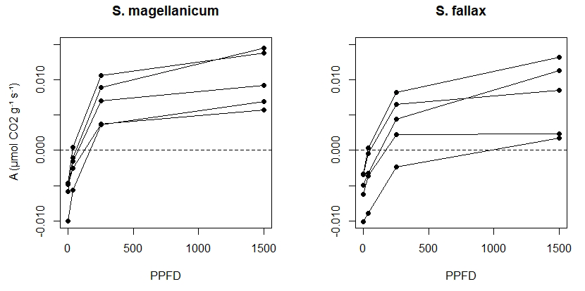
We measured the photosynthetic light response curves for S. fallax and S. magellanicum with fully controlled, flow-through gas-exchange fluorescence measurement systems (GFS-3000, Walz, Germany; Li-6400, LI-COR, US) under varying light levels. In 2016, measurements on field-collected samples were carried out during May and early June, which is a peak growth period for Sphagna (Korrensalo et al., 2017). Samples were collected from the field site each morning and were measured the same day at Hyytiälä field station. Samples were stored in plastic containers and moistened with peatland water to avoid changes in the plant status during the measurement. Right before the measurement, we separated Sphagnum capitula from their stems and dried them lightly using tissue paper before placing an even layer of them into a custom-made cuvette and retaining the same density as that found under natural field conditions (Korrensalo et al., 2017). The net photosynthesis rate (A, µmol g−1 s−1) was measured at 1500, 250, 35, and 0 µmol m−2 s−1 photosynthetic photon flux density (PPFD; Fig. 1b). The light levels were chosen based on previous investigation by Laine et al. (2011, 2015), which showed increasing A until PPFD at 1500 and no photoinhibition even at high values of 2000 µmol m−2 s−1. The samples were allowed to adjust to cuvette conditions before the first measurement and after each change in the PPFD level until the CO2 rate had reached a steady level, otherwise the cuvette conditions were kept constant (temperature 20 ∘C, CO2 concentration 400 ppm, flow rate 500 µmol s−1, impeller at level 5, and relative humidity of inflow air 60 %, although the relative humidity remained on average 81 % during the measurements). The time required for a full measurement cycle varied between 60 and 120 min. Each sample was weighed before and after the gas-exchange measurement and was then dried at 40 ∘C for 48 h to determine the biomass of capitula (Bcap). For each species, five samples were measured as replicates and were made to fit a hyperbolic light-saturation curve (Larcher, 2003):
where subscript 20 denotes the variable value measured at 20 ∘C; Rs is the mass-based dark respiration rate (µmol g−1 s−1); Pm is the mass-based rate of maximal gross photosynthesis (µmol g−1 s−1); and αPPFD is the half-saturation point (µmol m−2 s−1), i.e. the PPFD level where half of Pm is reached. The measured morphological and photosynthetic traits are listed in Table 2.
B3 Drying experiment
To link the water retention and photosynthesis of Sphagnum capitula, we performed a drying experiment using a GFS-3000 system to measure covariations of capitulum water potential (h, cm water), water content (Wcap, g g−1), and A (µmol g−1 s−1). For both species, four mesocosms were collected in August 2018 and transported to the laboratory at UEF Joensuu, Finland. Capitula were harvested and wetted by water from the mesocosms. The capitula were then placed gently onto a piece of tissue paper for 2 min before being placed into the same cuvette as that used in the previous photosynthesis measurement. The cuvette was then placed into the GFS-3000 and measured under constant PPFD (1500 µmol m−2 s−1), temperature (293.2 K), inflow air (700 µmol s−1), CO2 concentration (400 ppm), and relative humidity (40 %) conditions. Measurement was stopped when A dropped below 10 % of its maximum. Each measurement lasted between 120 and 180 min. Each sample was weighed before and after the gas-exchange measurement and then dried at 40∘C for 48 h to determine the biomass of capitula (Bcap).
The GFS-3000 records the vapour pressure (ea, kPa) and the evaporation rate (E, g s−1) simultaneously with A every second (Walz, Germany, 2012). The changes in Wcap with time (t) were calculated as follows:
We assumed that the vapour pressure at the surface of water-filled cells equaled the saturation vapour pressure (es), and the vapour pressure in the headspace of the cuvette equaled that in the outflow (ea). Thus, the vapour pressure in capitula pores (ei) can be calculated based on the following gradient-transport function (Fig. B2a):
where λ is the latent heat of vaporization; γ is the slope of the saturation vapour pressure–temperature relationship; ra is the aerodynamic resistance (m s−1) for vapour transport from the inter-leaf volume to the headspace; and rs is the surface resistance of vapour transport from the wet leaf surface to the inter-leaf volume. Thus, the bulk resistance for evaporation (rbulk) was calculated as ra+rs.
We assumed that the structures of the tissues and pores did not change during the drying process and that ra was constant during each measurement. A tended to increase with time t until it peaked (Am) and then subsequently decreased (Fig. 2b). The point A=Am implied the water content where further evaporative loss would start to drain the cytoplasmic water, leading to a decrease in A. The response of A to Wcap was fitted as a second-order polynomial function (Robroek et al., 2009) using data from to tn:
where aW0, aW1, and aW2 are parameters, and . For each replicate, the optimal water content for photosynthesis (Wopt) was derived from the peak of the fitted curve (Eq. 4). The capitulum water content at the compensation point Wcmp, where the rates of gross photosynthesis and respiration are equal, can be calculated from the point A=0.

Figure B2Conceptual schemes of (a) the cuvette setting and resistances, (b) the covariations of net photosynthesis and Wcap, and (c) the covariations of evaporation and vapour pressure in the headspace during a measurement. The symbols utilized in the figure are as follows: ea is the vapour pressure in the headspace of the cuvette (kPa); ei is the vapour pressure in the branch-leaf structure of the capitula; es is the vapour pressure at the surface of wet tissues; ra is the aerodynamic resistance of vapour diffusion from the inner capitula to the headspace; rs is the surface resistance of vapour diffusion from the wet tissue surface to the inner capitula space; A is the net photosynthesis rate (µmol m−2 s−1); Am is the maximal net photosynthesis rate (µmol m−2 s−1); Wcap is the water content of the capitula (g g−1); Wopt is Wcap at A=Am; Wcmp is Wcap at A=0; E is the evaporation rate (mm s−1).
Similarly, the evaporation rate (E) increased from the start of the measurement until the maximum evaporation Em and then decreased (Fig. B2c). The point E=Em implied the time when the wet capitulum tissues underwent maximum exposure to the air flow. Therefore, ra was estimated as the minimum of bulk resistance using Eq. (B5) and assuming ei(t)≈es when E(t)=Em:
Based on the calculated ei(t), we were able to derive the capitulum water potential (h) following the equilibrium vapour pressure method (e.g. Price et al, 2008; Goetz and Price, 2015):
where R is the universal gas constant (8.314 J mol−1 K−1); M the molar mass of water (0.018 kg mol−1); g is the gravitational acceleration (9.8 N kg−1); ei∕es is the relative humidity; and h0 is the water potential due to the emptying of free-moving water before measurement (set to 10 kPa according to Hayward and Clymo, 1982).
Table B1Species-specific morphological, photosynthetic, and water retention traits from S. magellanicum and S. fallax. Trait values (mean ± standard deviation) and ANOVA statistics, F and p values, are given to compare the mean values of traits for the two species.
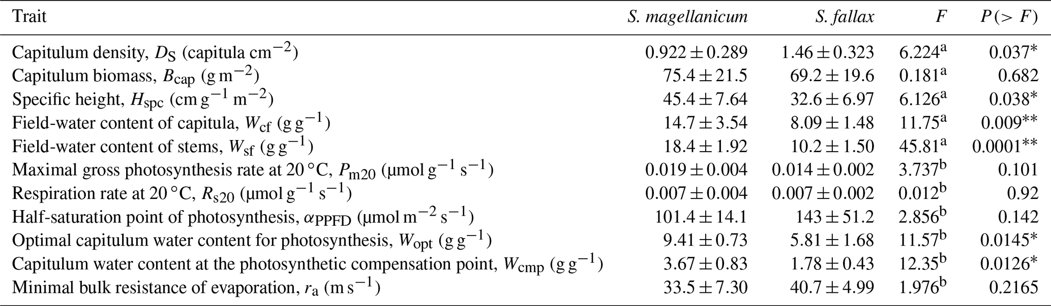
a Soil core measurement, sample n=5. b Cuvette gas-exchange measurement, sample n=4. ∗ The difference between the means is significant (P<0.05). The difference between the means is very significant (P<0.01).
Table B2Parameter estimates of the linear model for the log10-transformed capitulum water potential (h) for S. fallax and S. magellanicum. The estimated value, the standard error (SE), and the test statistics (p values) are given for the predictors of the models. The predictors are the capitulum biomass (Bcap), the capitulum density (DS), the capitulum water content (Wcap), the interaction of the capitulum biomass and water potential (Bcap×Wcap), the interaction of the capitulum biomass and capitulum density (DS×Wcap), the interaction of the capitulum density and water potential (DS×Wcap), and the interaction of the capitulum biomass, capitulum density, and water potential (). All coefficient values are significantly different from zero (p<0.001).
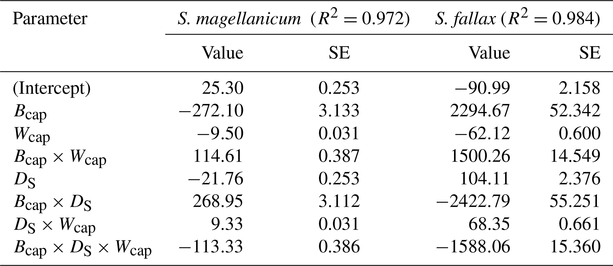
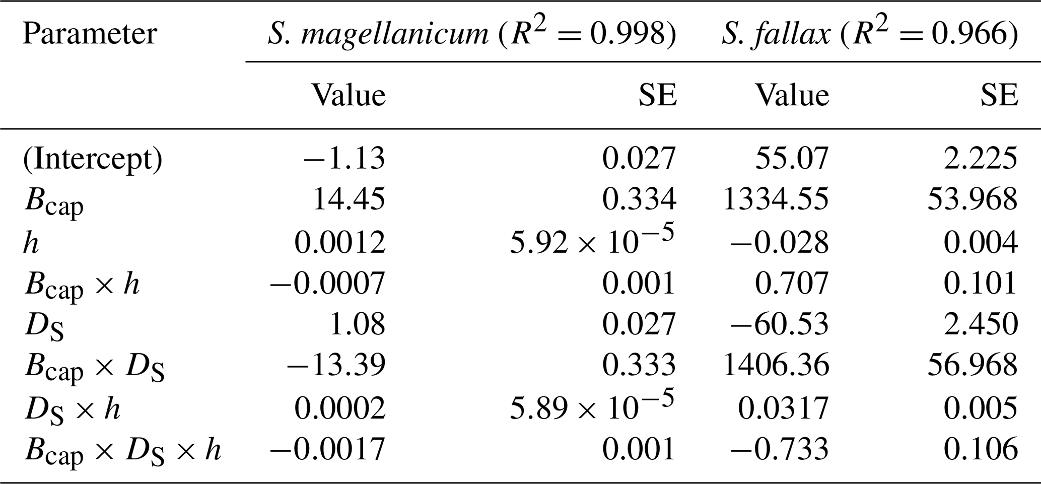
Table B3Parameter estimates of the linear model for the log10-transformed capitulum evaporative resistance (rbulk) for S. fallax and S. magellanicum. The estimated value, the standard error (SE), and the test statistics (p values) are given for the predictors of the models. The predictors are the capitulum biomass (Bcap), the capitulum density (DS), the water potential (h), the interaction of capitulum biomass and water potential (Bcap×h), the interaction of capitulum biomass and capitulum density (DS×h), the interaction of capitulum density and water potential (DS×h), and the interaction of capitulum biomass, capitulum density, and water potential (). All coefficient values are significantly different from zero (p<0.001).
B4 Statistical analysis
The light response curve (Eq. B1) and the response function of A∕Am to Wcap changes (Eq. B4) were fitted using the nlme package in R (version 3.1). The obtained values of the shape parameters aW0, aW1, and aW2 (Eq. 4) were then used to calculate Wopt () and Wcmp . We subsequently applied an ANOVA to compare S. magellanicum with S. fallax with respect to the traits obtained from the field sampling (i.e. structural properties such as Bcap, DS, Hspc, Wcf, and Wsf) and from the gas-exchange measurements (i.e. Pm20, Rs20, Wopt, Wcmp, and rbulk), using R (version 3.1).
The measured values of the capitulum water potential (h) were log10 transformed and related to the variations in Wcap, Bcap, and DS using a linear model. Similarly, a linear model was established to quantify the response of bulk resistance for evaporation (rbulk) (log10 transformed) to the variations in h, Bcap, and DS. The linear regressions were based on statsmodels (version 0.9.0) in Python (version 2.7), as supported by the NumPy (version 1.12.0) and pandas (version 0.23.4) packages.
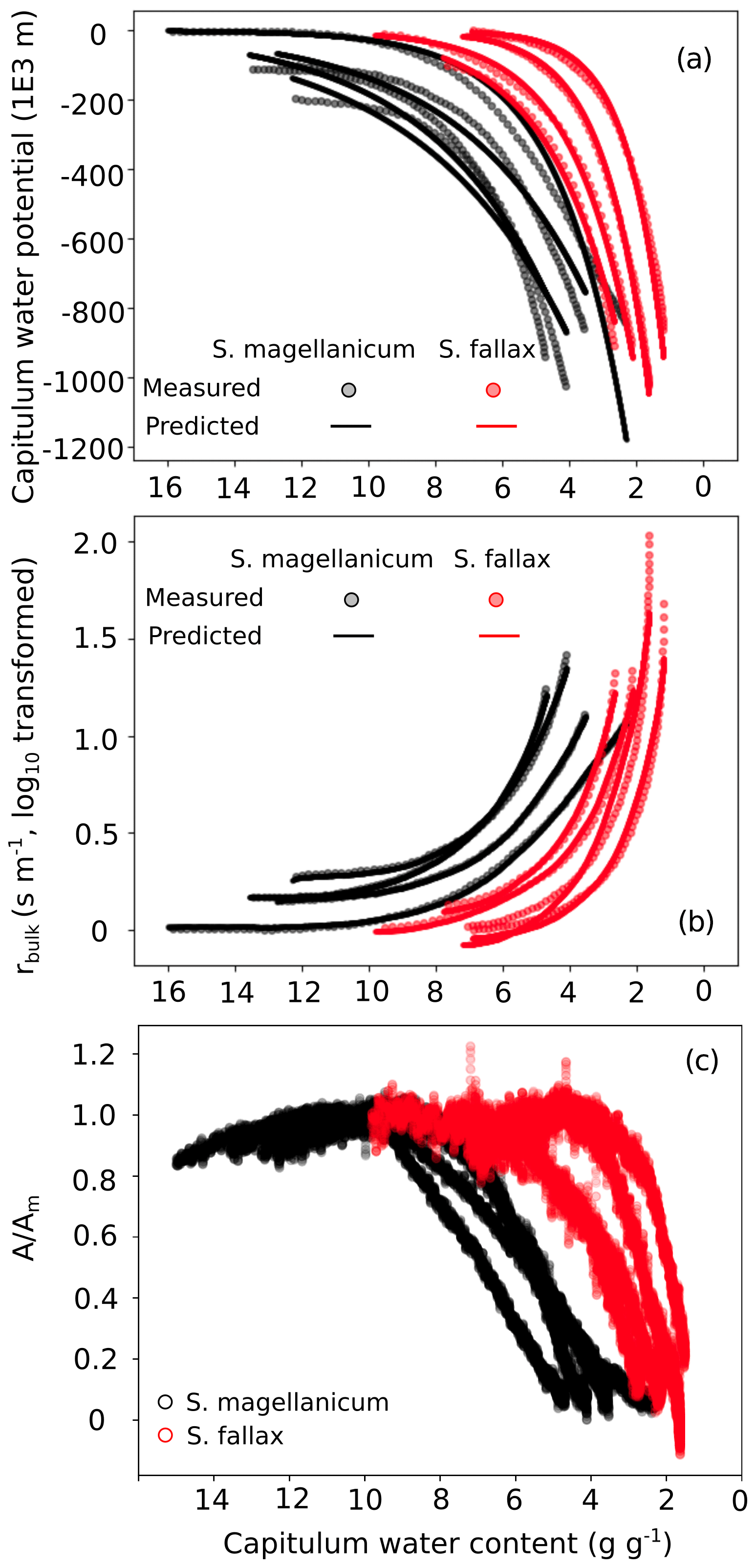
Figure B3Responses of (a) the capitulum water potential, (b) the bulk resistance of evaporation, and (c) the net photosynthesis to changes in the capitulum water content (Wcap) of two Sphagnum species typical to hummocks (S. magellanicum, black) and lawns (S. fallax, red). As the measured results are based on the drying experiment starting with fully wetted capitula characteristic for both species, the x axis is shown from high to low Wcap. The values predicted in panels (b) and (c) are based on linear models with the parameter values listed in Tables B2 and B3 and predictor values from the drying experiment.
B5 Results of the empirical measurements
The two Sphagnum species differed with respect their structural properties (Table B1). The lawn species S. fallax had a looser structure than the hummock species S. magellanicum, as seen by the lower capitulum density (DS) and specific height (Hspc) in S. fallax than in S. magellanicum (P<0.05, Table. B1). Moreover, under the conditions prevailing at the study site, S. fallax mosses were dryer than S. magellanicum; the field-water contents of the S. fallax capitulum (Wcf) and stem (Wsf) were 40 % and 46 % lower than S. magellanicum (P<0.01, Table B1) respectively. The different density of the capitulum of the two species, which also differed in their capitulum size, led to similar capitulum biomass (Bcap) (P=0.682) between S. fallax with small capitulum and S. magellanicum with large capitulum. Unlike the structural properties, maximal CO2 exchange rates (Pm20 and Rs20) did not differ between the two species (Table B1).
The drying experiment demonstrated how the capitulum water content regulated capitulum processes in both of the Sphagnum species studied (Fig. B3). Decreasing capitulum water content (Wcap) led to a decrease in the water potential (h), and the responses of h to Wcap varied among replicates (Fig. 3a). The values of Wcap for S. fallax were generally lower than those for S. magellanicum under the same water potentials. The fitted linear models explained over 95 % of the variation in the measured h for both species (Table B2), although the fitted responses of h to Wcap were slightly smoother than the measured responses, particularly for S. magellanicum (Fig. B3a). The responses of h to Wcap were significantly affected by the capitulum density (DS), the capitulum biomass (Bcap), and their interactions with Wcap (Table B2).
Decreasing capitulum water content (Wcap) and water potential (h) were associated with increasing bulk resistance for evaporation (rbulk, Fig. B3b), although the sensitivity of rbulk to h changes varied by replicate. The values of rbulk from S. fallax were largely lower than those from S. magellanicum when the capitulum water contents of the two species were similar. The fitted linear models explained the observed variations in the measured rbulk well for both species (Fig. 2b, Table B3). The variation in the response of rbulkto h was significantly affected by the capitulum density (DS), the capitulum biomass (Bcap), and their interactions with h (Table B3).
Decreasing capitulum water content (Wcap) slowed the net photosynthesis rate down (Fig. B2c), as represented by the decreasing ratio of A∕Am. S. fallax required a lower capitulum water content (Wcap) than S. magellanicum to reach photosynthetic maximum and the photosynthetic compensation point. However, the ranges of the capitulum water content from the photosynthetic maximum (Wopt) or field capacity (Wfc) to that at the compensation point (Wcmp) were smaller for S. fallax than for S. magellanicum. Hence, S. fallax had narrower transition zone for photosynthesis to respond to drying compared with S. magellanicum.

Figure C1Comparisons of meteorological variables simulated by the Weather Generator and those measured from a Siikaneva peatland site. The variables include (a) cumulative precipitation (mm), (b) incoming shortwave radiation (W m−2), (c) air temperature (∘C), and (d) relative humidity (%). These variables were measured and simulated at a 30 min timescale. The measurements were carried out from 2012 to 2013. Details about the site and measurements are given in Alekseychik et al. (2018). The measured seasonal dynamics of the meteorological variables were generally in line with the 95 % confidence intervals (CI) of the simulated values, which were calculated based on Monte Carlo simulations (n=5).

Figure D1Comparison of the seasonal water table (WT) measured at the Lakkasuo study site and the values simulated by the calibrated PMS. WT values were sampled weekly from the lawn habitats both in the field and in the model output. The weekly mean WT was measured during 2001, 2002, 2004, and 2016. The modelled means and standard deviations (SD) of the WT were based on 20 Monte Carlo simulations. The simulated seasonality of the mean WT generally followed the measured trends. The calibration reduced the sum of squared error (SSE, Eq. 12) from 199.5 () to 117.3. The calibrated values for aN and bN were and respectively (Eq. A18).
| Symbol | Description | Unit |
| A | Net photosynthesis rate | (µmol m−2 s−1) |
| Am | Maximal net photosynthesis rate | (µmol m−2 s−1) |
| αimm | Temperature constant for NSC immobilization | (–) |
| αPPFD | Half-saturation point of PPFD for photosynthesis | (µmol m−2 s−1) |
| Bcap | Capitulum biomass | (g m−2) |
| CT | Specific heat | (J K−1 kg−1) |
| DS | Capitulum density | (shoots cm−2) |
| dH | Annual vertical growth of Sphagnum mosses | (cm) |
| dWT | Hummock–lawn differences in the water table | (cm) |
| E | Rate of evaporation | (cm time step−1) |
| fW | Water content multiplier on the photosynthesis rate | (–) |
| fT | Temperature multiplier on the photosynthesis rate | (–) |
| h | Water potential | (cm) |
| Hc | Shoot height of Sphagnum mosses | (cm) |
| Hcap | Height of capitula | (cm) |
| Hspc | Biomass density of living Sphagnum stems | (g m−2 cm−1) |
| I | Rate of net inflow water | (cm) |
| kimm | Specific immobilization rate | (g g−1) |
| JDthaw | Julian day when thawing completed | (–) |
| Kh | Hydraulic conductivity of the peat layer | (cm s−1) |
| Km | Hydraulic conductivity of the moss layer | (cm s−1) |
| Ksat | Saturated hydraulic conductivity | (cm s−1) |
| KT | Thermal conductivity | (W m−1 K−1) |
| lc | Width of a grid cell in the simulation | (cm) |
| MB | Immobilized NSC to biomass production | (g) |
| NSCmax | Maximal NSC concentration in Sphagnum biomass | (g g−1) |
| P | Precipitation | (cm) |
| Pm | Mass-based rate of maximal gross photosynthesis | (µmol g−1 s−1) |
| PPFD | Photosynthetic photon flux density | (µmol m−2 s−1) |
| ρbulk | Bulk density of peat | (g cm−3) |
| raero | Aerodynamic resistance | (s m−1) |
| rbulk | Cell-level bulk surface resistance | (s m−1) |
| rss | Bulk surface resistance of community | (s m−1) |
| RH | Relative humidity | (%) |
| Rs | Mass-based respiration rate | (µmol g−1 s−1) |
| Rs | Incoming shortwave radiation | (W m−2) |
| Rl | Incoming longwave radiation | (W m−2) |
| Sc | Area of a cell in the model simulation | (m2) |
| simm | Multiplier for the temperature threshold | (–) |
| Svi | Evaporative area of a cell i | (cm2) |
| T | Capitulum temperature | (∘C) |
| Ta | Air temperature | (∘C) |
| Topt | Reference temperature of respiration (20 ∘C) | (∘C) |
| u | Wind speed | (m s−1) |
| Wcap | Capitulum water content | (g g−1) |
| Wcmp | Capitulum water content at the compensation point | (g g−1) |
| Wmax | Maximum water content of capitula | (g g−1) |
| Wopt | Optimal capitulum water content for photosynthesis | (g g−1) |
| Wcf | Field-water contents of the Sphagnum capitulum | (g g−1) |
| Wsf | Field-water contents of the Sphagnum stem | (g g−1) |
| WTm | Measured multiyear mean of the weekly water table | (cm) |
| WTs | Simulated multiyear mean of the weekly water table | (cm) |
| zm | Thickness of the living moss layer | (cm) |
| θm | Volumetric water content of the moss layer | (–) |
| θr | Permanent wilting point water content | (–) |
| θs | Saturated water content | (–) |
| Abbreviations | |
| Γ | Learning rate of gradient decedent algorithms |
| D-layer | Daily based snow layer |
| ICOS | Integrated Carbon Observation System |
| JD | Julian day |
| NSC | Nonstructural carbon |
| PMS | Peatland Moss Simulator |
| RWC | Capitulum water content |
| SD | Standard deviation |
| SE | Standard error |
| SSE | Sum of squared error |
| SVAT | Soil–vegetation–atmosphere transport |
| WT | Water table |
The data and the code to reproduce the analysis are available from the corresponding author upon request.
JG and EST designed the study. JG, AML, and NK conducted the experiment and analysis. JG, EST, NR, and SF designed the model. JG coded the model and conducted the model simulation and data analysis. JG and EST wrote the paper with contributions from all co-authors.
The authors declare that they have no conflict of interest.
The authors are grateful to Harri Strandman (University of Eastern Finland) for coding the Weather Generator.
This research has been supported by the Academy of Finland (project no. 287039), the US National Science Foundation (grant no. 1802825), the Kone Foundation, and the Fulbright-Saastamoinen Foundation.
This paper was edited by Michael Bahn and reviewed by Maaike Bader and two anonymous referees.
Alekseychik, P., Lindroth, A., Mammarella, I., Lund, M., Rinne, J., Kasurinen, V., Nilsson, M., Peichl, M., Lohila, A., Aurela, M., Laurila, T., Shurpali, N., Tuittila, E.-S., Martikainen, P. M., and Vesala, T.: Surface energy exchange in natural and managed Fennoscandian peatlands, Mires and Peat, 21, 1–26, https://doi.org/10.19189/MaP.2018.OMB.333, 2018.
Alm, J., Shurpali, N. J., Tuittila, E.-S., Laurila, T., Maljanen, M., Saarnio, S., and Minkkinen, K.: Methods for determining emission factors for the use of peat and peatlands – flux measurements and modelling, Boreal Environ. Res., 12, 85–100, 2007.
Amarasekare, P.: Competitive coexistence in spatially structured environments: A synthesis, Ecol. Lett., 6, 1109–1122, 2003.
Anderson K. and Neuhauser C.: Patterns in spatial simulations – are they real?, Ecol. Model., 155, 19–30, 2000.
Andrus R. E.: Some aspects of Sphagnum ecology, Can. J. Bot., 64, 416–426, 1986.
Asaeda, T. and Karunaratne, S.: Dynamic modelling of the growth of Phragmites australis: model description, Aquat. Bot., 67, 301–318, 2000.
Bengtsson, F., Granath, G., and Rydin, H.: Photosynthesis, growth, and decay traits in Sphagnum – a multispecies comparison, Ecol. Evol., 6, 3325–3341, 2016.
Blois, J. L., Williams, J. W., Fitzpatrick, M. C., Jackson, S. T., and Ferrier, S.: Space can substitute for time in predicting climate-change effects on biodiversity, P. Natl. Acad. Sci. USA, 110, 9374–9379, https://doi.org/10.1073/pnas.1220228110, 2013.
Bolker, B. M., Pacala, S. W., and Neuhauser, C.: Spatial dynamics in model plant communities: What do we really know?, Am. Nat., 162, 135–148, 2003.
Boulangeat, I., Svenning, J. C., Daufresne, T., Leblond, M., and Gravel, D.: The transient response of ecosystems to climate change is amplified by trophic interactions, Oikos, 127, 1822–1833, 2018.
Branham, J. E. and Strack, M.: Saturated hydraulic conductivity in Sphagnum-dominated peatlands: do microforms matter?, Hydrol. Process., 28, 4352–4362, 2014.
Chaudhary, N., Miller, P. A., and Smith, B.: Modelling Holocene peatland dynamics with an individual-based dynamic vegetation model, Biogeosciences, 14, 2571–2596, https://doi.org/10.5194/bg-14-2571-2017, 2017.
Chen, J. M., Liu, J., Cihlar, J., abd Goulden, M. L.: Daily canopy photosynthesis model through temporal and spatial scaling for remote sensing applications, Ecol. Modell., 124, 99–119, 1999.
Choudhury, B. J. and Monteith, J. L.: A four‐layer model for the heat budget of homogeneous land surfaces, Q. J. Roy. Meteor. Soc., 114, 373–398, 1988.
Clapp, R. B. and Hornberger, G. M.: Empirical equations for some soil hydraulic properties, Water Resour. Res., 14, 601–604, 1978.
Clark, J. S., Bell, D., Chu, C., Courbaud, B., Dietze, M., Hersh, M., HilleRisLambers, J., Ibanez, I., LaDeau, S., McMahon, S., Metcalf, J., Mohan, J., Moran, E., Pangle, L., Pearson, S., Salk, C., Shen, Z., Valle, D., and Wyckoff, P.: High-dimensional coexistence based on individual variation: a synthesis of evidence, Ecol. Monogr., 80, 569–608, 2010.
Clymo, R. S.: The growth of Sphagnum: Methods of measurement, J. Ecol., 58, 13–49, 1970.
Cornelissen, J. H., Lang, S. I., Soudzilovskaia, N. A., and During, H. J.: Comparative cryptogam ecology: a review of bryophyte and lichen traits that drive biogeochemistry, Ann. Botany, 99, 987–1001, 2007
Czárán, T. and Iwasa, Y.: Spatiotemporal models of population and community dynamics, Trends Ecol. Evol., 13, 294–295, 1998.
Daamen, C. C. and McNaughton, K. G.: Modeling energy fluxes from sparse canopies and understorys, Agronomy Journal, 92, 837–847, 2000.
Dieleman, C. M., Branfireun, B. A., Mclaughlin, J. W., and Lindo, Z.: Climate change drives a shift in peatland ecosystem plant community: Implications for ecosystem function and stability, Glob. Change Biol., 21, 388–395, 2015.
Euskirchen, E. S., Edgar, C. W., Turetsky, M. R., Waldrop, M. P., and Harden J. W.: Differential response of carbon fluxes to climate in three peatland ecosystems that vary in the presence and stability of permafrost, permafrost, J. Geophys. Res.-Biogeo., 119, 1576–1595, 2014.
Frolking, S., Roulet, N. T., Moore, T. R., Lafleur, T. M., Bubier, L. J., and Crill, P. M.: Modeling seasonal to annual carbon balance of Mer Bleue Bog, Ontario, Canada, Global Biogeochem. Cy., 16, 4-1-4-21, https://doi.org/10.1029/2001GB001457, 2002.
Gassmann, F., Klötzli, F., and Walther, G.: Simulation of observed types of dynamics of plants and plant communities, J. Veg. Sci., 11, 397–408, 2003.
Goetz, J. D. and Price, J. S.: Role of morphological structure and layering of Sphagnum and Tomenthypnum mosses on moss productivity and evaporation rates, Can. J. Soil Sci., 95, 109–124, 2015.
Gong, J., Wang, K., Kellomäki, S., Wang, K., Zhang, C., Martikainen, P. J. and Shurpali, N.: Modeling water table changes in boreal peatlands of Finland under changing climate conditions, Ecological Modelling, 244, 65–78, 2012.
Gong, J., Shurpali, N., Kellomäki, S., Wang, K., Salam, M. M., and Martikainen, P. J.: High sensitivity of peat moisture content to seasonal climate in a cutaway peatlandcultivated with a perennial crop (Phalaris arundinacea, L.): a modeling study, Agr. Forest Meteorol., 180, 225–235, 2013.
Gong, J., Jia, X., Zha, T., Wang, B., Kellomäki, S., and Peltola, H.: Modeling the effects of plant-interspace heterogeneity on water-energy balances in a semiarid ecosystem, Agr. Forest Meteorol., 221, 189–206, 2016.
Gorham, E.: Northern peatlands: Role in the carbon cycle and probable responses to climatic warming, Ecol. Appl., 1, 182–195, 1991.
Gunnarsson, U., Malmer, N., and Rydin, H.: Dynamics or constancy in Sphagnum dominated mire ecosystems?, A 40-year study, Ecography, 25, 685–704, 2002.
Hartmann, H. and Trumbore, S.: Understanding the roles of nonstructural carbohydrates in forest trees – from what we can measure to what we want to know, New Phytol., 211, 386–403, 2016.
Hájek, T. and Beckett, R. P.: Effect of water content components on desiccation and recovery in Sphagnum mosses, Ann. Bot., 101, 165–173, 2008.
Hayward P. M. and Clymo R. S.: Profiles of water content and pore size in Sphagnum and peat, and their relation to peat bog ecology, P. Roy. Soc. Lond. B Bio., 215, 299–325, 1982.
Hayward P. M. and Clymo R. S.: The growth of Sphagnum: experiments on, and simulation of, some effects of light flux and water-table depth, J. Ecol., 71, 845–863, 1983.
Holmgren, M., Lin, C., Murillo, J. E., Nieuwenhuis, A., Penninkhof, J., Sanders, N., Bart, T., Veen, H., Vasander, H., Vollebregt, M. E., and Limpens, J.: Positive shrub-tree interactions facilitate woody encroachment in boreal peatlands, J. Ecol., 103, 58–66, 2015.
Hugelius, G., Tarnocai, C., Broll, G., Canadell, J. G., Kuhry, P., and Swanson, D. K.: The Northern Circumpolar Soil Carbon Database: spatially distributed datasets of soil coverage and soil carbon storage in the northern permafrost regions, Earth Syst. Sci. Data, 5, 3–13, https://doi.org/10.5194/essd-5-3-2013, 2013.
Jassey, V. E. and Signarbieux, C.: Effects of climate warming on Sphagnum photosynthesis in peatlands depend on peat moisture and species-specific anatomical traits, Glob. Change Biol., 25, 3859–3870, 2019.
Johnson, M. G., Granath, G., Tahvanainen, T., Pouliot, R., Stenøien, H. K., Rochefort, L., Rydin, H., and Shaw, A. J.: Evolution of niche preference in Sphagnum peat mosses, Evolution, 69, 90–103, 2015.
Kellomäki, S. and Väisänen, H.: Modelling the dynamics of the forest ecosystem for climate change studies in the boreal conditions, Ecol. Model., 97, 121–140, 1997.
Keuper, F., Dorrepaal, E., Van Bodegom, P. M., Aerts, R., Van Logtestijn, R. S. P., Callaghan, T. V., and Cornelissen, J. H. C.: A Race for Space? How Sphagnum fuscum stabilizes vegetation composition during long-term climate manipulations, Glob. Change Biol., 17, 2162–2171, 2011.
Kokkonen, N., Laine, A., Laine, J., Vasander, H., Kurki, K., Gong, J., and Tuittila, E.-S.: Responses of peatland vegetation to 15-year water level drawdown as mediated by fertility level. J. Veg. Sci., 30, 1206–1216, 2019.
Korrensalo, A., Hájek, T., Vesala, T., Mehtätalo, L., and Tuittila, E. S.: Variation in photosynthetic properties among bog plants, Botany, 94, 1127–1139, 2016.
Korrensalo, A., Alekseychik, P., Hájek, T., Rinne, J., Vesala, T., Mehtätalo, L., Mammarella, I., and Tuittila, E.-S.: Species-specific temporal variation in photosynthesis as a moderator of peatland carbon sequestration, Biogeosciences, 14, 257–269, https://doi.org/10.5194/bg-14-257-2017, 2017.
Kyrkjeeide, M. O., Hassel, K., Flatberg, K. I., Shaw, A. J., Yousefi, N., and Stenøien, H. K. Spatial genetic structure of the abundant and widespread peatmoss Sphagnum magellanicum Brid, PLoS One, 11, e0148447, https://doi.org/10.1371/journal.pone.0148447, 2016.
Laiho, R.: Decomposition in peatlands: Reconciling seemingly contrasting results on the impacts of lowered water levels, Soil Biol. Biochem., 38, 2011–2024, 2006.
Laine, A. M. Juurola, E., Hájek, T., and Tuittila, E.-S.: Sphagnum growth and ecophysiology during mire succession, Oecologia, 167, 1115–1125, 2011.
Laine, J., Komulainen, V.-M., Laiho, R., Minkkinen, K., Rasinmaki, A., Sallantaus, T., Sarkkola, S., Silvan, N., Tolonen, K., Tuittila, E.-S., Vasander, H., and Päivänen, J.: Lakkasuo – a guide to mire ecosystem, Department of Forest Ecology Publications, University of Helsinki, 31, 123 pp, 2004.
Laine, J., Flatberg, K. I., Harju, P., Timonen, T., Minkkinen, K., Laine, A., Tuittila, E.-S., and Vasander, H.: Sphagnum Mosses – The Stars of European Mires, University of Helsinki Department of Forest Sciences, Sphagna Ky., 326 pp, 2018.
Laine J., Harju P., Timonen T., Laine A., Tuittila E.-S., Minkkinen K., and Vasander H.: The inticate beauty of Sphagnum mosses – a Finnish guide to identification (Univ Helsinki Dept Forest Ecol Publ 39), Department of Forest Ecology, University of Helsinki, Helsinki, 1–190, 2009.
Laine, A., Ehonen, S., Juurola, E., Mehtätalo, L., and Tuittila, E.-S.: Performance of late succession species along a chronosequence: Environment does not exclude Sphagnum fuscum from the early stages of mire development, J. Veget. Sci., 26, 291–301, https://doi.org/10.1111/jvs.12231, 2015.
Laing, C. G., Granath, G., Belyea, L. R., Allton K. E., and Rydin, H.: Tradeoffs and scaling of functional traits in Sphagnum as drivers of carbon cycling in peatlands, Oikos, 123, 817–828, 2014.
Larcher, W.: Physiological Plant Ecology: Ecophysiology and Stress Physiology of Functional Groups, Springer, 514 pp., 2003.
Letts, M. G., Roulet, N. T., and Comer, N. T.: Parametrization of peatland hydraulic properties for the Canadian land surface scheme, Atmos. Ocean, 38, 141–160, 2000.
Martínez-Vilalta, J., Sala, A., Asensio, D., Galiano, L., Hoch, G., Palacio, S., Piper, F. I., and Lloret, F.: Dynamics of non-structural carbohydrates in terrestrial plants: a global synthesis, Ecol. Monogr., 86, 495–516, 2016.
McCarter, C. P. R. and Price, J. S.: Ecohydrology of Sphagnum moss hummocks: mechanisms of capitula water supply and simulated effects of evaporation, Ecohydrology, 7, 33–44, 2014.
Mualem, Y.: A new model for predicting the hydraulic conductivity of unsaturated porous media, Water Resour. Res., 12, 513–522, 1976.
Munir, T. M., Perkins, M., Kaing, E., and Strack, M.: Carbon dioxide flux and net primary production of a boreal treed bog: Responses to warming and water-table-lowering simulations of climate change, Biogeosciences, 12, 1091–1111, https://doi.org/10.5194/bg-12-1091-2015, 2015.
Murray, K. J., Harley, P. C., Beyers, J., Walz, H., and Tenhunen, J. D.: Water content effects on photosynthetic response of Sphagnum mosses from the foothills of the Philip Smith Mountains, Alaska, Oecologia, 79, 244–250, 1989.
Nijp, J. J., Limpens, J., Metselaar, K., van der Zee, S. E. A. T. M., Berendse, F., and Robroek, B. J. M.: Can frequent precipitation moderate the impact of drought on peatmoss carbon uptake in northern peatlands?, New Phytol., 203, 70–80, 2014.
O'Neill, K. P.: Role of bryophyte-dominated ecosystems in the global carbon budget, in: Bryophyte biology, edited by: Shaw, A. J. and Goffi, B., Cambridge University Press, Cambridge, UK, 344–368, 2000.
Pastor, J., Peckham, B., Bridgham, S., Weltzin, J., and Chen J.: Plant community dynamics, nutrient cycling, and alternative stable equilibria in peatlands, American Naturalist, 160, 553–568, 2002.
Päivänen, J.: Hydraulic conductivity and water retention in peat soils, Acta Forestalia Fennica, 129, 1–69, 1973.
Price, J. S., Whittington, P. N., Elrick, D. E., Strack, M., Brunet, N., and Faux, E.: A method to determine unsaturated hydraulic conductivity in living and undecomposed moss, Soil Sci. Soc. Am. J., 72, 487–491, 2008.
Price, J. S. and Whittington, P. N.: Water flow in Sphagnum hummocks: Mesocosm measurements and modelling, J. Hydrol., 381, 333–340, 2010.
Rice, S. K., Aclander, L., and Hanson, D. T.: Do bryophyte shoot systems function like vascular plant leaves or canopies?, Functional trait relationships in Sphagnum mosses (Sphagnaceae), Am. J. Botany, 95, 1366–1374, 2008.
Riutta, T., Laine, J., Aurela, M., Rinne, J., Vesala, T., Laurila, T., Haapanala, S., Pihlatie, M., and Tuittila, E.-S.: Spatial variation in plant community functions regulates carbon gas dynamics in a boreal fen ecosystem, Tellus B, 59, 838–852, 2007.
Robroek, B. J. M., Limpens, J., Breeuwer, A., Crushell, P. H., and Schouten, M. G. C.: Interspecific competition between Sphagnum mosses at different water tables, Funct. Ecol., 21, 805–812, 2007a.
Robroek, B. J. M., Limpens, J., Breeuwer, A., van Ruijven, J., and Schouten, M. G. C.: Precipitation determines the persistence of hollow Sphagnum species on hummocks, Wetlands, 4, 979–986, 2007b.
Robroek, B. J. M., Schouten, M. G. C., Limpens, J., Berendse, F., and Poorter, H.: Interactive effects of water table and precipitation on net CO2 assimilation of three co-occurring Sphagnum mosses differing in distribution above the water table, Glob. Change Biol., 15, 680–691, 2009.
Ruder, S.: An overview of gradient descent optimization algorithms, CoRR, abs/1609.04747, 2016.
Runkle, B. R. K., Wille, C., Gažovič, M., Wilmking, M., and Kutzbach, L.: The surface energy balance and its drivers in a boreal peatland fen of northwestern Russia, J. Hydrol., 511, 359–373, 2014.
Rydin, H.: Interspecific competition between Sphagnum mosses on a raised bog, Oikos, 66, 413–423, 1993.
Rydin, H.: Effect of water level on desiccation of Sphagnum in relation to surrounding Sphagna, Oikos, 374–379, 1985.
Rydin, H.: Competition and niche separation in Sphagnum, Can. J. Botany, 64, 1817–1824, 1986.
Rydin, H.: Competition between Sphagnum species under controlled conditions, Bryologist, 100, 302–307, 1997.
Rydin, H. and McDonald, A. J. S.: Tolerance of Sphagnum to water level, J. Bryol., 13, 571–578, 1985.
Rydin, H., Gunnarsson, U., and Sundberg, S.: The role of Sphagnum in peatland development and persistence, in: Boreal peatland ecosystems, edited by: Wieder, R. K. and Vitt, D. H., 30 Ecological Studies Series, Springer Verlag, Berlin, 47–65, 2006.
Sato, H., Itoh, A., and Kohyama, T.: SEIB-DGVM: A new Dynamic Global Vegetation Model using a spatially explicit individual-based approach, Ecol. Model., 200, 279–307, 2007.
Scheiter, S., Langan, L., and Higgins, S. I.: Next-generation dynamic global vegetation models: learning from community ecology, New Phytol., 198, 957–969, 2013.
Schipperges, B. and Rydin, H.: Response of photosynthesis of Sphagnum species from contrasting microhabitats to tissue water content and repeated desiccation, New Phytol., 140, 677–684, 1998.
Smirnoff, N.: The carbohydrates of bryophytes in relation to desiccation tolerance, J. Bryology, 17, 185–191, 1992.
Straková, P., Niemi, R. M., Freeman, C., Peltoniemi, K., Toberman, H., Heiskanen, I., Fritze, H., and Laiho, R.: Litter type affects the activity of aerobic decomposers in a boreal peatland more than site nutrient and water table regimes, Biogeosciences, 8, 2741–2755, https://doi.org/10.5194/bg-8-2741-2011, 2011.
Straková, P., Penttilä, T., Laine, J., and Laiho, R.: Disentangling direct and indirect effects of water table drawdown on above-and belowground plant litter decomposition: consequences for accumulation of organic matter in boreal peatlands, Glob. Change Biol., 18, 322–335, 2012.
Strandman, H., Väisänen, H., and Kellomäki, S.: A procedure for generating synthetic weather records in conjunction of climatic scenario for modelling of ecological impacts of changing climate in boreal conditions, Ecol. Model., 70, 195–220, 1993.
Tahvanainen, T.: Abrupt ombrotrophication of a boreal aapa mire triggered by hydrological disturbance in the catchment, J. Ecol., 99, 404–415, 2011.
Tatsumi, S., Cadotte M. W., and Mori, A. S.: Individual-based models of community assembly: Neighbourhood competition drives phylogenetic community structure, J. Ecol., 107, 735–746, 2019.
Thompson, D. K., Baisley, A. S., and Waddington, J. M.: Seasonal variation in albedo and radiation exchange between a burned and unburned forested peatland: implications for peatland evaporation, Hydrol. Proc., 29, 3227–3235, 2015.
Titus, J. E. and Wagner, D. J.: Carbon balance for two Sphagnum mosses: water balance resolves a physiological paradox, Ecology, 65, 1765–1774, 1984.
Turetsky, M. R.: The role of bryophytes in carbon and nitrogen cycling, Bryologist, 106, 395–409, 2003.
Turetsky, M. R., Crow, S. E., Evans, R. J., Vitt, D. H., and Wieder, R. K.: Trade-offs in resource allocation among moss species control decomposition in boreal peatlands, J. Ecol., 96, 1297–1305, 2008.
Turetsky, M. R., Bond-Lamberty, B., Euskirchen, E., Talbot, J., Frolking, S., McGuire, A. D., and Tuittila, E.: The resilience and functional role of moss in boreal and arctic ecosystems, New Phytol., 196, 49–67, 2012.
van Gaalen, K. E., Flanagan, L. B., Peddle, D. R.: Photosynthesis, chlorophyll fluorescence and spectral reflectance in Sphagnum moss at varying water contents, Oecologia, 153, 19–28, 2007.
van Genuchten, M.: A closed-form equation for predicting the hydraulic conductivity of unsaturated soils, Soil Sci. Soc. Am. J., 44, 892–898, 1980.
Väliranta, M., Korhola, A., Seppä, H., Tuittila, E. S., Sarmaja-Korjonen, K., Laine, J., and Alm, J.: High-resolution reconstruction of wetness dynamics in a southern boreal raised bog, Finland, during the late Holocene: a quantitative approach, Holocene, 17, 1093–1107, 2007.
Venäläinen, A., Tuomenvirta, H., Lahtinen, R., and Heikinheimo, M.: The influence of climate warming on soil frost on snow-free surfaces in Finland, Climate Change, 50, 111–128, 2001.
Vionnet, V., Brun, E., Morin, S., Boone, A., Faroux, S., Le Moigne, P., Martin, E., and Willemet, J.-M.: The detailed snowpack scheme Crocus and its implementation in SURFEX v7.2, Geosci. Model Dev., 5, 773–791, https://doi.org/10.5194/gmd-5-773-2012, 2012.
Vitt, D. H.: Peatlands: Ecosystems dominated by bryophytes, in: Bryophyte biology, edited by: Shaw, A. J. and Goffi, B., Cambridge University Press, Cambridge, UK, 312–343, 2000.
Waddington, J. M., Morris, P. J., Kettridge, N., Granath, G., Thompson, D. K., and Moore, P. A.: Hydrological feedbacks in northern peatlands, Ecohydrology, 8, 113–127, 2015.
Wania, R., Ross, I., and Prentice, I. C.: Integrating peatlands and permafrost into a dynamic global vegetation model: 2. Evaluation and sensitivity of vegetation and carbon cycle processes, Global Biogeochem. Cy., 23, GB3015, https://doi.org/10.1029/2008GB003413, 2009.
Weiss, R., Alm, J., Laiho, R., and Laine, J.: Modeling moisture retention in peat soils, Soil Sci. Soc. Am. J., 62, 305–313, 1998.
Whittington, P. N. and Price, J. S.: The effects of water table draw-down (as a surrogate for climate change) on the hydrology of a fen peatland, Canada, Hydrol. Proc., 20, 3589–3600, 2006.
Wilson, P. G.: The relationship among micro-topographic variation, water table depth and biogeochemistry in an ombrotrophic bog, Master Thesis, Department of Geography McGill University, Montreal, Quebec, p. 103, 2012.
Wojtuń, B., Sendyk, A., and Martynia, D.: Sphagnum species along environmental gradients in mires of the Sudety Mountains (SW Poland), Boreal Environ. Res., 18, 74–88, 2003.
Wu, J. and Roulet, N. T.: Climate change reduces the capacity of northern peatlands to absorb the atmospheric carbon dioxide: The different responses of bogs and fens, Global Biogeochem. Cy., 28, 1005–1024, https://doi.org/10.1002/2014GB004845, 2014.
Wullschleger, S. D., Epstein, H. E., Box, E. O., Euskirchen, E. S., Goswami, S., Iversen, C. M., Kattge, J., Norby, R. J., van Bodegom, P. M., and Xu, X.: Plant functional types in Earth system models: past experiences and future directions for application of dynamic vegetation models in high-latitude ecosystems, Ann. Bot., 114, 1–16, 2014.
- Abstract
- Introduction
- Materials and methods
- Results
- Discussion
- Appendix A: Calculating the community SVAT scheme (Module III)
- Appendix B: Methods and results of the empirical study on Sphagnum capitula water retention as a controlling mechanism for peatland moss community dynamics
- Appendix C: Comparisons of meteorological variables simulated by the Weather Generator and those measured from a Siikaneva peatland site (Integrated Carbon Observation System site located 10 km from the Lakkasuo study site)
- Appendix D: Comparisons of the seasonal water table measured from the study site and the values simulated based on calibrated net inflow
- Appendix E: List of symbols and abbreviations.
- Code and data availability
- Author contributions
- Competing interests
- Acknowledgements
- Financial support
- Review statement
- References
- Supplement