Evaluating two soil carbon models within the global land surface model JSBACH using surface and spaceborne observations of atmospheric CO₂

The trajectories of soil carbon in our changing climate are of the utmost importance as soil is a substantial carbon reservoir with a large potential to impact the atmospheric carbon dioxide (CO₂) burden. Atmospheric CO₂ observations integrate all processes affecting carbon exchange between the surface and the atmosphere and therefore are suitable for carbon cycle model evaluation. In this study, we present a framework for how to use atmospheric CO₂ observations to evaluate two distinct soil carbon models (CBALANCE, CBA, and Yasso, YAS) that are implemented in a global land surface model (JSBACH). We transported the biospheric carbon fluxes obtained by JSBACH using the atmospheric transport model TM5 to obtain atmospheric CO₂. We then compared these results with surface observations from Global Atmosphere Watch stations, as well as with column XCO₂ retrievals from GOSAT (Greenhouse Gases Observing Satellite). The seasonal cycles of atmospheric CO₂ estimated by the two different soil models differed. The estimates from the CBALANCE soil model were more in line with the surface observations at low latitudes (0–45^∘ N) with only a 1 % bias in the seasonal cycle amplitude, whereas Yasso underestimated the seasonal cycle amplitude in this region by 32 %. Yasso, on the other hand, gave more realistic seasonal cycle amplitudes of CO₂ at northern boreal sites (north of 45^∘ N) with an underestimation of 15 % compared to a 30 % overestimation by CBALANCE. Generally, the estimates from CBALANCE were more successful in capturing the seasonal patterns and seasonal cycle amplitudes of atmospheric CO₂ even though it overestimated soil carbon stocks by 225 % (compared to an underestimation of 36 % by Yasso), and its estimations of the global distribution of soil carbon stocks were unrealistic. The reasons for these differences in the results are related to the different environmental drivers and their functional dependencies on the two soil carbon models. In the tropics, heterotrophic respiration in the Yasso model increased earlier in the season since it is driven by precipitation instead of soil moisture, as in CBALANCE. In temperate and boreal regions, the role of temperature is more dominant. There, heterotrophic respiration from the Yasso model had a larger seasonal amplitude, which is driven by air temperature, compared to CBALANCE, which is driven by soil temperature. The results underline the importance of using sub-annual data in the development of soil carbon models when they are used at shorter than annual timescales.

1 Introduction

The terrestrial carbon cycle consists of the uptake of CO₂ by vegetation for photosynthesis and release of carbon by plants' autotrophic respiration, soil decomposition by heterotrophic organisms and natural disturbances (Bond-Lamberty et al., 2016). Soils store twice as much carbon as the atmosphere (Scharlemann et al., 2014), and its fate in a changing climate remains uncertain (Crowther et al., 2016). For example, while Crowther et al. (2016) concluded from a data-based analysis that large carbon stocks will lose more carbon due to warming conditions, van Gestel et al. (2018) questioned this view with an analysis based on a more comprehensive dataset. To have reliable predictions of future carbon stocks, a process-based understanding of the below-ground carbon cycle is needed (Bradford et al., 2016).

One way to evaluate soil carbon models has been to use observations of soil carbon stocks (Todd-Brown et al., 2013). At small scales, rates of gas exchange measured in chambers have also been used (Ťupek et al., 2019), but the separation of heterotrophic and autotrophic respiration is laborious (Chemidlin Prévost-Bouré et al., 2010). It is anyhow challenging to find reasons for differences in heterotrophic respiration between large-scale models as the litter input to the soil influences heterotrophic respiration, and this litter input varies between the models. One way forward is to use a test bed for these models, as done by Wieder et al. (2018).

An alternative, regionally integrated approach is using observations of atmospheric CO₂ which integrate all processes involved in global surface–atmosphere carbon exchange. The surface observation network of atmospheric CO₂ has been used in benchmarking global carbon cycle models (Cadule et al., 2010; Dalmonech and Zaehle, 2013; Peng et al., 2015). Recent advances of satellite technology have enabled retrievals of space-born, dry-air, total column-averaged CO₂ mole fraction (XCO₂), quantifying CO₂ in the entire atmospheric column between the land surface and the top of the atmosphere. These observations reveal a more spatially integrated CO₂ signal compared to surface site observations, and together they provide a complementary dataset. These two data sources have been used together to study the carbon cycle with “top-down” inversion modelling (Crowell et al., 2019). This kind of modelling framework uses atmospheric CO₂ observations to constrain a priori biospheric and ocean fluxes based on the Bayesian inversion technique, which results in optimised estimates (a posteriori) of the fluxes (Maksyutov et al., 2013; Rödenbeck et al., 2003; van der Laan-Luijkx et al., 2017; Wang et al., 2019). Estimates for fossil emissions are often assumed to be known, i.e. not optimised in the inversion.

In this study, we present a framework of how to use atmospheric CO₂ observations to evaluate soil carbon models implemented in a land surface model. We apply this to two state-of-the-art soil carbon models as a “proof of concept” for a more universal application. Basile et al. (2020) did similar work within a biogeochemical test bed and concluded that heterotrophic respiration can be a valuable benchmark in carbon cycle studies. They emphasised that the seasonal phasing of heterotrophic respiration relative to the net primary production (NPP) influences the net ecosystem exchange (NEE) and therefore potentially introduces bias to atmospheric CO₂ that hampers its use as a benchmark.

To obtain the atmospheric CO₂ profiles from our simulations with the land surface model, we applied an atmospheric transport model. In this work, we used the three-dimensional atmospheric chemistry transport model TM5 (Krol et al., 2005; Huijnen et al., 2010). Generally, transport models like TM5 contain errors caused by, for example, poorly resolved advection and heavily parameterised transport schemes (Gaubert et al., 2019). With TM5, we calculated the column-averaged CO₂ that can be used to evaluate model results versus the satellite observations. Satellite observations can also include errors. The uncertainty of GOSAT (Greenhouse Gases Observing Satellite) observations has been estimated to be around 1 to 2 ppm (Oshchepkov et al., 2013; Reuter et al., 2013). Contributors to uncertainties in the retrieval algorithms originate, for example, from the solar radiation database and the handling of aerosol scattering (Yoshida et al., 2013). Lastly, the column XCO₂ profiles are also influenced by, for example, advection and global-scale gradients driven by weather systems (Keppel-Aleks et al., 2011). A model evaluation performed with the column XCO₂ observations enabled a more thorough study of the fluxes and atmospheric physics of a modelling system (Keppel-Aleks et al., 2011).

We use in this work JSBACH, the land surface model of the Max Planck Institute's Earth system model, one of the models participating in CMIP6. The JSBACH model has two distinct soil models implemented in it (CBALANCE, CBA, and Yasso, YAS). We are interested in seeing if the two soil carbon models lead to markedly different CO₂ signals and in exploring which conclusions on model performance and process representation can be drawn that could help to improve this land surface model (and potentially other similar models) and our understanding of the land carbon cycle. The two model versions only differ with respect to the underlying soil processes and do not include major feedbacks between soil and vegetation (apart from a small effect of litter accumulation on fire emissions). Thus, the difference in the release of carbon to the atmosphere originates only from the soil carbon models. The two soil carbon models are both first-order decay models. However, they have different pool structures, as well as environmental drivers, and have differing response functions. CBALANCE uses soil moisture and soil temperature as driving variables, and Yasso uses precipitation and air temperature. In the analysis, we also use a simple box model calculation to further understand the main causes in the different outcomes of the models. Our framework combining a land surface model with a transport model allows us to investigate how these above-mentioned differences in soil carbon models influence atmospheric CO₂. Specifically, we aim to answer the following questions.

• How can we use a land surface model together with a transport model to evaluate soil carbon models and what problems do we face when doing that?

• What is the role of soil carbon stocks, the variables driving their decomposition and the functional dependencies of those variables on modelled heterotrophic respiration at global scale and how does this lead to differences in the atmospheric CO₂ signal?

2 Materials and methods

We used the land surface model JSBACH (Giorgetta et al., 2013) to obtain net land–atmosphere CO₂ exchange and fed that, together with ocean, fossil and land use fluxes, into a transport model, TM5, which simulates the resulting atmospheric CO₂ at selected surface sites, as well as column integrated values, for a comparison with satellite-derived column CO₂.

2.1 Model simulations: JSBACH with two soil carbon models

JSBACH is the global land surface model of the Max Planck Institute's Earth system model (Giorgetta et al., 2013), simulating terrestrial carbon, energy and water cycles (Reick et al., 2013). In this study, JSBACH was run with two different soil carbon sub-models that are described below. The older model, CBALANCE, has been used in Coupled Model Intercomparison Project Phase 5 (CMIP5) simulations of JSBACH (Giorgetta et al., 2013). The newer model, Yasso, has been used in simulations for the annual global carbon budget (Le Quéré et al., 2015, 2018) and is used in CMIP6 simulations of JSBACH (Mauritsen et al., 2019). It is also used in JSBACH4, a re-implementation of JSBACH for the ICOsahedral Non-hydrostatic Earth system model (ICON-ESM) (Giorgetta et al., 2018; Nabel et al., 2019).

Independent of the sub-model used for soil carbon, JSBACH uses three carbon pools for living vegetation: a wood pool containing woody parts of plants and green and reserve pools that contain the non-woody parts. JSBACH simulates different processes that lead to losses from the vegetation pools, such as grazing, shedding of leaves, and natural or anthropogenic disturbances. Depending on the process, some of the vegetation carbon is lost as CO₂ into the atmosphere, while the remaining part is transferred as dead vegetation into the litter and soil pools of the sub-model for soil carbon, where it is then subject to the internal processes of the soil carbon sub-model. The only process outside of the soil carbon sub-model that influences dead material is fire which burns parts of above-ground litter carbon.

2.1.1 The soil carbon model CBALANCE

CBALANCE (CBA) is the original soil carbon sub-model of JSBACH (Raddatz et al., 2007), which has been used in CMIP5. The environmental drivers for decomposition in CBA are soil temperature (at soil depths of 30 to 120 cm below the surface) and relative soil moisture, α, of the upper-most soil layer, which is 5 cm thick. The value of α varies between 0 and 1.

The function for soil temperature dependence, $f_{\mathrm{CBA},T_{\mathrm{soil}}}$, of decomposition follows a Q₁₀ formulation as follows:

$$\begin{array}{}\text{(1)}& f_{\mathrm{CBA},T_{\mathrm{soil}}}\left(T_{\mathrm{soil}}\right)=Q_{\mathrm{10}}^{\frac{T_{\mathrm{soil}}}{\mathrm{10}{}^{\circ }\mathrm{C}}},\end{array}$$

with a Q₁₀ value of 1.8 and T_soil as soil temperature (in ^∘C) (shown in Fig. S1a in the Supplement) (Raddatz et al., 2007). The dependency on relative soil moisture α is linear (Fig. S1b), and it is calculated as follows:

$$\begin{array}{}\text{(2)}& f_{\mathrm{CBA},\mathit{\alpha }}\left(\mathit{\alpha }\right)=\mathrm{MAX}\left({\mathit{\alpha }}_{min},{\displaystyle \frac{\mathit{\alpha }-{\mathit{\alpha }}_{\mathrm{crit}}}{\mathrm{1.0}-{\mathit{\alpha }}_{\mathrm{crit}}}}\right),\end{array}$$

where α_crit is 0.35 and α_min is 0.1 (Knorr, 2000).

Together these functions are modulating the rate of decomposition so that the heterotrophic respiration (R_h) from each pool (denoted by i) is as follows:

$$\begin{array}{}\text{(3)}& R_{\mathrm{h}}(T_{\mathrm{soil}},\mathit{\alpha })=f_{\mathrm{CBA},\mathit{\alpha }}\cdot f_{\mathrm{CBA},T_{\mathrm{soil}}}\cdot {\displaystyle \frac{C_i}{{\mathit{\tau }}_i}},\end{array}$$

where C_i is the carbon content of each pool and τ_i is the turnover time of each pool in days. CBA uses five different carbon pools having different turnover times:

• two green litter pools, one above ground and one below ground, in which the non-woody plant parts decompose with turnover times of between 1.8 and 2.5 years (Goll et al., 2015);

• two woody litter pools, one above ground and one below ground, in which the woody plant parts decompose with turnover times of several decades;

• one slow pool receiving its input from the four litter pools and having a turnover time in the order of a century.

2.1.2 The soil carbon model Yasso

The original soil carbon model of JSBACH was replaced by Yasso (YAS) (Thum et al., 2011; Goll et al., 2015). JSBACH's YAS implementation is based on the Yasso07 model (Tuomi et al., 2009). Development of Yasso07 relied heavily on litter bag and other observational datasets that were used to estimate model parameters (Tuomi et al., 2009, 2011). Owing to its strong connection to experiments, its environmental drivers are quasi-monthly air temperature and precipitation.

The decomposition dependency on air temperature is as follows:

$$\begin{array}{}\text{(4)}& f_{\text{YAS},T_{\text{air}}}\left(T_{\text{air}}\right)=e^{{\mathit{\beta }}_{\mathrm{1}}{T}_{\text{air}}+{\mathit{\beta }}_{\mathrm{2}}{T}_{\text{air}}^{\mathrm{2}}},\end{array}$$

where T_air is air temperature (^∘C), parameter β₁ is $\mathrm{9.5}\times {\mathrm{10}}^{-\mathrm{2}}$ ^∘C⁻¹, and parameter β₂ is $-\mathrm{14}\times {\mathrm{10}}^{-\mathrm{4}}$ ^∘C⁻² (Fig. S1c).

The decomposition depends on precipitation P_a (m) as follows:

$$\begin{array}{}\text{(5)}& f_{\mathrm{YAS},P_{\mathrm{a}}}\left(P_{\mathrm{a}}\right)=(\mathrm{1}-e^{\mathit{\gamma }{P}_{\mathrm{a}}}),\end{array}$$

where $\mathit{\gamma }=-\mathrm{1.21}$ m⁻¹ (Fig. S1d). The environmental drivers for YAS (precipitation and air temperature) are averaged for 30 d periods.

Similar to CBA, YAS has slowly and rapidly decomposing pools, but its pool dynamics are more structured. First, all the pools are divided into woody and non-woody materials. The difference in the calculation of the decomposition rates between non-woody and woody pools is an additional parameter that decreases the turnover rates of the woody litter, which is dependent on its plant-functional-type-specific (PFT) size parameter (Tuomi et al., 2011).

YAS takes the chemical composition of the incoming litter into account. The incoming litter is divided into different chemical pools according to the PFT-dependent factors. Information on the PFT-dependent factors for the litter decomposition has been derived from observations (Berg et al., 1991a, b; Gholz et al., 2000; Trofymow et al., 1998). YAS uses four chemically distinct pools: acid soluble, water soluble, ethanol soluble and non-soluble. For each of these four chemical compositions, one above-ground and one below-ground pool is used. In addition, there is one humus pool (divided into woody and non-woody pools as with all the other pools). Dynamics of the YAS carbon pools are described in Tuomi et al. (2009) with decomposition fluxes causing redistributions among the pools or losses to the atmosphere. Each of the pools has a decay constant which is modified by the environmental dependencies in Eqs. (4) and (5).

2.2 The model simulations: the JSBACH set-up

JSBACH model simulations followed the TRENDY v4 protocol in terms of the JSBACH version, simulation protocol and forcing data (Le Quéré et al., 2015; Sitch et al., 2015). Climate forcing was based on CRUNCEP v6 (Viovy, 2010), and global atmospheric CO₂ was obtained from ice core and National Oceanic and Atmospheric Administration (NOAA) measurements (Sitch et al., 2015). For each set-up, the model was run to equilibrium, i.e. until the soil carbon pools of the applied carbon sub-model were at steady state. The two different transient simulations were then done for 1860 to 2014. Anthropogenic land cover change was forced by the LUHv1 dataset (Hurtt et al., 2011) and was simulated as described in Reick et al. (2013). While fire and windthrow were simulated, natural land cover changes and the nitrogen cycle were not activated. Simulations were done at T63 spatial resolution (approximately 1.9^∘ or ∼200 km). For further details on the spin-up and the model version, please refer to the Supplement.

2.3 The model simulations: TM5

To estimate atmospheric CO₂, we used the global Eulerian atmospheric transport model TM5 (Krol et al., 2005; Huijnen et al., 2010) in an available pre-existing set-up. TM5 was run globally at 6^∘ × 4^∘ (latitude × longitude) resolution with two-way zoom over Europe, where the European domain was run at 1^∘ × 1^∘ resolution. The 3-hourly meteorological fields from ECMWF ERA-Interim (Dee et al., 2011) were used as forcing to run TM5. Linear interpolation was done to obtain CO₂ estimates at the exact locations and times of the observations.

We fed TM5 daily biospheric, weekly ocean and annual fossil fuel fluxes to obtain realistic atmospheric CO₂. Values of gross primary production (GPP) and total ecosystem respiration were taken from the JSBACH simulations for the two different soil model formulations. Also, carbon release from vegetation and soil owing to land-use change, fires and herbivores was taken from the JSBACH model results as part of terrestrial biospheric carbon fluxes. In addition, we used the a posteriori biospheric flux estimates from CarbonTracker Europe (CTE2016, later referred to as CTE; van der Laan-Luijkx et al., 2017) to provide some guidance on the ability of TM5 to represent the individual site observations. The ocean fluxes were the a posteriori estimates from the same study.

Fossil fuel emissions are from the EDGAR4.2 database (EDGAR4.2, 2011) and Carbones project (http://www.carbones.eu, last access: 14 February 2017), with scaling to global total values like for the global carbon budget as described in van der Laan-Luijkx et al. (2017). The annual fossil fuel flux to the atmosphere was approximately 8.63 Pg C yr⁻¹, and ocean uptake of carbon was approximately 2.33 Pg C yr⁻¹ when averaged over 2001–2014. Annual values are summarised in Table S1 in the Supplement. Simulations with TM5 were done for 2000–2014.

2.4 The surface observations

Surface observations of atmospheric CO₂ from NOAA weekly discrete air samples (ObsPack product: GLOBALVIEWplus v2.1; ObsPack, 2016) were used to evaluate the effect of different soil carbon models on tropospheric CO₂ seasonal cycles at sites around the globe. The sites used in the evaluation are shown in Fig. 1. The uncertainties of NOAA flask air measurements for the period of this study are ±0.07 ppm (with 68 % confidence interval). From the data, samples reflective of well-mixed background air were selected (based on flag criteria) similar to van der Laan-Luijkx et al. (2017) to minimise the influence of transport model errors in our analysis.

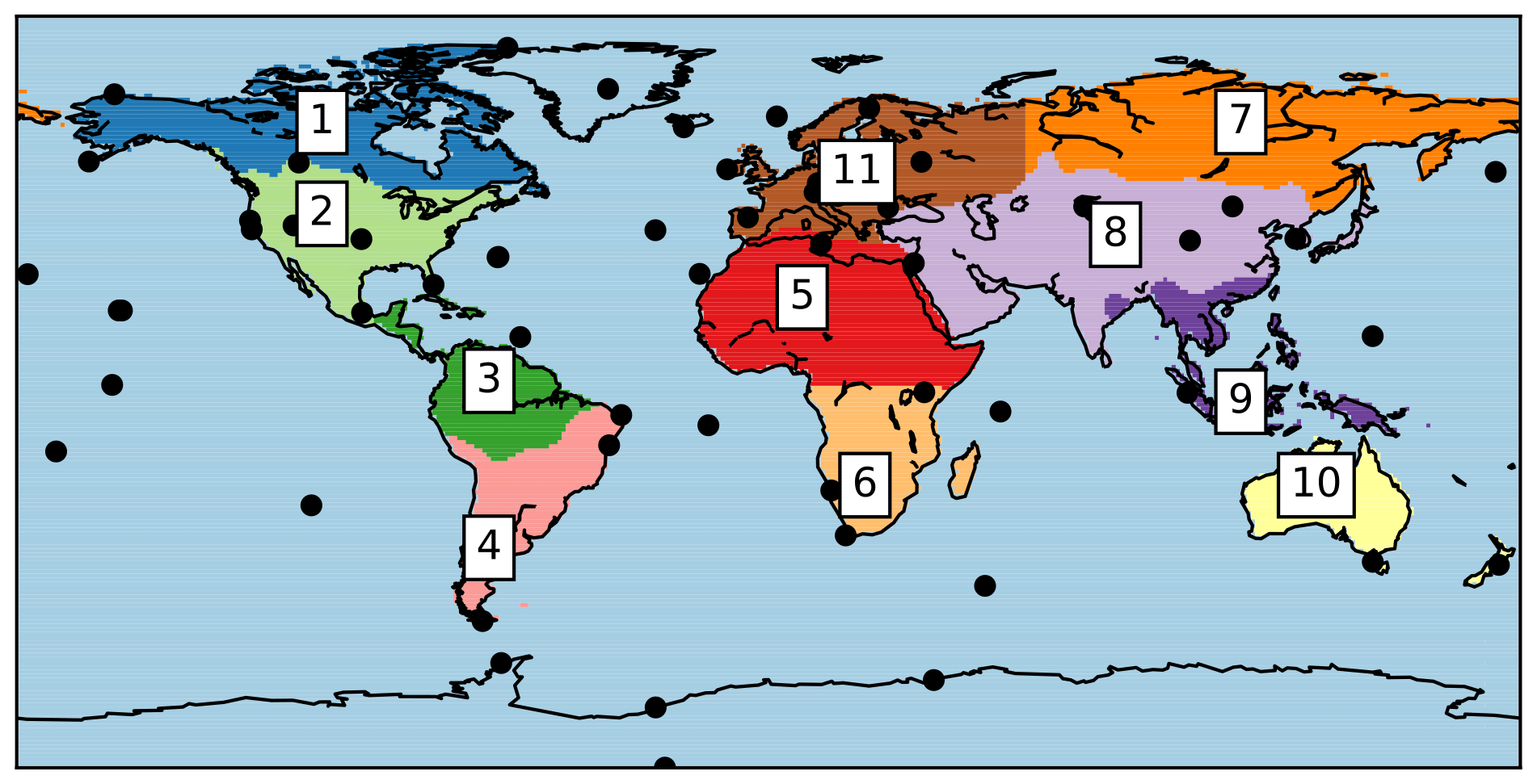
Figure 1 Locations of Global Atmosphere Watch stations, denoted by black dots, and different TransCom regions (different numbers denote the different TransCom regions in this study), denoted by different colours.

2.5 The satellite retrievals

GOSAT (Greenhouse Gases Observing Satellite) from Japan Aerospace Exploration Agency (JAXA) was launched in 2009 and observes column XCO₂ with the TANSO-FTS instrument (Kuze et al., 2009). These data were used to evaluate the different simulations and to assess model performance at larger spatial scales. XCO₂ from the TM5 simulation was calculated using global 4^∘ × 6^∘ × 25 (latitude × longitude × vertical levels) daily average three-dimensional atmospheric CO₂ fields. For each satellite retrieval, the global, three-dimensional, daily mean, gridded atmospheric CO₂ estimates were horizontally interpolated to the location of the retrievals to create the vertical profile of simulated CO₂. Averaging kernels (AKs) (Rodgers and Connor, 2003) were applied to model estimates to ensure a reliable comparison with GOSAT retrievals:

$$\begin{array}{}\text{(6)}& \widehat{C}=c_a+(\mathit{h}\circ \mathit{a}{)}^T(\mathit{x}-{\mathit{x}}_a),\end{array}$$

where $\widehat{C}$ is XCO₂, scalar c_a is the prior XCO₂ of each retrieval, h is a vertical summation vector, a is an absorber-weighted AK of each retrieval, x is a model profile and x_a is the prior profile of the retrieval (Yoshida et al., 2013). The retrievals for different terrestrial TransCom (TC) regions (Fig. 1) were compared with those calculated from the two model simulations. For the comparison with GOSAT XCO₂, the estimates of three-dimensional fields at 6^∘ × 4^∘ resolution were used but not those from the zoom grids due to technical reasons. Differences in XCO₂ due to model resolution were not significant within the context of this study. In this work, GOSAT observations (National Institute for Environmental Studies retrieval V02.21 and V02.31) between July 2009 and the end of 2014 were used.

2.6 Global datasets for evaluating simulated soil carbon and gross primary productivity

For the evaluation of the JSBACH model results, we additionally used data from two soil carbon databases and the FLUXCOM project (Jung et al., 2019). We used the gross primary production (GPP) produced by FLUXCOM, in which eddy covariance flux observations are upscaled using machine learning methods and meteorological and remote sensing data. The FLUXCOM GPP has a 0.5^∘ spatial resolution and 8 d temporal resolution for 2001–2014. Additionally, we used two different soil carbon datasets: SoilGrids (Hengl et al., 2014) and one based on the Harmonised World Soil Database (HWSD) (Batjes, 2016). For the soil carbon data, we used the preprocessed datasets from Fan et al. (2020) that provide values for organic soil carbon down to 1 m depth.

3 Results

3.1 Global carbon fluxes and stocks with the two model formulations

3.1.1 Carbon fluxes

Since the two different model formulations differ only in their soil carbon module formulation, the incoming flux to the ecosystem from photosynthesis is the same in both cases. We analysed results for 2000–2014, and we show here averaged values for that period. The main target variable of our analysis is the heterotrophic respiration, but, to better elucidate how it influences the atmospheric CO₂, we also show net primary production (NPP) and net ecosystem exchange (NEE). NPP is obtained from the gross primary production (GPP) by subtracting autotrophic respiration. NEE is obtained by subtracting from GPP the total ecosystem respiration, direct land cover change, and fire, harvest and herbivory fluxes, as shown in Table 2.

Even though annual total global values of heterotrophic respiration are close between the different model formulations (Table 2), their global seasonal cycles are different (Fig. 2c). The YAS version has a 66 % larger variation of R_h during the year than CBA. Both model versions have their minimum value of R_h in February. While CBA has a maximum in August, YAS reaches its maximum value 1 month earlier, and global R_h also stays high during August. YAS clearly has a steeper increase and decline in its seasonal cycle than CBA. The higher peak of heterotrophic respiration by the YAS model leads to higher global NEE values during June and July (Fig. 2e). In the first 4 months of the year, NEE is higher in the simulations of the CBA model, which is caused by the higher heterotrophic respiration values at this time (Fig. 2e). Autotrophic respiration (which, as explained above, like GPP and NPP is the same for both model formulations) has its highest values in July and August (Fig. S2a). During 2000–2014, both CBA and YAS predict increases in heterotrophic respiration, but only YAS has a significantly increasing trend (p value < 0.005) (Fig. 2). CBA has a larger standard deviation in the annual values (0.87 Pg C) than YAS (0.73 Pg C). The annual NEE time series do not have significant trends, and CBA has larger interannual variability (standard deviation of 0.84 Pg C vs. 0.79 Pg C by YAS).

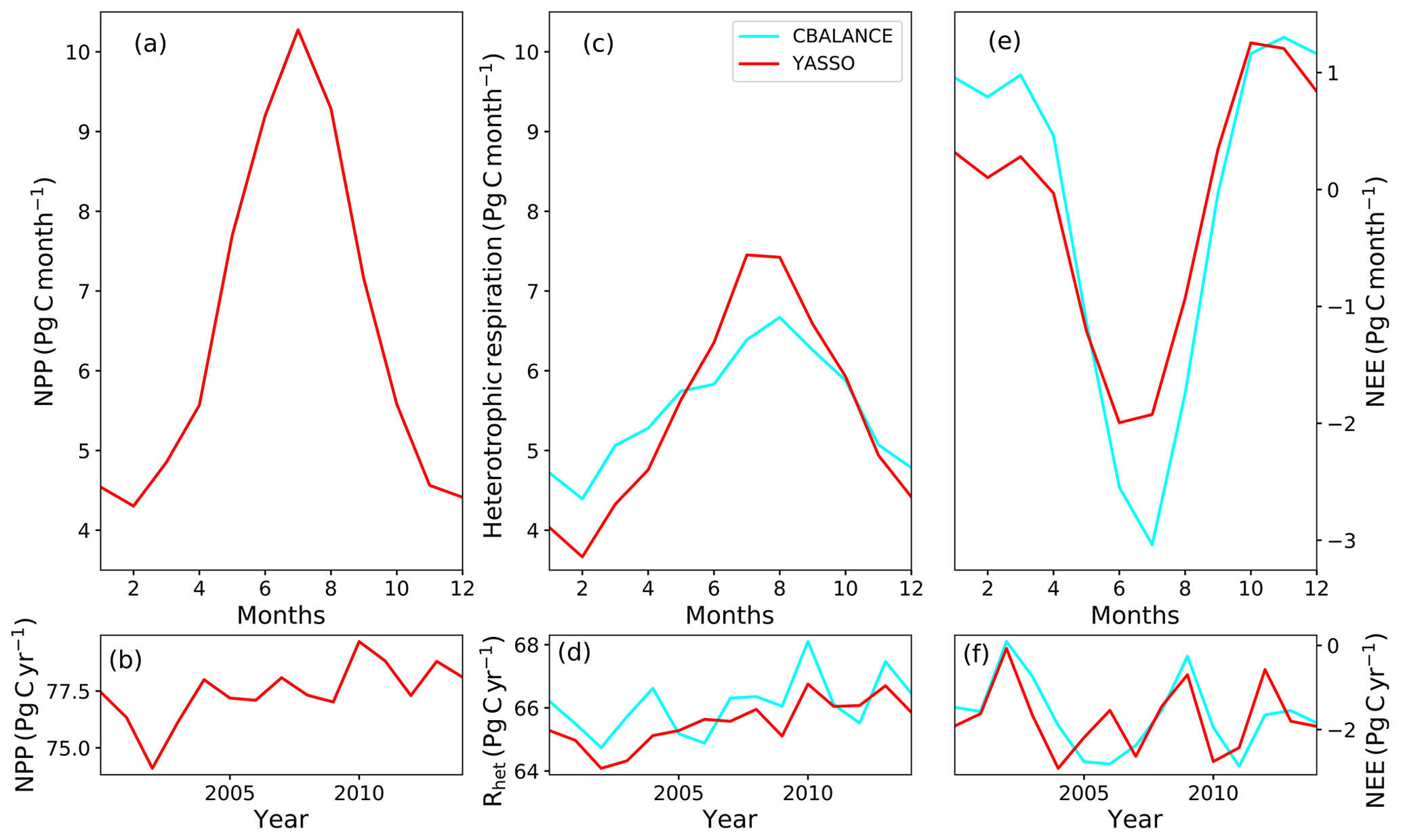
Figure 2 The annual cycles of net primary production (NPP) (a), heterotrophic respiration (c) and net ecosystem exchange (NEE) (e) globally from the CBALANCE (in cyan) and Yasso (in red) model versions. In the sub-panels, annual values are plotted for 2000–2014 for NPP (b), heterotrophic respiration (d) and NEE (f).

In addition to the comparison of the global results, we investigated how the two soil modules differed for broad latitudinally separated regions. The NPP is the same in the different latitudinal regions (Fig. 3a, b). The global total magnitudes of R_h are comparable, while the seasonal cycles show clear differences that are also visible in different latitudinal regions (Fig. 3c, d). The YAS model shows, however, a larger amplitude in the seasonal cycle in all of the regions. In the two most northern regions of the Northern Hemisphere, the amplitude in R_h of YAS is approximately twice the amplitude than that of CBA. In both of these regions, YAS has clear maximum values of R_h in July and August, while the seasonal cycles of CBA are more shallow and do not include such clear maximums. The seasonal cycle of R_h is quite different between the model formulations in the tropics. At 0–30^∘ N, YAS has a seasonal cycle shifted earlier compared to CBA. In this region, YAS has a 42 % larger seasonal amplitude for R_h than CBA. In the Southern Hemisphere regions of 0–10 and 10–30^∘ S, CBA predicts higher values of R_h during the first months of the year after which it stays lower until the end of the year, whereas YAS shows a clear lowering between June and September. In the 10–30^∘ S region, YAS has a 54 % larger amplitude in R_h than CBA. The differences in heterotrophic respiration lead to pronounced differences in the NEE within the tropics (Fig. 3e, f).

Figure 3 The annual cycle of net primary production (NPP) (a, b), heterotrophic respiration (c, d) and net ecosystem exchange (e, f) in the Northern Hemisphere and Southern Hemisphere separated into latitudinal zones. CBALANCE (CBA) results are shown as solid lines and the Yasso (YAS) results as dashed lines.

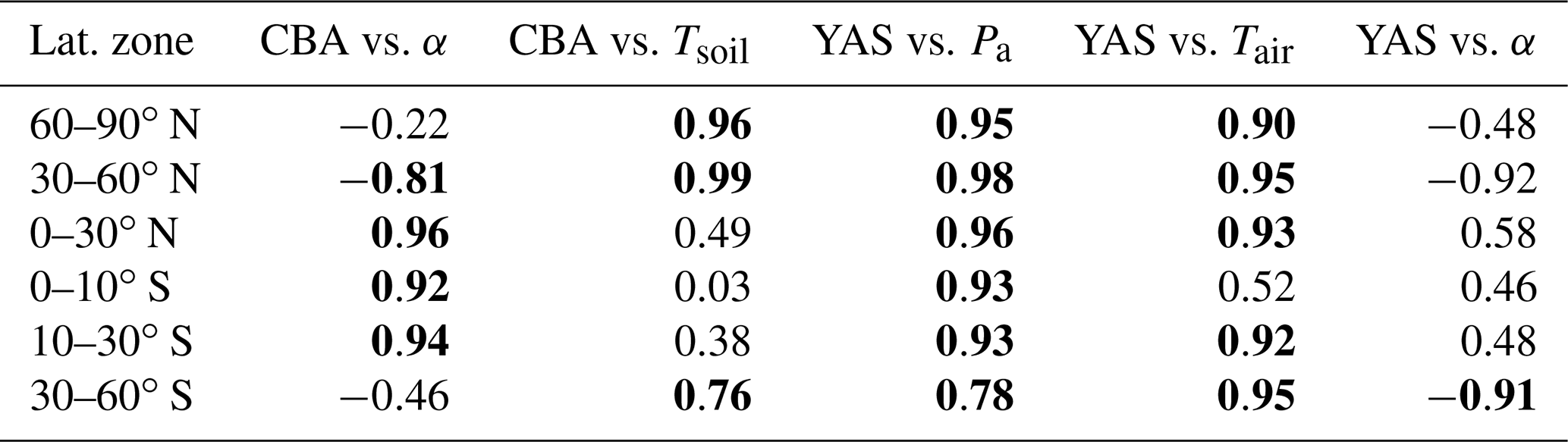
The variation in R_h seasonal dynamics of these two model formulations can be linked to the differences in their environmental drivers and functions. In Table 3, the correlation between heterotrophic respiration and the environmental drivers of each specific model formulation are shown for the different latitudinal regions. Figures S3–S7 in the Supplement show these same relationships. The R_h from CBA has a strong correlation with soil moisture α in the tropical region (30^∘ S–30^∘ N) and a high correlation with soil temperature T_soil at high northern latitudes (30–90^∘ N) and lower, but significant, correlation at high southern latitudes (30–60^∘ S). For other combinations of regions and drivers, the r values are low for CBA, and in three regions, the dependency between α and R_h is negative. In two of these regions with a negative relationship between α and R_h (located at high latitudes), the variability of α is quite small, and the plot shows high scatter (Fig. S3). The shape of the T_soil dependency on the CBA decomposition is exponential, and the relationship is significant when the range of the T_soil values is 15 ^∘C, which is larger than what is occurring in the tropics (Fig. S4).

For the YAS model, on the other hand, R_h shows a strong correlation to its environmental drivers (Table 3). The r values between R_h and precipitation are over 0.90 in all regions except the 30–60^∘ S region. In this region, the correlation is still significant, but the variability of the precipitation is lower than in the other regions (Fig. S5). Therefore, the exponential relationship (Fig. S1d, Eq. 5) between decomposition and precipitation does not lead to a stronger linear relationship in this region. Between air temperature and R_h, the results are similar with the only small r value in the Southern Hemisphere tropics. This region has only a small seasonal variation in air temperature, and the values are also partly located in the temperature range in which the temperature sensitivity of decomposition is weaker (Fig. S6, Eq. 4). The seasonal cycle of R_h predicted by the YAS model does not correlate significantly with the soil moisture variable α in any of these regions (Table 3 and Fig. S7). This is not unexpected as such since α is not the driver of the YAS model. In the tropical region, soil moisture for CBA and precipitation for YAS are more important drivers compared to soil and air temperatures. At high latitudes, temperature has a larger effect on R_h in the results of both models even though in the Northern Hemisphere precipitation also has a significant role for YAS.

We also investigated whether the seasonal cycle of the heterotrophic respiration is correlated with litter fall. The only significant correlation occurred at 30–60^∘ N for both model versions. This was because both have similar annual cycles of R_h and litter fall, but the seasonal cycle of R_h precedes litter fall (Fig. S8).

The global simulated GPP of 167 Pg C yr⁻¹ (Table 2) is highly overestimated when compared to the upscaled data product from FLUXCOM, which gives a mean value of 126 Pg C yr⁻¹ for this time period (Jung et al., 2019) and has a range of 106–130 Pg C yr⁻¹ for a longer time period. Despite the overestimation of global GPP by the model, the comparison to the FLUXCOM product shows that the seasonal cycles in different latitudinal regions are quite similar, although in the northern boreal region, JSBACH reaches maximum GPP values later than the FLUXCOM product (Fig. S9).

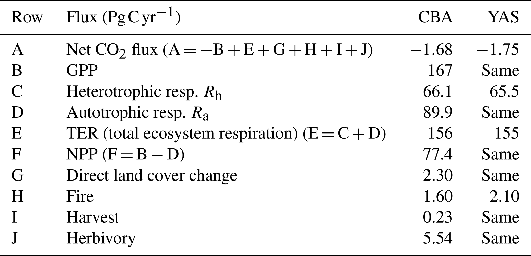
The annual net CO₂ flux shows a slightly larger land sink for YAS than CBA (Table 2). Owing to the larger litter pool, fire fluxes are larger in the YAS model formulation by 0.50 Pg C yr⁻¹; however, they have similar spatial patterns (Fig. S10). This caused the heterotrophic respiration of YAS to be 0.56 Pg C yr⁻¹ smaller than that of CBA since the model was spun up to steady state in 1860 which thus leads to a small discrepancy in net CO₂ fluxes between the two model formulations.

3.1.2 Carbon stocks

The soil carbon stocks simulated by the two models differed in magnitude and also in their latitudinal distributions. The global estimate for total soil carbon by CBA was 4.5-fold larger than that by YAS (Table 1). The global estimate for litter simulated by the YAS model was larger than that simulated by CBA. Vegetation carbon biomass was similar in both model formulations (Table 1).

Table 1 Global C storage in the two different model formulations averaged over 2000–2014. For the YAS model, the eight above-ground pools are summed to obtain the litter pool, while the remaining 10 pools (below ground and humus) represent the soil pool.

The global distribution of soil carbon is very different between the model formulations (Figs. S11c, d, S12). The CBA model has large values of soil carbon at the mid-latitudes of the Northern Hemisphere. YAS predicts larger values in the temperate region of the Northern Hemisphere, but the highest values of soil carbon are located in arctic regions. The data-based estimates from SoilGrids and HWSD also predict the highest values at high northern latitudes (Figs. S11a, b and S12). The CBA model predicts higher values and differing latitudinal patterns south of 60^∘ N compared to the data-based values (Fig. S12). The YAS model shows a very similar behaviour to the HWSD latitudinal pattern and magnitude south of 60^∘ N. The r² and the root mean square errors are generally better for the YAS model than the CBA model when comparing the values along the latitudinal gradient against the data-based products (Table S2).

The turnover times of the two formulations must differ since the soil carbon pools are of very different magnitudes, but the annual R_h between the model formulations is similar. The turnover times, τ, of soil carbon pools can be evaluated at both grid scale and from global values. This global value is obtained by dividing the total soil carbon pool (to which both soil and litter carbon stocks are added) by the annual R_h. Calculated from the global values averaged for 15 years, the apparent turnover time for CBA is 51.3 years and for YAS 14.8 years. The turnover times of CBA are generally longer and show a large spread across different temperatures (Fig. 4a). The YAS model shows a large spread of turnover times at warmer temperatures, but below 0 ^∘C the range is narrower (Fig. 4b). Both models predict the fastest turnover rates in moist and warm conditions. The anomalies of the turnover times are presented in Fig. 5. These have been calculated from the carbon pools over the whole time period and the mean annual R_h. The models show longer turnover times at high northern latitudes and dry areas. The CBA model shows longer turnover times in Central Asia where the moisture conditions limit the decomposition. However, the YAS model does not show such large anomalies in this region.

Figure 4 The turnover times for different temperature and precipitation regimes for the CBALANCE (a) and Yasso (b) models.

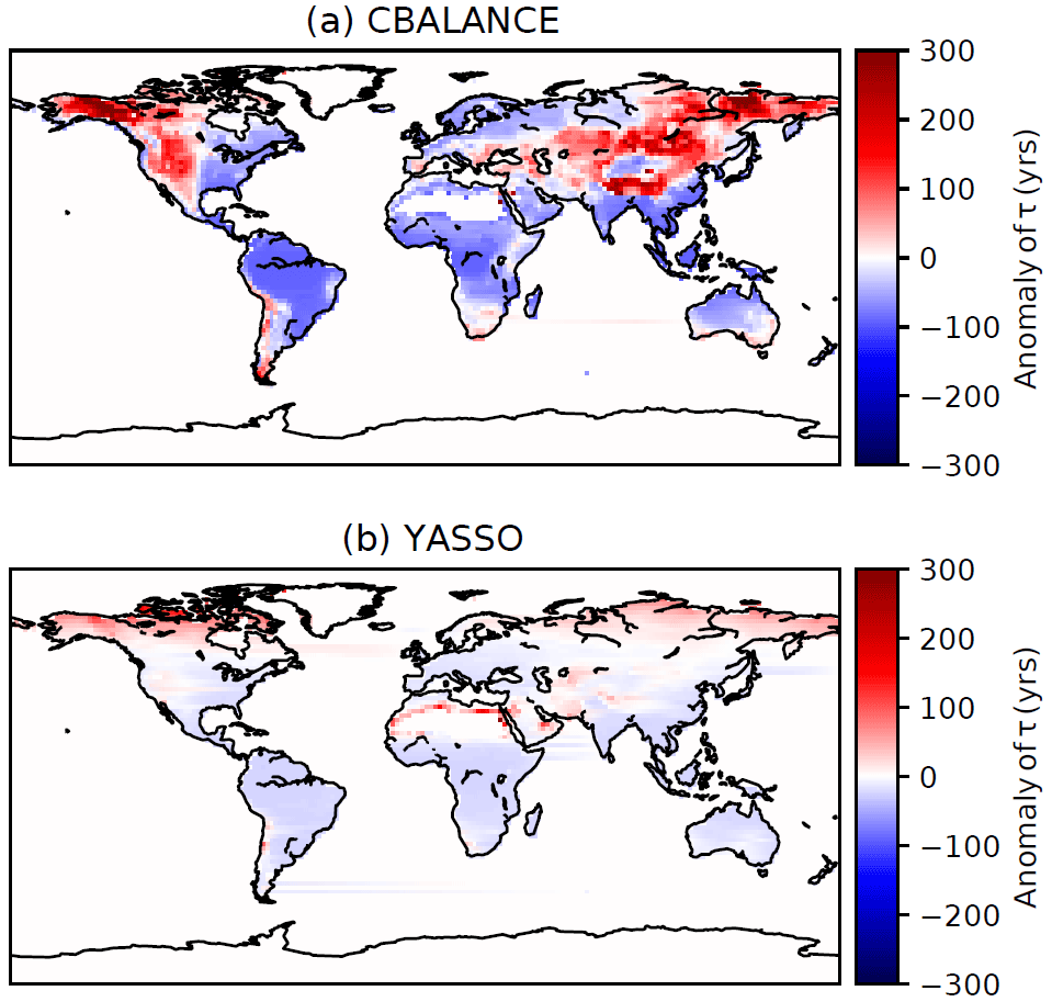
Figure 5 Turnover time, τ, anomalies for CBALANCE (a) and Yasso (b). The average turnover time that was subtracted was 104 years for CBALANCE and 31 years for Yasso.

3.1.3 Box model

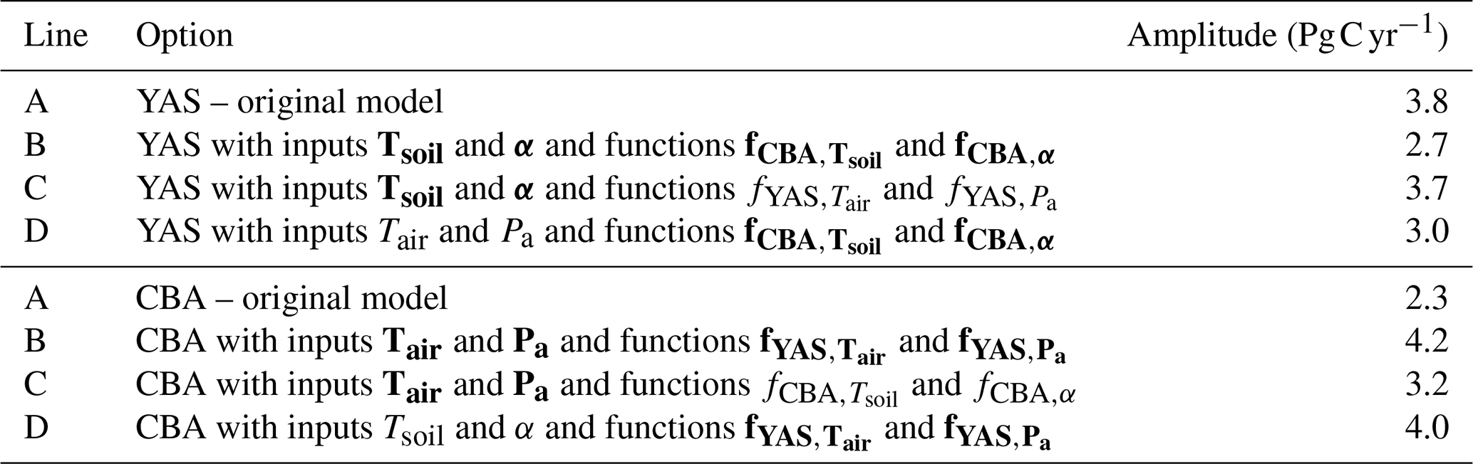
To assess whether the larger seasonal cycle amplitude in R_h by YAS is caused by the larger litter pool or the environmental response functions, a simple box model calculation was performed (detailed description is given in the Appendix). When global respiration was calculated with the turnover times and soil carbon pools of the YAS model but using the environmental responses and drivers of the CBA model, the annual amplitude decreased by 29 % compared to the original YAS model (Table A1). However, the yearly maximum value did not change much. When the opposite was done, and the turnover time and soil carbon pools of CBA were used with the environmental responses and inputs of the YAS model, the magnitude of global heterotrophic respiration increased approximately 1.4-fold (Fig. A1). The increase in the amplitude was 83 % (Table A1). Therefore, this simple analysis suggests that the environmental variables and their response functions cause the larger global amplitude of R_h in the YAS model formulation. To further disentangle whether this change was caused by the different environmental drivers or their functional dependencies, we made additional tests.

The amplitudes of the seasonal cycle of R_h (difference between the maximum and minimum values) are shown in Table A1. For the YAS model, a strong decrease in the amplitude happens when both driver variables and the response functions are changed. When only driver variables are changed, only a slight decrease occurs. When the response functions are changed, the decrease in the amplitude is more pronounced at 21 %. The amplitude predicted by the CBA model increases when the driving variables and response functions are changed (Table A1). This increase occurs when either driving variables or response functions are changed individually. However, with the change in the response functions, the change in amplitude is larger (74 %). In summary, the response functions have a more pronounced role in the changes than the driving variables alone, and this was true for both models.

3.2 Evaluation against surface observations

Seasonal cycle amplitudes of atmospheric CO₂ are successfully simulated by the modelling framework across different latitudes (Fig. 6a). The r² values of the observed seasonal cycle and the model estimates are high across latitudes despite some lower values at mid-latitudes of the Northern Hemisphere (Fig. 6b). Averaged over all latitudes, the r² value, calculated as the linear correlation of simulated and observed averaged annual cycles, was 0.93 for CTE, 0.90 for CBA and 0.87 for YAS.

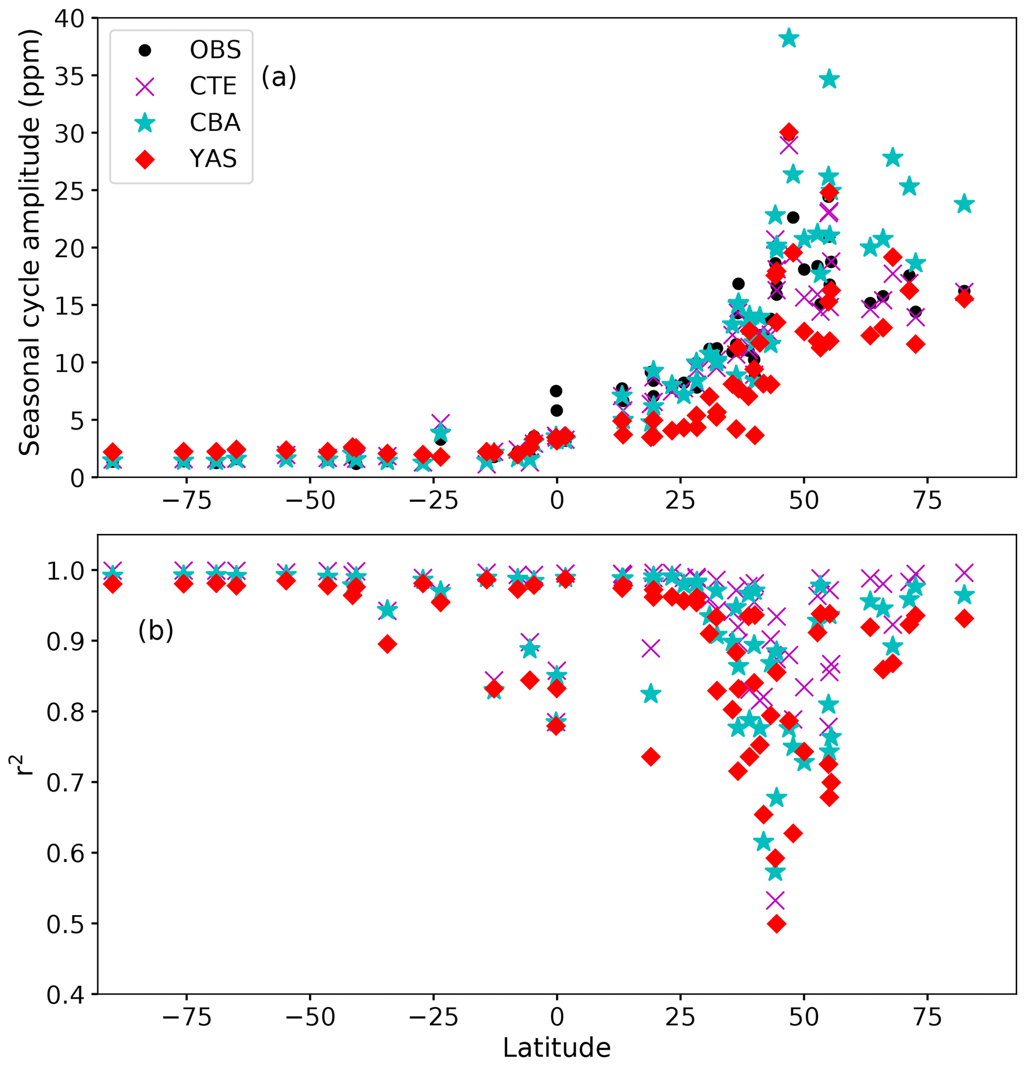
Figure 6 The seasonal cycle amplitudes of atmospheric CO₂ (in ppm) (a) and r² (b) between the simulations and observations at different Global Atmosphere Watch stations as a function of latitude. The black circles denote observations, the magenta crosses are the results from the CarbonTracker Europe 2016 (CTE), the cyan stars are the results from the CBALANCE (CBA) run, and the red diamonds are the results from the Yasso (YAS) run.

The capability of the model formulations to simulate the amplitude of the seasonal cycle differs within latitudinal regions (Fig. 6). The CBA model is able to capture the timing of the seasonal cycle at northern latitudes but has a tendency to overestimate the seasonal cycle amplitude by about 30 % north of 45^∘ N. In this region, the underestimation of seasonal cycle amplitude by CTE is approximately 5 % and by YAS 14 %. In the 0–45^∘ N region, YAS underestimates the seasonal cycle amplitude, on average, by approximately 32 %, whereas CTE underestimates it by 4 % and CBA overestimates it by 1 %. The agreement between estimated atmospheric CO₂ and observations was worse in YAS than in CBA when considering the r² value and the seasonal cycle. Overall, the magnitude of the seasonal cycle amplitude predicted by YAS had less bias north of 45^∘ N compared to CBA but large underestimations at latitudes of 0–45^∘ N where CBA was very successful in simulating the right seasonal cycle amplitude.

Four surface observation sites in the Northern Hemisphere illustrate a similar behaviour in the seasonal cycle and its amplitudes as described above (Fig. 7 and Table S3). To confirm the general quality of the TM5 model used for both YAS and CBA, we plotted its biospheric a posteriori fluxes from CarbonTracker Europe 2016; indeed, deviations between CTE and observations are much smaller than from the JSBACH model at all sites. At the high-latitude sites, Alert and Pallas (Fig. 7a, e), CBA overestimates the seasonal cycle amplitude, while YAS shows some phase shift of the cycle. The observed seasonal cycle amplitudes are smaller at the two more southern sites, Niwot Ridge and Mauna Loa. For those sites, CBA is generally successful in capturing their magnitude (Table S3), whereas YAS underestimates them strongly. YAS also has difficulty capturing the seasonal pattern at Niwot Ridge. This was happening generally in the temperate region, as is also seen in the lower r² values of the YAS model at the different sites (Fig. 6).

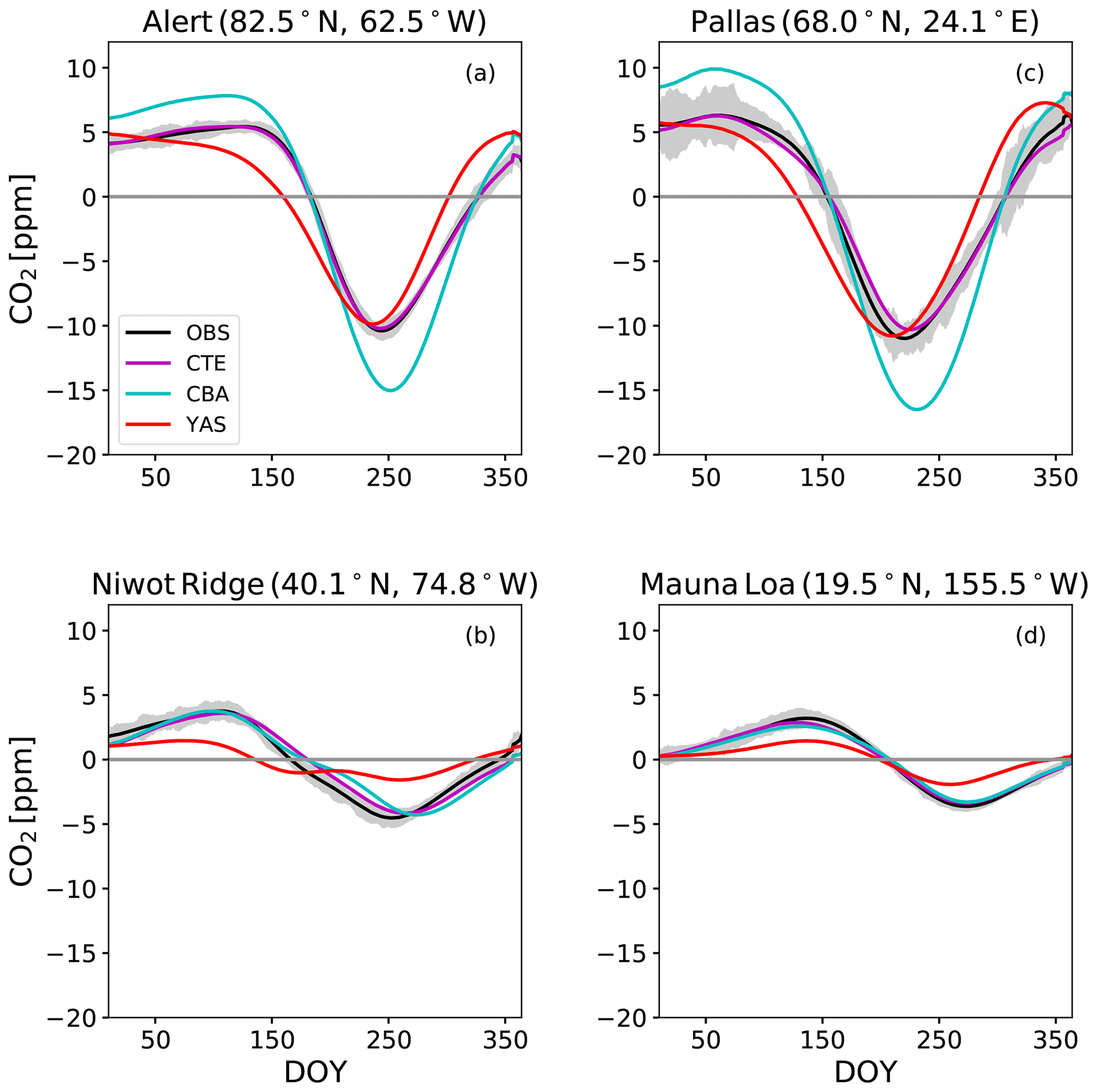
Figure 7 The detrended seasonal cycles of atmospheric CO₂ at four Global Atmospheric Watch sites, Alert (a), Pallas (c), Niwot Ridge (b) and Mauna Loa (d), for observations (OBS) in black, CarbonTracker Europe 2016 (CTE) in magenta and the two JSBACH model versions with CBALANCE (CBA) with the cyan lines and Yasso (YAS) with the red lines. The solid grey line denotes the zero line. The grey shaded area shows the standard deviations of the observations after detrending. DOY denotes day of year.

When comparing the overall bias in atmospheric CO₂ at these four sites between the observations and the model simulations, CBA overestimated CO₂ by 3.65 ppm and YAS by 2.27 ppm when averaged over all the measurements within the study period. A closer look at the bias at Mauna Loa (Fig. S13) revealed biases in the 2000–2014 trends for CBA and YAS, whereas CTE shows no bias in the trends. The CBA overestimates CO₂ by 1.76 ppm in the beginning and by 3.74 ppm in 2014. The overestimates by YAS are smaller: 1.12 ppm in 2000 and 3.14 in 2014. The results at surface sites show that CBA largely overestimated seasonal cycle amplitude at high northern latitudes, whereas YAS almost consistently underestimated the seasonal cycle amplitude in the Northern Hemisphere. CBA captured the seasonal cycle patterns better than YAS across different latitudes. Overall, the YAS model showed biases in the atmospheric CO₂ cycle at temperate latitudes in the Northern Hemisphere, whereas the CBA model had biases at high latitudes in the Northern Hemisphere.

3.3 Column XCO₂ comparisons for TransCom regions

This evaluation of the two soil modules against satellite column XCO₂ was carried out for the different TransCom (TC) regions (Fig. 1). The comparison was based on seasonal cycle amplitudes and r² values similar to the surface site evaluation. Not all the TC regions show a clear seasonal cycle, such as regions in South America (TC regions 3 and 4), the northern part of Africa (TC = 5) and Australia (TC = 10). For completeness, we show the analysis also for these regions in Table S5. For regions with clear seasonal cycles, we used the ccgcrv curve fitting procedure available from NOAA (https://www.esrl.noaa.gov/gmd/ccgg/mbl/crvfit/crvfit.html, last access: 1 July 2017; Thoning et al., 1989), but for regions with missing data or no clear seasonal cycle, we averaged over all years of data.

To further illustrate the results from this comparison, we show data for two regions that have a clear seasonal cycle. In TC region 2, the southern part of North America, CBA is more successful in capturing the observed seasonal cycle amplitude than YAS (Fig. 8a) even though CBA reaches the minimum XCO₂ later than observations. YAS underestimates the seasonal cycle amplitude by 56 % and has a different seasonal pattern than observations, so the minimum is reached earlier than in the observations and also the shape during the summer period differs from the observations. In Europe, TC region 11, both models capture the seasonal cycle amplitude (Fig. 8b, Table S4) and the seasonal cycle in the first part of the year. The increase of CO₂ in autumn is not captured so well by the simulations.

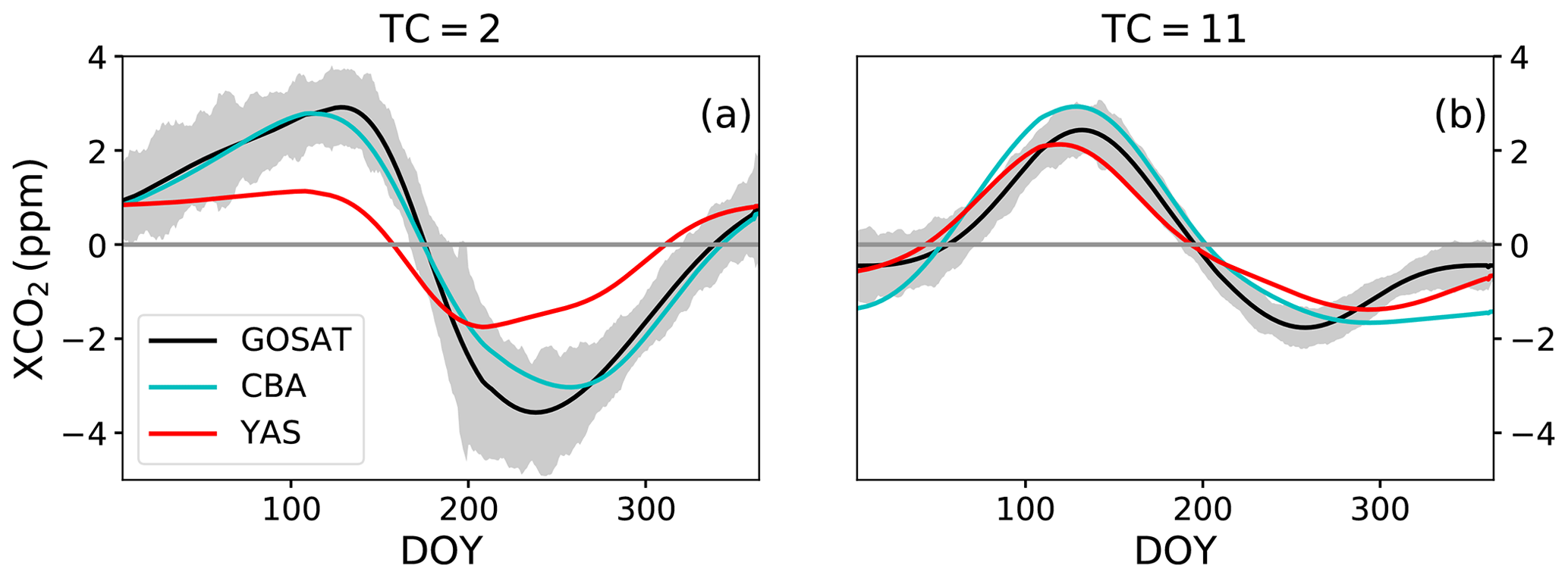
Figure 8 The seasonal cycles of detrended atmospheric XCO₂ at TransCom region 2, the southern part of North America (a), and region 11, Europe (b). The grey line shows the standard deviations of the observations after detrending. The observations are in black, CBALANCE (CBA) model results in cyan and Yasso (YAS) model results in red. The solid grey line denotes the zero line, and DOY denotes day of year.

Overall, observed XCO₂ and simulated XCO₂ differ from each other in ways similar to the surface site observations. Estimates of seasonal cycle amplitude by YAS are too small at mid-latitudes (Fig. 8a) and in TC regions 2, 5 and 8 compared to the observations, and CBA is better at capturing the observed annual cycles. At TC = 1 (the northern part of North America), CBA overestimates the seasonal cycle amplitude, while YAS better captures it. However, the seasonal cycle pattern is better captured with CBA (Table S4) than with YAS. Generally, YAS had smaller seasonal cycle amplitudes than the observations, and CBA was more consistent with the observations in most TC regions. CBA is also better than YAS in capturing the seasonal pattern of XCO₂ in all TC regions (Table S4).

There is bias in absolute XCO₂ between the GOSAT retrievals and the model simulations. When averaged over the time period used and the TC regions, CBA overestimates the GOSAT observations by 3.37 ppm and YAS by 2.33 ppm. These values were in line with the bias in absolute CO₂ estimates at the four surface sites.

4 Discussion

In this work, our aim was to use atmospheric observations to assess whether soil carbon models of a land surface model can be evaluated with this kind of framework. Our main finding was that the two models predicted different annual cycles of global R_h with the YAS model having a larger amplitude. This, in turn, leads to clear differences in the model predictions of seasonal cycles of the atmospheric CO₂ concentration at surface stations and TC regions. To attribute the differences between the two models to a specific cause, we need to compare their results from their different aspects and to also judge whether our model simulations are reasonable in light of previous research.

4.1 Evaluation of carbon fluxes

Annual heterotrophic respiration was 66.1 Pg C yr⁻¹ for CBA and 65.5 Pg C yr⁻¹ for YAS (Table 2), which fall into the range of estimates from Earth system models (41.3–71.6 Pg C yr⁻¹) and are close to the observation-based estimate of 60 Pg C yr⁻¹ (Shao et al., 2013). Part of the difference between CBA and YAS is caused by the fire fluxes. The YAS model has a larger litter pool that behaves as fuel for fires. Therefore, to have the system at steady state, global heterotrophic respiration by YAS must be less. Moreover, the simulation time of 140 years before the beginning of the analysis might cause some divergence between the model runs.

Table 2 Global terrestrial C fluxes from the two different model formulations averaged over 2001–2014.

Moving to monthly timescales, we can see that the global seasonal R_h cycle had a larger amplitude with YAS than with CBA (Fig. 2), and a simple box model calculation found that environmental drivers and their response functions are the cause, not the large litter pool in the YAS model. It is anyhow challenging to further disentangle whether this larger amplitude is mainly caused by the differing environmental drivers of the soil carbon models or the functional dependencies of those drivers play a bigger role. The analysis by the box model suggested a stronger role of the response functions compared to the driving variables at monthly timescales, but strong conclusions cannot be drawn from such a simple analysis. Other studies have also shown that the response functions themselves lead to pronounced differences between soil carbon models (Wieder et al., 2018).

When heterotrophic respiration is compared by latitudinal zones, differences between the model formulations are visible in the variability and timing of the seasonal cycles in many regions (Fig. 3). R_h correlates strongly with the environmental drivers of the models in different latitudinal zones (Table 3). Both models are largely influenced by their moisture dependency in the tropical region (Table 3). CBA is driven by soil moisture in a linear dependence, and YAS is driven by precipitation in an exponential relationship. Since the ranges of precipitation are larger than the variability in soil moisture and due to the exponential relationship between precipitation and decomposition in YAS, YAS is more tightly coupled with moisture than CBA. At annual timescales, for which the YAS model was originally developed, precipitation and soil moisture behave similarly. However, the seasonal cycles of the two variables are different. Precipitation begins earlier in the season in the tropical region, and it causes YAS to reach yearly maximum heterotrophic respiration earlier than CBA, which is driven by soil moisture in this region. Likewise, air and soil temperatures are more similar in the long term than in the short term. Particularly in the temperate region, where the temperature plays a larger role, the air temperature has larger variability than soil temperature, and this leads to a different kind of seasonal pattern of the R_h predictions by the two different soil models.

Table 3 The Pearson correlation r values for the different latitudinal zones between modelled heterotrophic respiration and the environmental drivers of the CBALANCE (CBA) and Yasso (YAS) models. The environmental drivers are all calculated as monthly means for the latitudinal zones. Significant correlation (p value < 0.05) have been written in bold; α is the relative soil moisture, T_soil and T_air are soil and air temperature, and P_a is the precipitation.

The observations show that litterfall has strong influences on heterotrophic respiration (Chemidlin Prévost-Bouré et al., 2010). At seasonal timescales in the different latitudinal zones, there is no clear influence of litterfall driving the heterotrophic respiration seen in the models, which primarily results from the pre-defined turnover times of the fast litter pools smoothing out individual litter fall events. Changes in the chemical composition of litterfall are considered to be one potential reason for changes in the amplitude of atmospheric CO₂ (Randerson et al., 1997), and this is something we could study with the YAS model.

Different moisture dependencies of R_h have previously been found to be important (Exbrayat et al., 2013). At the global level, Hursh et al. (2017) recommended using parabolic soil moisture functions in preference of functions based on mean annual precipitation. Their study considered soil respiration; i.e. the autotrophic respiration of roots was also included. Ťupek et al. (2019) evaluated the YAS model against R_h observations at two coniferous sites in southern Finland and found problems in capturing the seasonality in the observations and the variability in the summertime fluxes. One reason they mention for this is the response of the simulated R_h to soil moisture conditions since R_h is not attenuated in very moist conditions, and they found a need to improve the moisture dependency of the YAS model. This is in line with our findings in that a model that has been parameterised at annual timescales requires further development before it can be reliably applied at shorter timescales. Precipitation was originally used in the YAS model as a proxy for soil moisture since enough accurate soil moisture observations for model development were not available. Clearly, this idea needs to be reconsidered as our results show that at zonal spatial scales and monthly temporal scales, R_h from YAS is not correlated with the soil moisture.

Simulated global GPP (165 Pg C yr⁻¹) is notably larger than the estimated 106–130 Pg C yr⁻¹ derived from FLUXCOM for the time period. However, the simulated value is still within the range of other data-driven estimates such as the one from the Carbon Cycle Data Assimilation system being 146 (± 19) Pg C yr⁻¹ (for 1980–1999) (Koffi et al., 2012) and isotope-based estimates being 150 to 175 Pg C yr⁻¹ (for 1980–2009) (Welp et al., 2011). Figure S9 shows that the bias relative to FLUXCOM exists throughout most of the Northern Hemisphere and the tropics but has only a minor influence on the seasonal cycle of GPP. The high estimate of GPP will propagate into larger NPP, litter input, and therefore also simulated heterotrophic respiration and soil carbon stocks. While this may contribute to a slightly larger simulated seasonal cycle of atmospheric CO₂ at northern stations, it is unlikely that this will affect our conclusions on the impact of the different soil formulations on the ability of JSBACH to simulate the seasonal cycle of heterotrophic respiration, the residence time of carbon in soil and, as a consequence, its ability to reproduce the observed seasonal cycle of atmospheric CO₂ or its long-term trend. Nevertheless, this comparison shows that in order to further improve JSBACH's performance against these data, GPP biases should be reduced. Furthermore, the high GPP values resulting from the simulations would likely be lower if the nutrient cycles of nitrogen and phosphorus were included in the version of JSBACH used (Goll et al., 2012). Beside using a JSBACH version with nutrient cycles, further development work on the phenological cycle could improve the estimated GPP. The difference of the modelled GPP to the FLUXCOM product (Fig. S9) suggests that the maximum leaf area index might be overestimated in the tropics. Also, the timing of the phenological cycle north of 60^∘ N might benefit from re-parameterisation.

4.2 Evaluation of carbon stocks and turnover times

The two soil models predicted different global soil carbon stocks (Table 1) with different latitudinal distributions (Fig. S12). Similar to earlier studies (Goll et al., 2015; Thum et al., 2011), in our results the YAS model was more successful than CBA in estimating global soil carbon stocks that are similar to estimates from observations, approximately 1500 Pg C including large uncertainties (from 504 to 3000 Pg C) (Scharlemann et al., 2014), as can be seen in the different estimates from HWSD (1578 Pg C) and SoilGrids (2870 Pg C) (see also Tifafi et al., 2018). The YAS model is widely used in different applications at smaller scales, and its performance to estimate soil carbon stocks has been found to be good (Hernández et al., 2017). Comparability between the model-calculated and the observed carbon stocks is relevant for any analyses of carbon fluxes because in both models investigated here, the fluxes are proportional to the stocks (flux equals decomposition rate times stock). Modelled global vegetation carbon was within the observation-based estimate of 442±146 Pg C of Carvalhais et al. (2014).

The distribution of soil carbon stocks was also more realistic in YAS than in CBA (Fig. S12, Table S2). The large soil carbon stocks at mid-latitudes predicted by CBA (Figs. S11c, S12) are unrealistic compared to current data-based estimates of the global soil carbon distribution (Fig. S12). The large carbon stocks at high latitudes predicted by the YAS model (Figs. S11d, S12) are more in line with the observations but miss the high values observed from peatlands and permafrost in high-latitude regions. The version of JSBACH used does not include peatlands and is modelling only mineral soils. Therefore, the large carbon reservoirs of peatlands are not captured by the model. This JSBACH version also did not have permafrost described. If permafrost would be modelled, the seasonal cycle of heterotrophic respiration at high latitudes would likely be dampened as the depth of the active layer determines the amount of soil capable of respiring. The YAS model has been used in a JSBACH version containing permafrost in a study concentrating on the Russian far east (Castro-Morales et al., 2018). Both CBA and YAS were originally developed for mineral soils and for applications with organic soil, so model development and testing at smaller than global scales could be useful.

The environmental responses of the turnover times have quite different forms for the two soil carbon models (Fig. 4). The CBA model shows a wide distribution of turnover times across the whole temperature range, whereas the YAS model shows a larger spread in the tropical temperature range. This large spread in warm conditions is also observed (Koven et al., 2017) and is caused by the saturating temperature function of the YAS model, as shown in Fig. S1c. The large spread in turnover times as predicted by the CBA model might be caused by the fact that CBA is driven by soil temperature in one soil layer. The environmental responses of the turnover times at annual timescales behave in a similar way as those at monthly timescales so that moisture is a more important driver in warm regions and temperature in cold regions, as was seen in Table 3.

The study by Koven et al. (2017) provided an empirically based turnover time as a function of temperature. At 20 ^∘C, this turnover time was approximately 11±2 years, which is closer to the estimate of the YAS model (calculated for values of 19.5–20.5^∘C and their standard deviation) being 22±21 years and much lower compared to the CBA estimate of 64±37 years. At lower temperatures, at −15 ^∘C, the empirically based turnover time is 200±100 years, and YAS underestimates this with 82±41 years (calculated for values $-\mathrm{15.5}-(-\mathrm{14.5})$ ^∘C), whereas the prediction by CBA is closer (150±80 years). Therefore, the turnover times simulated with the YAS model are closer to the observations in warm temperatures, but the turnover times are too low in cold temperatures. CBA estimated turnover times that are too high in warm temperatures, but turnover times in colder temperatures were in the same order of the observations.

The global turnover time of soil carbon by CBA was somewhat larger than in an earlier study, where it was estimated to be 40.8 years (Todd-Brown et al., 2014). This value was at the higher end of the CMIP5 models. The global turnover time from YAS, which was 14.8 years, is more in the range of the other CMIP5 models (Todd-Brown et al., 2014). The spatial distribution of the turnover time anomalies shows differences caused by the environmental drivers and their dependencies at annual timescales. When comparing these overall turnover times of total soil carbon, it is important to keep in mind that both models consisted of carbon pools that had widely varying turnover times. For example, despite the higher overall turnover time, the turnover time of the most recalcitrant carbon pool of YAS was an order of magnitude smaller than that of CBA.

4.3 Evaluation using atmospheric CO₂

The differences between the two models in the seasonal cycle of atmospheric CO₂ were strong. CBA better reproduced the seasonal cycle amplitudes, capturing the shape of the seasonal cycle both for surface sites and comparisons in the TC regions even though its soil carbon distribution had a worse performance compared to YAS. CBA exaggerated the seasonal cycle amplitudes at high northern latitudes, as was found previously (Dalmonech and Zaehle, 2013). It is important to keep in mind that this study was done within a land surface model and that modelled GPP was biased. The simulated GPP had a larger magnitude and some bias in its seasonal cycle, and therefore its evaluation against atmospheric CO₂ observations is influenced by it. Even though the atmospheric observations provide a valuable and informative comparison for the model results, their use as a benchmark metric needs careful consideration.

The differences in absolute CO₂ and XCO₂ levels against the surface observations and the satellite retrievals, respectively, with modelled CO₂ are caused by the modelling system, but this bias does not influence the analysis performed. We obtained the land surface fluxes (GPP, respiration, fire and herbivory fluxes and land-use change emissions) from JSBACH and, together with the rest of the fluxes from CarbonTracker Europe2016 (CTE), we used TM5 to obtain atmospheric CO₂ values. Fossil fuel emissions have not been optimised in CTE. Therefore, we obtained ocean fluxes that had been optimised with the land carbon cycle of CTE and that differ from the JSBACH estimate. The land carbon cycle of CTE is modelled by the SiBCASA-GFED4 model (van der Velde et al., 2014) and fire emissions that were estimated from satellite-observed burned areas (Giglio et al., 2013). The net global a posteriori land sink of CTE is approximately $-\mathrm{2.0}(\pm \mathrm{1.1})$ Pg C yr⁻¹ for 2001–2014. On the other hand, the JSBACH estimate for the net land sink is approximately −1.7 Pg C yr⁻¹ (Table 2) and is therefore smaller than the land sink of CTE. The fire flux of JSBACH is modelled, whereas the estimate of CTE is based on data. As shown in Fig. S13 for Mauna Loa, the bias in the CO₂ develops during the study period, and the plot shows consistency so that YAS, which predicts a net land sink closer to CTE than CBA, has a smaller bias at the end of the time period. We concentrated the analysis on the averaged seasonal cycles that are not influenced by this linear increase.

The space-borne observations give a similar message as the surface observations in TransCom regions, which showed a clear seasonal cycle. Niwot Ridge is located in TransCom region 2 (southern part of North America); there YAS also showed an amplitude that was too low, and CBA performed better, in a similar way as seen in the Fig. 8. The Pallas site is located in TransCom region 11 (Europe), and at Pallas the seasonal cycle was more pronounced than in Europe as a whole, but, similar to the surface observations at Pallas and TransCom region 11, the models both perform acceptably. Using large TransCom regions helped us to interpret the signal despite the larger variability than in the surface observations (comparing grey shaded regions in Figs. 7 and 8), and it has been recommended to use the information content of the satellites at continental scales (Miller et al., 2018).

The transport model itself also brings uncertainty to the result. The modelling of atmospheric transport is a challenging task as open scientific questions in the field remain (Crotwell and Steinbacher, 2018), and the models contain biases (Gurney et al., 2004). The errors in atmospheric transport models cause a substantial difference in the inverse CO₂ model flux estimates (Peylin et al., 2013). However, in this study we only used one atmospheric transport model. It is expected that the biases, as only one transport model was used, are similar between the two soil model runs and are not the cause for the large differences seen in the two simulations.

5 Conclusions

We demonstrated how atmospheric CO₂ observations can be used to evaluate two soil carbon models within the same land surface model and the different viewpoints offered by several variables considered. We used two different soil carbon models within one land surface model and used a three-dimensional transport model to obtain atmospheric CO₂ while obtaining the anthropogenic and ocean fluxes from CarbonTracker Europe framework. We evaluated the carbon stocks of the soil models and compared seasonal cycles calculated with soil carbon fluxes from the soil models to atmospheric CO₂ results from both surface and space-born observations. This work highlighted how the changes in the heterotrophic respiration transfer to the net ecosystem exchange estimates and further to the atmospheric CO₂ signal. We also discussed the importance of the model drivers and their functional dependencies, which differed for the two soil carbon models we studied. When considering both surface- and space-based observations, it is not straightforward to say which of the two soil carbon models performed better.

The comparison of the two soil carbon models revealed large differences in their estimates. The YAS model better captured the magnitude and spatial distribution of soil carbon stocks globally. However, it was biased in its atmospheric CO₂ cycle at temperate latitudes in the Northern Hemisphere. The CBA model, on the other hand, showed better performance in capturing the seasonal cycle pattern of atmospheric CO₂, but it is biased at high latitudes in the Northern Hemisphere. R_h from the YAS model showed a misalignment with soil water content in tropical regions as they were negatively correlated with each other. This suggests that the use of precipitation as a proxy for soil moisture might not be sensible at sub-annual timescales and calls for improvement in the parameterisation of the YAS model. The use of this modelling system can help us to assess the global consequences of the new YAS parameterisation if this were done. The drivers of YAS have larger variability in their values during the seasonal cycle that causes a more pronounced seasonal cycle in the heterotrophic respiration with the current parameterisation. Concerning the results, this leads to unrealistic seasonal cycles of CO₂ in temperate regions and the tropics and calls for model improvement. CBA showed less pronounced seasonal cycles of heterotrophic respiration and had issues with CO₂ amplitude only at high northern latitudes. The linear moisture dependence therefore seems justified; however, it likely causes the Central Asian region to have carbon stocks that are too large. Whether this is caused by drought sensitivity that is too high or problems in the predicted soil moisture by JSBACH is difficult to judge. The amplitude that is too high in the high northern regions might be a result of the biases in the gross fluxes of the modelling system.

The evaluation was done within a land surface model that overestimates GPP in comparison to an upscaled GPP product, and this hampers doing benchmarking using this modelling system. Since the model is run to a steady state during the spin-up procedure, it also leads to other biases in the modelling system (influencing, for example, autotrophic respiration). Overestimated GPP leads to an enhanced litter input to the soil. This causes the comparison of the magnitudes of the soil carbon pools to the actual observations to be cumbersome as the overestimated litter fall causes biases in the model estimates. In this study, the magnitudes of simulated soil carbon are therefore not as good as the spatial patterns as an indicator of the model performance (such as latitudinal gradient). The other downside of the GPP biases is their influence on the estimated NEE. Due to the biases in the timing and magnitude of the other carbon fluxes, it is challenging to use CO₂ as a benchmark for heterotrophic respiration. However, in our study, the two soil models lead to pronounced differences in the atmospheric CO₂, and we were also able to locate latitudinal regions where the models had the most issues. Therefore, this approach provides a method to evaluate how the changes in the heterotrophic fluxes further influence the atmospheric signal and helps us to track which geographical areas are contributing to the questionable model performance.

Soil carbon models have several development needs (Bradford et al., 2016; van Groenigen et al., 2017) that are now partly being answered with next generation models which include more mechanistic representation of several below-ground processes (Wieder et al., 2015; Yu et al., 2020). The development of moisture dependency from simple empirical relationships is moving towards mechanistic approaches which may yield more reliable results in the long term (Yan et al., 2018). Our results confirm that the moisture dependency of heterotrophic respiration plays on important role in the whole global carbon cycle.

In this study, we used space-born XCO₂ observations in addition to the surface observations of CO₂. They were providing a larger-scale confirmation of the results obtained from the surface observations and thus provided complementary information. The number of satellite observations of column XCO₂ are increasing at a fast pace; for example, Orbiting Carbon Observatory-2 (OCO-2) observations started in 2014, and they hold great potential for carbon cycle studies (Miller and Michalak, 2020).

Appendix A: Description of the box model

A simple box model calculation was performed to evaluate the importance of the dependencies of environmental drivers and the soil carbon pool sizes on the larger global seasonal cycle amplitude in R_h as predicted by YAS. In this box model, we assume that heterotrophic respiration R_h is a product of environmental dependencies and the turnover time as follows:

$$\begin{array}{}\text{(A1)}& \begin{array}{rl}& R_{\mathrm{h},\mathrm{YAS}}=b\cdot f_{\mathrm{YAS},T_{\mathrm{air}}}\left(T_{\mathrm{air}}\right)\cdot f_{\mathrm{YAS},P_{\mathrm{a}}}\left(P_{\mathrm{a}}\right)\cdot {\displaystyle \frac{C_{\mathrm{soil},\mathrm{YAS}}}{{\mathit{\tau }}_{\mathrm{YAS}}}},\\ & \mathrm{where}b={\displaystyle \frac{\mathrm{\Sigma }{f}_{\mathrm{CBA},T_{\mathrm{soil}}}\left(T_{\mathrm{soil}}\right)\cdot f_{\mathrm{CBA},\mathit{\alpha }}\left(\mathit{\alpha }\right)}{\mathrm{\Sigma }{f}_{\mathrm{YAS},T_{\mathrm{air}}}\left(T_{\mathrm{air}}\right)\cdot f_{\mathrm{YAS},P_{\mathrm{a}}}\left(P_{\mathrm{a}}\right)}},\end{array}\end{array}$$

where R_h,YAS is the heterotrophic respiration of model YAS, b is a scalar that takes into account the different magnitudes of the response functions, T_air is air temperature, P_a is annual precipitation, C_soil,YAS is the total soil carbon pools, and τ_YAS is the turnover time of the total soil carbon pools. T_soil is soil temperature, and α is the relative soil moisture. This formulation in Eq. (A1) refers to the YAS model. The response functions are as shown in Sect. 2.1.2. For the CBA model, the formulation is as follows:

$$\begin{array}{}\text{(A2)}& R_{\mathrm{h},\mathrm{CBA}}={\displaystyle \frac{\mathrm{1}}{b}}\cdot f_{\mathrm{CBA},T_{\mathrm{soil}}}\left(T_{\mathrm{soil}}\right)\cdot f_{\mathrm{CBA},\mathit{\alpha }}\left(\mathit{\alpha }\right)\cdot {\displaystyle \frac{C_{\mathrm{soil},\mathrm{CBA}}}{{\mathit{\tau }}_{\mathrm{CBA}}}}.\end{array}$$

These responses were introduced in Sect. 2.1.1.

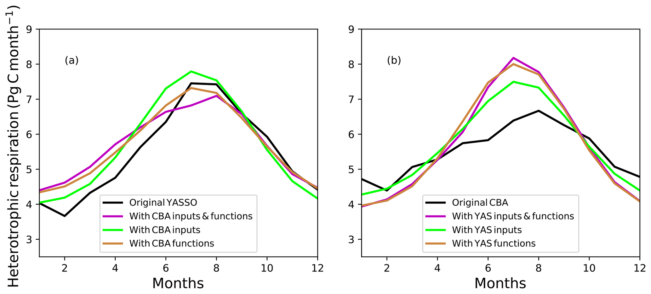
Figure A1 Different annual cycles of the heterotrophic respiration (R_h) predicted by the Yasso (YAS) (a) and CBALANCE (CBA) (b) model and the different alternatives from the box model calculation.

The equations used monthly heterotrophic respiration, environmental drivers and soil carbon stocks averaged over 2000–2014 to estimate the turnover times for each grid point for YAS using Eq. (A1) and for CBA using Eq. (A2). Using these turnover times, we calculated global R_h with the turnover times and soil carbon pools of each model by making different tests. First, we used the environmental responses and drivers of the other model (lines B in Table A1). Additionally, we changed the driving variables but kept the original response functions (lines C in Table A1). Then we changed only the response functions of the original model while keeping the original driving variables (lines D in Table A1).

Since the driving variables of soil moisture and annual precipitation differed in magnitude by approximately 4-fold, soil moisture was multiplied by 4 when using the function for annual precipitation ($f_{\mathrm{YAS},P_{\mathrm{a}}}$), and when annual precipitation was used in the function for soil moisture (f_CBA,α), it was divided by 4. The annual cycles of R_h are shown in Fig. A1 and the amplitudes in Table A1.

Table A1 The amplitude of global heterotrophic respiration within a year in different box model formulations. The input variables or functions that differ from the original model formulation are in bold letters.