the Creative Commons Attribution 4.0 License.
the Creative Commons Attribution 4.0 License.
 | 23 Nov 2020
A numerical model study of the main factors contributing to hypoxia and its interannual and short-term variability in the East China Sea
Haiyan Zhang
Arnaud Laurent
Changwei Bian
A three-dimensional physical-biological model of the marginal seas of China was used to analyze interannual and intra-seasonal variations in hypoxic conditions and identify the main processes controlling their generation off the Changjiang (or Yangtze River) estuary. The model was compared against available observations and reproduces the observed temporal and spatial variability of physical and biological properties including bottom oxygen. Interannual variations of hypoxic extent in the simulation are partly explained by variations in river discharge but not nutrient load. As riverine inputs of freshwater and nutrients are consistently high, promoting large productivity and subsequent oxygen consumption in the region affected by the river plume, wind forcing is important in modulating interannual and short-term variability. Wind direction is relevant because it determines the spatial extent and distribution of the freshwater plume, which is strongly affected by either upwelling or downwelling conditions. High-wind events can lead to partial reoxygenation of bottom waters and, when occurring in succession throughout the hypoxic season, can effectively suppress the development of hypoxic conditions, thus influencing interannual variability. A model-derived oxygen budget is presented and suggests that sediment oxygen consumption is the dominant oxygen sink below the pycnocline and that advection of oxygen in the bottom waters acts as an oxygen sink in spring but becomes a source during hypoxic conditions in summer, especially in the southern part of the hypoxic region, which is influenced by open-ocean intrusions.
- Article
(7180 KB) - Full-text XML
- Companion paper
-
Supplement
(5128 KB) - BibTeX
- EndNote


In coastal seas, hypoxic conditions (oxygen concentrations lower than 2 mg L−1 or 62.5 mmol m−3) are increasingly caused by rising anthropogenic nutrient loads from land (Diaz and Rosenberg, 2008; Rabalais et al., 2010; Fennel and Testa, 2019). Hypoxic conditions are detrimental to coastal ecosystems, leading to a decrease in species diversity and rendering these systems less resilient (Baird et al., 2004; Bishop et al., 2006; Wu, 2002). Hypoxia is especially prevalent in coastal systems influenced by major rivers such as the northern Gulf of Mexico (Bianchi et al., 2010), Chesapeake Bay (Li et al., 2016), and the Changjiang (or Yangtze River) estuary (CE) in the East China Sea (ECS; Li et al., 2002).
The Changjiang is the largest river in China and fifth largest in the world in terms of volume transport, with an annual discharge of 9 × 10¹¹ m3 yr−1 via its estuary (Liu et al., 2003). The mouth of the CE is at the confluence of the southeastward Yellow Sea Coastal Current and the northward Taiwan Warm Current (Fig. 1). Hydrographic properties in the outflow region of the CE are influenced by several different water masses, including fresh Changjiang Diluted Water, relatively low-salinity coastal water; more saline water from the Taiwan Warm Current; and high-nutrient, low-oxygen water from the subsurface of the Kuroshio Current (Qian et al., 2017; Wei et al., 2015; Yuan et al., 2008). The interactions of these water masses together with wind forcing and tidal effects lead to a complicated and dynamic environment.
Freshwater (FW) discharge by the Changjiang reaches its minimum in winter when the strong northerly monsoon (dry season) prevails and peaks in summer during the weak southerly monsoon (wet season), resulting in a large FW plume adjacent to the estuary. Along with the FW, the Changjiang delivers large quantities of nutrients to the ECS, resulting in eutrophication in the plume region (Li et al., 2014; Wang et al., 2016). Since the 1970s, nutrient load has increased more than 2-fold, with a subsequent increase in primary production (PP) in the outflow region of the estuary (Liu et al., 2015). Hypoxia off the CE was first detected in 1959 and, with a spatial extent of up to 15 000 km2, is among the largest coastal hypoxic zones in the world (Fennel and Testa, 2019). Although no conclusive trend in oxygen minima has been observed (Wang, 2009; Zhu et al., 2011), hypoxic conditions are suspected to have expanded and intensified in recent decades (Li et al., 2011; Ning et al., 2011) due to the increasing nutrient loads from the Changjiang (Liu et al., 2015).
It is generally accepted that water-column stratification and the decomposition of organic matter are the two essential factors for hypoxia generation, and this is also the case for the shelf region off the CE (Chen et al., 2007; Li et al., 2002; Wei et al., 2007). High solar radiation and FW input in summer contribute to strong vertical stratification, which is further enhanced by near-bottom advection of waters with high salinities (> 34) and low temperatures (< 19 ∘C) by the Taiwan Warm Current. The resulting strong stratification inhibits vertical oxygen supply (Li et al., 2002; Wang, 2009; Wei et al., 2007). At the same time, a large supply of organic matter fuels microbial oxygen consumption (OC) in the subsurface (Li et al., 2002; Wang, 2009; Wei et al., 2007; Zhu et al., 2011). It has also been suggested that the Taiwan Warm Current brings additional nutrients contributing to organic matter production (Ning et al., 2011) and that the low oxygen concentrations (∼ 5 mg L−1) of the Taiwan Warm Current precondition the region to hypoxia (Ning et al., 2011; Wang, 2009).
While observational analyses suggest that hypoxia off the CE results from the interaction of various physical and biogeochemical processes, quantifying the relative importance of these processes and revealing the dynamic mechanisms underlying hypoxia development and variability require numerical modeling (Peña et al., 2010). Numerical modeling studies have proven useful for many other coastal hypoxic regions such as the Black Sea northwestern shelf (Capet et al., 2013), Chesapeake Bay (Li et al., 2016; Scully, 2013), and the northern Gulf of Mexico (Fennel et al., 2013; Laurent and Fennel, 2014). Models have also been used to study the hypoxic region of the CE. Chen et al. (2015a) used a 3D circulation model with a highly simplified oxygen consumption parameterization (a constant consumption rate) to investigate the effects of physical processes – i.e., FW discharge and wind speed and direction – on the dissipation of hypoxia. Chen et al. (2015b) examined the tidal modulation of hypoxia. The model domain in these two previous studies was relatively limited – encompassing only the CE, Hangzhou Bay, and the adjacent coastal ocean – and did not cover the whole area affected by hypoxia (Wang, 2009; Zhu et al., 2011). Zheng et al. (2016) employed a nitrogen cycle model coupled with a 3D hydrodynamic model to examine the role of river discharge and wind speed and direction on hypoxia, and also emphasized the physical controls. These previous modeling studies focused on the response of hypoxia to physical factors only and did not address seasonal evolution and interannual variations of hypoxia or the influence of variability in biological rates.
More recently, Zhou et al. (2017) analyzed the seasonal evolution of hypoxia and the importance of the Taiwan Warm Current and Kuroshio Current intrusions as a nutrient source using an advanced coupled hydrodynamic-biological model. However, the baseline of their model does not include sediment oxygen consumption (SOC), which is thought to be a major oxygen sink in the hypoxic region off the CE (Zhang et al., 2017) and other river-dominated hypoxic regions, including the northern Gulf of Mexico (Fennel et al., 2013; Yu et al., 2015a, b). Zhou et al. (2017) acknowledged the importance of SOC based on results from a sensitivity experiment but did not quantify its role in hypoxia generation.
Here we introduce a new 3D physical-biological model implementation for the ECS that explicitly includes nitrogen and phosphorus cycling and SOC. The model is a new regional implementation for the ECS of an existing physical-biogeochemical model framework that has been extensively used and validated for the northern Gulf of Mexico (Fennel et al., 2011, 2013; Laurent et al., 2012; Laurent and Fennel, 2014; Yu et al., 2015b; Fennel and Laurent, 2018). The hypoxic zones in the northern Gulf of Mexico and off the CE have similar features, including the dominant influence of a major river (Changjiang and Mississippi), a seasonal recurrence every summer, a typical maximum size of about 15 000 km2, documented phosphorus limitation following the major annual discharge in spring, and a significant contribution of SOC to oxygen sinks in the hypoxic zone (Fennel and Testa, 2019).
We performed and assessed a 6-year simulation of the ECS and use the model results here to identify the main factors driving hypoxia variability on interannual and short-term (days to seasons) timescales in the simulation. More specifically, we investigate the role of interannual variations in riverine inputs of nutrients and FW versus short-term variations in coastal circulation and mixing. We also present an oxygen budget to quantify the relative importance of SOC and the influence of lateral advection of oxygen in the model. The companion study by Grosse et al. (2020) used the same model to quantify the importance of intrusions of nutrient-rich oceanic water from the Kuroshio Current for hypoxia development off the CE.
2.1 Physical model
The physical model is based on the Regional Ocean Modeling System (ROMS; Haidvogel et al., 2008) and was implemented for the ECS by Bian et al. (2013a). The model domain extends from 20 to 42∘ N and 116 to 134∘ E (Fig. 1), covering the Bohai Sea, the Yellow Sea (YS), the ECS, part of the Sea of Japan, and the adjacent western North Pacific, with a horizontal resolution of 1∕12∘ (about 10 km) and 30 vertical layers with enhanced resolution near the surface and bottom. The model uses the recursive Multidimensional Positive Definite Advection Transport Algorithm (MPDATA) for the advection of tracers (Smolarkiewicz and Margolin, 1998), a third-order upstream advection of momentum, and the generic length scale (GLS) turbulence closure scheme (Umlauf and Burchard, 2003) for vertical mixing.
The model is initialized with climatological temperature and salinity from the World Ocean Atlas 2013 (WOA13) (Locarnini et al., 2013; Zweng et al., 2013) and is forced by 6-hourly wind stress, and heat and FW fluxes from the ECMWF ERA-Interim data set (Dee et al., 2011). Open boundary conditions for temperature and salinity are also from WOA13, and horizontal velocities and sea surface elevation at the boundaries are specified from the monthly SODA data set (Carton and Giese, 2008). In addition, eight tidal constituents (M2, S2, N2, K2, K1, O1, P1, and Q1) are imposed based on tidal elevations and currents extracted from the global inverse tide model TPXO7.2 of Oregon State University (Egbert and Erofeeva, 2002). At the open boundaries, Chapman and Flather conditions are used for free surface and barotropic velocities, respectively, and the radiation condition for the baroclinic velocity. Eleven rivers are included in the model. FW discharge from the Changjiang uses daily observations from Datong Hydrological Station. For the other rivers, we prescribed monthly or annual climatologies (Liu et al., 2009; Tong et al., 2015; Zhang, 1996).
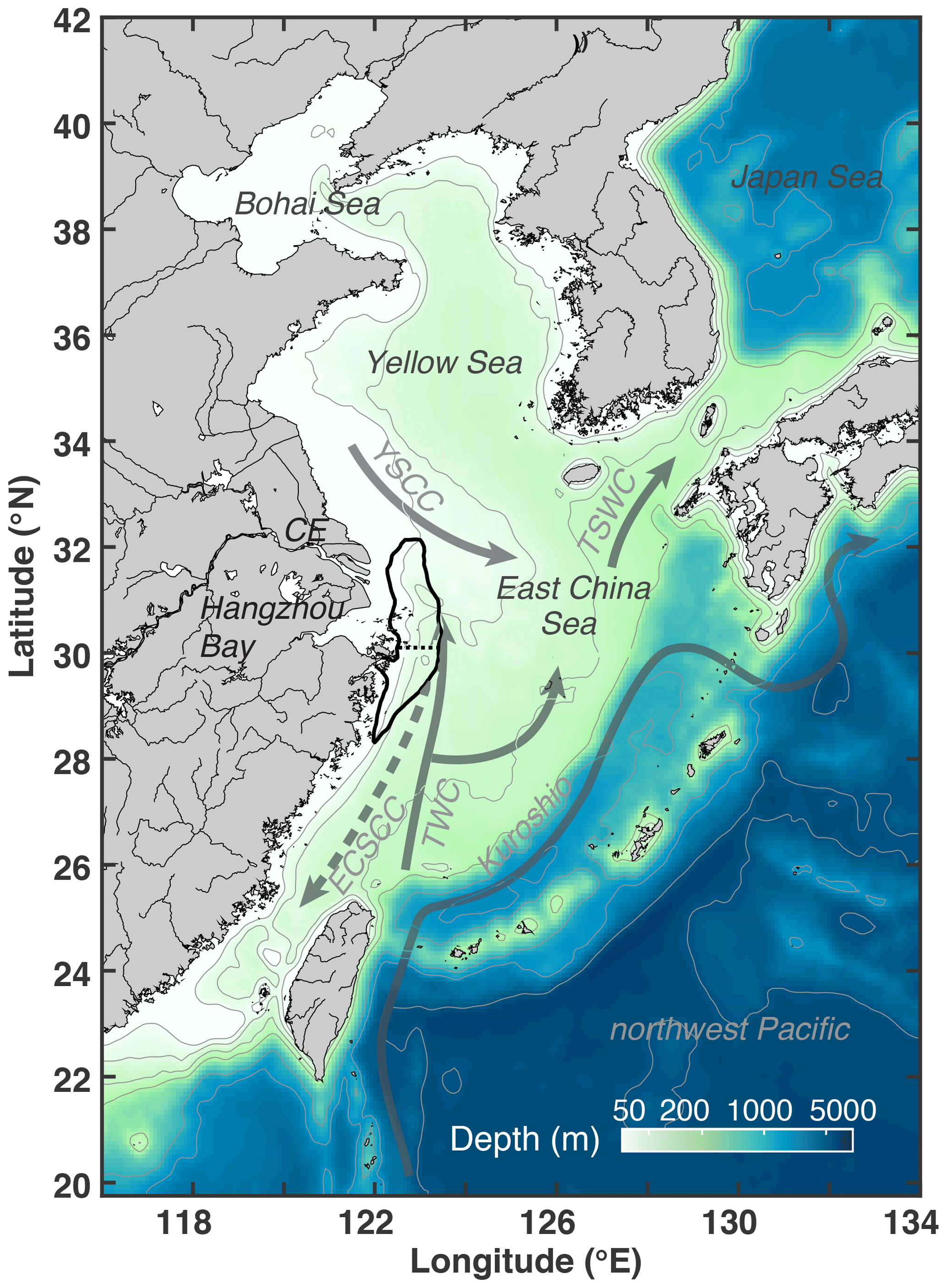
Figure 1Bathymetry of the model domain with 30, 50, 100, 200, 1000, 2000, and 5000 m isobaths. The black outline near the Changjiang Estuary (CE) and Hangzhou Bay indicates the zone typically affected by low-oxygen conditions (dotted line shows separation between northern and southern zones). Solid grey arrows denote currents present throughout the year (Kuroshio; TWC: Taiwan Warm Current; YSCC: Yellow Sea Coastal Current; TSWC: Tsushima Warm Current). The dashed grey arrow indicates the direction of the wintertime East China Sea Coastal Current (ECSCC), which flows in the opposite direction in summer.
2.2 Biological model
The biological component is based on the pelagic nitrogen cycle model of Fennel et al. (2006, 2011, 2013) and was extended to include phosphate (Laurent et al., 2012; Laurent and Fennel, 2014) and riverine dissolved organic matter (Yu et al., 2015b). The model includes two forms of dissolved inorganic nitrogen (DIN), nitrate (NO3) and ammonium (NH4); phosphate (PO4); phytoplankton (Phy); chlorophyll (Chl); zooplankton (Zoo); two pools of detritus, suspended and slow-sinking small detritus (SDet) and fast-sinking large detritus (LDet); and riverine dissolved organic matter (RDOM). Here, riverine dissolved and particulate organic nitrogen enter the pools of RDOM and SDet, respectively. The remineralization rate of RDOM is an order of magnitude lower than that of SDet to account for the more refractory nature of the riverine dissolved organic matter (Yu et al., 2015b).
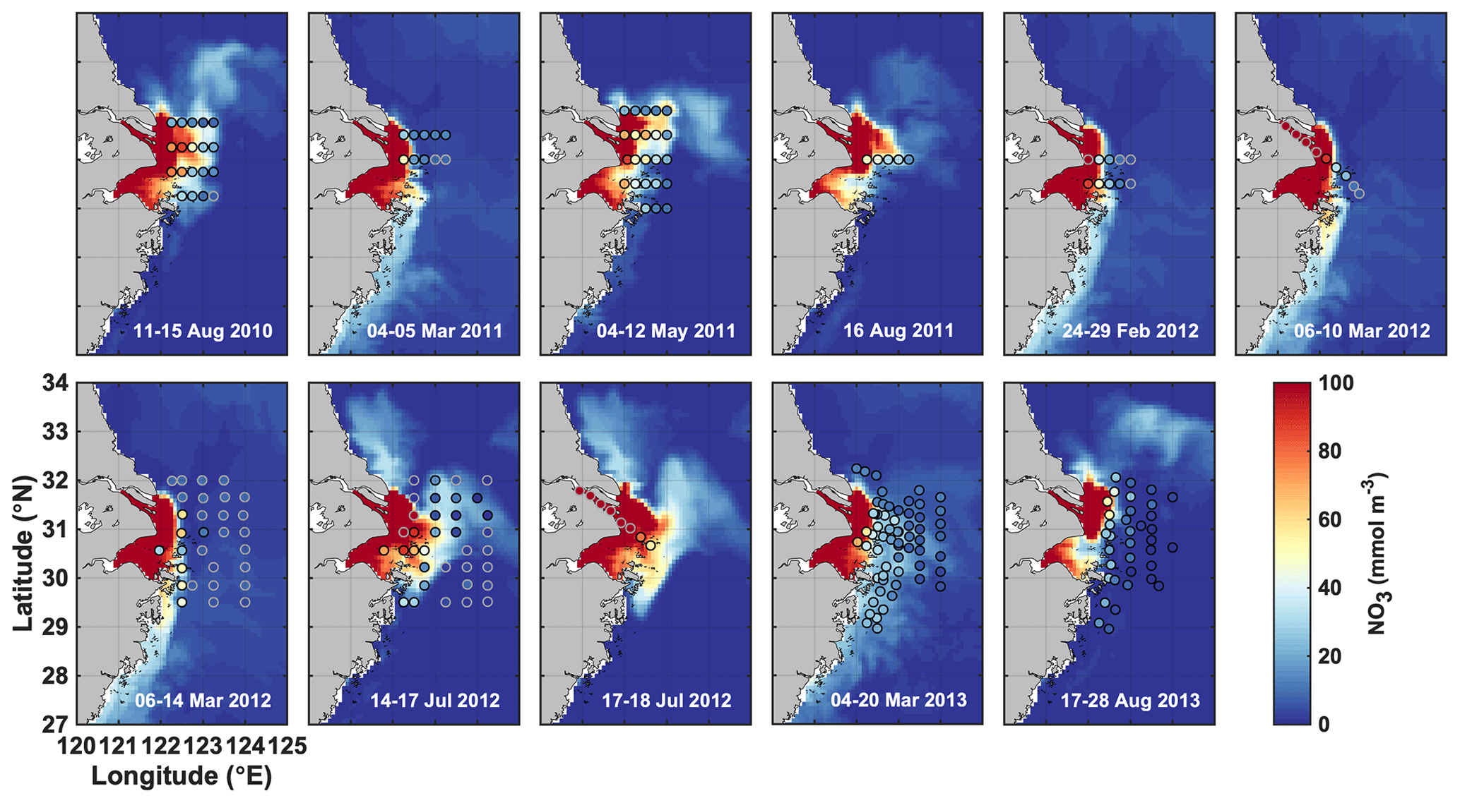
Figure 2Simulated surface nitrate (colored map) shown for the day that marks the mid-point of the cruise dates (given in each panel) compared to observations (dots) during 11 cruises from 2011 to 2013.
At the sediment–water interface, SOC is parameterized assuming “instantaneous remineralization”; i.e., all organic matter reaching the sediment is remineralized instantaneously, and oxygen is consumed due to nitrification and aerobic remineralization at the same time. In the instantaneous remineralization, all phosphorus is returned to the water column as PO4, while a constant fraction of fixed nitrogen is lost due to denitrification. All biogeochemical model parameters are given in Table S1 in the Supplement. More detailed model descriptions can be found in the Supplement to Laurent et al. (2017). Light is vertically attenuated by chlorophyll, detritus, and seawater itself. In addition, to account for the effects of colored dissolved organic matter (CDOM) and suspended sediments, which show relatively high values near the coast and in the river plume (Bian et al., 2013b; Chen et al., 2014), a light-attenuation term dependent on water depth and salinity is introduced which yields higher attenuation in shallow areas and in the FW plume.
Initial and boundary conditions for NO3, PO4, and oxygen are prescribed using WOA13 (Garcia et al., 2013a, b). A small positive value is used for the other variables. NO3 is nudged towards climatology in the western North Pacific at depth > 200 m. Monthly nutrient loads of NO3 and PO4 from the Changjiang are from the Global NEWs model (Wang et al., 2015) but were adjusted by multiplicative factors of 1.20 and 1.66, respectively, to ensure a match between simulated and observed nutrient concentrations in the CE (see July and August 2012 in Fig. 2). Nutrient loads in other rivers are based on other published climatologies (Liu et al., 2009; Tong et al., 2015; Zhang, 1996). Due to a lack of data on organic matter loads, river load concentrations of SDet, LDet, and RDOM were assumed conservatively at 0.5, 0.2, and 15 mmol N m−3, respectively.
We performed an 8-year simulation from 1 January 2006 to 31 December 2013, with 2006–2007 as model spin-up and 2008–2013 used for analysis. Model output was saved daily.
3.1 Model validation
Model output is compared with observations of simulated surface and bottom temperature, salinity, current patterns and strength, surface chlorophyll, surface nitrate, and bottom oxygen. The model reproduces remotely sensed spatial and temporal sea surface temperature (SST) patterns very well (Fig. S1), with an overall correlation coefficient – i.e., considering all climatological monthly mean SST fields interpolated to the model grid – of 0.98. Simulated surface and bottom salinity also show similar spatial and seasonal patterns as available in situ observations (Figs. S2 and S3) with overall correlation coefficients – i.e., using all surface and all bottom data points – of 0.77 and 0.84, respectively. Simulated surface and bottom temperature, when compared with available in situ data (Figs. S4 and S5), are also consistent with the observations, with overall correlation coefficients of 0.96 and 0.93.

Figure 3Simulated bottom oxygen (colored map) shown for the day that marks the mid-point of the cruise dates compared with observations (dots) during nine cruises from 2011 to 2013.
The simulated current systems in the ECS and YS show typical seasonal variations as follows (see also Fig. S6). In winter, currents mainly flow southward on the Yellow Sea and ECS shelves driven by the northerly wind. In contrast, the ECS Coastal Current and the Korean Coastal Current flow northward in summer. The Kuroshio Current is stronger in summer than in winter. The model captures the seasonal pattern of the current system and resolves currents in the ECS and Yellow Sea (also see Grosse et al., 2020).
Simulated monthly averaged (2008–2013) surface chlorophyll concentrations in May, August, and November are compared with satellite-derived fields and agree well with spatial correlation coefficients of 0.77, 0.94, and 0.64, respectively (Fig. S7).
Simulated surface nitrate concentrations are shown in comparison to in situ observations in Fig. 2 and agree well with an overall correlation coefficient of 0.84. Observations in March and July of 2012 show strongly elevated concentrations in the CE and a sharp gradient in the vicinity of the estuary's mouth that are well represented by the model. Likewise, simulated and observed bottom oxygen distributions are compared in Fig. 3 and agree reasonably well overall with an overall correlation coefficient of 0.71, although the model underestimates observed low-oxygen conditions in July of 2011 and 2013 and August 2013.
Together, these comparisons show that the model is able to reproduce important aspects of the physical-biogeochemical dynamics in the study region.
3.2 Simulated oxygen dynamics
First, we describe the timing and distribution of simulated bottom-water oxygen off the CE to set the stage for our investigation into the drivers underlying hypoxia variability. The model simulates annually recurring hypoxic conditions with a typical seasonal cycle where bottom waters are well oxygenated until April/May, and hypoxic conditions are established in June or July, become more pronounced in August, and disperse in October or November (Fig. 4a, c). However, the model also simulates significant interannual variability in timing and extent of hypoxia over the 6-year simulation period (Fig. 4b, c). The years with largest maximum hypoxic extent are 2010 (20 520 km2), 2009 (16 660 km2), 2012 (13 930 km2), and 2008 (12 720 km2), while the simulated hypoxic extent is much smaller (< 5000 km2) in 2011 and 2013. The ranking is similar when considering the time-integrated hypoxic extent (Fig. 4b). The year with the largest maximum and integrated hypoxic extent (2010) also has the highest peak discharge (Fig. 4a) and highest annual FW discharge (65 400 m3 s−1), although the annual discharge in 2008 and 2012 is not much smaller than in 2010.
The region where low-oxygen conditions are most commonly simulated is indicated by the frequency map in Fig. 4d, which shows the total number of days in the 6-year simulation when bottom oxygen concentrations were below 125 mmol m−3 (or 4 mg L−1), i.e., twice the hypoxic threshold. It is known from observations that there are two centers of recurring hypoxic conditions: the northern core is located just to the east of the CE and Hangzhou Bay, and the southern core to the southeast of Hangzhou Bay. The model is consistent with these observations and simulates two distinct core regions of low-oxygen conditions centered at 31 and 29.3∘ N. The northern core region is larger than the southern core region (9050 km2 for a threshold of 80 d per year of < 4 mg L−1 compared to 5230 km2). We will refer to the region defined by a threshold of 40 d of < 4 mg L−1 of per year (solid black line in Figs. 1 and 4d) as the “typical low-oxygen zone” for the remainder of the paper and demarcate the northern and southern sections by 30.1∘ N latitude (dashed line in Figs. 1 and 4d).
There are marked differences in the phenology of simulated hypoxic extent (Fig. 4c). Among the 4 years with largest hypoxic areas, hypoxia is established relatively late (mid-August), and lasts long (into November) in 2008 and 2009. In contrast in 2012, hypoxic conditions are established earlier (June), are most pronounced in August and are eroded by mid-October. In 2010, the year with the largest peak extent, hypoxia is established already at the beginning of June and is maintained until the end of October, leading to the largest time-integrated hypoxia by far among the 6 years (Fig. 4b). In all years there are times when hypoxic extent decreases rapidly.
In the following sections, we explore the drivers underlying these interannual and short-term variations, specifically the contribution of year-to-year variations in nutrient loads and FW inputs from the Changjiang, and the potential reasons for shorter-term variability in hypoxia by assessing the role of biological processes and physical forcing.
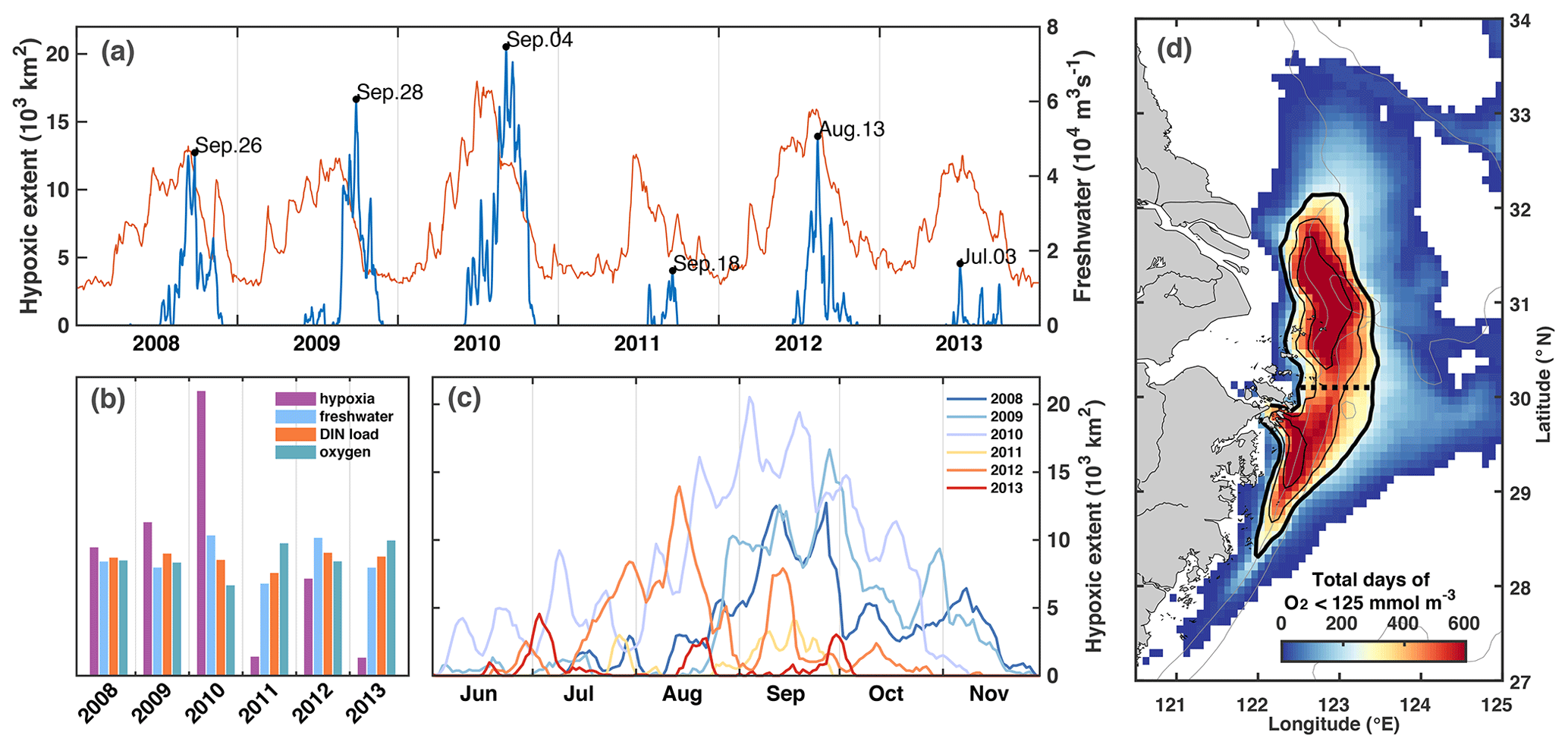
Figure 4(a) Time series of freshwater discharge (thin red line) and simulated hypoxic extent (thick blue line) with peaks specified by date. (b) Annual comparison of normalized time-integrated hypoxic extent, freshwater discharge, DIN load, and summer-mean bottom oxygen concentration. (c) Evolution of simulated hypoxic extent by year. (d) Frequency map of number of days when bottom oxygen concentrations were below 125 mmol m−3 (4mg L−1). The black isolines indicate 240, 360, and 480 d (or 40, 60, and 80 d yr−1). The thick solid line indicates the region we refer to as the typical low-oxygen zone, and the dashed line shows the demarcation between its northern and southern regions.
3.2.1 Interannual variations in hypoxia
The first question we address is, do year-to-year variations in nutrient load and FW input from the Changjiang explain interannual variability in hypoxic conditions? We do this by investigating correlations of time-integrated hypoxic area, average PP, total OC by respiration, SOC, and bottom oxygen in the typical low-oxygen zone (Fig. 5a–f). We also consider the correlation between the spatial extent of the FW plume, defined as the horizontal extent of surface water with salinity less than 29, and annually integrated FW input and DIN load (Fig. 5g–i).
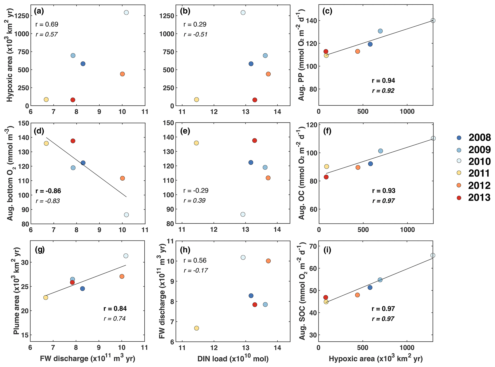
Figure 5Correlations of time-integrated hypoxic area, average primary production, respiration, and bottom oxygen in the typical low-oxygen zone in August, and the spatial extent of the FW plume (defined here as the area with surface salinity smaller than 29) with annually integrated FW input and DIN load. Correlation coefficients are given for all 6 years and, in italic font, after excluding the year 2011. Significant correlations are shown in bold font, and linear regressions are indicated by the black line where the correlation is significant at p<0.05.
There is a significant negative correlation between annual FW input and mean bottom-water oxygen concentration in the low-oxygen zone of −0.86 and a weaker, statistically insignificant positive correlation of 0.69 between annual FW input and integrated hypoxic area (Fig. 5a, d). This indicates that variations in FW input at least partly explain variability in hypoxic conditions. Perhaps surprisingly, there is no convincing correlation between annual FW input and annual DIN load (Fig. 5h). Although the correlation coefficient is 0.56 when all 6 years are considered, the correlation reverses to −0.17 when the low-flow year 2011 is excluded, and neither of these correlations is statistically significant. As expected, there is a strong positive correlation of 0.84 between the annual FW input and time-integrated plume area (Fig. 5g). Plume area can thus be interpreted as a proxy of FW input.
In contrast to the positive correlations between FW input and hypoxia, and FW input and bottom oxygen, correlations between the annual DIN load with integrated hypoxic area and mean bottom-water oxygen are much weaker and insignificant (Fig. 5b, e). This implies that interannual variations in DIN load do not lead to year-to-year variations in hypoxia. However, the correlations between integrated hypoxic area and mean rates of PP and OC (especially SOC) in August are significant and strong at 0.94 and 0.93 (0.97), respectively (Fig. 5c, f, i). The high correlation between hypoxic area and OC is primarily driven by SOC. Clearly, biological processes are important drivers of hypoxia and contribute to its interannual variability, but they do not appear to result from variations in DIN load. More relevant are variations in FW load, which explain interannual variations in hypoxia at least partly.
Other factors than riverine inputs of nutrients and FW must be contributing to interannual variations. For example, the years 2010 and 2012 both had very similar FW input and DIN load but differed in severity of hypoxia (Fig. 5a, b). Likewise, the years 2009 and 2013 were very similar in terms of FW input and DIN load but very different in hypoxic extent. Next, we investigate the potential reasons for shorter-term variability in hypoxia, i.e., the processes leading to the differences in hypoxia phenology in Fig. 4c.
3.2.2 Biological drivers of short-term variability in hypoxia
In the previous subsection, we identified biological rates as important drivers of low-oxygen conditions on interannual timescales but unrelated to variations in riverine DIN load. Here we attempt to elucidate what drives variations in biological rates and low-oxygen conditions on shorter timescales by addressing the following two questions. Do low-oxygen conditions correlate with biological rates on these shorter timescales? If yes, what drives variations in biological rates?
For this analysis it seems prudent to distinguish between the northern and southern hypoxic regions for the following reasons. The bathymetry in the northern zone is slightly deeper than in the southern zone (median depth of 28.5 m versus 24.6 m), and several biological rates with direct relevance to oxygen dynamics are different between the two zones (Fig. 6). During the summer months (June to September), PP, oxygen consumption in the water column (WOC = OC − SOC), and SOC are larger in the northern zone with medians of 124 compared to 77.0 mmol O2 m−2 d−1 for PP, of 43.1 versus 35.9 mmol O2 m−2 d−1 for WOC, and 49.3 versus 27.3 mmol O2 m−2 d−1 for SOC. During hypoxic conditions, PP and SOC are also notably larger in the northern zone with medians of 151 versus 107 mmol O2 m−2 d−1 for PP and 69.9 versus 50.4 mmol O2 m−2 d−1 for SOC. In the water column, the difference is reversed and WOC is larger in the southern than the northern zone (52.9 versus 46.7 mmol O2 m−2 d−1). Because of these different characteristics, we consider the northern and southern zones of the typical low-oxygen region separately.
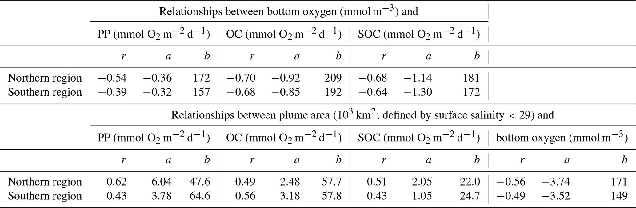
First, we explore whether significant relationships exist between daily biological rates and bottom-water oxygen by determining the correlations of daily averaged rates of PP, OC, and SOC with daily mean bottom oxygen concentration (Fig. 7 and Table 1).
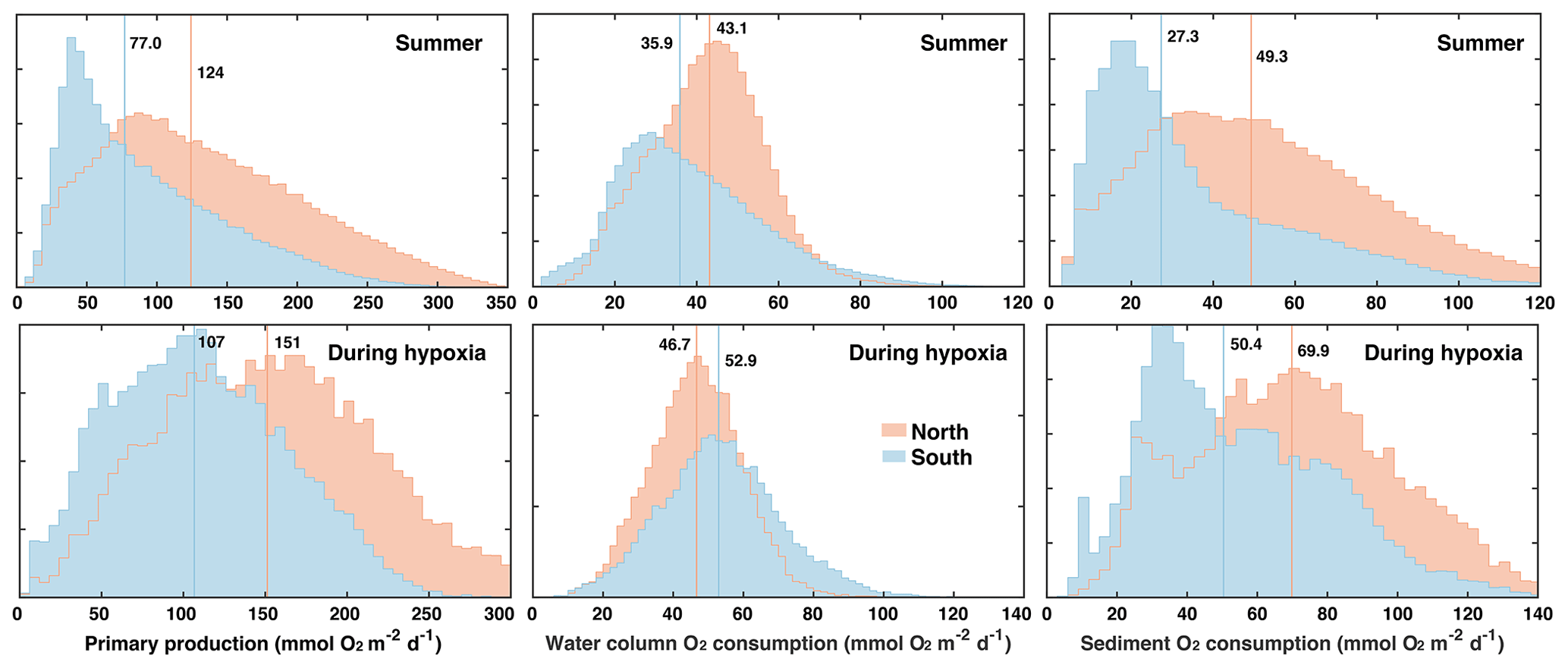
Figure 6Histograms of primary production and water-column and sediment respiration during the summer months (June to September) and during hypoxic conditions in the northern and southern parts of the typically hypoxic zone. Medians are indicated by vertical lines.
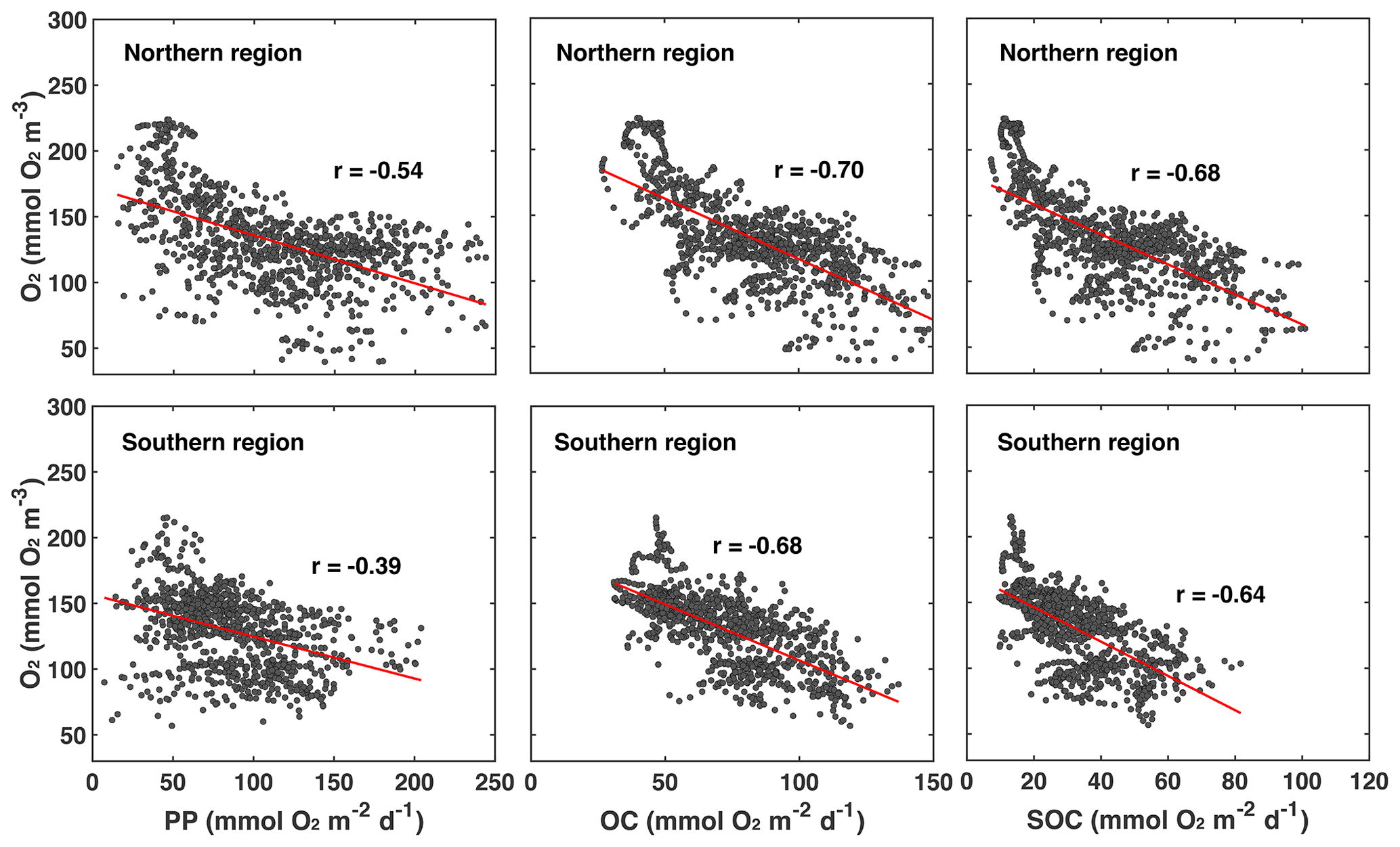
Figure 7Correlations of daily averaged rates of PP, OC, and SOC plotted with daily mean bottom oxygen concentration in the northern and southern regions of the low-oxygen zone in summer. The correlations are all significant. Correlation coefficients and slope and intercept of linear regressions (indicated by red lines) are given in Table 1.
Indeed, daily PP, OC, and SOC are all significantly and negatively correlated with bottom-water oxygen. This confirms that local production of organic matter and the resulting biological oxygen consumption are important for hypoxia development and that variations in these rates partly explain variations in low-oxygen conditions. However, it is also obvious that variability around the best fit is large (Fig. 7). The next question is, what drives variations in the biological rates? Since the annual correlations presented in the previous section indicate that variability in annual FW input partly explains interannual variability in hypoxia, we consider whether FW variability is related to variations in biological rates. Using daily plume extent as a measure of FW presence and comparing it to daily rates of PP, OC, SOC, and bottom oxygen, we find that bottom oxygen and biological rates are significantly correlated with the extent of the FW plume, with correlation coefficients ranging from 0.43 to 0.62 (Table 1). In other words, variability in the extent of the FW plume explains roughly half of the variability in biological rates. Mechanistically, the presence of a large FW plume affects hypoxia not only by increasing vertical stratification and thus inhibiting vertical supply of oxygen to the subsurface but also because PP and respiration are larger in the plume. Large FW plumes stimulate more widespread biological production and thus oxygen consumption.
Since annual FW input is highly correlated with the extent of the FW plume (see Fig. 5g), variability in its extent is partly due to variations in riverine input, but coastal circulation and mixing processes must be playing a role as well. Next, we analyze the impact of the underlying physical drivers.
Table 1Correlation coefficients and parameters of a linear model fit (of the form ) between bottom oxygen, FW plume area, PP, OC, and SOC in the northern and southern regions.
3.2.3 Physical drivers of short-term variability in hypoxia
We focus our analysis of physical drivers on wind direction and wind strength, and their relation to FW plume location and extent because the latter has already been identified as an explanatory variable for interannual variations in the previous section.
Wind direction is relevant because for most of June, July, and August winds blow predominantly from the south, but they switch to being predominantly northerly winds between the second half of August and the end of September. As a result of the northward, upwelling-favorable winds in the early summer, the FW plume is spread offshore and overlaps primarily with the northern zone. After the switch to mostly southward, downwelling-favorable directions, the FW plume moves southward, becomes more contained near the coast, and grows in its southward extent as it is transported by a coastal current. Wind direction has a demonstrable impact on PP and the extent of the FW plume as shown in Fig. 8 for the month of September. Especially in the northern region, PP and plume extent are notably larger during southerly winds, when the FW plume is more spread out, than during northerly winds, when the plume is more restricted within the coastal current.
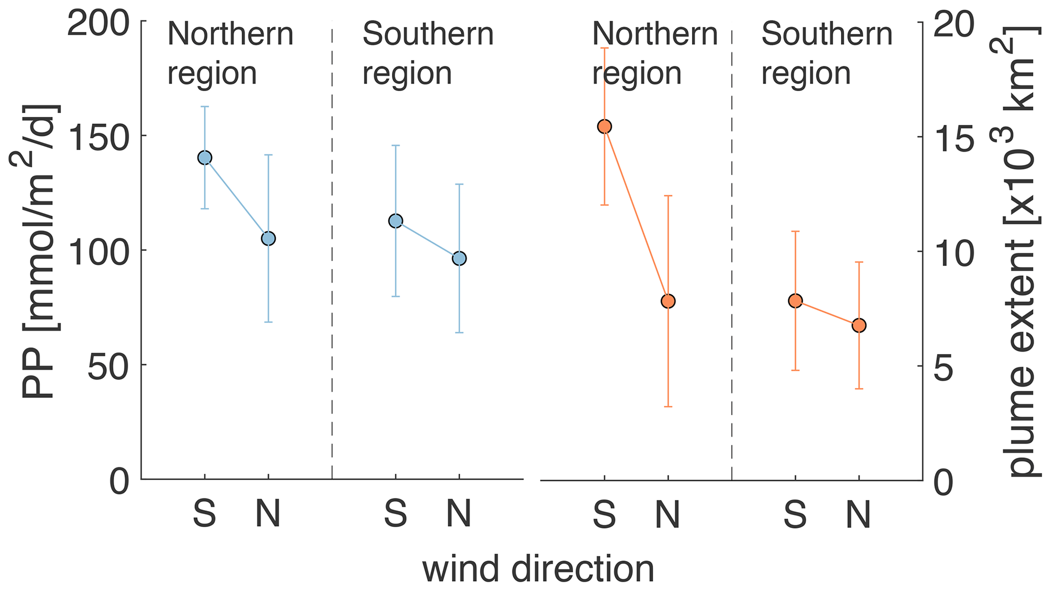
Figure 8Mean PP and FW plume extent in the northern and southern regions averaged over all days during the 6-year simulation with north and south wind (i.e., when direction is ± 45∘ of true north or south) and wind strength > 0.03 Pa in September.
Wind strength is relevant because storm events can erode vertical stratification and thus lead to resupply of oxygen to bottom waters due to vertical mixing. We investigated the effect of wind strength on bottom oxygen, hypoxia, and the extent of the FW plume by first inspecting time series of these variables (Fig. S8). We isolated all events during the months June to September and, in Fig. 10, show the corresponding changes in wind stress, mean bottom oxygen in the northern and southern zones, and the extent of the FW plume. We diagnosed these events as follows. First, we identified all days when the wind stress exceeded 0.12 Pa. Then we detected the minima in wind stress adjacent to the high-wind days by searching for minima in wind stress within 3 d prior to and 3 d after the high-wind days. The periods within these minima are used as an analysis period for each wind event. In four instances the wind stress exceeded the threshold within 5 d of a previous wind event. Those subsequent high-wind events were combined into one. We identified the minimum in bottom oxygen (maximum in FW plume area) at the beginning of the event and the maximum in oxygen (minimum in FW area) after the maximum in wind stress was reached.
Figure 9a illustrates rapid increases in wind stress typically within 2 to 4 d. The only exceptions are the four events where two storms occurred in rapid succession and the combined event lasted longer (up to 8 d) until maximum wind stress was reached. The year with the most wind events is 2013 (with eight in total including one of the combined long-lasting events). The year with the least events is 2010 (two events), followed by 2009 (three events). Most of these events resulted in notable increases in mean bottom oxygen, typically by 10 to 30 mmol m−3, but up to 100 mmol m−3 in 2010 in the southern zone (Fig. 9b). In the rare cases where bottom oxygen did not increase or slightly decreased, bottom oxygen was already elevated before the wind event. The wind events strongly affected the extent of the FW plume (Fig. 9c) by mixing the FW layer with underlying ocean water. The effects were largest when the FW plume was most expansive. This analysis shows the significant role of storm events in disrupting the generation of low-oxygen conditions and ventilating bottom waters.
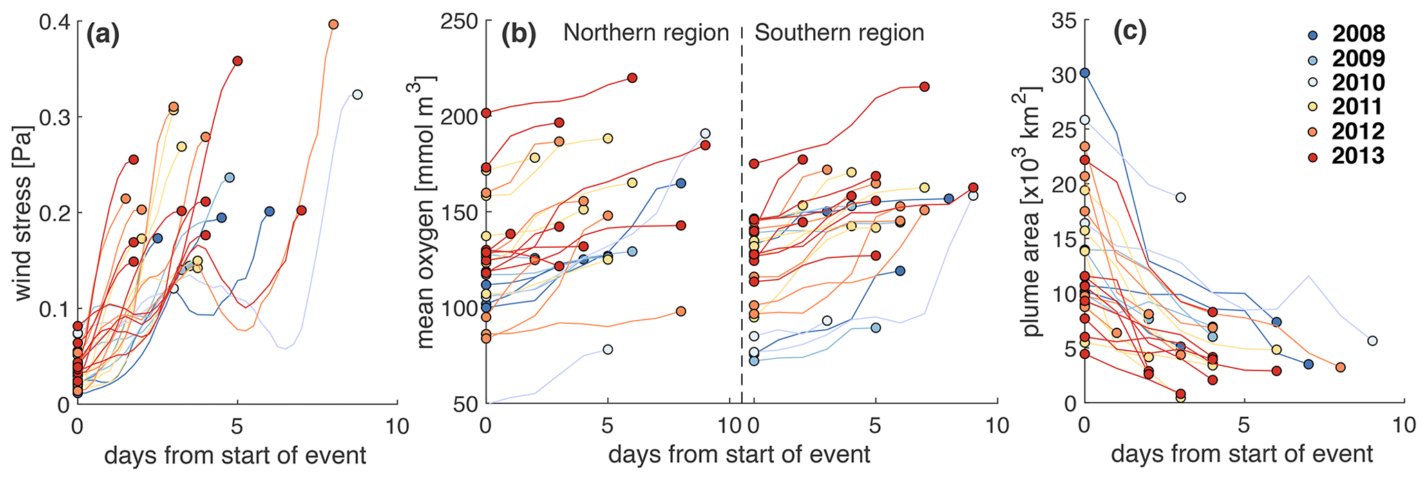
Figure 9Evolution of (a) wind stress, (b) bottom mean oxygen in the northern and southern regions, and (c) extent of the FW plume during high-wind events. These events are defined by wind stress exceeding 0.12 Pa.
In Sect. 3.2.1 above, where we discussed interannual variability, we noted that, while the years 2010 and 2012 had very similar FW input and DIN load, 2010 had a much larger hypoxic area. Likewise, the years 2009 and 2013 were very similar in terms of FW input and DIN load, but 2009 had a much larger hypoxic area. It now becomes obvious that the frequency and severity of high-wind events – i.e., variations on short timescales – explain the interannual differences in both cases.
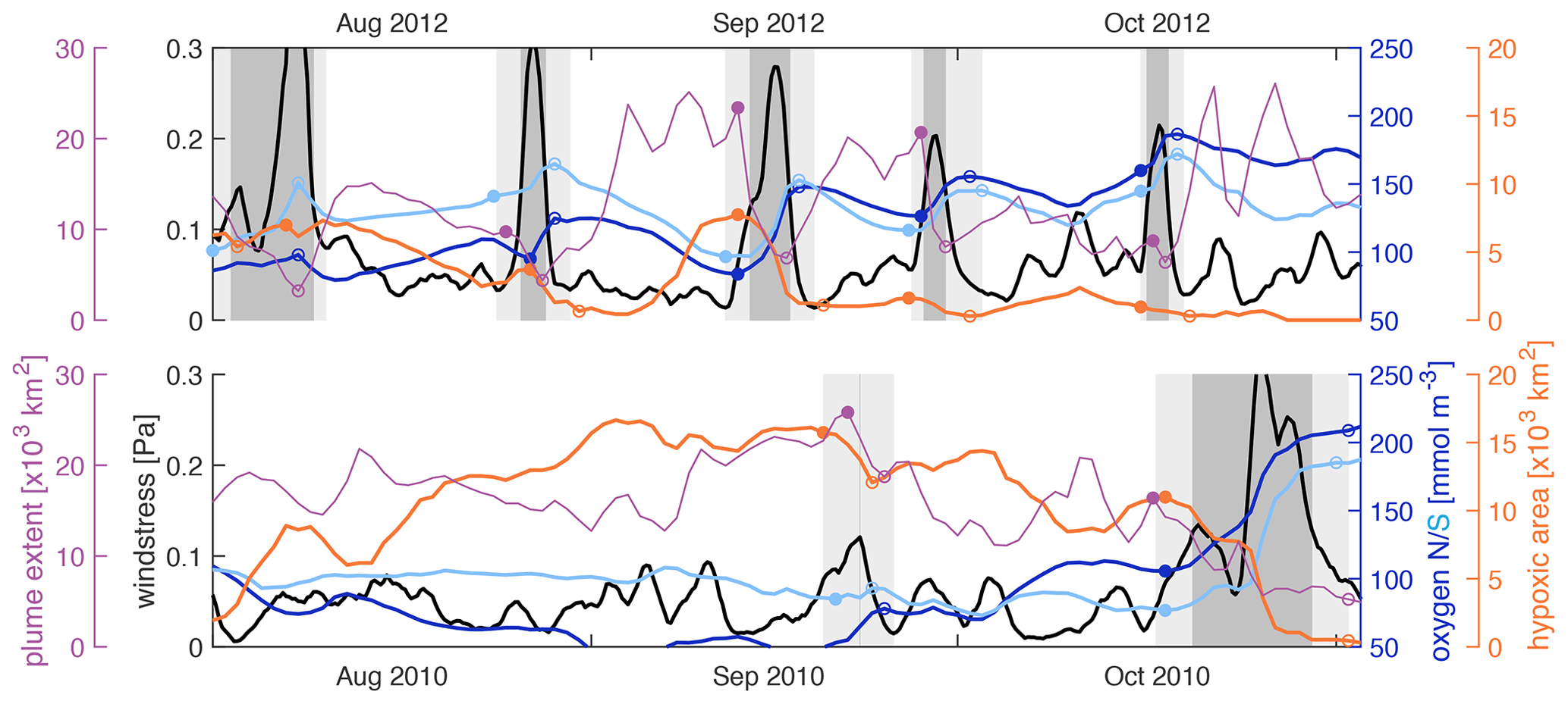
Figure 10Wind stress (black), mean bottom oxygen in the northern and southern zones (dark and light blue), total hypoxic extent (orange), and FW plume extent (purple) throughout August, September, and October of 2010 and 2012. The filled and open circles indicate a variable's value at the beginning and after high-wind events. High-wind days (events) are indicated by the dark (light) grey shading.
Figure 10 shows the wind stress, mean bottom oxygen in the northern and southern zones, and total hypoxic extent and FW plume extent in 2012 and 2010. In 2012, there were five high-wind events during the months of August, September, and October that all coincided with increases in bottom oxygen, decreases in hypoxic extent when a hypoxic zone was established at the beginning of the event, and decreases in FW plume extent. Inspection of the evolution of bottom oxygen is especially instructive. While bottom oxygen concentrations declined during periods with average or low wind, they were essentially reset at a much higher level during each wind event. Whenever the FW plume was extensive at the beginning of a high-wind event, it was drastically reduced during the event. In 2010, bottom oxygen was at similar levels to 2012 at the beginning of August but dropped to low levels throughout August, especially in the northern zone, and remained low with widespread hypoxia until a major wind event in the second half of October ventilated bottom waters. Except for a very short event in the second half of September, there were no high-wind events from August until mid-October in 2010.
The differences in hypoxia in 2009 and 2013 can also be explained by the frequency and intensity of high-wind events. In 2013, there were eight high-wind events from July to October that led to an almost continuous ventilation of bottom waters, while in 2009 there were only three such events during the same period (Fig. S8). Low to average winds from mid-August to early October of 2009 coincided with a decline in bottom oxygen and establishment of an expansive hypoxic zone throughout most of September.
These analyses show that wind direction and strength play an important role in determining the location of the hypoxic zone (i.e., northern versus southern region) and the extent and severity of hypoxic conditions.
In order to further investigate the roles of physical and biological processes in regulating hypoxia, oxygen budgets were calculated from daily model output for the period from March to November for the northern and southern hypoxic regions. Considering that hypoxic conditions occur near the bottom, we evaluate an oxygen budget not only for the whole water column but also for its lower portion, which typically becomes hypoxic. To account for variations in the thickness of the hypoxic layer, which tends to be thicker in deeper waters (similar to observations by Ning et al., 2011), we include the bottommost 12 layers of our model grid. Because of the model's terrain-following vertical coordinates, the thickness of these 12 model layers varies with total depth. The terms considered in the budget are air–sea flux, lateral physical advection and diffusion, vertical turbulent diffusion (for the subsurface budget only), PP, WOC (including respiration and nitrification), and SOC. Each term was integrated vertically over the whole water column and also over the bottom-most 12 layers and then averaged for the northern and southern regions for each month (Fig. 11). We also report these terms for the months during which oxygen decreases (March to August) in Table S2.
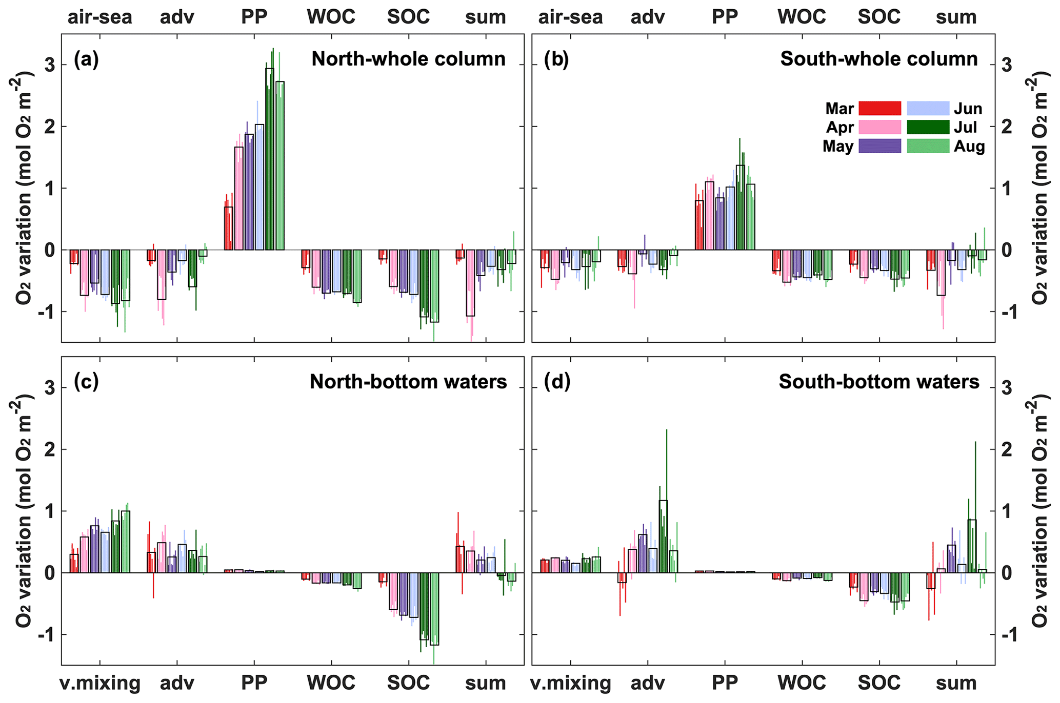
Figure 11Monthly averaged (2008–2013) oxygen budgets for the whole water column and subsurface water from March to November in the northern and southern hypoxic regions. Adv represents lateral advection and lateral diffusion, which is comparatively small, while v.mixing represents vertical turbulent diffusion, which is only relevant for the subsurface budget. Thin color bars represent individual years, whereas the black bars are the 6-year average.
For the whole water column (Fig. 11a, b), biological processes (PP, WOC, and SOC) greatly exceed physical processes (air–sea exchange and advective transport) in affecting oxygen. PP is always greater than the sum of WOC and SOC in the whole column, indicating autotrophy in spring and summer. Advection is negative, acting as an oxygen sink and offsetting 21 % of PP on average in the northern and southern regions. Of the two biological oxygen consumption terms (WOC and SOC), WOC accounts for half of total respiration. Negative air–sea flux indicates oxygen outgassing into the atmosphere and is due to photosynthetic oxygen production and decreasing oxygen solubility. However, since hypoxia only occurs in the subsurface, the subsurface budget below is more instructive. When considering only subsurface waters (Fig. 11c, d), the influence of PP decreases markedly, accounting for less than 2 % of that in the whole water column. Vertical turbulent diffusion acts as the largest oxygen source in the subsurface layer. SOC is the dominant oxygen sink, accounting for 80% of the total biological oxygen consumption. As photosynthetic oxygen production increases gradually from spring to summer (Fig. 12a, b), WOC and SOC also increase as they are closely associated with photosynthetically produced organic matter. Vertical oxygen diffusion tends to covary with PP, implying an oxygen gradient driven by photosynthetic oxygen production in the upper layer. Lateral advection of oxygen is negative in March only (early in the hypoxic season) mainly in the southern region but becomes positive later. This suggests that, early in the hypoxic season, import of low-oxygen water contributes to hypoxia generation but that advection switches to an oxygen source later. Overall, oxygen sources and sink terms are similar in the northern and southern regions.
We implemented and validated a state-of-the-art physical-biological model for the ECS. The implementation is based on a model that was previously developed and extensively used for the northern Gulf of Mexico (Fennel et al., 2011; Laurent et al., 2012; Yu at al., 2015b), a region that is similar to the ECS in that it receives large inputs of FW and nutrients from a major river and develops extensive, annually recurring hypoxia (see Table 1 in Fennel and Testa (2019). Our model is more comprehensive than previous models for the ECS.
A 6-year simulation was performed and compared to available observations. The model faithfully represents patterns and variability in surface and bottom temperature and salinity, surface chlorophyll and nitrate distributions, and bottom oxygen, and it correctly simulates the major current patterns in the region (see Sect. 3.1 and Supplement). We thus deem the model's skill as sufficient for the analysis of biological and physical drivers of hypoxia generation presented here.
The model simulates annually recurring hypoxic conditions but with significant interannual and short-term variability and marked differences in phenology of hypoxic conditions from year to year (Fig. 4a, b, c). Interannual variability in hypoxic conditions is much larger than variations in FW input, nutrient load, and bottom oxygen concentrations (Fig. 4b) because small variations in oxygen can lead to large changes in hypoxic area when bottom oxygen is near the hypoxic threshold. Interannual variability in the hypoxic area is partly explained by variations in annual FW input, consistent with previous studies (Zheng et al., 2016; Zhou et al., 2017). While the correlation between time-integrated hypoxic area and FW input is insignificant, there is a strong and significant negative correlation between mean bottom oxygen in August and annual FW input (Fig. 5). Annual FW input is also correlated strongly and significantly with the annually integrated spatial extent of the FW plume, which is a useful metric for the extent of the region directly influenced by riverine inputs which induce strong density stratification and high productivity.
Surprisingly, DIN load is not correlated with FW input, hypoxic area, or mean bottom oxygen in August (Fig. 5). This is in contrast to the northern Gulf of Mexico, where DIN load is highly correlated with both FW input and nutrient load and frequently used as a predictor of hypoxic extent (Scavia et al., 2017; Laurent and Fennel, 2019). However, the lack of correlation between hypoxia and DIN load in the ECS should not be interpreted as biological processes being unimportant in hypoxia generation, just that variations in DIN load do not explain year-to-year differences. In fact, hypoxic area and biological rates (i.e., mean August PP, OC, and SOC) are strongly and significantly correlated (Fig. 5), emphasizing the dominant role of biological oxygen consumption. The fact that riverine variations in DIN load do not seem to have an effect suggests that riverine nutrient inputs are large enough to saturate the region with nutrients, similar to the northern Gulf of Mexico, where small reductions in nutrient load have a relatively small effect (Fennel and Laurent, 2018).
Variations in riverine FW input only partly explain interannual variations in hypoxia. For example, the years 2010 and 2012 had similar FW inputs and DIN loads, but the hypoxic area was 4 times larger in 2010 than 2012 (Fig. 5a). Similarly, 2009 and 2013 had the same FW inputs and nutrient loads, but 2009 experienced extensive hypoxia, while there was almost none in 2013. In order to elucidate these differences, we investigated biological and physical drivers on shorter timescales.
In the ECS, two distinct zones of low oxygen have been observed (Li et al., 2002; Wei et al., 2007; Zhu et al., 2016, 2011). The model simulates these two zones, referred to as the northern and southern zones, consistent with observations (Fig. 4d) and with generally higher PP and SOC in the northern zone (Fig. 6). Because of these differences, we treated the two zones separately in our analysis of intra-seasonal drivers.
We found daily biological rates (i.e., PP, OC, and SOC) to be significantly correlated with bottom oxygen in both zones, but with relatively large variability around the best linear fit (Fig. 7). The biological rates and bottom oxygen are also significantly correlated with the extent of the FW plume (Table 1). Again, these results emphasize the dominant role of biological oxygen consumption, and its relation to riverine inputs, in hypoxia generation but leave a significant fraction of the variability unexplained.
Intra-seasonal variability in hypoxic conditions is significantly related to the extent of the FW plume, which is partly explained by variations in riverine FW input but strongly modulated by coastal circulation and mixing. Their influence is elucidated by our analysis of the effects of wind direction and strength on hypoxia. Wind direction has a notable effect on the geographic distribution of hypoxia. Southerly, upwelling-favorable winds lead to a more widespread eastward extension of the FW plume with elevated PP and vertical density stratification (Fig. 8). Northerly, downwelling-favorable winds create a coastally trapped southward jet that moves FW southward and constrains the plume close to the coast. Similar behavior has been described for the northern Gulf of Mexico (Feng et al., 2014).
Wind strength turned out to be one of the dominant factors in hypoxia evolution. We identified high-wind events and showed that whenever bottom oxygen is low the occurrence of a high-wind event will lead to a partial reoxygenation of bottom waters and decrease hypoxic extent (Fig. 9). The impact of high-wind events is also visible in the extent of the FW plume, which is drastically reduced during high winds because FW is mixed. The frequency of high-wind events during summer explains the interannual differences in hypoxic area between 2010 and 2012 (Fig. 10) and 2009 and 2013 (Fig. S8). In 2009 and 2010 there were only few high-wind events during summer, while 2012 and 2013 experienced a sequence of storms that led to partial reoxygenation of the water column throughout the summer and thus impeded the development of hypoxia.
We calculated oxygen budgets for the northern and southern regions considering the whole water column and the near-bottom layer only. The subsurface budget is particularly useful in providing insights into when and where lateral advection amplifies or mitigates hypoxia and illustrates that SOC is the dominant oxygen sink in the subsurface. The relative importance of WOC and SOC had not previously been quantified for this region due to lack of concurrent WOC and SOC observations and lack of models that realistically account for both processes. The budget for the whole water column is less useful because it is dominated by the oxygen sources, sinks, and transport in the surface layer, which does not experience hypoxia and thus is not relevant.
The importance of SOC suggested by our model is consistent with recent observational studies in the ECS. SOC on the coastal shelves in the Yellow Sea and ECS has been estimated to range from 1.7 to 17.6 mmol O2 m−2 d−1 (mean rate of 7.2 mmol O2 m−2 d−1) from April to October except August by Song et al. (2016), and from 9.1 to 62.5 mmol O2 m−2 d−1 (mean of 22.6 ± 16.4 mmol O2 m−2 d−1) from June to October by Zhang et al. (2017). Simulated SOC in the typical low-oxygen zone falls within the range observed by Zhang et al. (2017) with a mean rate of 20.6 ± 19.2 mmol O2 m−2 d−1 between April and October. Based on observations, Zhang et al. (2017) already suggested that SOC is a major contributor to hypoxia formation in below-pycnocline waters, which is further corroborated by our model results. It is also consistent with the modeling study of Zhou et al. (2017), who did not include SOC in the baseline version of their model but showed in a sensitivity study that inclusion of SOC simulates hypoxic extent more realistically. Our results are in line with findings from the northern Gulf of Mexico hypoxic zone, where WOC is much larger than SOC below the pycnocline, while SOC is dominant in the bottom 5 m, where hypoxia occurs most frequently in summer (Quiñones-Rivera et al., 2007; Yu et al., 2015b).
The finding that lateral oxygen transport can act as a net source to subsurface water is also new. On seasonal scales, oxygen advection in the subsurface varies from an oxygen sink in spring to a source in summer, especially in the southern hypoxic region, implying that the TWC becomes an oxygen source when oxygen is depleted in the hypoxic region. This aspect was neglected in previous studies, which only emphasized the role of advection as an oxygen sink promoting hypoxia formation (Ning et al., 2011; Qian et al., 2017). The Taiwan Warm Current originates from the subsurface of the Kuroshio Current northeast of Taiwan and thus represents an intrusion onto the continental shelves from the open ocean (Guo et al., 2006). In addition to oxygen advection, nutrients are transported, supporting PP on the ECS shelves (Zhao and Guo, 2011; Grosse et al., 2020). The intrusion of the Taiwan Warm Current and the Kuroshio Current accompanied by relatively cold and saline water, and nutrient and oxygen transport, is thought to influence hypoxia development (Li et al., 2002; Wang, 2009; Zhou et al., 2017), but no quantification of the relative importance has occurred until now (see companion paper by Grosse et al., 2020, using the same model).
In this study, a new 3D coupled physical-biological model for the ECS was presented and used to explore the spatial and temporal evolution of hypoxia off the CE and to quantify the major processes controlling interannual and intra-seasonal oxygen dynamics. Validation shows that the model reproduces the observed spatial distribution and temporal evolution of physical and biological variables well. A 6-year simulation with realistic forcing produced large interannual and intra-seasonal variability in hypoxic extent despite relatively modest variations in FW input and nutrient loads. The interannual variations are partly explained by variations in FW input but not DIN load. Nevertheless, elevated rates of biological oxygen consumption are of paramount importance for hypoxia generation in this region, as shown by the high correlation between hypoxic area, bottom oxygen, and biological rates (PP, OC, and SOC) on both annual and shorter timescales.
Other important explanatory variables of variability in hypoxia are wind direction and strength. Wind direction affects the magnitude of PP and the spatial extent of the FW plume, because southerly, upwelling-favorable winds tend to spread the plume over a large area while northerly, downwelling-favorable winds push the plume against the coast and induce a coastal current that contains the FW and moves it downcoast. Wind strength is important because high-wind events lead to a partial reoxygenation whenever bottom oxygen is low and can dramatically decrease the extent of the FW plume. The frequency of high-wind events explains some of the interannual differences in hypoxia, where years with similar FW input, nutrient load, and mean rates of oxygen consumption display very different hypoxic extents because high-wind events lead to partial reoxygenation of bottom waters.
A model-derived oxygen budget shows that SOC is larger than WOC in the subsurface of the hypoxic region. Lateral advection of oxygen in the subsurface switches from an oxygen sink in spring to a source in summer especially in the southern region and is likely associated with open-ocean intrusions onto the coastal shelf supplied by the Taiwan Warm Current.
ROMS source code, http://myroms.org, last access: 10 August 2019 (Haidvogel et al., 2008); AVHRR SST, https://www.nodc.noaa.gov/SatelliteData/ghrsst/, last access: 10 August 2019; MODIS-Terra sea surface chlorophyll, https://oceandata.sci.gsfc.nasa.gov/MODIS-Terra/, last access: 10 August 2019. Model results are available on request.
The supplement related to this article is available online at: https://doi.org/10.5194/bg-17-5745-2020-supplement.
The paper is based on HZ's PhD thesis (in Chinese). CB implemented the physical model. HZ added the biological component, performed model simulations, and wrote the first version of the manuscript with input from KF and AL. For the manuscript revisions, AL reran the model simulation, AL and KF performed additional analyses, and KF revised the text.
The authors declare that they have no conflict of interest.
This article is part of the special issue “Ocean deoxygenation: drivers and consequences – past, present and future (BG/CP/OS inter-journal SI)”. It is not associated with a conference.
We thank the crew of the Dongfanghong2 for help during the cruises and Compute Canada for supercomputer time.
This research has been supported by the National Key Research and Development Program of China (grant nos. 2016YFC1401602 and 2017YFC1404403) and the NSERC Discovery Grant (grant no. RGPIN-2014-03938).
This paper was edited by Andreas Oschlies and reviewed by three anonymous referees.
Baird, D., Christian, R. R., Peterson, C. H., and Johnson, G. A.: Consequences of hypoxia on estuarine ecosystem function: Energy diversion from consumers to microbes, Ecol. Appl., 14, 805–822, https://doi.org/10.1890/02-5094, 2004.
Bian, C., Jiang, W., and Greatbatch, R. J.: An exploratory model study of sediment transport sources and deposits in the Bohai Sea, Yellow Sea, and East China Sea, J. Geophys. Res.-Ocean., 118, 5908–5923, https://doi.org/10.1002/2013JC009116, 2013a.
Bian, C., Jiang, W., Quan, Q., Wang, T., Greatbatch, R. J., and Li, W.: Distributions of suspended sediment concentration in the Yellow Sea and the East China Sea based on field surveys during the four seasons of 2011, J. Mar. Syst., 121/122, 24–35, https://doi.org/10.1016/j.jmarsys.2013.03.013, 2013b.
Bianchi, T. S., DiMarco, S. F., Cowan, J. H., Hetland, R. D., Chapman, P., Day, J. W., and Allison, M. A.: The science of hypoxia in the northern Gulf of Mexico: A review, Sci. Total Environ., 408, 1471–1484, https://doi.org/10.1016/j.scitotenv.2009.11.047, 2010.
Bishop, M. J., Powers, S. P., Porter, H. J., and Peterson, C. H.: Benthic biological effects of seasonal hypoxia in a eutrophic estuary predate rapid coastal development, Estuar. Coast. Shelf Sci., 70, 415–422, https://doi.org/10.1016/j.ecss.2006.06.031, 2006.
Capet, A., Beckers, J. M., and Gregoire, M.: Drivers, mechanisms and long-term variability of seasonal hypoxia on the Black Sea northwestern shelf – Is there any recovery after eutrophication? Biogeosciences, 10, 3943–3962, https://doi.org/10.5194/bg-10-3943-2013, 2013.
Carton, J. A. and Giese, B. S.: A Reanalysis of Ocean Climate Using Simple Ocean Data Assimilation (SODA), Mon. Weather Rev., 136, 2999–3017, https://doi.org/10.1175/2007MWR1978.1, 2008.
Chen, C. C., Gong, G. C., and Shiah, F. K.: Hypoxia in the East China Sea: One of the largest coastal low-oxygen areas in the world, Mar. Environ. Res., 64, 399–408, https://doi.org/10.1016/j.marenvres.2007.01.007, 2007.
Chen, J., Cui, T., Ishizaka, J., and Lin, C.: A neural network model for remote sensing of diffuse attenuation coefficient in global oceanic and coastal waters: Exemplifying the applicability of the model to the coastal regions in Eastern China Seas, Remote Sens. Environ., 148, 168–177, https://doi.org/10.1016/j.rse.2014.02.019, 2014.
Chen, X., Shen, Z., Li, Y., and Yang, Y.: Physical controls of hypoxia in waters adjacent to the Yangtze Estuary: A numerical modeling study, Mar. Pollut. Bull., 97, 349–364, https://doi.org/10.1016/j.marpolbul.2015.05.067, 2015a.
Chen, X., Shen, Z., Li, Y., and Yang, Y.: Tidal modulation of the hypoxia adjacent to the Yangtze Estuary in summer, Mar. Pollut. Bull., 100, 453–463, https://doi.org/10.1016/j.marpolbul.2015.08.005, 2015b.
Dee, D. P., Uppala, S. M., Simmons, A. J., Berrisford, P., Poli, P., Kobayashi, S., and Vitart, F.: The ERA-Interim reanalysis: Configuration and performance of the data assimilation system, Q. J. Roy. Meteorol. Soc., 137, 553–597, https://doi.org/10.1002/qj.828, 2011.
Diaz, R. J. and Rosenberg, R.: Spreading dead zones and consequences for marine ecosystems, Science, 321, 926–929, https://doi.org/10.1126/science.1156401, 2008.
Egbert, G. D. and Erofeeva, S. Y.: Efficient inverse modeling of barotropic ocean tides, J. Atmos. Ocean. Technol., 19, 183–204, https://doi.org/10.1175/1520-0426(2002)019<0183:EIMOBO>2.0.CO;2, 2002.
Feng, Y., Fennel, K., Jackson, G. A., DiMarco, S. F., and Hetland, R. D.: A model study of the response of hypoxia to upwelling favorable wind on the northern Gulf of Mexico shelf, J. Mar. Syst., 131, 63–73, 2014.
Fennel, K. and Laurent, A.: N and P as ultimate and proximate limiting nutrients in the northern Gulf of Mexico: implications for hypoxia reduction strategies, Biogeosciences, 15, 3121–3131, https://doi.org/10.5194/bg-15-3121-2018, 2018.
Fennel, K. and Testa, J. M.: Biogeochemical controls on coastal hypoxia, Ann. Rev. Mar. Sci., 11, 105–130, https://doi.org/10.1146/annurev-marine-010318-095138, 2019.
Fennel, K., Wilkin, J., Levin, J., Moisan, J., O'Reilly, J., and Haidvogel, D.: Nitrogen cycling in the Middle Atlantic Bight: Results from a three-dimensional model and implications for the North Atlantic nitrogen budget, Global Biogeochem. Cy., 20, 1–14, https://doi.org/10.1029/2005GB002456, 2006.
Fennel, K., Hetland, R., Feng, Y., and DiMarco, S.: A coupled physical-biological model of the Northern Gulf of Mexico shelf: Model description, validation and analysis of phytoplankton variability, Biogeosciences, 8, 1881–1899, https://doi.org/10.5194/bg-8-1881-2011, 2011.
Fennel, K., Hu, J., Laurent, A., Marta-Almeida, M., and Hetland, R.: Sensitivity of hypoxia predictions for the northern Gulf of Mexico to sediment oxygen consumption and model nesting, J. Geophys. Res.-Ocean., 118, 990–1002, https://doi.org/10.1002/jgrc.20077, 2013.
Garcia, H. E., Boyer, T. P., Locarnini, R. A., Antonov, J. I., Mishonov, A. V., Baranova, O. K., Zweng, M. M., Reagan, J. R., Johnson, D. R., and Levitus, S.: World Ocean Atlas 2013, Vol. 3, Dissolved oxygen, apparent oxygen utilization, and oxygen saturation, Tech. rep., National Oceanic and Atmospheric Administration (NOAA), Silver Spring, MD, https://doi.org/10.7289/V5XG9P2W, 2013a.
Garcia, H. E., Locarnini, R. A., Boyer, T. P., Antonov, J. I., Baranova, O. K., Zweng, M. M., Reagan, J. R., Johnson, D. R., Mishonov, A. V., and Levitus, S.: World Ocean Atlas 2013, Vol. 4, Dissolved inorganic nutrients (phosphate, nitrate, silicate), Tech. rep., National Oceanic and Atmospheric Administration (NOAA), Silver Spring, MD, https://doi.org/10.7289/V5J67DWD, 2013b.
Grosse, F., Fennel, K., Zhang, H., and Laurent, A.: Quantifying the contributions of riverine vs. oceanic nitrogen to hypoxia in the East China Sea, Biogeosciences, 17, 2701–2714, https://doi.org/10.5194/bg-17-2701-2020, 2020.
Guo, X., Miyazawa, Y., and Yamagata, T.: The Kuroshio Onshore Intrusion along the Shelf Break of the East China Sea: The Origin of the Tsushima Warm Current, J. Phys. Oceanogr., 36, 2205–2231, https://doi.org/10.1175/JPO2976.1, 2006.
Haidvogel, D. B., Arango, H., Budgell, W. P., Cornuelle, B. D., Curchitser, E., Di Lorenzo, E., and Wilkin, J.: Ocean forecasting in terrain-following coordinates: Formulation and skill assessment of the Regional Ocean Modeling System, J. Comput. Phys., 227, 3595–3624, https://doi.org/10.1016/j.jcp.2007.06.016, 2008.
Laurent, A. and Fennel, K.: Simulated reduction of hypoxia in the northern Gulf of Mexico due to phosphorus limitation, Elementa, 2, 000022, https://doi.org/10.12952/journal.elementa.000022, 2014.
Laurent, A. and Fennel, K.: Time-evolving, spatially explicit forecasts of the northern Gulf of Mexico hypoxic zone, Environ. Sci. Technol., 53, 14449–14458, https://doi.org/10.1021/acs.est.9b05790, 2019.
Laurent, A., Fennel, K., Hu, J., and Hetland, R.: Simulating the effects of phosphorus limitation in the Mississippi and Atchafalaya river plumes, Biogeosciences, 9, 4707–4723, https://doi.org/10.5194/bg-9-4707-2012, 2012.
Laurent, A., Fennel, K., Cai, W.-J., Huang, W.-J., Barbero, L., and Wanninkhof, R.: Eutrophication-Induced Acidification of Coastal Waters in the Northern Gulf of Mexico: Insights into Origin and Processes from a Coupled Physical-Biogeochemical, Model. Geophys. Res. Lett., 44, 946–956, https://doi.org/10.1002/2016GL071881, 2017.
Li, D., Zhang, J., Huang, D., Wu, Y., and Liang, J.: Oxygen depletion off the Changjiang (Yangtze River) Estuary, Sci. China Ser. D, 45, 1137, https://doi.org/10.1360/02yd9110, 2002.
Li, H. M., Tang, H. J., Shi, X. Y., Zhang, C. S., and Wang, X. L.: Increased nutrient loads from the Changjiang (Yangtze) River have led to increased Harmful Algal Blooms, Harmful Algae, 39, 92–101, https://doi.org/10.1016/j.hal.2014.07.002, 2014.
Li, M., Lee, Y. J., Testa, J. M., Li, Y., Ni, W., Kemp, W. M., and Di Toro, D. M.: What drives interannual variability of hypoxia in Chesapeake Bay: Climate forcing versus nutrient loading?, Geophys. Res. Lett., 43, 2127–2134, https://doi.org/10.1002/2015GL067334, 2016.
Li, X., Bianchi, T. S., Yang, Z., Osterman, L. E., Allison, M. A., DiMarco, S. F., and Yang, G.: Historical trends of hypoxia in Changjiang River estuary: Applications of chemical biomarkers and microfossils, J. Mar. Syst., 86, 57–68, https://doi.org/10.1016/j.jmarsys.2011.02.003, 2011.
Liu, K. K., Yan, W., Lee, H. J., Chao, S. Y., Gong, G. C., and Yeh, T. Y.: Impacts of increasing dissolved inorganic nitrogen discharged from Changjiang on primary production and seafloor oxygen demand in the East China Sea from 1970 to 2002, J. Mar. Syst., 141, 200–217, https://doi.org/10.1016/j.jmarsys.2014.07.022, 2015.
Liu, S. M., Zhang, J., Chen, H. T., Wu, Y., Xiong, H., and Zhang, Z. F.: Nutrients in the Changjiang and its tributaries, Biogeochemistry, 62, 1–18, 2003.
Liu, S. M., Hong, G.-H., Ye, X. W., Zhang, J., and Jiang, X. L.: Liu, S. M., Hong, G.-H., Zhang, J., Ye, X. W., and Jiang, X. L.: Nutrient budgets for large Chinese estuaries, Biogeosciences, 6, 2245–2263, https://doi.org/10.5194/bg-6-2245-2009, 2009.
Locarnini, R. A., Mishonov, A. V., Antonov, J. I., Boyer, T. P., Garcia, H. E., Baranova, O. K., and Seidov, D.: World Ocean Atlas 2013, Vol. 1, Temperature, edited by: Levitus, S., A. Mishonov, Technical Ed.; NOAA Atlas NESDIS, 73, 40, https://doi.org/10.1182/blood-2011-06-357442, 2013.
Ning, X., Lin, C., Su, J., Liu, C., Hao, Q., and Le, F.: Long-term changes of dissolved oxygen, hypoxia, and the responses of the ecosystems in the East China Sea from 1975 to 1995, J. Oceanogr., 67, 59–75, https://doi.org/10.1007/s10872-011-0006-7, 2011.
Peña, A., Katsev, S., Oguz, T., and Gilbert, D.: Modeling dissolved oxygen dynamics and hypoxia, Biogeosciences, 7, 933–957, https://doi.org/10.5194/bg-7-933-2010, 2010.
Qian, W., Dai, M., Xu, M., Kao, S., Ji, Du, C., Liu, J., and Wang, L.: Non-local drivers of the summer hypoxia in the East China Sea off the Changjiang Estuary. Estuarine, Coast. Shelf Sci., 198, 393–399, https://doi.org/10.1016/j.ecss.2016.08.032, 2015.
Quiñones-Rivera, Z. J., Wissel, B., Justic, D., and Fry, B.: Partitioning oxygen sources and sinks in a stratified, eutrophic coastal ecosystem using stable oxygen isotopes, Mar. Ecol. Prog. Ser., 342, 69–83, https://doi.org/10.3354/meps342069, 2007.
Rabalais, N. N., Diaz, R. J., Levin, L. A., Turner, R. E., Gilbert, D., and Zhang, J.: Dynamics and distribution of natural and human-caused hypoxia, Biogeosciences, 7, 585–619, https://doi.org/10.5194/bg-7-585-2010, 2010.
Scavia, D., Bertani, I., Obenour, D. R., Turner, R. E., Forrest, D. R., and Katin, A.: Ensemble modeling informs hypoxia management in the northern Gulf of Mexico, P. Natl. Acad. Sci. USA, 114, 8823–8828, 2017.
Scully, M. E.: Physical controls on hypoxia in Chesapeake Bay: A numerical modeling study, J. Geophys. Res.-Ocean., 118, 1239–1256, https://doi.org/10.1002/jgrc.20138, 2013.
Smolarkiewicz, P. K. and Margolin, L. G.: MPDATA: A finite-difference solver for geophysical flows, J. Comput. Phys., 140, 459–480, 1998.
Song, G., Liu, S., Zhu, Z., Zhai, W., Zhu, C., and Zhang, J.: Sediment oxygen consumption and benthic organic carbon mineralization on the continental shelves of the East China Sea and the Yellow Sea, Deep-Sea Res. Pt. II, 124, 53–63, https://doi.org/10.1016/j.dsr2.2015.04.012, 2016.
Tong, Y., Zhao, Y., Zhen, G., Chi, J., Liu, X., Lu, Y., and Zhang, W.: Nutrient Loads Flowing into Coastal Waters from the Main Rivers of China (2006–2012), Sci. Rep., 5, 16678, https://doi.org/10.1038/srep16678, 2015.
Umlauf, L. and Burchard, H.: A generic length-scale equation for geophysical, J. Mar. Res., 61, 235–265, https://doi.org/10.1357/002224003322005087, 2003.
Wang, B.: Hydromorphological mechanisms leading to hypoxia off the Changjiang estuary, Mar. Environ. Res., 67, 53–58, https://doi.org/10.1016/j.marenvres.2008.11.001, 2009.
Wang, H., Dai, M., Liu, J., Kao, S. J., Zhang, C., Cai, W. J., and Sun, Z.: Eutrophication-Driven Hypoxia in the East China Sea off the Changjiang Estuary, Environ. Sci. Technol., 50, 2255–2263, https://doi.org/10.1021/acs.est.5b06211, 2016.
Wang, J., Yan, W., Chen, N., Li, X., and Liu, L.: Modeled long-term changes of DIN:DIP ratio in the Changjiang River in relation to Chl-a and DO concentrations in adjacent estuary, Estuar. Coast. Shelf Sci., 166, 153–160, https://doi.org/10.1016/j.ecss.2014.11.028, 2015.
Wei, H., He, Y., Li, Q., Liu, Z., and Wang, H.: Summer hypoxia adjacent to the Changjiang Estuary, J. Mar. Syst., 67, 292–303, https://doi.org/10.1016/j.jmarsys.2006.04.014, 2007.
Wei, H., Luo, X., Zhao, Y., and Zhao, L.: Intraseasonal variation in the salinity of the Yellow and East China Seas in the summers of 2011, 2012, and 2013, Hydrobiologia, 754, 13–28, https://doi.org/10.1007/s10750-014-2133-9, 2015.
Wu, R. S. S.: Hypoxia: From molecular responses to ecosystem responses, Mar. Pollut. Bull., 45, 35–45, https://doi.org/10.1016/S0025-326X(02)00061-9, 2002.
Yu, L., Fennel, K., and Laurent, A.: A modeling study of physical controls on hypoxia generation in the northern Gulf of Mexico, J. Geophys. Res.-Ocean., 120, 5019–5039, https://doi.org/10.1002/2014JC010634, 2015a.
Yu, L., Fennel, K., Laurent, A., Murrell, M. C., and Lehrter, J. C.: Numerical analysis of the primary processes controlling oxygen dynamics on the Louisiana shelf, Biogeosciences, 12, 2063–2076, https://doi.org/10.5194/bg-12-2063-2015, 2015b.
Yuan, D., Zhu, J., Li, C., and Hu, D.: Cross-shelf circulation in the Yellow and East China Seas indicated by MODIS satellite observations, J. Mar. Syst., 70, 134–149, https://doi.org/10.1016/j.jmarsys.2007.04.002, 2008.
Zhang, H., Zhao, L., Sun, Y., Wang, J., and Wei, H.: Contribution of sediment oxygen demand to hypoxia development off the Changjiang Estuary, Estuar. Coast. Shelf Sci., 192, 149–157, https://doi.org/10.1016/j.ecss.2017.05.006, 2017.
Zhang, J.: Nutrient elements in large Chinese estuaries, Cont. Shelf Res., 16, 1023–1045, https://doi.org/10.1016/0278-4343(95)00055-0, 1996.
Zhao, L. and Guo, X.: Influence of cross-shelf water transport on nutrients and phytoplankton in the East China Sea: A model study, Ocean Sci., 7, 27–43, https://doi.org/10.5194/os-7-27-2011, 2011.
Zheng, J., Gao, S., Liu, G., Wang, H., and Zhu, X.: Modeling the impact of river discharge and wind on the hypoxia off Yangtze Estuary, Nat. Hazards Earth Syst. Sci., 16, 2559–2576, https://doi.org/10.5194/nhess-16-2559-2016, 2016.
Zhou, F., Chai, F., Huang, D., Xue, H., Chen, J., Xiu, P., and Wang, K.: Investigation of hypoxia off the Changjiang Estuary using a coupled model of ROMS-CoSiNE, Prog. Oceanogr., 159, 237–254, https://doi.org/10.1016/j.pocean.2017.10.008, 2017.
Zhu, J., Zhu, Z., Lin, J., Wu, H., and Zhang, J.: Distribution of hypoxia and pycnocline off the Changjiang Estuary, China, J. Mar. Syst., 154, 28–40, https://doi.org/10.1016/j.jmarsys.2015.05.002, 2016.
Zhu, Z.-Y., Zhang, J., Wu, Y., Zhang, Y.-Y., Lin, J., and Liu, S.-M.: Hypoxia off the Changjiang (Yangtze River) Estuary: Oxygen depletion and organic matter decomposition, Mar. Chem., 125, 108–116, https://doi.org/10.1016/j.marchem.2011.03.005, 2011.
Zweng, M. M., Reagan, J. R., Antonov, J. I., Locarnini, R. A., Mishonov, A. V., Boyer, T. P., Garcia, H. E., Baranova, O. K., Johnson, D. R., Seidov, D., Biddle, M. M., and Levitus, S.: World Ocean Atlas 2013. Volume 2: Salinity, Tech. rep., National Oceanic and Atmospheric Administration (NOAA), Silver Spring, MD, https://doi.org/10.7289/V5251G4D, 2013.