Robust processing of airborne laser scans to plant area density profiles

We present a new algorithm for the estimation of the plant area density (PAD) profiles and plant area index (PAI) for forested areas based on data from airborne lidar.

The new element in the algorithm is to scale and average returned lidar intensities for each lidar pulse, whereas other methods do not use the intensity information at all, use only average intensity values, or do not scale the intensity information, which can cause problems for heterogeneous vegetation. We compare the performance of the new algorithm to three previously published algorithms over two contrasting types of forest: a boreal coniferous forest with a relatively open structure and a dense beech forest. For the beech forest site, both summer (full-leaf) and winter (bare-tree) scans are analyzed, thereby testing the algorithm over a wide spectrum of PAIs.

Whereas all tested algorithms give qualitatively similar results, absolute differences are large (up to 400 % for the average PAI at one site). A comparison with ground-based estimates shows that the new algorithm performs well for the tested sites. Specific weak points regarding the estimation of the PAD from airborne lidar data are addressed including the influence of ground reflections and the effect of small-scale heterogeneity, and we show how the effect of these points is reduced in the new algorithm, by combining benefits of earlier algorithms. We further show that low-resolution gridding of the PAD will lead to a negative bias in the resulting estimate according to Jensen's inequality for convex functions and that the severity of this bias is method dependent. As a result, the PAI magnitude as well as heterogeneity scales should be carefully considered when setting the resolution for the PAD gridding of airborne lidar scans.

1 Introduction

Plant area is a key parameter for the quantification of air–vegetation exchange of momentum, latent and sensible heat, and carbon dioxide. Its vertical distribution, the plant area density (PAD), describes the distribution of plant elements from the ground to the canopy top. The PAD profile is a key parameter in high-accuracy atmospheric models for the estimation of fluxes between the atmosphere and canopies (Williams et al., 1996; Sogachev et al., 2002; Patton et al., 2016; Smallman et al., 2013). PAD profiles have also been introduced into the modeling of wind over heterogeneous forests in the context of understanding how local inhomogeneities affect the wind field above the crowns (Boudreault et al., 2015; Ivanell et al., 2018). As wind turbines are very tall, the wind approaching the turbine is affected by surface conditions from far away. Therefore, large areas of consistent high-quality PAD profiles are attractive as model input. Likewise, atmosphere–biosphere interactions for weather and climate modeling require PAD information from large areas. With the advent of airborne lidar scans (ALSs), such a product is possible to achieve.

ALSs, made with a density of 5–10 laser shots over each square meter of ground, are now performed routinely on a country-level scale. Besides information on where the laser beam from the airplane was reflected in x, y, and z coordinates down to centimeter precision, each point is associated with several other attributes; these normally include the scanning angle, the number of returns from a pulse, the return rank in the pulse, and the intensity of the return. In this paper, we attempt to use more of this information than previously published methods (Solberg et al., 2006; Morsdorf et al., 2006; Richardson et al., 2009; Boudreault et al., 2015; Almeida et al., 2019; Hopkinson and Chasmer, 2009; Vincent et al., 2017) with the aim of producing a more consistent and less biased estimate of the PAD.

Previously established methods for calculating the PAD profile and, hence, the PAI from ALSs have been based on approximations of the Beer–Lambert law, which was first introduced in the field of vegetation density estimation by Monsi and Saeki in 1953 (see Monsi and Saeki, 2005, for a translated version). The results have been promising for the PAI (Solberg et al., 2006; Morsdorf et al., 2006; Richardson et al., 2009; Hopkinson and Chasmer, 2009) and even for PAD (Boudreault et al., 2015; Vincent et al., 2017; Almeida et al., 2019) calculations by ALSs when compared with various ground-based methods. The potential of estimating PAI and PAD from ALSs is underlined by relative agreement with ground-based methods made using very different techniques as well as the obvious advantage of producing results with great spatial coverage. Below, we recall the Beer–Lambert law and its adaptation for vegetative canopies and describe three reference models published by Hopkinson and Chasmer (2009), Boudreault et al. (2015), and Almeida et al. (2019). We then introduce the new method. The rest of the paper follows standard formats.

2 Background

2.1 The Beer–Lambert law and its adaptation for vegetative canopies

The Beer–Lambert law expresses the light level at a given height as a function of effective canopy density in the form of PAD as follows:

$$\begin{array}{}\text{(1)}& Q\left(z\right)=Q_{\mathrm{0}}{e}^{\frac{-\mathit{\mu }}{\cos \mathit{\theta }}{\int }_z^{h_{\mathrm{c}}}\mathrm{PAD}\left(z\right)\mathrm{d}z},\end{array}$$

where Q is the amount of radiation that penetrates the canopy to height z, Q₀ is the incoming radiation, μ is the extinction coefficient, θ is the zenith angle of the incoming radiation, and h_c is the height of the canopy. The value of μ depends on how the canopy elements are oriented in space, and the values for common types of trees have been reported to be in the range from 0.28 to 0.58 (see Bréda, 2003, for a detailed investigation). By rearranging Eq. (1), the PAD can be isolated and light-level observations can provide a basis for estimations of vegetation density.

In contrast to ground-based optical methods, measurements from ALSs are based on the reflected radiation R. Whereas it is clear from Eq. (1) that the radiation level above the canopy Q₀ is of high importance for the determination of the PAD and PAI, the use of the reflected radiation turns the problem on its head. To determine the value of the PAI based on ALS data, ground reflections are essential, and the magnitude of incoming radiation is not important for the PAI or the PAD provided that it is strong enough to produce detectable scatter at ground level. There are several other fundamental differences between the ground-based optical methods for determining the PAI and the lidar-based methods: (1) whereas optical methods are typically based on observed radiation of natural light, ALSs normally use infrared light; (2) the primary information utilized in ALS-based methods is the exact location describing where the radiation is reflected (e.g., Morsdorf et al., 2006; Solberg et al., 2006); and (3) contrary to the homogeneously lit canopies used to determine plant area with ground-based optical methods (Monsi and Saeki, 2005; Bréda, 2003; Yan et al., 2019), ALS data are based on discrete lidar pulses, which have a finite diameter of around 0.1–1 m at the canopy top (e.g., Hopkinson and Chasmer, 2009; Popescu et al., 2011; Almeida et al., 2019). The high sampling rate of the airborne lidar scanners allows for the detection of multiple reflections from one single emitted pulse, with data sets ranging from one to several returns per pulse, all the way up to the full waveform, depending on the type of scanner. Regardless of these fundamental differences, the Beer–Lambert law has also been used for the determination of the PAD and PAI with ALS data via the following formulation:

$$\begin{array}{}\text{(2)}& {\displaystyle \frac{{\int }_{\mathrm{0}}^{z}R\left(z\right)\mathrm{d}z}{{\int }_{\mathrm{0}}^{h_{\mathrm{c}}}R\left(z\right)\mathrm{d}z}}=e^{\frac{-\mathit{\mu }}{\cos \mathit{\theta }}{\int }_z^{h_{\mathrm{c}}}\mathrm{PAD}\left(z\right)\mathrm{d}z},\end{array}$$

where R is the reflected radiation at height z, and integration on the right-hand side all the way from the forest floor gives the PAI.

The method for determining the PAI and PAD are based on a grouping of the exact coordinates where the pulses reflected on a canopy element into distinct vertical layers $\mathrm{1},\mathrm{2},\mathrm{\dots },k,\mathrm{\dots },k_{\mathrm{top}}-\mathrm{1},k_{\mathrm{top}}$, where 1 is the layer closest to the ground and k_top is the highest layer containing plant area density. The effective PAD (assuming a constant extinction coefficient, which implies locally homogeneous distribution of canopy elements) between layer z_k and z_k+1 can be found by isolation in Eq. (2):

$$\begin{array}{}\text{(3)}& \stackrel{\mathrm{‾}}{\mathrm{PAD}}\mathrm{\Delta }z=-{\displaystyle \frac{\cos {\mathit{\theta }}_{\mathrm{l}}}{\mathit{\mu }}}\ln \left({\displaystyle \frac{{\sum }_{i=\mathrm{1}}^k{R}_i}{{\sum }_{i=\mathrm{1}}^{k+\mathrm{1}}{R}_i}}\right),\end{array}$$

where the overbar indicates average, $\mathrm{\Delta }z=z_{k+\mathrm{1}}-z_k$, and θ_l is the zenith angle of the lidar beam.

Despite the significant differences between airborne and ground-based estimates of the PAI, comparisons have shown promising agreement in both absolute levels and spatial correlations (Solberg et al., 2006; Morsdorf et al., 2006; Richardson et al., 2009; Solberg et al., 2009). A straightforward interpretation of the correlation was put forward by Solberg et al. (2009), who concluded that the canopy gap fraction was strongly correlated with the probability of airborne lidar beam penetration below the canopy and, hence, strongly linked to the PAI. Boudreault et al. (2015) and Almeida et al. (2019) also compared PAD profiles to observations from reference sensors, with similarly promising results.

Whereas earlier ALS studies used ground-based estimates of the PAD and PAI as validation, it is generally acknowledged that ground-based methods also carry uncertainty, for instance, regarding the sky exposure level and difficulties in reproducing the footprint, which are points that have often been brought up in the discussion sections of earlier work (Solberg et al., 2006; Morsdorf et al., 2006; Richardson et al., 2009; Solberg et al., 2009; Vincent et al., 2017). For the data sets presented here, ground-based reference data are included for two out of the three investigated cases. However, the main focus of the study is instead the comparison between different ALS-based methods.

2.2 ALS reference methods

Two different interpretations of the reflected radiation R in Eq. (3) have been applied to ALS data: one based on measured intensities of the reflected pulses (Hopkinson and Chasmer, 2009) and one based on the relative probability of detecting a reflection (Solberg et al., 2006; Morsdorf et al., 2006; Richardson et al., 2009; Boudreault et al., 2015; Almeida et al., 2019). The latter method can be subcategorized further based on how many reflections (or returns) from each lidar pulse are considered in the PAD and PAI evaluation. Hence, in total, we use the following three reference methods:

1. Intensity ratio (IR). This method makes use of the intensity I of the recorded reflection following Hopkinson and Chasmer (2009). Over a volume ΔAΔz, the right-hand side of Eq. (3) is calculated from

   $$\begin{array}{}\text{(4)}& {\displaystyle \frac{{\sum }_{i=\mathrm{1}}^k{R}_i}{{\sum }_{i=\mathrm{1}}^{k+\mathrm{1}}{R}_i}}={\displaystyle \frac{{\sum }_{i=\mathrm{1}}^k{I}_i}{{\sum }_{i=\mathrm{1}}^{k+\mathrm{1}}{I}_i}}\end{array}$$

   It is assumed that the reflected intensity from a vertical section of forest is dependent on the vegetation density from that section. An important assumption of the IR method is that the albedo $\mathit{\alpha }=R/Q$ is the same for the ground and the vegetation.

2. First returns ratio (FR). This is a method that has been used in studies such as Solberg et al. (2006), Solberg et al. (2009), Morsdorf et al. (2006), Richardson et al. (2009), Boudreault et al. (2015), and Almeida et al. (2019); here, the amount of reflected radiation R is rather interpreted as the number of reflections from a distinct layer of the canopy. The method is limited to using only the first returns (r₁) for each pulse, and it is assumed that the probability of pulse penetration into the canopy decreases exponentially with height:

   $$\begin{array}{}\text{(5)}& {\displaystyle \frac{{\sum }_{i=\mathrm{1}}^k{R}_i}{{\sum }_{i=\mathrm{1}}^{k+\mathrm{1}}{R}_i}}={\displaystyle \frac{{\sum }_{i=\mathrm{1}}^k{r}_{{\mathrm{1}}_i}}{{\sum }_{i=\mathrm{1}}^{k+\mathrm{1}}{r}_{{\mathrm{1}}_i}}}\end{array}$$

3. All returns ratio (AR). This method assumes that the intercepted radiation is related to the total number of returns from a volume ΔAΔz, regardless of the return number in the pulse. (Almeida et al., 2019, Supplement):

   $$\begin{array}{}\text{(6)}& {\displaystyle \frac{{\sum }_{i=\mathrm{1}}^k{R}_i}{{\sum }_{i=\mathrm{1}}^{k+\mathrm{1}}{R}_i}}={\displaystyle \frac{{\sum }_{i=\mathrm{1}}^k{r}_i}{{\sum }_{i=\mathrm{1}}^{k+\mathrm{1}}{r}_i}}\end{array}$$

These different methods are associated with different uncertainties and advantages. Starting from below, Almeida et al. (2019) noted that the AR method has a poor theoretical foundation in that the total number of emitted pulses above the canopy is not same as the number of reflections accounted for, and they pointed to the need for further algorithm improvement. They also noted a poorer agreement with reference data than when using the FR method, which gives an unbiased probability of interception. However, the FR method is associated with other documented issues, especially for dense canopies (Blair and Hofton, 1999; Richardson et al., 2009; Freier, 2017), where the diameter of the laser beam (footprint size) may exceed a typical size gap in the canopy. As the FR method is based on the probability that the beam passes through the canopy top with no obstruction, the method becomes sensitive to the ratio of the lidar footprint and the typical gap size in the canopy, and a high site-to-site variability is expected. A further disadvantage of the FR method is that a large part of the data set is disregarded, as secondary reflections are not utilized.

The IR method in many ways circumvents the abovementioned issues: all reflections are used, and as the method is formulated in terms of intensity rather than relative probability, the framework is closely related to the original Eq. (1). Another obvious advantage is that by using the intensity information for the recorded reflection, information on the size of the reflecting object can be extracted; a reflection on a thin bare twig will result in a low-intensity reflection, whereas higher intensity reflections can be expected from a fully leaved branch. Hopkinson and Chasmer (2009) showed improvements using the intensity information compared with using only the first returns (based on correlation with gap fractions from hemispheric photos) and concluded that an intensity-based method is less error prone due to the implicit information about the size of the return object that is carried in the intensity value. A disadvantage of the IR method is that it relies on the assumption of identical albedo for ground and vegetation. Wagner et al. (2008), for instance, reported a difference in reflective properties of non-vegetation and vegetation. This is particularly problematic for less dense forests where many of the returns come from the ground. In the IR method, the intensity value of first-return ground reflections partly determine the PAD of the upper canopy; thus, PAD and PAI estimates from this method are sensitive to the ground properties.

Thus, a method that combines the respective strengths of the IR and FR methods has the potential to be less sensitive to parameters that affect beam width, such as flight altitude and instrument type, and thus be more suited for PAI and PAD estimates from ALSs.

In order to ensure a comparison where the treatment of the reflections is consistent, the three references methods have been slightly modified relative to their original formulations. For the AR method, we use the formulation presented in the supplementary material of Almeida et al. (2019), with the modification of taking the scanning angle into account in the same way as done in the FR method by Boudreault et al. (2015). For the IR method, we follow the one-way formulation by Hopkinson and Chasmer (2009), by which the two-way transfer of the pulse through the crown is disregarded. The reason for only using one-way attenuation is that the scattering from canopy elements and the ground does not come from continuous attenuation but rather from distinct reflection on objects. This, in combination with the fact that changes in θ_l (the position of the airplane) are negligible in the short time it takes for the light pulse to return to the sensor, leads to the conclusion that if the path was free of obstacles on the way down, it should also be free on the way up.

3 Methods

3.1 New method

The new method will be referred to as SR (scaled ratio). Using this method, all reflections from each emitted pulse are identified in a preprocessing step. Once the reflections are identified, their impacts are scaled according to their intensities in a similar way as in the IR method. Mathematically, this individual beam scaling can be expressed as follows:

$$\begin{array}{}\text{(7)}& r_{\mathrm{s}}=I_{i_{\mathrm{r}}}/\sum _{i_{\mathrm{r}}=\mathrm{1}}^{N_{\mathrm{r}}}{I}_{i_{\mathrm{r}}},\end{array}$$

where $I_{i_{\mathrm{r}}}$ is the intensity of the i_rth return in the pulse, and the scale is found by summation from the first return in the pulse to the number of returns that the pulse contains (N_r). After the intensity scaling, the PAD is calculated in the same way as with the other methods: (1) by estimating the ratio of incoming to outgoing radiation following

$$\begin{array}{}\text{(8)}& {\displaystyle \frac{{\sum }_{i=\mathrm{1}}^k{R}_i}{{\sum }_{i=\mathrm{1}}^{k+\mathrm{1}}{R}_i}}={\displaystyle \frac{{\sum }_{i=\mathrm{1}}^k{r}_{{\mathrm{s}}_i}}{{\sum }_{i=\mathrm{1}}^{k+\mathrm{1}}{r}_{{\mathrm{s}}_i}}}\end{array}$$

and (2) by calculating the PAD using Eq. (3). In this way, for all pulses with only one return (N_r=1), the scaling weight is 1, whereas the weights for all other pulses are scaled by their respective backscatter intensity. Hence, for the special case of a data set with only first returns, the SR method reduces to the FR method, and for the special case of only one pulse over the binning area A, the SR method reduces to the IR method. For the majority of modern ALS data sets, the scanning density is high, and the SR method has the potential to combine the benefits of the FR and SR methods while minimizing their drawbacks regarding the influence from potential difference in albedo between vegetation and ground as well as footprint size relative to canopy gap size.

The SR method requires that the backscatter intensity of each return can be connected to the total backscatter intensity of the emitted pulse which the return belongs to. In order to test this assumption, we scanned the data sets and determined the fraction of the points in the data sets that fulfilled the following criterion: ${\mathrm{\Pi }}_{i_r=\mathrm{1}}^{N_r}{i}_r=N_r\mathrm{!}$. For the data sets used in this study, the number of points satisfying the above criterion was more than 99 % of all of the investigated data sets.

MATLAB and Python codes for the preprocessing step, the scaling, and the calculation of the PAD are shared via the link given in the Supplement. The routine requires .las data files, which are the global standard for storing ALS data (ASPRS, 2013), as inputs, and it outputs terrain height, PAI, and PAD at a horizontal and vertical resolution set by the user. An early version of the SR algorithm was tested in Freier (2017).

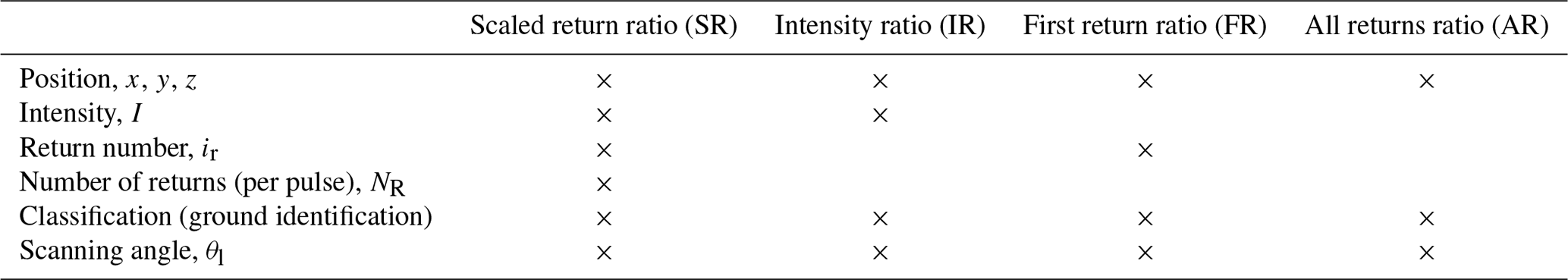
The SR method uses all of the standard recorded attributes of the reflections (Table 1) in the .las format, whereas the reference methods (in addition to zenith angle θ) use either only the position and classification (AR); the position, classification, and return number (FR); or the position, classification, and intensity (IR).

Table 1 Attributes used to calculate the PAD from ALSs with four different methods. The attributes are usually available with data in the .las format.

In the comparison with reference methods, we follow Solberg et al. (2006), Morsdorf et al. (2006), Richardson et al. (2009), and Boudreault et al. (2015) in assuming a spherical distribution of the reflecting surfaces of vegetation, corresponding to a value of μ=0.5, which is the equivalent of approximating that the effective forest density is the same looking from above, from the side, or from any other direction of the forest. While choosing a value of μ fitting for the vegetation of interest improves the PAI estimates (Yan et al., 2019), the focus of this study is the application of the Beer–Lambert law itself, and any change in μ would be common for the investigated methods; therefore, the value μ=0.5 has been kept throughout the study. To speed up the calculation, instead of using pulse-specific θ_l, we have used the average absolute angle within the grid box.

Recently, Vincent et al. (2017) presented a method in which intensity information is used to determine averaging weights specific to the return number, similar to the method presented here. However, the method proposed by Vincent et al. (2017) uses the intensity information averaged over the area of interest, whereas the method proposed in this paper uses individual intensity data for each pulse. If the individual intensities are not available in the data set or the data set is not ordered in consecutive returns, using the average data might be the only option. For a discussion on the implications of using average intensities as scales, please see Sect. 5.1.

3.2 Sites

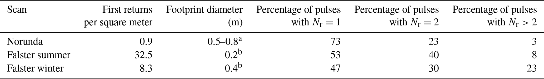
The methods were tested on three different data sets from two different sites: one site is a dense deciduous (beech) forest, scanned both with and without leaves; and the other one is a medium dense coniferous (mainly pine) forest. The data sets were chosen based on the fact that they cover two different and commonly occurring types of forests as well as the availability of both ALS data and ground-based PAI estimates. Table 2 shows a summary of scan characteristics for the three different data sets. The width of the laser beam at the ground differs from around 10 cm in the beech summer scan up to 80 cm in the coniferous forest, due to different instruments and flight altitudes. The scanning density also differs between sets (between less than 1 and more than 32 returns per square meter), providing contrasting conditions for testing the ALSs to PAD methods.

Table 2 Characteristics of the three ALS data sets used in the study. ^a Lantmäteriet (2016). ^b Personal communication with Laurids Rolighed J. Laursen, Niras (2017).

Dense beech forest: Tromnæs

This approximately 80-year-old forest of predominantly European beech (Fagus sylvatica L.) is located near the coast on the island of Falster in Denmark. During the leaf-on summer period, the canopy is very dense, whereas the wintertime tree structure is relatively open, as seen in Fig. 1. In order to accurately estimate the canopy height and density for the purpose of wind flow modeling, the forest was scanned during the summer time in 2013. The site was scanned again in a national survey in 2014 during the leaf-off winter period. In connection with a field campaign of wind observations upwind and downwind of the forest edge, the forest density was further measured using two LAI-2000 plant canopy analyzers (PCAs; LI-COR, Lincoln, NE, USA). The PAI was found to be approximately 1 and 6 m² m⁻² under leaf-off and leaf-on conditions, respectively. These measurements were performed using two instruments: one was placed well within the forest and the other, which was used for reference measurement, was placed well outside the forest. More information on the site can be found in Dellwik et al. (2014).

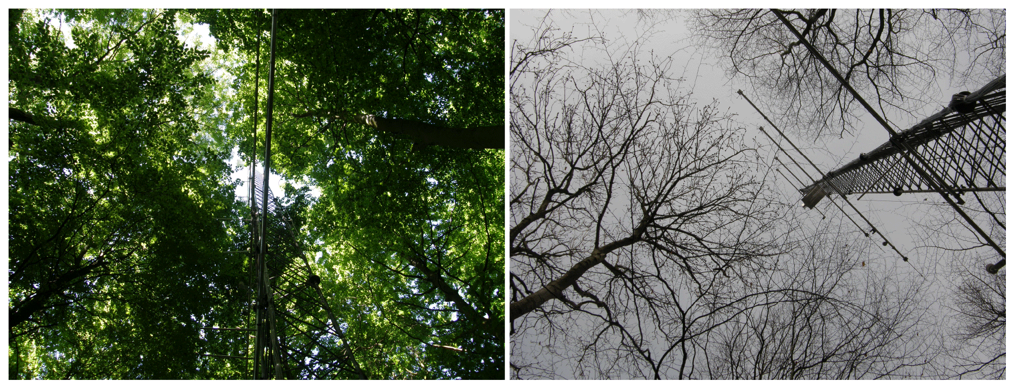
Figure 1 Photos taken at the position of the beech forest mast at the Falster site (Dellwik et al., 2014) illustrating the large difference between the summer (left) and winter (right) canopies.

From the point cloud of the two scans, we focus our analysis on a 300 m × 300 m tile which has its center coordinate at 54.7638^∘ N, 12.0396^∘ E. The respective data sets will be referred to as “Falster winter” and “Falster summer”.

Norunda

The Norunda site is a research site under the ICOS (Integrated Carbon Observation System) infrastructure, located in southeastern Sweden (60.0833^∘ N, 17.4833^∘ E). The forest cover is predominately Norway spruce (Picea abies) and Scots pine (Pinus sylvestris). A minor fraction (15 %) of deciduous trees, mainly birch (Betula sp.), is also present. The forest at the site is marked by its many clearings, characteristic of Swedish forest management. As part of the ICOS project, the forest density at the site has been analyzed with digital hemispheric photometry according to the ICOS protocol for ancillary vegetation measurements (Gielen et al., 2018). The site has also been scanned with an airborne laser as part of a national scan over Sweden (Lantmäteriet, 2016). The scan was carried out in November 2010, and the coverage is generally more than 0.5 ground reflections per square meter, although it is sometimes as low as around 5 ground reflections per 10 m × 10 m square in the densest parts of the forest. This data set will be referred to as “Norunda”.

Ground-based estimates of the forest were made in November 2018. Despite the difference of 8 years between the ground-based measurements and the airborne scan, the two data sets are expected to be comparable, as this particular forest stand was more than 100 years old and, thus, the growth rate was very low.

3.3 Evaluation parameters

3.3.1 Spatial differences

Spatial differences are demonstrated by showing differences in the PAI from the new method (SR) relative to the reference methods (IR, FR. and AR) for larger areas using a resolution of 10 m × 10 m for the three ALSs used. Calculation followed the same procedure for all methods, with the only distinction being the use of Eqs. (4), (5), (6), or (8) as a model for the extinction.

3.3.2 Comparison to ground-based methods

To provide an independent comparison, PAI from ALSs are compared to ground-based estimates. To mimic the footprint of the ground-based methods, reflections within a radius of one tree height from the center of the ground-based measurement were used. This yielded a circular binning area, as opposed to the square used in all other comparisons.

3.3.3 Sensitivity to ground albedo

In order to investigate the sensitivity to ground albedo, a test was constructed where the intensity values of returns classified as ground were manipulated. Ground intensity values were increased by 10 %, and the PAI was then calculated and compared to the PAI derived from the original data set. The same test was carried out again, but the ground intensity values were instead decreased by 10 %. The manipulation only affects SR and IR methods, as FR and AR exclude intensity information (Table 1). SR and IR showed only minor differences in sensitivity between a 10 % decrease and a 10 % increase in ground intensities; thus, the results are presented as sensitivity to a 10 % ground intensity alteration.

3.3.4 Sensitivity to grid size

All four ALS methods rely on the Beer–Lambert law which assumes a homogeneous spatial distribution of the scattering elements. This assumption is generally violated in forests, which have both a vertically and horizontally inhomogeneous distribution of scattering elements. With vertical binning in thin planes, the effect of vertical inhomogeneity is minimized, but heterogeneity in the horizontal direction is still present and results in a grid size sensitivity of the ALS to PAD methods. The reason for this can be illustrated by studying a single-layer PAI calculation for which the Beer–Lambert law simplifies to

$$\begin{array}{}\text{(9)}& \mathrm{PAI}=-{\displaystyle \frac{\cos {\mathit{\theta }}_{\mathrm{l}}}{\mathit{\mu }}}\ln \left({\displaystyle \frac{{\sum }_{\mathrm{ground}}{R}_i}{{\sum }_{\mathrm{all}}{R}_i}}\right)\end{array}$$

Calculating the PAI of an area by reducing the horizontal resolution so that there is only one single cell for the whole area is then proportional to $-\ln \left(\stackrel{\mathrm{‾}}{{\sum }_{\mathrm{ground}}{R}_i/{\sum }_{\mathrm{all}}{R}_i}\right)$, where the vertical bar represents the area average. Calculating the PAI for the whole area by taking the average of the PAI from a higher resolution is instead proportional to $-\stackrel{\mathrm{‾}}{\ln \left({\sum }_{\mathrm{ground}}{R}_i/{\sum }_{\mathrm{all}}{R}_i\right)}$. Because of the curvature of the convex logarithm function, Jensen's inequality states that $-\stackrel{\mathrm{‾}}{\ln \left({\sum }_{\mathrm{ground}}{R}_i/{\sum }_{\mathrm{all}}{R}_i\right)}>-\ln \left(\stackrel{\mathrm{‾}}{{\sum }_{\mathrm{ground}}{R}_i/{\sum }_{\mathrm{all}}{R}_i}\right)$, which means that sub-grid size variations in the ratio of the canopy to ground returns leads to lower PAI estimates for a larger grid size. The sensitivity of the routines to the grid size was investigated by simply calculating the PAD and PAI for the three data sets with a different horizontal resolution, ranging from 10 m × 10 m to 100 m × 100 m. Before calculating the PAI and PAD, the terrain height data were flattened in the vertical direction by subtracting the 10 m × 10 m ground height in order to avoid effects coming from terrain elevation changes within the grid cell.

4 Results

4.1 Spatial differences and comparison to ground-based methods

Maps of the calculated PAI can be seen in Figs. 2 and Figs. 3 and 4 for the Norunda and Falster sites, respectively. PAI magnitudes are shown for the SR method, and the differences of the IR, FR, and AR methods from the SR method are also given. It is immediately clear that forest characterization using ALSs has a big advantage over ground-based estimates due to the full horizontal coverage. In Fig. 2b, details of a road and clearings at the site shown in the aerial photo are also clearly visible in the PAI estimates. In terms of PAI magnitudes, FR gives the highest values for all three data sets (Figs. 2e, 3e, 4c), whereas the IR method shows the lowest values (Figs. 2d, 3d, 4b). Average PAI values over the area at the 10 m × 10 m resolution are given in the second column of Table 3; for Norunda, they show that the difference between the IR and SR methods is approximately 25 %, whereas it is less than or equal to 12 % for the AR and FR methods, respectively. In addition to these differences, larger local differences of up to approximately 100 % are visible in Fig. 2d–f. A comparison to the ground-based PAI observations is presented in Fig. 2c. Whereas the IR method shows a systematic underestimation relative to the ground-based observations, all other methods show an overestimation. These systematic differences could likely be removed by calibrating the extinction coefficient μ, as has been done in studies such as Solberg et al. (2009), but it is clear that such calibration would need to be method specific; therefore, it is not pursued further here. Another reason for an imperfect match is connected with the unknown footprint of the ground-based method (see Sect. 4.3 below).

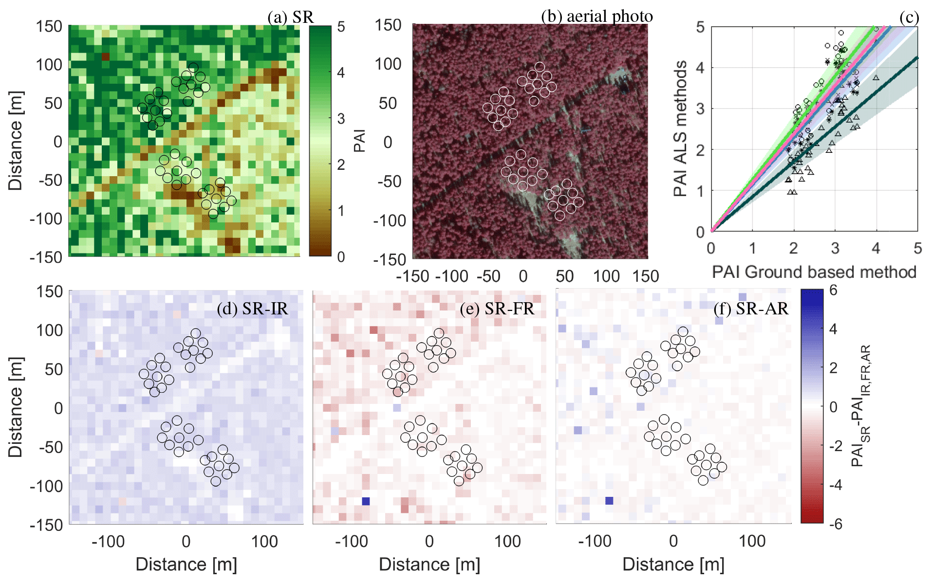
Figure 2 PAI evaluation at the Norunda site using a 10 m × 10 m grid: (a) the SR method; (b) an aerial photo (©Lantmäteriet) over the site, where the circles represent the placement of the ground-based observations; (c) a scatterplot of the hemispheric photo estimates and the ALS methods. The lines show linear regression forced through zero with shading indicating the 95 % confidence level (1.96 times the standard error). SR is represented using the blue line and stars, IR is represented using the dark green line and triangles, FR is represented using the bright green line and circles, and AR is represented using the pink line and crosses. Panels (d), (e), and (f) show the difference between SR and the IR, FR, and AR reference methods, respectively.

Whereas the results from SR, FR, and AR were relatively similar in Norunda, a larger difference is seen for these methods for the summer scan of the dense beech forest at the Falster site (Fig. 3). The SR method indicates large variability over the tile (Fig. 3a), with the PAI exceeding 10 m² m${}^{{}^{-}\mathrm{2}}$ in the lower-right and upper-left corners. A close look at the aerial photo (Fig. 3b) also indicates larger gaps in the forest in the lower left of the image, which could explain the relatively lower PAI in this area. Whereas the observed spatial variability using the SR method is similar for the IR method (Fig. 3d), it is strongly increased for the FR method (Fig. 3e) and decreased for the AR method (Fig. 3f). The very high PAI values using the FR method (Fig. 3e) can be explained by few pulses penetrating the dense upper canopy, which is in line with earlier observations on gap fraction versus beam footprint. The AR results are generally lower in magnitude than SR, whereas the FR results are of a higher magnitude. Averages over the whole tile (second column, Table 3) reveal mean differences of up to 30 % relative to the SR method.

The comparison between the ALS and ground-based observations (Fig. 3c) reveals a high degree of scatter and large standard errors. In addition to the potential reasons for the difference given above for the Norunda site, there is more uncertainty regarding the exact coordinates of the ground-based observations. In general, the ground-based observations seem to be saturated at around 6 m² m⁻², whereas the ALS data allow for a larger range.

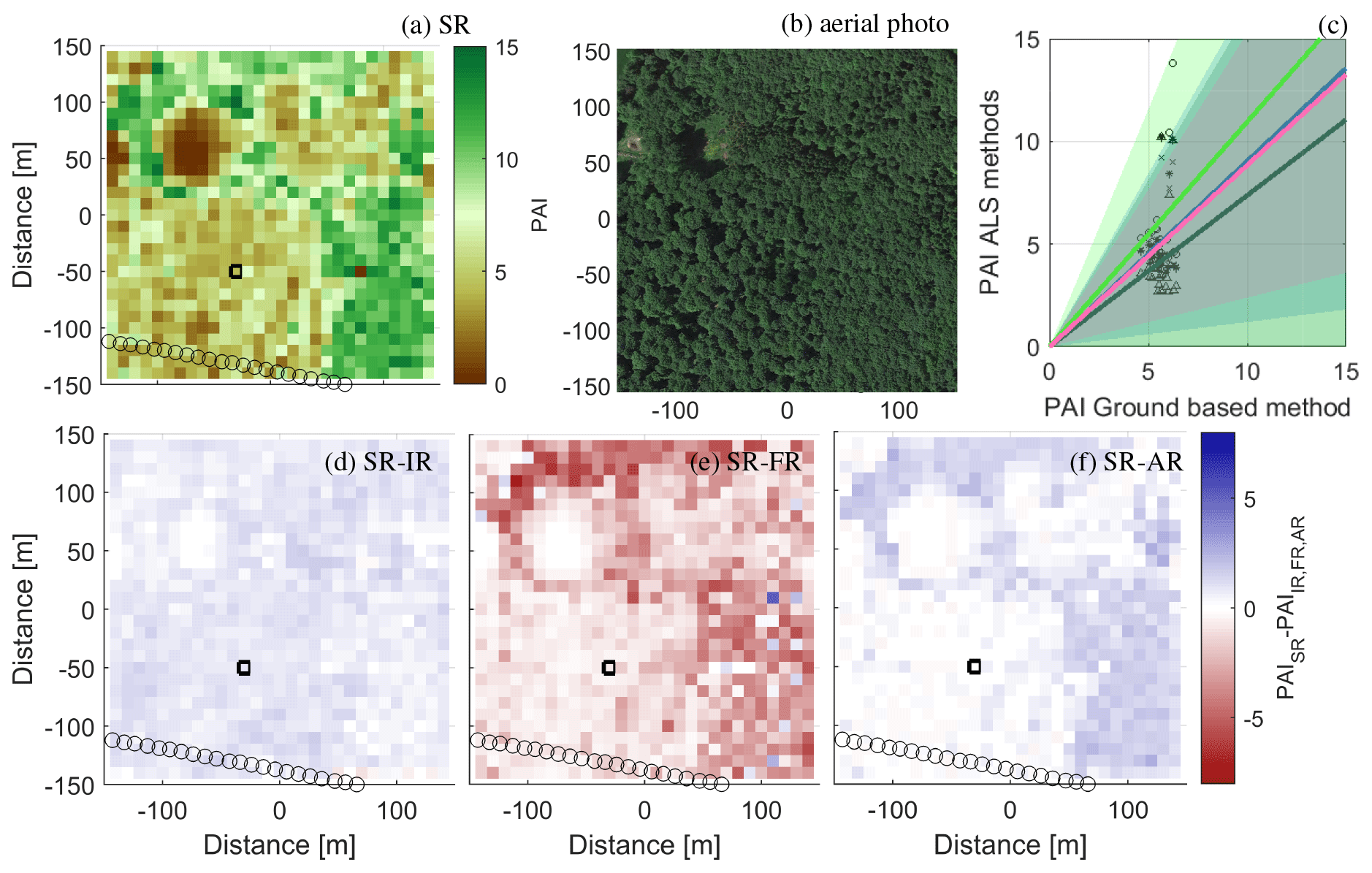
Figure 3 PAI estimates from the summer scan at the dense beech forest Falster site: (a) SR method; (b) an aerial photo (©Google Earth 2020) over the site; (c) a scatterplot of the ground-based estimates and the ALS methods. The lines show linear regression forced through zero with the shading indicating the 95 % confidence level (1.96 times the standard error). SR is represented using the blue line and stars, IR is represented using the dark green line and triangles, FR is represented using the bright green line and circles, and AR is represented using the pink line and crosses. The circles in the maps display the positions of the ground-based measurements. Panels (d), (e), and (f) show the difference between SR and the IR, FR, and AR reference methods, respectively. The black square marks the edges for the data used in Sect. 4.2.

Figure 4 shows the spatial variability over the same area as in Fig. 3 but for the winter scan of the site. Overall, the SR results indicate a low PAI (Fig. 3a), except for a small area to the right of the clearing, where values above 3 m² m⁻² are visible, corresponding to the location of a few coniferous trees. The IR method shows similar results to the SR (Fig. 3b), whereas much larger differences are observed for the FR and AR methods (Fig. 3c) and (Fig. 3d). The mean value over the whole tile (second column, Table 3 indicates differences of up to approximately 300 %. The reason for this is examined in detail in the next section, but (as can be seen from Fig. 1) even though the PAD of the upper canopy is low in winter compared with summer, there are relatively few gaps in the forest without any branches at all, effectively limiting the number of first-order returns reaching the ground.

Figure 4 PAI estimates from the Falster winter scan using various methods. (a) The PAI in a 10 m × 10 m square grid based on the SR method. Panels (b), (c), and (d) show the difference between SR and the IR, FR, and AR reference methods, respectively. The black square marks the edges for the data used in Sect. 4.2.

4.2 Single-grid-cell PAD and sensitivity to ground albedo

In order to illustrate how the ALS methods work, a grid cell encapsulating a single tree was selected. The location of the grid cell is highlighted in Figs. 3 and 4 using a black square. Figure 5 shows the reflections used and the resulting PAD for the four different methods. Figure 5a–e show the summer results, whereas Figure 5f–j show the winter results. The size of the markers in Fig. 5a–d and Fig. 5f–i indicates the weight that the algorithm gives to the reflections in the four different methods. As intensity is not regarded in the FR and AR methods, all markers in Fig. 5c, d, h, and i have the same size. As the SR method restricts the weight of the return, less difference in the marker size is seen in Fig. 5a and f, whereas more variability is seen for the IR method, where the reflections are not scaled. The first reflections are marked in blue, the second reflections are marked in red, and the third reflections are marked in black.

There is a marked difference between the lidar returns in the summer and winter scan. In summer (Fig. 5a–e), the majority of the returns come from the upper part of the foliage, predominately from first- and second-order returns of relatively high backscatter intensity. In winter (Fig. 5f–j), the intensity of the returns from the upper canopy is much lower, and the only returns with high intensity come from the stem and larger branches as well as from the ground.

The reason for the high PAI values in FR and AR relative to SR and IR in the case of Falster winter becomes apparent from Fig. 5. The ground returns used in the AR method are often higher-order returns, which are not included in FR. As seen in Fig. 1b, many of the gaps in the winter canopy are smaller than the ∼40 cm beam width for the Falster winter scan, making first-order returns in the lower canopy less likely. The data in Table 2 confirm that higher-order returns are more prevalent in Falster winter than in the other two scans. The AR method includes higher-order returns, but neither FR nor AR takes the low intensity in the returns from the upper canopy into account, ultimately leading to a relatively higher estimate of the PAD and PAI. Compared with the winter PAI reported in Dellwik et al. (2014) from ground-based observations, the average PAI was more than 4 times higher in FR (see Table 3) and more than 2 times higher in AR.

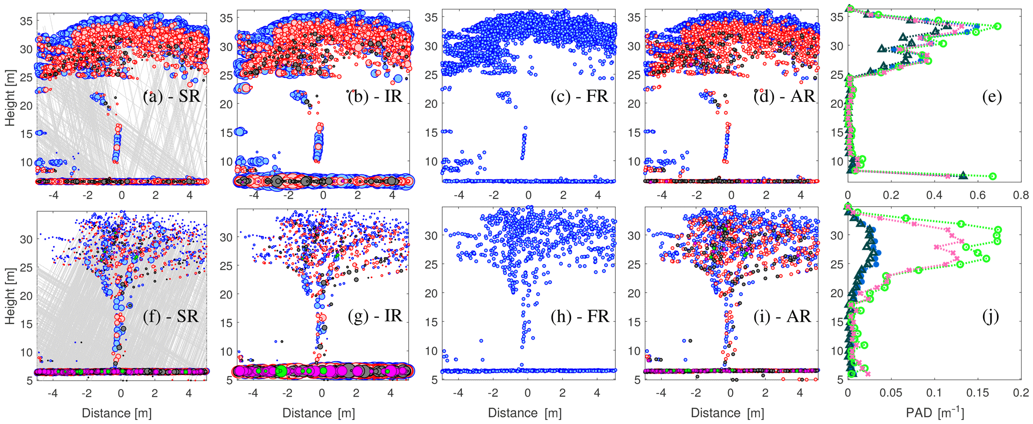
Figure 5 Backscatter reflections from within a 10 m × 10 m grid box taken from the Falster summer (a–e) and winter (f–j) scans. The color indicates the return number: first returns are represented using blue, second returns are represented using red, third returns are represented using black, fourth returns are represented using purple, and fifth returns are represented using green. The size of the marker indicates the weight of the return according to the four methods. The scaled return number for SR (a, f) is determined from Eq. (7); for IR (b, g), it is scaled by the medium intensity of the first-order canopy returns in the grid box; and for FR and AR (c, d, h, i), all returns are weighted the same. Note that the scale changes between the summer and winter. The gray lines indicate the path of the lidar beam between first- and higher-order returns; thus, lines are only shown for beams that have more than one return. Panels (e) and (j) shows the corresponding PAD for the summer and winter scan, respectively. SR is represented using blue stars, IR is represented using dark green triangles, FR is represented using bright green circles, and AR is represented using pink crosses. The location of the grid cell can be seen in Figs. 3 and 4.

The way first-order ground returns are treated in the methods that use the intensity of the backscatter (SR and IR) leads to a different sensitivity regarding the ground albedo. The difference in scaling technique between the SR and IR methods is visible in Fig. 5, particularly in the winter scan, through the dominance (large size) of the ground reflections in IR. As SR uses the scaling of each pulse, the intensity of a higher-order ground reflection is always smaller than that of a single first reflection, regardless of the actual back-scattered intensity.

The sensitivity to ground albedo was investigated by artificially changing the intensity values of the ground returns as detailed in Sect. 3.3. For the open pine forest of the Norunda site tile (Fig. 2), the mean difference in sensitivity was large, with SR only showing a 0.4 % change in the PAI for a 10 % change in the ground return intensity; the corresponding number for IR was 5.3 %. For the beech forest tile taken during the summer (Fig. 3), the sensitivity to a 10 % change in the ground return intensity was 0.8 % and 2.7 % for SR and IR, respectively. For the bare trees in winter, the corresponding values were 2.4 % and 6.0 % for SR and IR, respectively. The larger difference in Norunda comes from the larger share of first-order ground returns (see Table 2), owing to the more open structure of the forest. However, compared with the absolute differences between the methods, the albedo sensitivity is relatively small.

4.3 Sensitivity to grid size

As the canopy elements are heterogeneously distributed on all scales that are suitable for gridding when the PAD and PAI are calculated, the homogeneity assumption used when applying the Beer–Lambert law is violated. To illustrate the effect of that violation, the mapping of the PAI from ${\sum }_{\mathrm{ground}}{R}_i/{\sum }_{\mathrm{all}}{R}_i$ using Eq. (9) is shown in Fig. 6 in the x–y plane. Jensen's inequality is seen from the strong curvature of Eq. (9), which has the effect that an even distribution in ${\sum }_{\mathrm{ground}}{R}_i/{\sum }_{\mathrm{all}}{R}_i$ becomes positively skewed, with the long tail on the high PAI side. Lowering the resolution means narrowing the distribution of ${\sum }_{\mathrm{ground}}{R}_i/{\sum }_{\mathrm{all}}{R}_i$, thereby shortening the long tail more than the short tail in the PAI distribution and effectively lowering the PAI average.

Figure 6 The mapping of PAI from the ratio of ground returns to the total number of returns (${\sum }_{\mathrm{ground}}{R}_i/{\sum }_{\mathrm{all}}{R}_i$ at a 10 m × 10 m resolution) using Eq. (9) (black line in the x–y plane). The vertical axis shows the respective distributions of the PAI (y–z plane) and ${\sum }_{\mathrm{ground}}{R}_i/{\sum }_{\mathrm{all}}{R}_i$ (x–z plane), at a 10 m × 10 m resolution, for the four methods (SR is represented using blue, IR is represented using dark green, FR is represented using light green, and AR is represented using pink). The dashed lines indicate the area-averaged PAI from averaging the PAI at a 10 m × 10 m resolution for the Norunda (a), Falster summer (b), and Falster winter (c) scans.

Table 3 Values of the average PAI for the two sites, using different calculation methods and grid resolutions. ^∗ A number of PAD estimates were not possible due to fully attenuated first returns before ground level. The data were filled with PAD values of 0.1. Less than 1 % of the estimates were affected except for Falster summer at a resolution of 10 m × 10 m, where 4 % were affected.

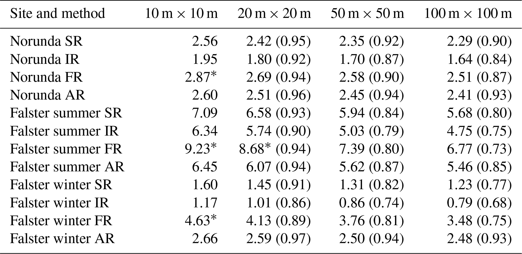
The sensitivity of the routines to grid size was investigated by evaluating the PAD and PAI for the three data sets using different horizontal resolutions ranging from 10 m × 10 m to 100 m × 100 m. Table 3 summarizes the sensitivity to grid size; it shows that for a magnitude change in grid size, the change in the PAI ranges from between a few percent to more than 30 % depending on the site and method. The AR method was found to be the least sensitive to grid size changes, followed by the SR method. The FR method was the most sensitive. The results indicate that IR and FR see more heterogeneity than the AR and SR methods. This is also observed in Fig. 6, where the distributions of ${\sum }_{\mathrm{ground}}{R}_i/{\sum }_{\mathrm{all}}{R}_i$ for IR are skewed towards high values (low PAI) and those for FR are skewed towards low values (high PAI). The observation in Sect. 4.1 that the AR method predicts less variation in PAI spatially, mainly due to underprediction in dense areas relative to the other routines, can also be seen in Fig. 6, particularly in Fig. 6c, Falster winter, where the distribution of ${\sum }_{\mathrm{ground}}{R}_i/{\sum }_{\mathrm{all}}{R}_i$ is much less skewed for AR than for the other methods. As also noted in Sect. 4.1, the SR method behaves in the same manner as the FR method in sparse regions and behaves like the IR method in dense regions, thus avoiding overprediction in the densest areas and underprediction in the least dense areas. As shown in Sect. 4.2, the weight of the first-order ground returns is limited in the SR method, while the reflectively of the ground leads to lower PAI estimates for IR, thereby widening the overall estimated PAI distribution.

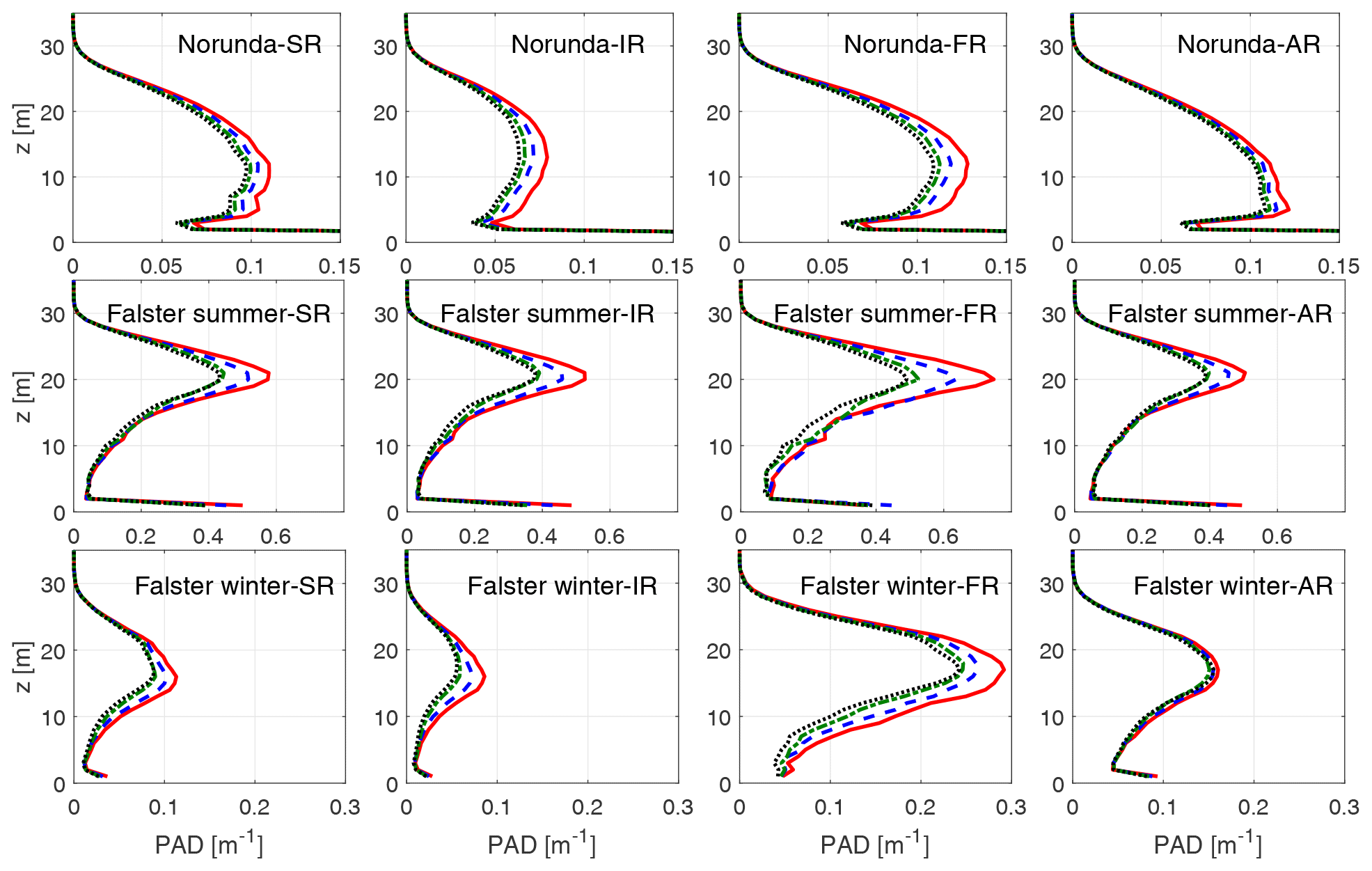
Figure 7 Average PAD profiles for the Norunda (top row), Falster summer (middle row) and Falster winter (bottom row) sites. The averages are based on a 10 m × 10 m (red full line), 20 m × 20 m (blue dashed line), 50 m × 50 m (green dash dotted line), and 100 m × 100 m (black dotted line) resolution using the SR, IR, FR, and AR methods (left to right), respectively.

The average PAD profiles for the three data sets using varying grid sizes are given in Fig. 7, where the data in Table 3, when split up into vertical profiles, reveal some differences between the methods. The difference in the PAD magnitude follow that of the PAI, with magnitudes particularly contrasting for Falster winter, although there are also some differences in the shape of the profile. In Norunda and Falster summer, the SR and AR methods appear very similar from Table 1 and Fig. 2a, d, and g as well as Falster summer (Fig. 3c). However, studying the PAD profiles, the SR method shows a less bottom-heavy profile, with a PAD maximum above a height of 10 m, in the canopy of most trees, whereas the AR method has the maximum PAD at around 5 m. For Falster summer, the difference between SR and AR is mainly in the dense regions (see Fig. 3a and d) which translates to a less pronounced upper-canopy peak in the average profiles in AR. In the Falster winter case, the profiles reveal a difference between the intensity-based SR and IR, with maximums at a lower height, and the FR and AR, which have maximums at higher heights. This is consistent with the case study in Sect. 4.2, in which a lack of intensity information regards the upper-canopy reflections with higher weight.

5 Discussion

5.1 Comparison between the ALS routines

In general, the methods resulted in similar spatial patterns and magnitudes of PAD. Systematic differences were, however, found for specific conditions. For winter (leafless conditions) the results showed differences between the area-averaged PAI of more than 400 %. Both FR and AR showed overpredictions relative to estimates in Dellwik et al. (2014); furthermore, values by FR and AR exceeded the maximum for beech trees reported in Bréda (2003). In addition, the ratio of winter to summer PAI was in excess of 0.4 for both FR and AR, which is also outside of the range reported in Bréda (2003). We attributed this to the high weights of reflections from the upper canopy, which is a result that follows from the lack of intensity information in connection with the tiny frontal area of branches to the footprint area of the lidar. The FR method further showed problems in the summer scan of the same forest, with a low number or lack of ground returns making the PAI estimates very high or impossible (argument in the logarithm of Eq. 3 becomes zero). This result indicates that using the intensity information provides a key benefit when the lidar footprint is large compared with common gap sizes in the forest. On the other hand, the results also show a sensitivity to ground albedo when the intensity information is used. This sensitivity was present in both the IR and SR methods, but the effect in SR was limited to between 7.5 % and 40 % of the sensitivity in IR. Overall, the scaling technique introduced in SR limits effects related to ground albedo and the footprint to gap size ratio, which indicates that it might be less sensitive to stand characteristics and scanning parameters such as flight height and scan density. The present study included needle and broadleaf trees for in-leaf and leafless conditions in addition to a dense helicopter scan with a small lidar footprint as well as sparse scans with a relatively larger footprint; however, future studies that systematically vary scan characteristics in different types of forests could help further quantify the differences between methods.

The method of Vincent et al. (2017) is similar to the method presented herein and, thus, potentially also has many of the advantages of the SR method. However, their use of weights based on the average intensity per return number and number of returns is a key difference from using the actual intensity fraction of the return within the pulse. In their study, Vincent et al. (2017) found that return number within the pulse and the total number of returns in the pulse described 51 % of the variance in intensity, which indicates that using average intensity numbers omits roughly half of the variation that is captured by using pulse-specific intensity information. For the data sets presented in this study, the average intensity roughly splits evenly among the returns in the two full-leaf scans; however the leafless scan was very different, as the average ground return was consistently more than twice as intense as any of the canopy returns, regardless of the number of returns. When we tested the difference between the SR method using individual and average weights, the absolute relative difference in the PAI estimates between the two was less than 5 % in the full-leaf scans; however, the difference was 25 % on average for the winter scan. Hence, if possible, the use of individual weights should be preferred, especially during the leafless state.

In cases of strong heterogeneity and focus on the actual PAD, as opposed to effective PAD, the method presented in Detto et al. (2015) provides an alternative to the approximation Beer–Lambert law, and future research in that direction is interesting, especially with increasing access to computational power.

5.2 The effects of resolution

How to optimally select resolution for PAI and/or PAD estimation by ALSs is still an open question. From Table 3, it is clear that a coarser resolution leads to a systematically lower PAI. The results agree with Boudreault et al. (2015), who presented a study on grid resolution using the FR algorithm in a spruce forest, varying the resolution from 5 m × 5 m to 30 m × 30 m. The results also agree with the analysis of Dufrêne and Bréda (1995), who presented a comparison between the leaf area index from litter collection and from ground-based PAI observations using the plant canopy analyzer (LI-2000, LI-COR Inc., Nevada), which is based on light penetration from five concentric rings. The PAI readings from the plant canopy analyzer systematically decreased in magnitude when rings at higher zenith angles were included in the estimate. The inclusion of more rings at high zenith angles can directly be translated to an enlargement of the measurement footprint, which makes the results from Dufrêne and Bréda (1995) comparable to the ALS-based results on gridding resolution from this study. As stated above, Jensen's inequality for convex functions explains these systematic changes. Hence, when estimating the PAI for heterogeneous forests from instruments that are based on the exponential decay of radiation into the canopy, the results can be expected to be resolution dependent. It should also be noted that results shown in Fig. 6 demonstrate that grid size sensitivity is dependent on the magnitude of PAD and/or PAI than less dense forests, and that this dependence enhances grid size sensitivity. Additionally, as discussed above, forest density in combination with the scan density (the number of returns per square meter) sets an upper limit for the possible resolution. Whereas the results in Table 3 show that systematic changes with resolution occurred for all four tested methods, there was significant variability between the tested methods, where FR always showed the highest sensitivity and AR and SR showed the lowest sensitivity.

The optimal resolution likely depends on the application. In wind modeling there is, for example, the optimal ratio of the resolution of the PAD field and flow field to consider, where the resolution of the flow field puts an upper limit on the resolution of the PAD field. Ivanell et al. (2018) concluded that for a predominantly forested area, where the drag force from the forest on the wind was modeled by means of PAD profiles, the value of the surface roughness below the canopy had very little impact on the flow above the forest. This implies that uncertainty in the lower part of the canopy is acceptable for wind modeling. Further research into how to optimally choose the grid resolution is needed.

6 Conclusion

We presented a new method to calculate the PAI and PAD from airborne laser scans (ALSs). This method uses all available reflection attributes commonly stored in the ALS data sets and combines benefits from earlier published algorithms. In order to evaluate the performance of the new method, it was used together with three reference methods on sites with contrasting characteristics. The results of the new routine showed no marked weakness with respect to sensitivity to forest characteristics, grid resolution, beam attenuation, and the ratio of ground to canopy returns, whereas all reference methods were challenged in one of those categories. In summary, the results indicate that the new algorithm is robust and would, therefore, perform well for a wider range of vegetation types than tested here.

The new routine is applicable provided that each data point in the data set contains information on the number of returns in the pulse and the return number of the specific point and that the data are ordered such that consecutive reflections from the same pulse are grouped in the data set. For the ALS data sets that we used in this study, these criteria have been fulfilled.

The results showed a dependence on the grid resolution of the derived PAI and PAD fields that was systematic for all methods. The grid sensitivity was linked to the violation of the homogeneity assumption in the Beer–Lambert law, which can also be explained by the Jensen's inequality for convex functions. The grid resolution sensitivity varies between the methods (from a 7 % to 32 % reduction in PAI for a magnitude change in grid size), where the new method showed the second-lowest sensitivity.

Despite the issues identified with airborne lidars for the determination of plant area and plant density, the similarities between the four tested methods highlight the prospect of obtaining PAD and PAI measurements with great spatial coverage, which are both precise and accurate, especially with regards to the uncertainty levels in established ground-based methods (Yan et al., 2019). The use of airborne lidar scans to derive maps of the PAD and PAI also provides a promising way to greatly reduce the subjectivity and likely uncertainty of any atmospheric modeling that involves air–canopy interactions, such as drag, heat transfer, and gas exchange.