the Creative Commons Attribution 4.0 License.
the Creative Commons Attribution 4.0 License.
 | 08 Dec 2020
Spatially resolved evaluation of Earth system models with satellite column-averaged CO2
Michael Buchwitz
Maximilian Reuter
Peter M. Cox
Pierre Friedlingstein
Veronika Eyring
Earth system models (ESMs) participating in the Coupled Model Intercomparison Project Phase 5 (CMIP5) showed large uncertainties in simulating atmospheric CO2 concentrations. We utilize the Earth System Model Evaluation Tool (ESMValTool) to evaluate emission-driven CMIP5 and CMIP6 simulations with satellite data of column-average CO2 mole fractions (XCO2). XCO2 time series show a large spread among the model ensembles both in CMIP5 and CMIP6. Compared to the satellite observations, the models have a bias of +25 to −20 ppmv in CMIP5 and +20 to −15 ppmv in CMIP6, with the multi-model mean biases at +10 and +2 ppmv, respectively. The derived mean atmospheric XCO2 growth rate (GR) of 2.0 ppmv yr−1 is overestimated by 0.4 ppmv yr−1 in CMIP5 and 0.3 ppmv yr−1 in CMIP6 for the multi-model mean, with a good reproduction of the interannual variability. All models capture the expected increase of the seasonal cycle amplitude (SCA) with increasing latitude, but most models underestimate the SCA. Any SCA derived from data with missing values can only be considered an “effective” SCA, as the missing values could occur at the peaks or troughs. The satellite data are a combined data product covering the period 2003–2014 based on the Scanning Imaging Absorption Spectrometer for Atmospheric Chartography (SCIAMACHY)/Envisat (2003–2012) and Thermal And Near infrared Sensor for carbon Observation Fourier transform spectrometer/Greenhouse Gases Observing Satellite (TANSO-FTS/GOSAT) (2009–2014) instruments. While the combined satellite product shows a strong negative trend of decreasing effective SCA with increasing XCO2 in the northern midlatitudes, both CMIP ensembles instead show a non-significant positive trend in the multi-model mean. The negative trend is reproduced by the models when sampling them as the observations, attributing it to sampling characteristics. Applying a mask of the mean data coverage of each satellite to the models, the effective SCA is higher for the SCIAMACHY/Envisat mask than when using the TANSO-FTS/GOSAT mask. This induces an artificial negative trend when using observational sampling over the full period, as SCIAMACHY/Envisat covers the early period until 2012, with TANSO-FTS/GOSAT measurements starting in 2009. Overall, the CMIP6 ensemble shows better agreement with the satellite data than the CMIP5 ensemble in all considered quantities (XCO2, GR, SCA and trend in SCA). This study shows that the availability of column-integral CO2 from satellite provides a promising new way to evaluate the performance of Earth system models on a global scale, complementing existing studies that are based on in situ measurements from single ground-based stations.
- Article
(19138 KB) - Full-text XML
- BibTeX
- EndNote


The Intergovernmental Panel on Climate Change (IPCC) Fifth Assessment Report (AR5) concluded that since 1950 many of the observed changes in the climate system have been unprecedented in the instrument record, confirming an unequivocal warming of the climate system (IPCC, 2013). Increasing emissions of greenhouse gases (GHGs) are the key drivers of anthropogenic climate change. The most important anthropogenic greenhouse gas is carbon dioxide (CO2), with CO2 emissions contributing more than half of the total global radiative forcing in 2011 relative to 1750 (IPCC, 2013). It is therefore important to monitor the long-term changes in atmospheric CO2 concentrations, to understand the sources and sinks of carbon and to provide reliable projections of future CO2 concentrations under various scenarios.
Photosynthesis causes a net uptake of atmospheric CO2 and thus declining atmospheric CO2 concentrations in the growing season. Conversely, atmospheric CO2 concentrations rise throughout the dormant season when there is a net release of CO2 from the land due to decomposition of organic matter in soils. This uptake and release of carbon by the terrestrial biosphere throughout the year causes a seasonal cycle of atmospheric CO2 (Keeling et al., 1989). The seasonal cycle amplitude (SCA) has been increasing over the last 50 years, with higher increases in higher latitudes (Barnes et al., 2016; Graven et al., 2013; Yin et al., 2018; Keeling et al., 1995; Keeling et al., 1996; Myneni et al., 1997; Piao et al., 2018). A number of studies have explored the effects of CO2 fertilization, land-use change and climate warming on the SCA (Bastos et al., 2019; Zhao et al., 2016; Fernández-Martínez et al., 2019). Although models do not agree unanimously, the dominant effects are a positive trend in SCA due to the CO2 fertilization combined with a negative trend due to climate warming. Some models, however, show a large positive trend due to climate warming (Zhao et al., 2016). Land use is found to be a weaker effect in comparison to CO2 fertilization and climate warming (Bastos et al., 2019; Fernández-Martínez et al., 2019).
Most long-term measurements of CO2 are from ground-based stations. In situ ground-based measurements at Mauna Loa (Hawaii, USA) started in 1958, providing the first evidence that fossil fuel combustion leads to a measurable increase in atmospheric CO2 concentrations (Keeling et al., 1976). Other observatories around the globe now also measure atmospheric CO2, reporting an increase of about 45 % since pre-industrial times (Ciais et al., 2013; Friedlingstein et al., 2019).
Satellite measurements of CO2, with first near-infrared/short-wave-infrared (NIR/SWIR) nadir-based (downward-looking) satellite retrievals starting in 2002, can complement the ground-based measurement network and provide regional and spatial distributions of CO2. The quantity obtained from measurements with NIR/SWIR satellite instruments is the column-average dry-air mole fraction of atmospheric CO2, denoted as XCO2. XCO2 is a dimensionless quantity defined as the vertical column of CO2 divided by the vertical column of dry air (i.e., all air molecules except water vapor) often given in ppmv (parts per million per volume). An analysis of growth rates (GRs) and SCA from satellite data and their sensitivity to growing season temperature anomaly presented in Schneising et al. (2014) shows a negative correlation between SCA and growing season temperature anomaly for the period 2003–2011, which was confirmed by Yin et al. (2018) for SCA anomaly in this timeframe. Satellite XCO2 products are often used in combination with atmospheric transport inverse modeling approaches to obtain information on surface fluxes by using a global or regional transport model with free fit parameters (Basu et al., 2013; Houweling et al., 2015; Reuter et al., 2014; Chevallier et al., 2014). The satellite data can also be used to constrain process parameters of a terrestrial biosphere model, e.g., as part of the Carbon Cycle Data Assimilation System (CCDAS; e.g., Kaminski et al., 2013), and have been used for the evaluation of chemistry–climate models (Hayman et al., 2014; Shindell et al., 2013). In the last few years, satellite data have also been used in direct comparison to output from climate models (e.g., Calle et al., 2019), characterizing rise and fall segments in seasonal cycles from GOSAT and comparing them to model output.
A large ensemble of climate model simulations for different type of experiments under common forcings is provided by the Coupled Model Intercomparison Project (CMIP), with output available for CMIP5 (Taylor et al., 2012) and more recently phase 6 (CMIP6; Eyring et al., 2016a). Earth system models (ESMs) produce a large range in projected atmospheric CO2, as a result of uncertainties in the future evolution of natural fluxes (Arora et al., 2013; Friedlingstein et al., 2006). Overall CMIP5 models overestimate the carbon content of the atmosphere (Friedlingstein et al., 2014; Hoffman et al., 2014). The largest uncertainties are associated with the response of the land carbon cycle to changes in climate and atmospheric CO2 (Friedlingstein et al., 2014; Hajima et al., 2014). The ability of ESMs to simulate the land and ocean contemporary carbon cycle has previously been investigated by Anav et al. (2013). They showed that most models were able to correctly reproduce the main climatic variables and their seasonal evolution but found weaknesses in reproducing specific biogeochemical fields, such as a general overestimation of leaf area index and photosynthesis. However, the magnitude of the global photosynthesis is not well constrained by observations, with estimates ranging between 112 and 169 PgC yr−1 (Ryu et al., 2019), and the dataset used by Anav et al. (2013) is on the lower end of this range. For CMIP6, Arora et al. (2020) analyzed simulations with a CO2 increase of 1 % per year to quantify the carbon–climate feedbacks. They found no significant change in behavior from CMIP5 to CMIP6 but lower absolute values for models which included a nitrogen cycle.
In this paper, we focus on evaluating the growth rate and the seasonal cycle amplitude of simulated CO2, converted to XCO2, from CMIP ESMs which performed emission-driven simulations with satellite observations in CMIP5 and CMIP6. The paper is structured as follows: the data products used in this study are introduced in Sect. 2. Section 3 describes the methods used, including the calculation of all derived quantities. A comparison between CO2 flask measurements and XCO2 measurements at different locations is given in Sect. 4. The evaluation of CMIP simulations with satellite data is presented in Sect. 5, divided into sections focusing on the models' ability to simulate XCO2 time series, growth rate and seasonal cycle amplitude. A summary and conclusion are given in Sect. 6.
2.1 Observational datasets
2.1.1 Satellite XCO2
We use the Observations for Model Intercomparisons Project (Obs4MIPs) version 3 (O4Mv3) XCO2 satellite data (Buchwitz et al., 2017a, 2018). Obs4MIPs hosts observationally based datasets which have been formatted according to the CMIP model output requirements (e.g., variable definitions, coordinates, frequencies) in order to facilitate an easier comparison between observations and models (Ferraro et al., 2015; Teixeira et al., 2014; Waliser et al., 2020). The satellite product used here is a gridded (level-3) monthly data product with a spatial resolution following the Obs4MIPs format, produced as part of the Copernicus Climate Change Service (C3S). The O4Mv3 product is retrieved from two satellite instruments: Scanning Imaging Absorption Spectrometer for Atmospheric Chartography/Envisat (Bovensmann et al., 1999; Burrows et al., 1995) and the Thermal And Near infrared Sensor for carbon Observation Fourier transform spectrometer/Greenhouse Gases Observing Satellite (TANSO-FTS/GOSAT) (Kuze et al., 2009).
This monthly mean XCO2 satellite dataset covers a 14-year time span (2003–2016). It is obtained by gridding the level-2 product (individual soundings) generated with the ensemble median algorithm (EMMA; Reuter et al., 2013), in this case EMMA version 3.0 (EMMAv3; Reuter et al., 2017). EMMA combines several different XCO2 level-2 satellite data products from SCIAMACHY/Envisat (2003–2012) and TANSO-FTS/GOSAT (2009–2016) and includes a bias correction to all products during overlap phases, resulting in a good agreement during the overlap period. This product was validated against Total Carbon Column Observing Network (TCCON; Wunch et al., 2011) ground-based observations of XCO2, revealing a +0.23 ppmv global bias, a relative accuracy (defined as standard deviation of the station-to-station biases) of 0.3 ppmv and a very good stability in terms of a linear bias trend (−0.02 ± 0.04 ppmv yr−1) (Buchwitz et al., 2017b). While the dataset ends in 2016, our evaluation only goes up to the year 2014 because the historical simulations for CMIP6 end in 2014 and scenarios from the emission-driven simulations that could be used to extend the runs are not yet available for all considered models.
The number of observations depends significantly on the location with most points over locations with low cloud cover, high surface reflectivity and (at least) moderate to high Sun elevation. Coverage over ocean is sparse as ocean retrievals are only included from GOSAT Sun-glint mode observations – outside of glint conditions, the reflectivity of water is very low in the NIR/SWIR spectral region. Figure 1 shows the mean monthly coverage of the dataset for 2003–2014. In Sect. 5, we will show that taking into account this sampling in the evaluation of ESMs is essential for a proper comparison.
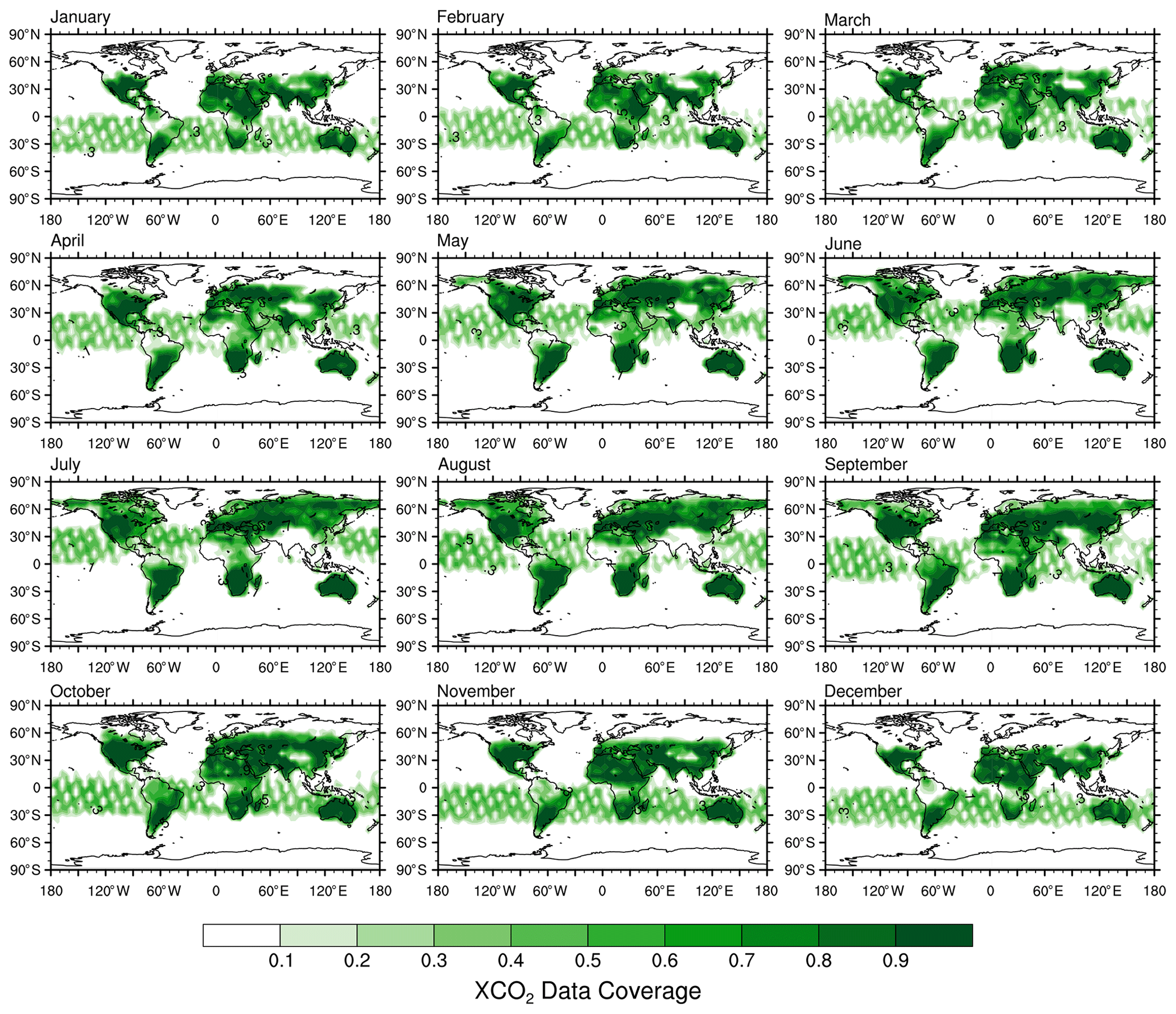
Figure 1Mean fractional coverage of monthly satellite data for 2003–2014. A value of 0 (white) signifies no available data, while a value of 1 (dark green) means that this grid cell contains data for all years of this month.
The dataset also contains uncertainty estimates for each grid cell, with a mean value of 0.92 ppmv, accounting for both statistical uncertainties from the individual soundings and uncertainties from potential regional and temporal biases (Buchwitz et al., 2017a). However, the overall uncertainties are small compared to inter-model differences (see Sect. 3.1) and are therefore neglected in our analysis.
2.1.2 Surface CO2 measurements
For the comparison of satellite XCO2 and surface CO2 data in Sect. 4, we have obtained surface flask measurements from the NOAA ESRL Carbon Cycle Cooperative Global Air Sampling Network (Dlugokencky et al., 2020). Measurement sites at locations with no available satellite data were excluded from the analysis, which ruled out the four baseline observatories in Mauna Loa and Samoa, as well as the South Pole and Point Barrow sites. Furthermore, sites which did not collect data during the period from 2003–2014 were discarded. From the remaining sites, a sample of five sites was chosen which had the best coverage of different latitudes, and when latitudes were similar, different longitudes were selected for increased spatial coverage. The selected sites are listed in Table 1.
Table 1List of active NOAA surface flask measurement sites used in this study.

2.2 Model simulations
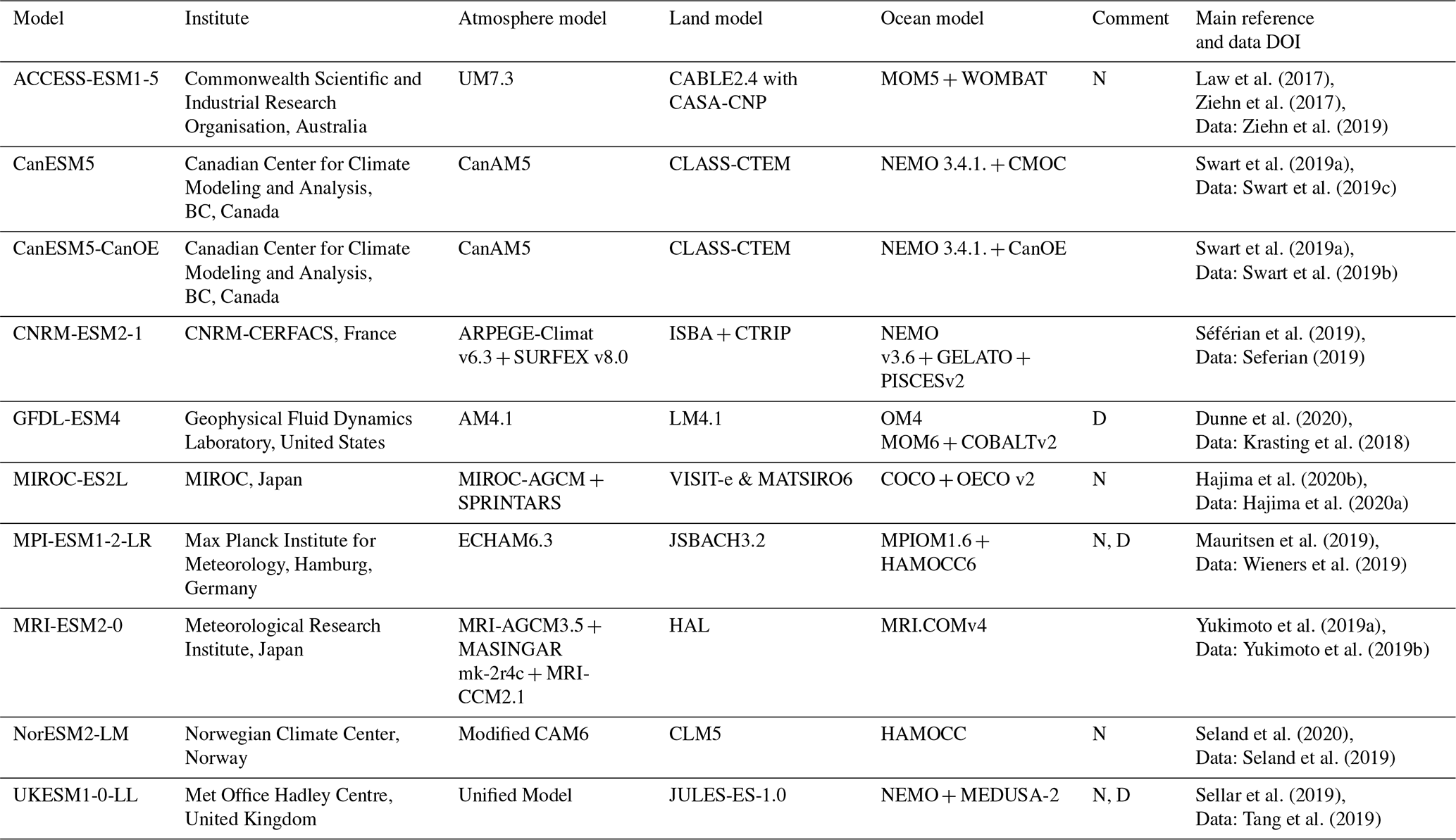
We use monthly mean output data from 10 CMIP5 and 10 CMIP6 models which performed emission-driven simulations, with three of the CMIP5 and five of the CMIP6 models including a nitrogen cycle. Tables 2 and 3 list all the CMIP5 and CMIP6 models used in this paper along with their atmosphere, land and ocean model component, respectively. Only models with an interactive carbon cycle are able to perform the emission-driven simulations, in which the emissions rather than the concentrations of the greenhouse gases are prescribed (Taylor et al., 2012; Eyring et al., 2016a). This allows the carbon cycle in the models to react to changes in climate and atmospheric CO2 by adjusting their carbon fluxes to the new climate conditions and providing the atmospheric CO2 concentration as an output (Friedlingstein et al., 2014). In order to facilitate the comparison between the satellite data and the CMIP5 emission-driven simulations, the historical simulations (1850–2005) were extended beyond 2005 with simulations from Representative Concentration Pathway (RCP) 8.5 (2006–2100), for which most ESM simulations are available. Since the period of observations only extends a decade beyond the historical runs, the choice of emissions scenario has a negligible impact on the results that we present below. For CMIP6, only the historical simulations are used, which end in 2014. For CMIP5, only one model had more than one ensemble member performing the emission-driven RCP8.5 simulation, and thus only one ensemble member for each model has been used. In CMIP6, several models have three or more ensemble members. We consider all of them in Fig. 3 for the time series to show the models' intrinsic variability but then proceed with the analysis with only the first ensemble member for each model. The different initial value ensemble members perform similarly to each other for the analysis presented in this paper, and using an ensemble mean would reduce the interannual variability found in each individual member.
Table 2CMIP5 models analyzed in this study. D stands for models including dynamic vegetation, and N stands for models including nitrogen cycles.
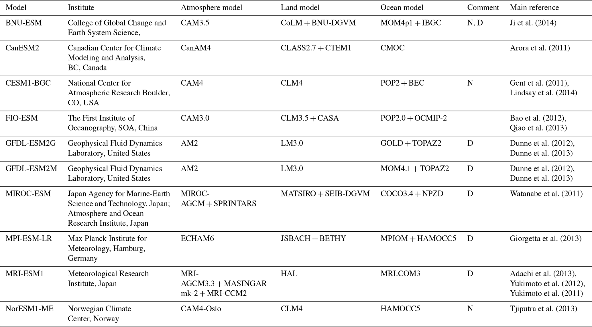
Table 3CMIP6 models analyzed in this study. D stands for models including dynamic vegetation, and N stands for models including nitrogen cycles.
3.1 Sampling of observations and models
For comparison of model and satellite data, first the CO2 data of the models were converted to XCO2 data. The model data were interpolated to the grid of the satellite dataset using a bilinear interpolation scheme and grid cells with missing values in the satellite data were also set to missing values in the model fields. Further sampling considerations are discussed in more detail in Sect. 5.3.2 and in Appendix B.
Most analysis is carried out with regional averages covering several grid cells. Unless specifically stated otherwise, these are calculated by taking the arithmetic averages over all grid cells weighted by their area for each month.
3.2 Calculation of growth rate, seasonal cycle amplitude and growing season temperature anomaly
We compute the GR following the method described in Buchwitz et al. (2018). Monthly resolved annual growth rates are calculated by subtracting the XCO2 value 6 months in the future from the one 6 months in the past. Then these monthly resolved growth rates are averaged to a yearly GR for a calendar year, and any year with less than 7 months of data is flagged as missing. The addition of the 7-month data availability was introduced to be consistent with the constraint on SCA as explained below.
We define the SCA as the peak-to-trough amplitude in a calendar year of the detrended time series. The time series is detrended with the cumulative sum of monthly growth rates, using the annual mean growth rates as substitution for missing values where necessary. The SCA is calculated by subtracting the minimum from the maximum value for each year with a minimum data availability of 7 months. When investigating the seasonal cycle of observationally sampled simulations at higher latitudes, the maximum value of the time series was generally only accounted for if more than 7 months of data were available. We therefore introduce the cutoff of 7-month data availability to preserve as many peaks as possible without restricting the data too much. However, as peak preservation cannot be guaranteed when any missing values are present, we can only speak of an effective SCA. The absolute SCA is not as important in our comparison, because we use the same sampling for both the model and observations.
The growing season temperature anomaly ΔT is calculated from the NASA Goddard Institute for Space Studies (GISS) Surface Temperature Analysis (GISTEMP) version 4 (Hansen et al., 2010) temperature anomaly map following Schneising et al. (2014). The data are masked to include only vegetated areas, using the MODIS land cover classification (Friedl et al., 2010a). Surface temperature anomalies are calculated with respect to their monthly climatologies. The data are averaged over the growing season if they cover only one hemisphere (April–September for the Northern Hemisphere; December to May for the Southern Hemisphere). Additionally, if the data cover both hemispheres, the whole year is taken into account. The growing season averages are taken because the temperature has a large influence on the plant growth and the resulting biospheric CO2 fluxes, which in turn drive both the SCA and interannual variability of the GR (Schneising et al., 2014).
3.3 Earth System Model Evaluation Tool (ESMValTool)
All figures in this paper were produced with the Earth System Model Evaluation Tool (ESMValTool) version 2.0 (v2.0) (Righi et al., 2020; Eyring et al., 2020; Lauer et al., 2020). Since its first release in 2016 (Eyring et al., 2016b), the ESMValTool has been further advanced, facilitating analysis of many different ESM components, providing well-documented source code and scientific background of implemented diagnostics and metrics, and allowing for traceability and reproducibility of results (provenance). ESMValTool v2.0 has been developed as a large community effort to specifically target the increased data volume of CMIP6 and the related challenges posed by analysis and evaluation of output from multiple high-resolution and complex ESMs. For this, the core functionalities have been completely rewritten in order to take advantage of state-of-the-art computational libraries and methods to allow for efficient and user-friendly data processing (Righi et al., 2020). Common operations on the input data such as regridding or computation of multi-model statistics are now centralized in a highly optimized preprocessor written in Python. ESMValTool v2.0 includes an extended set of large-scale diagnostics for quasi-operational and comprehensive evaluation of ESMs (Eyring et al., 2020), new diagnostics for extreme events, regional model and impact evaluation and analysis of ESMs (Weigel et al., 2020), as well as diagnostics for emergent constraints and analysis of future projections from ESMs (Lauer et al., 2020). For the study here, a new ESMValTool recipe has been developed that can be used to reproduce all plots of this paper.
Until recent years, most model–observation comparisons have been carried out using in situ surface CO2 data (e.g., Wenzel et al., 2016). As such, it is interesting to compare the differences between XCO2 and surface CO2 at different locations. Figure 2 shows a comparison of time series between both kinds of observations and the multi-model mean for both XCO2 and surface CO2 for CMIP6 (top) and CMIP5 (bottom) models. The multi-model mean for both XCO2 and surface CO2 is offset to have the same mean value as the satellite data, and this offset is noted above each time series panel. It is interesting to note that the offset appears to be larger at higher latitudes, thus showing a different latitudinal gradient between the models and the satellite data, indicating potential issues with surface fluxes or transport in the models. The multi-model mean and satellite data are averaged between all grid cells covering a radius around the stations, which results in a maximum of four grid cells to be considered. The mean and growth rate of XCO2 and surface CO2 are in very good agreement, while the multi-model mean overestimates both variables at all sites, with the overestimated mean XCO2 arising from the effect of higher growth rates over time. Furthermore, the offset from the modeled surface CO2 is higher than that of XCO2, while this difference is smaller for CMIP5. This might be due to the fact that the CMIP5 offset for multi-model mean XCO2 was larger overall with approximately 10 ppmv compared to the CMIP6 offset of approximately 2 ppmv.
SCA is higher at higher latitudes and also generally higher at the surface compared to the column average. This is to be expected as the processes dominating the seasonal cycle, respiration and photosynthesis, take place at the surface, leading to the higher SCA for station data and surface CO2 from models compared to the XCO2 values. Mixing of air coming from lower latitudes with lower SCA dampens the SCA in the column compared to surface SCA. This is evident in the increasing SCA difference between XCO2 and surface CO2 going from low-latitude to high-latitude stations, with no discernible seasonal cycle in the Southern Hemisphere due to the lack of land and vegetation. The multi-model mean follows this trend in the observations, although it underestimates the higher-latitude SCA, with a larger underestimation at the surface while capturing the XCO2 SCA relatively well. As this study aims at evaluating model simulations with satellite data, further analysis is restricted to XCO2.
5.1 XCO2 time series
The globally averaged time series of XCO2 is shown in Fig. 3 in the top panel, with CMIP6 (a) and CMIP5 (b) models sampled as the satellite observations (see Sect. 3.1). The observational uncertainty is too small to be seen in this plot and is therefore neglected. The middle panel shows the monthly resolved annual growth rate and the bottom panel the detrended seasonal cycle. All available ensemble members for CMIP6 models are used to show their internal variability. All ensemble members perform similar to one another. The multi-model mean is computed using the first ensemble member, which is also used in the further analysis. As in Fig. 2, an increase of XCO2 with time and a pronounced seasonal cycle for all models can be seen. The focus here is on the absolute values, as the trend (GR) and SCA are discussed in dedicated sections below. The CMIP6 models display a large range of absolute XCO2 values, ranging from an underestimation by 15 ppmv (MRI-ESM2.0 and MIROC-ES2L) to an overestimation by 20 ppmv (GFDL-ESM4). The model closest to the observations is CNRM-ESM2-1, which reproduces the mean value well, with the next closest models being NorESM2-LM and MPI-ESM1.2-LR, both overestimating XCO2 by about 5 ppmv. The multi-model mean shows an overestimation by approximately 2 ppmv or equivalently a time shift of 1 year. While the spread in the models has not decreased much since CMIP5, the overestimation of the multi-model mean has decreased from 10 to 2 ppmv. Furthermore, CMIP6 models which have predecessors in CMIP5 show similar biases as their predecessors, besides the MIROC models, which overestimated the mean by 15 ppmv in CMIP5 and underestimates it by that much in CMIP6. Both MRI models underestimate XCO2 significantly, while GFDL-ESM4 overestimates the atmospheric content even more. The MRI-ESM1 model was the only model in CMIP5 to underestimate XCO2 with respect to the observations, and this was by about 20 ppmv. This model underestimates the historical warming, causing plant and soil respiration to be too low, which leads to a larger land sink and a reduced atmospheric CO2 concentration (Adachi et al., 2013). This underestimation has been reduced by about 5 ppmv in CMIP6. The GFDL models show an overestimation of about 15 ppmv in both ensembles, and both CanESM models are 10 ppmv too high. A minor improvement can be seen for NorESM-LM over NorESM1-ME, with a decrease of the overestimation from 15 to 10 ppmv.

Figure 2Comparison of time series from satellite XCO2 (black), multi-model mean XCO2 (orange) and surface CO2 (red), and NOAA surface CO2 station data (blue) at selected sites, with the coordinates noted in brackets above the time series and the altitudes shown in the map plot (see Table 1). The multi-model mean for both XCO2 and surface CO2 was offset to have the same average value as the satellite XCO2 for better comparison, and this offset is noted above each time series. CMIP6 and CMIP5 multi-model means are shown in the top (a) and bottom (b) panels, respectively.
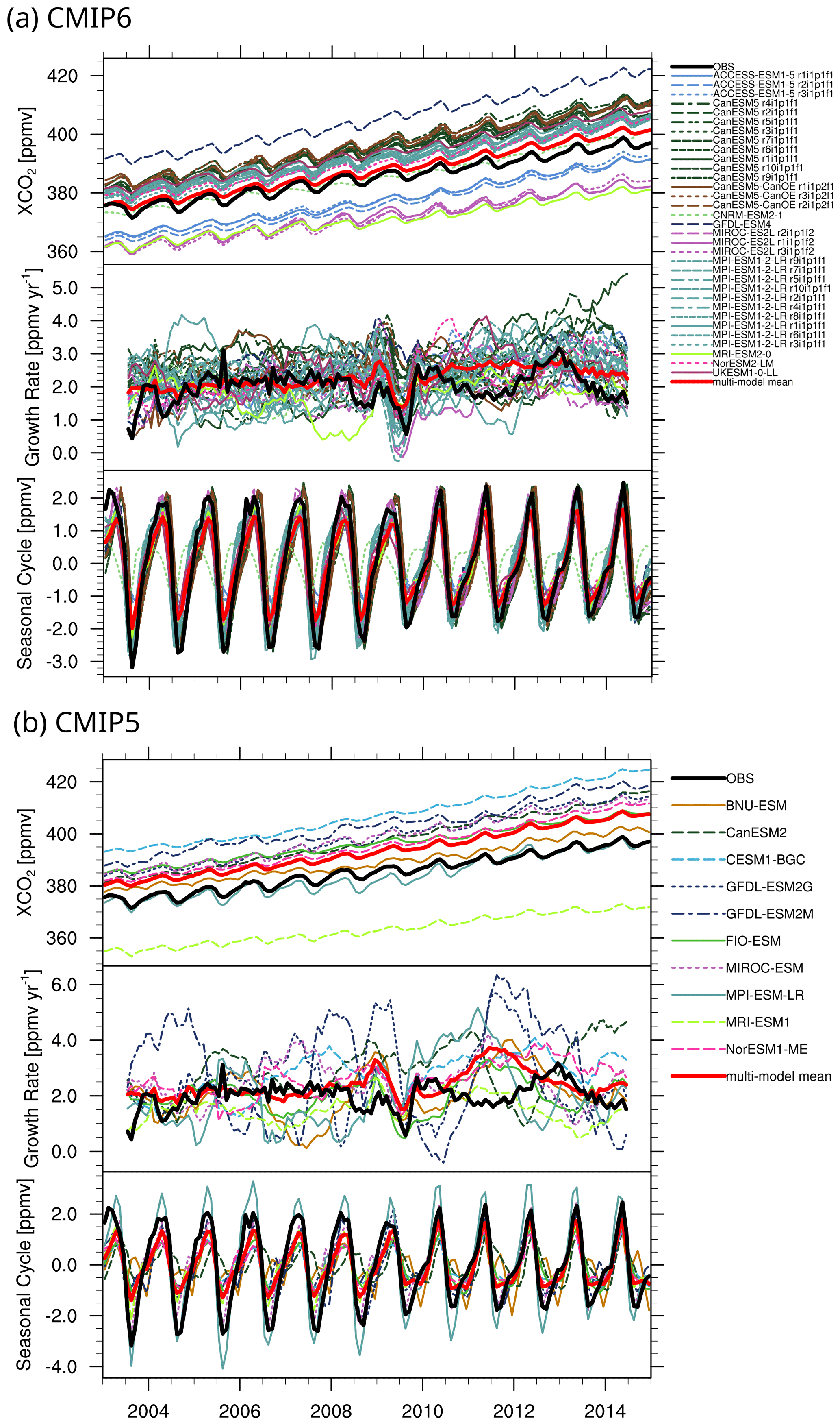
Figure 3(a) Global time series of monthly mean column-averaged carbon dioxide (XCO2) from 2003 to 2014 for the emission-driven CMIP6 model simulations in comparison to satellite XCO2 data (bold black line). The model output is sampled as the satellite data. The top panels show the time series, while the middle panels show the computed monthly growth rate, which has been used to detrend the data to obtain the seasonal cycle shown in the bottom panel. All available ensemble members for each model are shown to demonstrate the intrinsic variability of the models. (b) Same as Fig. 3a but for CMIP5. Only one ensemble member is shown.
5.2 Growth rate
The middle panel of Fig. 3 shows that while models capture the interannual variability of the growth rate quite well, they overestimate the mean growth rate compared to the observations. The correlation coefficient for the multi-model mean is at 0.48 in CMIP6 and 0.07 in CMIP5 which shows a large improvement in this area. The pronounced feature in 2009 is due to the introduction of the GOSAT data which changed the shape of the seasonal cycle and thus due to its calculation the monthly resolved annual growth rate. Fortunately, this feature gets averaged out when computing the annual growth rate and does not tangibly affect our conclusions. Figure 4 shows the global mean GR of XCO2 for 2003–2014 and its standard deviation over all years depicted as error bars, with the observations shown in black and the multi-model mean in red. The annual mean GR of the satellite data is 1.9 ± 0.4 ppmv yr−1, while the CMIP5 models (right) range from 1.5 ± 0.4 (MRI-ESM1) to 3.0 ± 0.9 ppmv yr−1 (CanESM2) with a multi-model mean of 2.4 ± 0.4 ppmv yr−1. In CMIP6 (left), the multi-model mean is slightly lower at 2.3 ± 0.3 ppmv yr−1, and the spread has decreased by 0.6 ppmv yr−1, with a range from 1.7 ± 0.4 (MRI-ESM2.0) to 2.6 ± 0.7 ppmv yr−1 (GFDL-ESM4). As expected from Fig. 3, the models – with the exception of MRI-ESM1, MRI-ESM2.0 and MIROC-ES2L – overestimate the growth rate, leading to an increased XCO2 level in the present-day atmosphere compared to observations. The interannual variability of the growth rate for the models is generally higher than that of the observations but well reproduced in the multi-model mean.
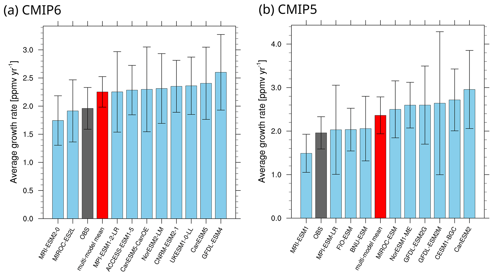
Figure 4Global mean and standard deviation over all years of annual growth rate of XCO2 during 2003–2014 for CMIP6 models (a) and CMIP5 models (b). The black bar represents the satellite observations, while the red bar depicts the multi-model mean.
Emergent constraints are relationships defined using an ensemble of models, between a measurable aspect of current or past climate and an aspect of Earth system feedback in the future, which can be constrained using observational data (Eyring et al., 2019). In Appendix C, we have tried to reproduce the trend in interannual variability (IAV) of CO2 growth rate to IAV of tropical temperature used by Cox et al. (2013) to develop an emergent constraint on the sensitivity of tropical land carbon to climate change but were unable to find a significant trend for this much shorter satellite-derived time series.
The spatial variability of the GR is small, as CO2 is long lived and well mixed in the atmosphere with a 1-year mean interhemispheric crossing time. Thus, there should be no significant regional changes on an annual level. Buchwitz et al. (2018) found the growth rate of the satellite dataset to be in agreement with those quoted by NOAA ESRL's global and Mauna Loa time series, as well as robust over several latitude bands. Our own analysis also shows only very small regional differences in the growth rate (not shown). No significant changes to the annual growth rates due to the satellite spatial coverage were found.
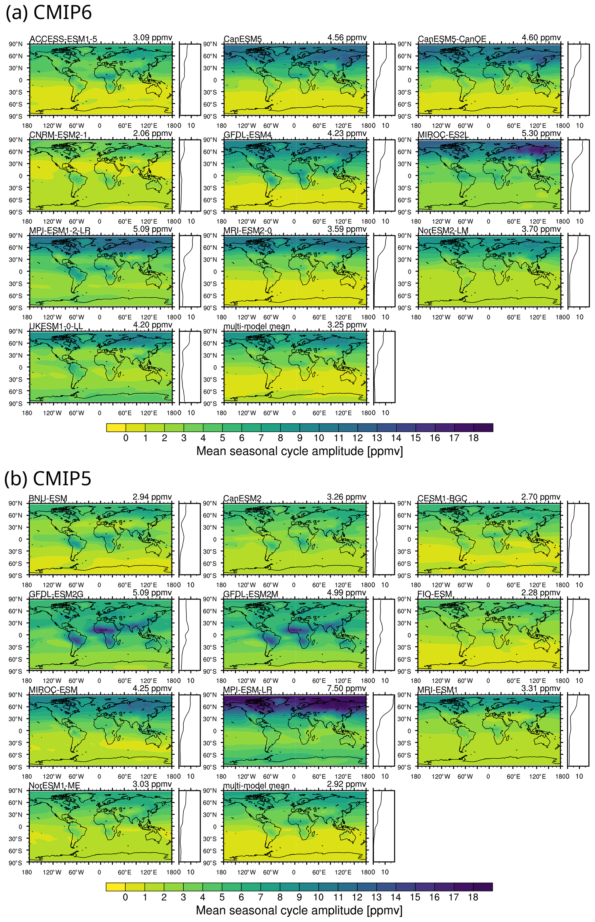
Figure 5Maps of mean annual seasonal cycle amplitude for 2003–2014 for the CMIP6 (a) and CMIP5 (b) models. The model name is given in the top left of each panel, and the top right shows the global average of the mean annual seasonal cycle. The panel to the right of the maps shows the same zonal mean SCA.
5.3 Seasonal cycle amplitude
This section about the SCA is divided into two subsections, with the first one taking a closer look at inter-model differences, while the second subsection is devoted to the impact of observational sampling.
5.3.1 Model differences
The lower panel in Fig. 3 shows the detrended global seasonal cycle for all models. Models in CMIP6 (a) show a strong improvement in their ability to capture both the seasonal cycle amplitude, as well as its phase compared to CMIP5 (b) but still underestimate the SCA. The correlation coefficient to the observed seasonal cycle is 0.93 in CMIP5 and 0.98 in CMIP6 for the multi-model mean. The only model in CMIP6 to significantly underestimate the seasonal cycle amplitude is CNRM-ESM2-1. Two errors have been identified causing this dampened seasonal cycle: ocean carbon fluxes are lagged in time, and in the emission-driven simulations, CO2 is considered as an active tracer and coupled with atmospheric chemistry. These chemical fields are restored to global mean climatological concentrations at the model surface, acting as a damping component to the CO2 concentrations (Séférian et al., 2019). Figure 5 shows maps of the climatological mean SCA (2003–2014) for all models, with the global mean given in the top right and the zonal averages shown in the panel attached to the right of the maps. All CMIP6 models (Fig. 5a) underestimate the SCA compared to satellite observations (Fig. 6, middle) in the global mean, with the closest mean SCA being MIROC-ES2L. This underestimation was already present in CMIP5 (Fig. 5b), with several studies discussing it for surface CO2 SCA (Wenzel et al., 2016; Graven et al., 2013). In CMIP6, the multi-model mean has a globally averaged mean SCA of 3.25 ppmv, compared to 2.92 ppmv for CMIP5, while the observations show an effective SCA of 5.89 ppmv (Fig. 6).
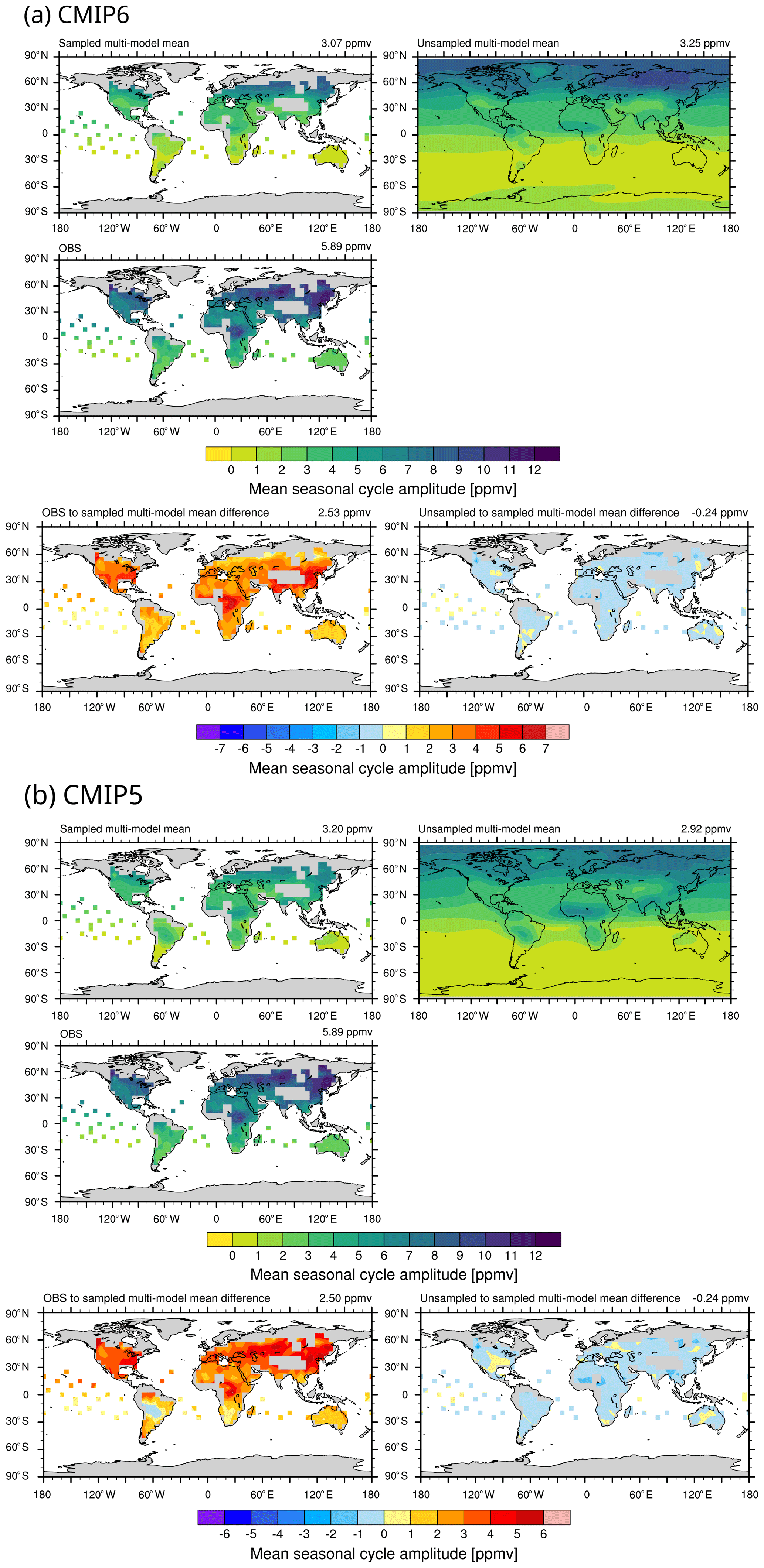
Figure 6(b) Same as Fig. 6a but for the CMIP5 multi-model mean.
Both models and observations show the well-known increasing SCA with increasing latitude, due to the more pronounced seasonal cycle of the climate at higher latitudes. Most models show a decreased growth from 0 to 30∘ N, with higher SCA increases in the lower tropics and northern midlatitudes. Overall, the zonal distribution is quite similar throughout the models, with UK-ESM1-0-LL showing increased SCA at 30–90∘ S. Tropical land regions in northern South America, Africa and southeast Asia show increased SCA values compared to the ocean SCA at this latitude for the same model. While in the GFDL CMIP5 models this was so pronounced that these regions showed a higher SCA than the higher latitudes (Dunne et al., 2013), this is no longer the case for GFDL-ESM4 in CMIP6. Dunne et al. (2013) attributed the GFDL problem in CMIP5 to the seasonality of respiration in the northern latitudes and an Amazonian low-precipitation bias which reversed the seasonal cycle synchronizing it with the African and Oceanian rain forests. The improvement in CMIP6 is due to a reduced ocean–atmosphere CO2 flux in the Southern Hemisphere, as well as the reduction of the high tropical land–atmosphere fluxes expressed over the ocean (Dunne et al., 2020).
The SCA in the CMIP5 MPI-ESM-LR model is on average twice as large as the observed one. The high SCA has been discussed in Giorgetta et al. (2013), where it was attributed to a combination of an overestimation of net primary productivity in ocean and land biology and uncertainties in atmospheric tracer transport. A particularly severe overestimation was seen in the Southern Hemisphere when comparing to station data. As shown in Fig. 6, we additionally find a large overestimation in XCO2 SCA in the Northern Hemisphere, in particular in the extratropics. For the CMIP6 successor model, MPI-ESM1.2-LR, the SCA is still the highest of the model ensemble but is no longer twice as high as the other models. However, it now shows a more pronounced SCA over the tropical land regions mentioned above, which was not as dominant in CMIP5.
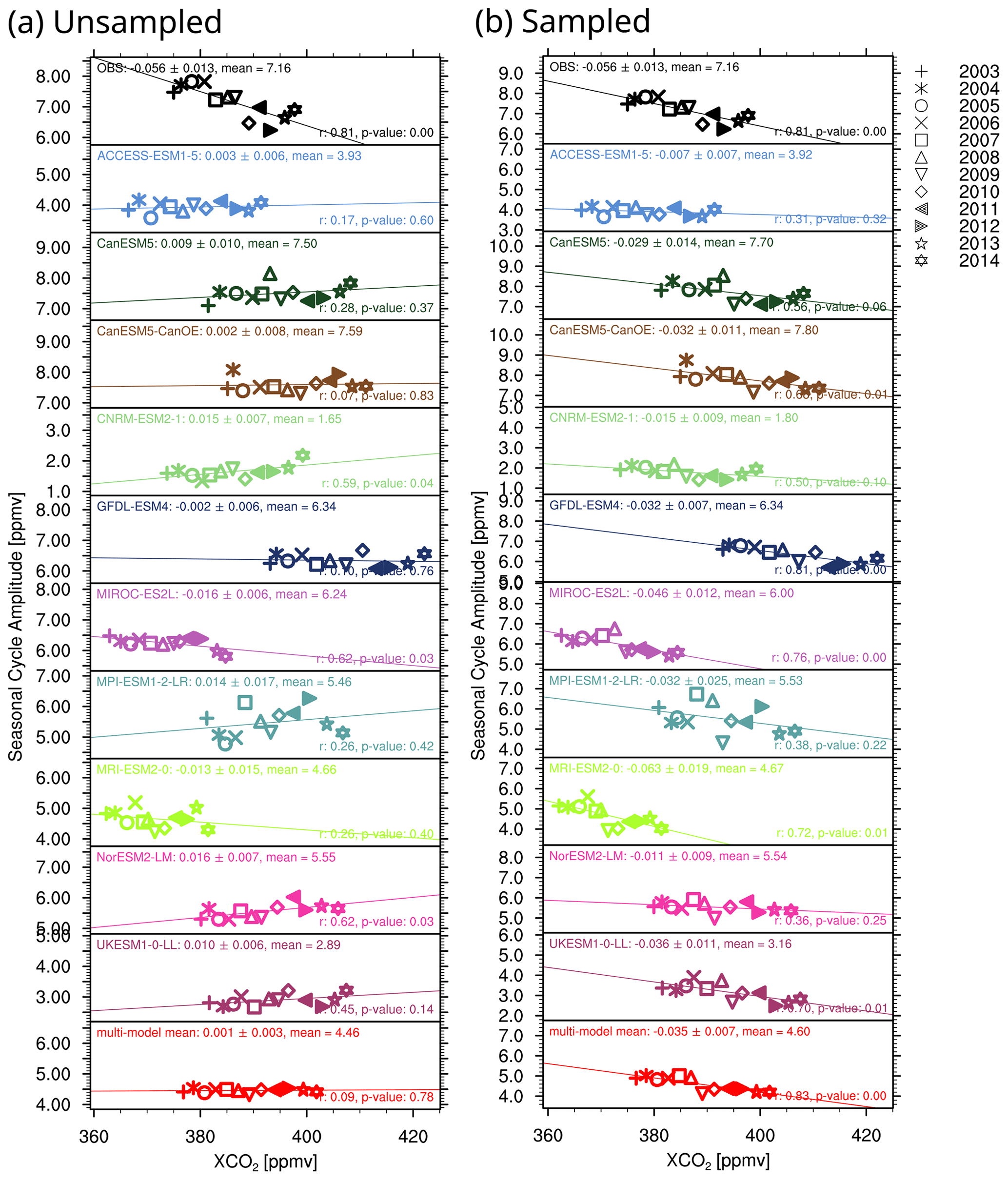
Figure 7Trend of SCA with XCO2 for 2003–2014 for the northern midlatitudes (30–60∘ N), including a linear regression with slope and mean SCA given in the top left of each panel and the Pearson correlation coefficient as well as the p value in the bottom right. Symbols denote the different years and model colors are consistent with previous figures. The left panels (a) show unsampled CMIP6 models, while CMIP6 models sampled according to the satellite data are shown on the right (b). Note that the y-axis range for each plot is the same and only differs by a shift.
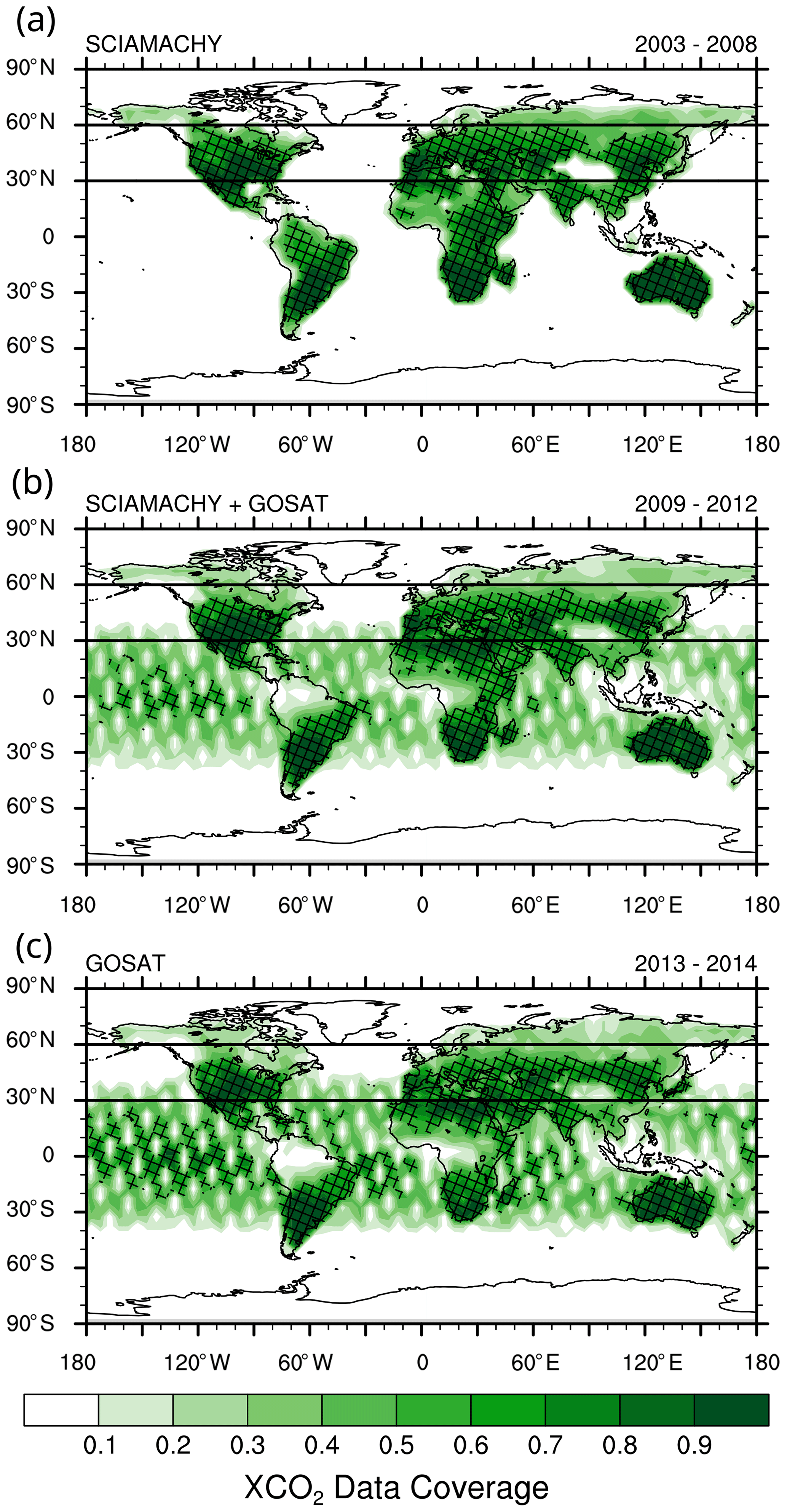
Figure 8Data coverage of the satellite observations for (a) 2003–2008 containing only SCIAMACHY data, (b) 2009–2012 containing the overlap of SCIAMACHY and GOSAT data and (c) 2013–2014 containing only GOSAT data. The patterned area highlights values above 0.5.
It is known that nitrogen limitations tend to suppress CO2 fertilization (Reich et al., 2006). Of the four models with the lowest overall SCA in CMIP5 (CESM1-BGC, FIO-ESM, NorESM1-ME and BNU-ESM), three of them – BNU-ESM, CESM1-BGC and NorESM1-ME – include a nitrogen cycle. The SCAs of NorESM1-ME and CESM1-BGC are very similar, which can be attributed to sharing the same land model (CLM4). FIO-ESM uses the predecessor CLM3.5 and is also comparable to the other two models. It was found that CLM4 had an unrealistically strong nitrogen limitation, which has been reduced in CLM5 (Wieder et al., 2019). In CMIP6, ACCESS-ESM1.5, MPI-ESM1.2-LR, MIROC-ES2L, NorESM2-LM and UKESM1.0-LL include a nitrogen model but none of them share the same land model. While ACCESS-ESM1.5 has the second lowest overall SCA, MPI-ESM1.2-LR and MIROC-ES2L have the highest, and thus the observation from CMIP5 models that N-cycle models feature a lower SCA no longer stands for CMIP6.
5.3.2 Influence of sampling
There are a number of ways to compare model SCA to observational SCA, beginning with a grid box comparison. Figure 6 shows a comparison of the multi-model mean of CMIP6 (Fig. 6a) and CMIP5 (Fig. 6b) to observations. The top right shows the unsampled SCA. The top left panel shows the effective SCA when using observational sampling and the middle panel the satellite data's effective SCA. All numbers are given in ppmv. For an easier comparison, the bottom panels show the absolute difference plots, with the left panel depicting the difference between sampled model and observations, and the right panel the difference between the sampled and unsampled model. Observational sampling slightly lowers the SCA, which is to be expected, as it could lead to masking out the peaks or troughs. While this effect was minimized by imposing the restriction of only computing the SCA of a year when at least 7 months of data are available, it is still a possibility. We therefore classify this SCA as an “effective SCA”. However, the SCA does not seem to decrease significantly through sampling and the difference does not follow a trend in latitude, so a grid box comparison seems feasible. This paves the way for more comprehensive spatial investigations, which previously relied on data from ground-based stations with sparse spatial coverage. While the stations provide data in higher latitudes that the satellite dataset does not cover, in the tropics and midlatitudes the spatial coverage of the satellite is superior to the ground-based stations. A downside with this approach is the sparsity of the data when using observational sampling. Furthermore, this becomes a computationally expensive operation, as the SCA will need to be calculated for each grid box.
Another approach often used in model analysis is area averaging, e.g., over different latitude bands like the tropics or the northern midlatitudes. Using surface flask measurements, Wenzel et al. (2016) found an increased SCA with rising CO2 concentration for CMIP5 using model data from the full historical simulation (1850–2005) – CO2 fertilization – and used this to establish an emergent constraint on the fertilization of terrestrial gross primary productivity (GPP). Figure 7 shows the SCA trend of CMIP6 models versus XCO2 for 2003–2014 in the northern midlatitudes (30–60∘ N), including a linear regression including slope, mean SCA, Pearson correlation coefficient and p value. The left panel shows the trend in the unsampled models, while the right one shows the trend when following the sampling of the satellite data. The SCA was computed after a weighted area average was determined on the XCO2 time series. While some of the unsampled models show an increasing SCA trend with increasing XCO2, which is in agreement with the findings from Wenzel et al. (2016), others do not show a statistically significant trend and the multi-model mean shows an insignificant positive trend. The sampled model data (right) show a significant negative trend. Calculating the average with a zonal average before summing up the latitude bands does not change this result.
To investigate this change in trend due to observational sampling, Fig. 8 shows the data coverage for different time periods, 2003–2008 for SCIAMACHY only measurements (top), the overlap between the two satellites in 2009–2012 (middle) and 2013–2014 for the GOSAT satellite only (bottom), with the pattern marking areas with a coverage of 50 % or above. Above 50∘ N, SCIAMACHY measurements include more areas with 50 % or more coverage compared to GOSAT measurements. With a larger SCA in higher latitudes, it implies that SCIAMACHY would have a larger average SCA over this region compared to GOSAT, hence artificially generating a decreasing trend in the observed SCA, when moving from SCIAMACHY to GOSAT. Figure 9 shows the CMIP6 effective SCA trend with XCO2 using SCIAMACHY and GOSAT masks obtained from masking out points with less than 50 % coverage. While the slopes remain largely the same, the mean effective SCA is higher in the models using the SCIAMACHY mask than when using the GOSAT mask. This mean SCA difference is larger than the total SCA difference within a model using the same sampling for the whole time period. Thus, when considering the observational time series and its full sampling, the trend intrinsic to the model is dominated by the negative SCA difference going from the SCIAMACHY to the GOSAT data coverage and thus changed to the negative trend seen in the observations. We can therefore attribute at least part of the negative trend in the satellite data to the different data coverage of the two satellites. We are able to reproduce this negative trend with the models, when these are sampled consistently with the satellite data. This study on sampling also holds true for CMIP5 models, with the equivalent figures shown in Appendix B (Figs. B1 and B2).
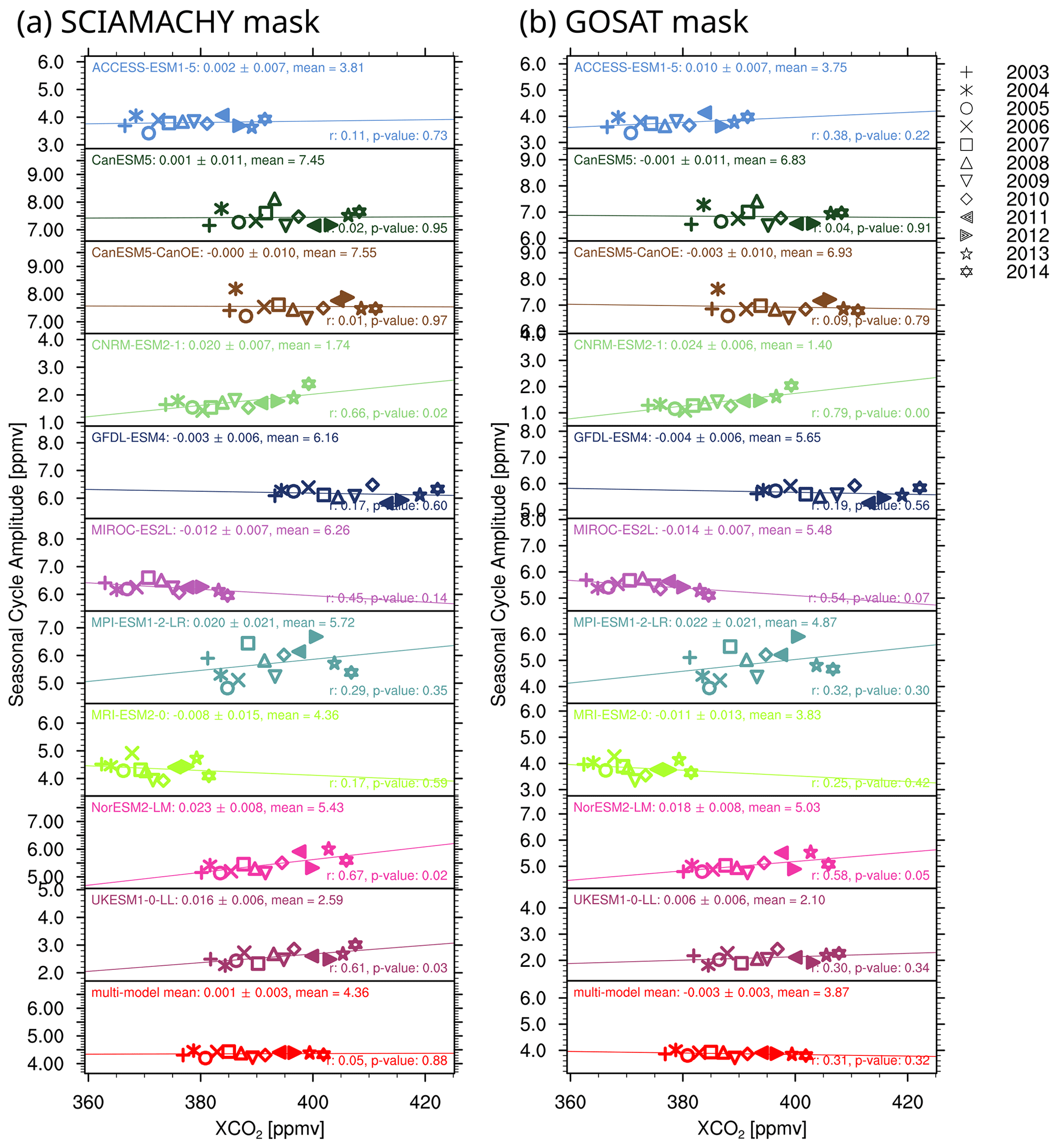
Figure 9Same as Fig. 7 but with CMIP6 models masked using (a) the SCIAMACHY mask and (b) the GOSAT mask, with the masks derived from Fig. 8, masking out points with less than 50 % coverage in those time periods.
Further impacts on CO2 concentrations could come through temporal sampling, such as the fact that the satellite data only include measurements with low cloud cover and are limited to 13:00 LT. While cloud cover can impact photosynthesis, the response can be fundamentally different for various ecosystems (Still et al., 2009); we expect a larger effect from the diurnal cycle in CO2 which is included in the model means but not the satellite data. Due to a lack of CO2 data from models with a higher temporal resolution, this effect cannot be estimated in this study.
In this paper, we have evaluated the performance of CMIP5 and CMIP6 ESMs with interactive carbon cycle (Tables 2 and 3) against column-integral CO2 (XCO2) data from satellite retrievals. Our analysis has compared ESM simulations to the 2003–2014 Obs4MIPs XCO2 satellite dataset O4Mv3 retrieved from radiance spectra measured by the SCIAMACHY/Envisat (2003–2012) and TANSO-FTS/GOSAT (2009–2014) satellite instruments. The O4Mv3 data product has a spatial resolution of and monthly time resolution. For CMIP5, the historical simulations covering the period 2003–2005 were combined with simulations from the RCP8.5 scenario (2006–2014), and for CMIP6 the historical simulations were used (2003–2014). The evaluation of the CMIP models with the satellite data focused on the time series, the GR and the SCA XCO2. All SCAs computed with a masked time series are considered to be “effective” SCAs due to the possibility of masking out peaks and troughs.
The XCO2 time series comparison shows that most models overestimate the carbon content of the atmosphere relative to the satellite observations in both model ensembles, with a lower overestimation for the CMIP6 models of 2 ppmv for the multi-model mean and a wide range of individual model differences of −15 to +20 ppmv. The CMIP5 models overestimate by 5 to 25 ppmv with the exception of the MRI-ESM1 model, which underestimates by 20 ppmv. The CMIP5 multi-model mean overestimates by 10 ppmv compared to the observations, which has also previously been found for surface comparisons (Friedlingstein et al., 2014; Hoffman et al., 2014). Overall, CMIP6 models follow the same trends as their CMIP5 counterparts but with reduced systematic biases.
The XCO2 annual mean growth rate is typically slightly overestimated compared to the observational value of 1.9 ± 0.4 ppmv yr−1. CMIP6 models range from 1.7 ± 0.4 (MRI-ESM2.0) to 2.6 ± 0.7 ppmv yr−1 (GFDL-ESM4) with a multi-model mean of 2.3 ± 0.3 ppmv yr−1. CMIP5 models have a slightly higher multi-model mean growth rate of 2.4 ± 0.4 ppmv yr−1 and a larger spread, with the CMIP5 lowest model being MRI-ESM1 at 1.5 ± 0.4 ppmv yr−1 and the highest CMIP5 growth rate shown by CanESM2 at 3.0 ± 0.9 ppmv yr−1.
All models capture the expected increase of the SCA with increasing latitudes, but most models underestimate the SCA to differing degrees in different regions. This result is in line with previous studies (Wenzel et al., 2016; Graven et al., 2013). Models with similar model components show similar behavior, with models including a nitrogen cycle generally showing a lower SCA in CMIP5, but this influence is not clear in CMIP6. Finally, the connection between SCA and XCO2 was investigated in the northern midlatitudes. Most models from both ensembles show a positive trend, i.e., an increase of the SCA with XCO2, consistent with findings for surface CO2 (Wenzel et al., 2016). However, the satellite product shows a strong negative trend in contrast to the models and surface based observations. We have attributed this trend reversal to the sampling characteristics of the satellite products. The average effective SCA is higher for models sampled according to the SCIAMACHY/Envisat as opposed to the TANSO-FTS/GOSAT mean data coverage. As the early time series is based solely on the SCIAMACHY/Envisat data and the last years only use data from TANSO-FTS/GOSAT, this introduces an artificial negative trend which dominates the positive trend shown by the unsampled models. This demonstrates the importance of equal sampling of models and observations in model evaluation studies.
There are several ways to improve on this analysis in the future. With more available future scenario simulations, the analysis can be extended to a longer time series, making use of longer observational time series, such as the one introduced in Reuter et al. (2020). Higher temporal resolution of the models would enable studies on the effect of the diurnal cycle of CO2 on the monthly mean and also allow for the construction of a co-located time series with the level-2 satellite data. This could help highlight some of the causes of model biases by being able to pinpoint time and space where they occur more precisely. Model biases may also result from the CMIP experimental design, such as requiring the climate state to be in equilibrium in 1850 while the real world may not have been (Bronselaer et al., 2017), or the parameterizations of biological and physical processes not allowing the system to change rapidly enough (Hoffman et al., 2014). Along with a longer time series, newer satellites, such as OCO-2 or the planned Sentinel 7 bring higher resolutions and more data, potentially helping to fill the gaps and reduce the impact of the sampling we discussed in Sect. 5.3.2.
Overall, the CMIP6 ensemble shows improved agreement with the satellite data in all considered quantities (mean XCO2, growth rate, SCA and trend in SCA), with the biggest improvement shown in the mean XCO2 content of the atmosphere. The paper demonstrates the great potential of satellite data for climate model evaluation as this allows us to go beyond regional means or single point observations from in situ data and also enables the investigation of regional effects on SCA, such as the increase in SCA at higher latitudes.
Here, we document the general procedure used to compute model XCO2 for comparison with the satellite-based Obs4MIPs product following the description in Buchwitz and Reuter (2016).
Here, represents the modeled CO2 dry-air mole fraction on model layers (i.e., layer centers or full levels) and nd the number of dry-air particles (air molecules excluding water vapor) within these levels. The summations are performed over all model layers. The number of dry-air particles can be computed as follows:
Na is the Avogadro constant () and md the molar mass of dry air (). Δp is the pressure difference (in hPa) computed from the model's pressure levels (i.e., layer boundaries or half levels) surrounding the model layers, q is the modeled specific humidity (in kg/kg), and g is the gravitational acceleration approximated by
This includes the model's geopotential ϕ (in m2 s−2) on layers, the free air correction constant and the gravitational acceleration g0 on the geoid approximated by the international gravity formula depending only on the latitude φ:
The analysis from Sect. 5.3.2 on the influence of the satellite data mean coverage on the trend of the SCA was also performed for CMIP5. Figures B1 and B2 are the CMIP5 equivalent of Figs. 8 and 10. The CMIP5 models support the analysis of the CMIP6 models and show that the different satellite data coverage results in a different mean effective SCA, with a higher mean effective SCA for SCIAMACHY (2003–2012) than GOSAT (2009–2014) mean data coverage, which overshadows the positive trend and causes it to flip to a negative one in most models.
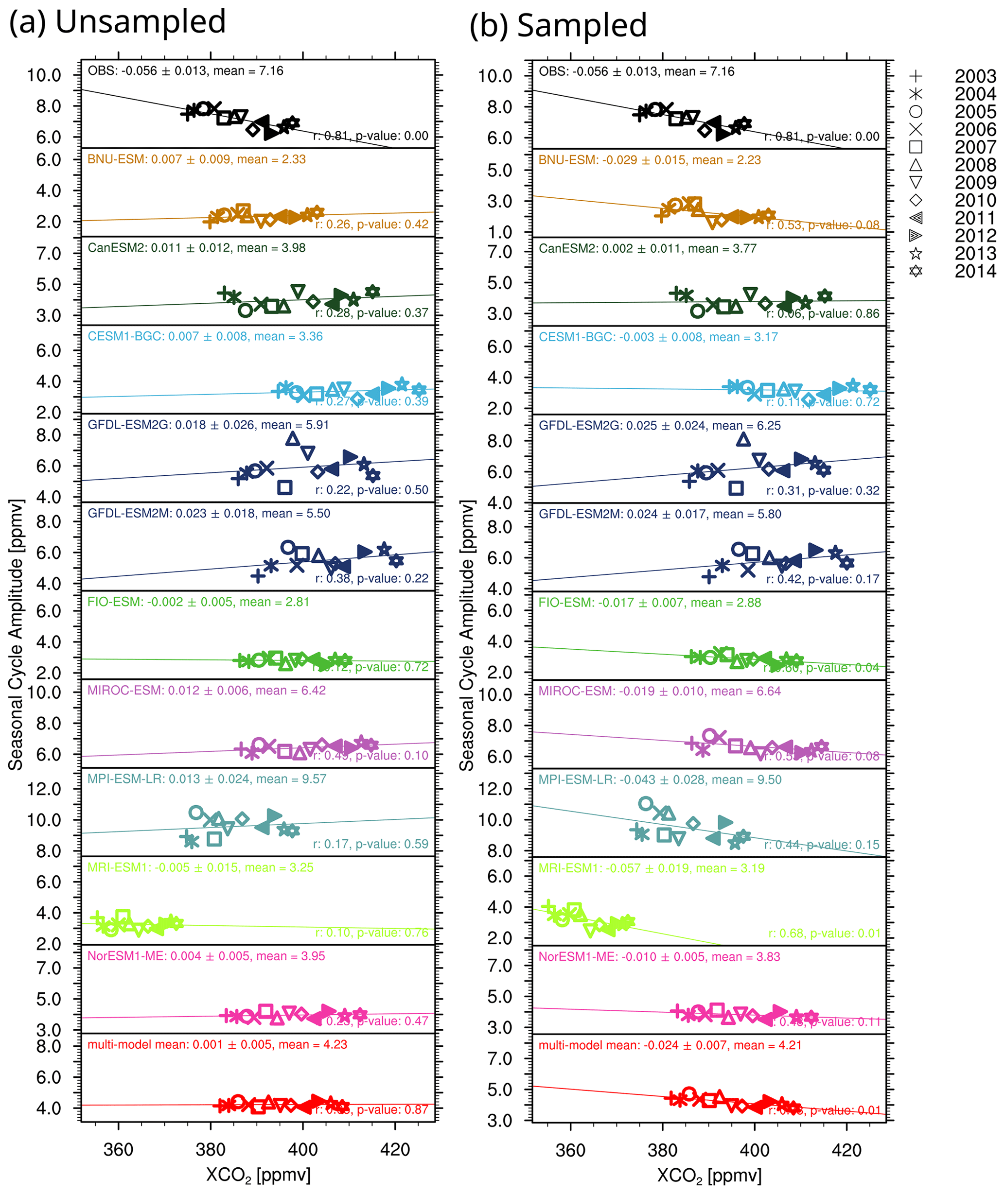
Figure B1Same as Fig. 7 but for CMIP5 models. The left panels (a) show unsampled models, while models sampled according to the satellite data are shown on the right (b). Note that the y-axis range is the same and only differs by a shift.
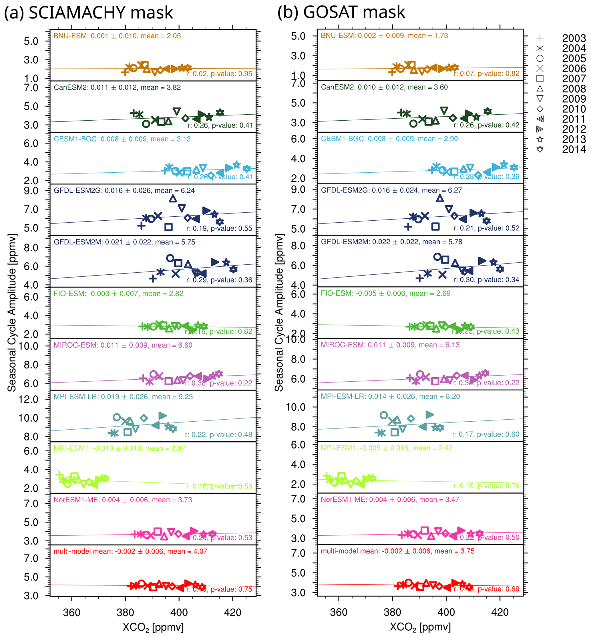
Figure B2Same as Fig. B1 but with CMIP5 models masked using (a) the SCIAMACHY mask and (b) the GOSAT mask, with the masks derived from Fig. 8, masking out points with less than 50 % coverage in those time periods.
Cox et al. (2013) developed an emergent constraint on the sensitivity of tropical land carbon to climate change using the sensitivity of the IAV of CO2 growth rate to the IAV of tropical temperature, which was later adapted by Wenzel et al. (2014) to CMIP5 models. Figure C1 shows the sensitivity of the IAV of XCO2 growth rate to the tropical growing season temperature IAV for CMIP6 (left) and CMIP5 (right) models, both compared with observations. The observational temperature is taken from the GISTEMP v4 dataset (Lenssen et al., 2019) and the models use their own modeled temperature. We find an observational value of −0.23 ± 0.70 ppmv yr−1 K−1 for the 2003–2014 period. However, when using the full span of the satellite data until 2016, the slope increases to 0.75 ± 0.6 ppmv yr−1 K−1 (not shown), as the additional years show both a high growing season temperature and GR IAV, coinciding with a strong El Niño. This shows that the time period 2003–2014 is not sufficiently long to reproduce the emergent constraint, although this may become feasible once CMIP6 emission-driven future simulations are available for a longer time overlap between models and observations. CMIP5 model values for the timeframe 2003–2014 range from 0.53 ± 0.51 (NorESM1-ME) to 3.14 ± 0.63 ppmv yr−1 K−1 (MRI-ESM1), with only CESM1-BGC showing a negative trend of −0.64 ± 0.55 ppmv yr−1 K−1. The multi-model mean has a value of 1.79 ± 0.80 ppmv yr−1 K−1. In CMIP6, the range is significantly decreased with a minimum of 1.14 ± 0.56 ppmv yr−1 K−1 (ACCESS-ESM1.5) to a maximum of 3.37 ± 0.71 ppmv yr−1 K−1 (CanESM5-CanOE) and a multi-model mean of 1.14 ± 0.37 ppmv yr−1 K−1.
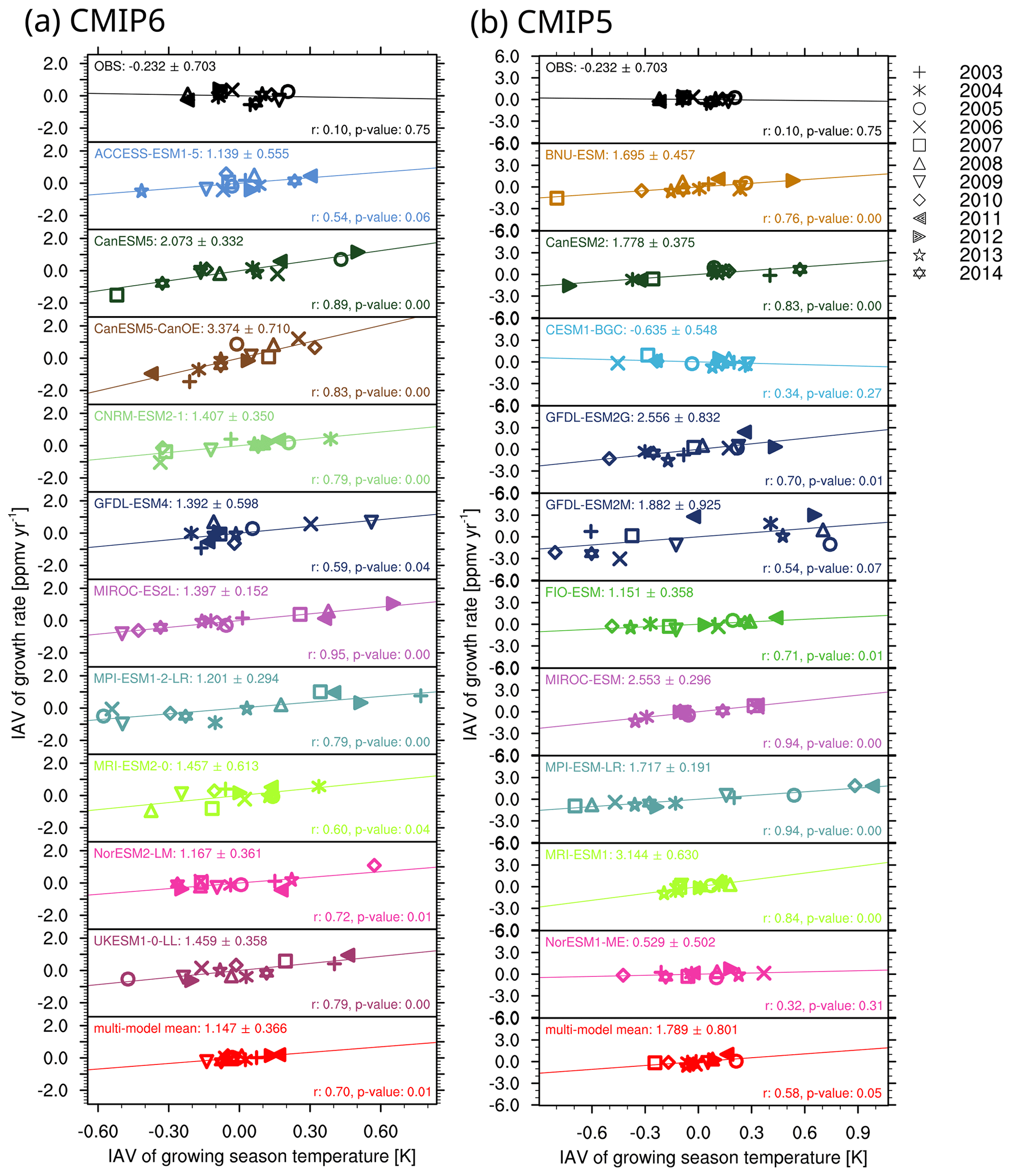
Figure C1Sensitivity of the interannual variability of the XCO2 growth rate in the tropics (30∘ S–30∘ N) to the interannual variability of tropical growing season temperature for CMIP6 models (a) and CMIP5 models (b). The observational temperature taken from the GISTEMP temperature anomaly map, while the models use their own simulated temperature. A linear regression is performed on the data for each dataset. Model colors are the same as in Fig. 3, and symbols denote the years. In the top left of each panel, the regression coefficient and its uncertainty is shown, while the bottom right states the Pearson correlation coefficient and p value.
The O4Mv3 XCO2 data product is available via the Copernicus Climate Change Service (C3S, https://climate.copernicus.eu/, Reuter, 2018) Climate Data Store (CDS) (https://cds.climate.copernicus.eu/, Reuter, 2018), accessed August 2018. The surface flasks measurements were obtained online (ftp://aftp.cmdl.noaa.gov/data/trace_gases/co2/flask/surface/, Dlugokencky et al., 2018), last access: August 2018. Surface temperature anomalies were obtained from the GISTEMP Team, 2020: GISS Surface Temperature Analysis (GISTEMP) version 4, NASA Goddard Institute for Space Studies dataset at https://data.giss.nasa.gov/gistemp/ (GISTEMP Team, 2020, last access: 13 February 2020). The MODIS IGBP land cover type classification was obtained from http://glcf.umd.edu/data/lc/, Friedl et al., 2010b, last access: 31 January 2018). CMIP5 data are freely and publicly available from the Earth System Grid Federation (ESGF, Williams et al. 2009), with CMIP6 data DOIs given in Table 3. ESMValTool v2.0 (Eyring et al., 2020; Lauer et al., 2020; Righi et al., 2020) is released under the Apache License, VERSION 2.0. The latest release of ESMValTool v2 is publicly available on Zenodo at https://doi.org/10.5281/zenodo.3401363 (Andela et al., 2020a). The source code of the ESMValCore package, which is installed as a dependency of the ESMValTool v2, is also publicly available on Zenodo at https://doi.org/10.5281/zenodo.3387139 (Andela et al., 2020b). ESMValTool and ESMValCore are developed on the GitHub repositories available at https://github.com/ESMValGroup, last access: 30 November 2020. The corresponding recipe that can be used to reproduce the figures of this paper will be included in ESMValTool v2 at the time of publication of the paper.
BG led the writing and analysis of the paper. MB and MR provided the satellite dataset. VE, PC and PF contributed to the evaluation of the CMIP simulations. All authors contributed to the writing of the manuscript.
The authors declare that they have no conflict of interest.
This work has been supported by ESA Climate Change Initiative (CCI) Climate Modelling User Group (CMUG) project, the Horizon 2020 project Climate-Carbon Interactions in the Current Century (4C) funded by the EU (grant agreement no. 821003) and the EVal4CMIP project funded by the Helmholtz Society. The generation of the satellite XCO2 data product has received funding from ESA (GHG-CCI) and the EU (Copernicus Climate Change Service – C3S, led by ECMWF). We acknowledge the World Climate Research Programme (WCRP), which, through its Working Group on Coupled Modelling, coordinated and promoted CMIP6. We thank the climate modeling groups (listed in Tables 2 and 3 of this paper) for producing and making available their model output, the Earth System Grid Federation (ESGF) for archiving the data and providing access and the multiple funding agencies who support CMIP and ESGF.
We also thank both anonymous reviewers for their helpful comments on this paper and the handling editor, Trevor Keenan, for taking on this paper.
This research has been supported by Horizon 2020 (grant no. 4C(821003)), the European Space Agency (ESA Climate Change Initiative Climate Model User Group, ESA CCICMUG) and the Helmholtz Association (Advanced Earth SystemModel Evaluation for CMIP, EVal4CMIP).
The article processing charges for this open-access publication were covered by the University of Bremen.
This paper was edited by Trevor Keenan and reviewed by two anonymous referees.
Adachi, Y., Yukimoto, S., Deushi, M., Obata, A., Nakano, H., Tanaka, T. Y., Hosaka, M., Sakami, T., Yoshimura, H., Hirabara, M., Shindo, E., Tsujino, H., Mizuta, R., Yabu, S., Koshiro, T., Ose, T., and Kitoh, A.: Basic performance of a new earth system model of the Meteorological Research Institute (MRI-ESM1), Pap. Meteorol. Geophys., 64, 1–19, https://doi.org/10.2467/mripapers.64.1, 2013.
Anav, A., Friedlingstein, P., Kidston, M., Bopp, L., Ciais, P., Cox, P., Jones, C., Jung, M., Myneni, R., and Zhu, Z.: Evaluating the Land and Ocean Components of the Global Carbon Cycle in the CMIP5 Earth System Models, J. Climate, 26, 6801–6843, https://doi.org/10.1175/Jcli-D-12-00417.1, 2013.
Andela, B., Broetz, B., de Mora, L., Drost, N., Eyring, V., Koldunov,N., Lauer, A., Mueller, B., Predoi, V., Righi, M., Schlund, M.,Vegas-Regidor, J., Zimmermann, K., Adeniyi, K., Arnone, E.,Bellprat, O., Berg, P., Bock, L., Caron, L.-P., Carvalhais, N., Cionni, I., Cortesi, N., Corti, S., Crezee, B., Davin, E. L., Davini,P., Deser, C., Diblen, F., Docquier, D., Dreyer, L., Ehbrecht,C., Earnshaw, P., Gier, B., Gonzalez-Reviriego, N., Goodman,P., Hagemann, S., von Hardenberg, J., Hassler, B., Hunter, A., Kadow, C., Kindermann, S., Koirala, S., Lledó, L., Lejeune, Q.,Lembo, V., Little, B., Loosveldt-Tomas, S., Lorenz, R., Lovato,T., Lucarini, V., Massonnet, F., Mohr, C. W., Amarjiit, P., Pérez-Zanón, N., Phillips, A., Russell, J., Sandstad, M., Sellar, A., Sen-ftleben, D., Serva, F., Sillmann, J., Stacke, T., Swaminathan, R., Torralba, V., and Weigel, K.: ESMValTool (Version v2.0.0), Zenodo, https://doi.org/10.5281/zenodo.3401363, 2020a.
Andela, B., Broetz, B., de Mora, L., Drost, N., Eyring, V., Koldunov, N., Lauer, A., Predoi, V., Righi, M., Schlund, M., Vegas-Regidor, J., Zimmermann, K., Bock, L., Diblen, F., Dreyer, L., Earnshaw, P., Hassler, B., Little, B., Loosveldt-Tomas, S., Smeets, S., Camphuijsen, J., Gier, B.K., Weigel, K., Hauser, M., Kalverla, P., Galytska, E., Cos-Espuña, P., Pelupessy, I., Koirala, S., Stacke, T., Alidoost, S., and Jury, M.: ESMValCore, https://doi.org/10.5281/zenodo.3387139, 2020b.
Arora, V. K., Scinocca, J. F., Boer, G. J., Christian, J. R., Denman, K. L., Flato, G. M., Kharin, V. V., Lee, W. G., and Merryfield, W. J.: Carbon emission limits required to satisfy future representative concentration pathways of greenhouse gases, Geophys. Res. Lett., 38, L05805, https://doi.org/10.1029/2010gl046270, 2011.
Arora, V. K., Boer, G. J., Friedlingstein, P., Eby, M., Jones, C. D., Christian, J. R., Bonan, G., Bopp, L., Brovkin, V., Cadule, P., Hajima, T., Ilyina, T., Lindsay, K., Tjiputra, J. F., and Wu, T.: Carbon-Concentration and Carbon-Climate Feedbacks in CMIP5 Earth System Models, J. Climate, 26, 5289–5314, https://doi.org/10.1175/Jcli-D-12-00494.1, 2013.
Arora, V. K., Katavouta, A., Williams, R. G., Jones, C. D., Brovkin, V., Friedlingstein, P., Schwinger, J., Bopp, L., Boucher, O., Cadule, P., Chamberlain, M. A., Christian, J. R., Delire, C., Fisher, R. A., Hajima, T., Ilyina, T., Joetzjer, E., Kawamiya, M., Koven, C. D., Krasting, J. P., Law, R. M., Lawrence, D. M., Lenton, A., Lindsay, K., Pongratz, J., Raddatz, T., Séférian, R., Tachiiri, K., Tjiputra, J. F., Wiltshire, A., Wu, T., and Ziehn, T.: Carbon–concentration and carbon–climate feedbacks in CMIP6 models and their comparison to CMIP5 models, Biogeosciences, 17, 4173–4222, https://doi.org/10.5194/bg-17-4173-2020, 2020.
Bao, Y., Qiao, F., and Song, Z.: The historical global carbon cycle simulation of FIO-ESM, Geo-phys. Res. Abstr., EGU2012-6834, EGU General Assembly 2012, Vienna, Austria, 2012.
Barnes, E. A., Parazoo, N., Orbe, C., and Denning, A. S.: Isentropic transport and the seasonal cycle amplitude of CO2, J. Geophys. Res.-Atmos., 121, 8106–8124, https://doi.org/10.1002/2016jd025109, 2016.
Bastos, A., Ciais, P., Chevallier, F., Rödenbeck, C., Ballantyne, A. P., Maignan, F., Yin, Y., Fernández-Martínez, M., Friedlingstein, P., Peñuelas, J., Piao, S. L., Sitch, S., Smith, W. K., Wang, X., Zhu, Z., Haverd, V., Kato, E., Jain, A. K., Lienert, S., Lombardozzi, D., Nabel, J. E. M. S., Peylin, P., Poulter, B., and Zhu, D.: Contrasting effects of CO2 fertilization, land-use change and warming on seasonal amplitude of Northern Hemisphere CO2 exchange, Atmos. Chem. Phys., 19, 12361–12375, https://doi.org/10.5194/acp-19-12361-2019, 2019.
Basu, S., Guerlet, S., Butz, A., Houweling, S., Hasekamp, O., Aben, I., Krummel, P., Steele, P., Langenfelds, R., Torn, M., Biraud, S., Stephens, B., Andrews, A., and Worthy, D.: Global CO2 fluxes estimated from GOSAT retrievals of total column CO2, Atmos. Chem. Phys., 13, 8695–8717, https://doi.org/10.5194/acp-13-8695-2013, 2013.
Bovensmann, H., Burrows, J. P., Buchwitz, M., Frerick, J., Noel, S., Rozanov, V. V., Chance, K. V., and Goede, A. P. H.: SCIAMACHY: Mission objectives and measurement modes, J. Atmos. Sci., 56, 127–150, https://doi.org/10.1175/1520-0469(1999)056<0127:Smoamm>2.0.Co;2, 1999.
Bronselaer, B., Winton, M., Russell, J., Sabine, C. L., and Khatiwala, S.: Agreement of CMIP5 Simulated and Observed Ocean Anthropogenic CO2 Uptake, Geophys. Res. Lett., 44, 298–305, https://doi.org/10.1002/2017gl074435, 2017.
Buchwitz, M. and Reuter, M.: Merged SCIAMACHY/ENVISAT and TANSO-FTS/GOSAT atmospheric column-average dry-air mole fraction of CO2 (XCO2 ) (XCO2_CRDP3_001) – Technical Document, 2016, available at: http://134.102.186.42/?q=webfm_send/330, last access: 30 November 2020.
Buchwitz, M., Reuter, M., Schneising-Weigel, O., Aben, I., Detmers, R. G., Hasekamp, O. P., Boesch, H., Anand, J., Crevoisier, C., and Armante, R.: Product User Guide and Specification (PUGS) – Main document, Technical Report Copernicus Climate Change Service (C3S), Reading, UK, 91 pp., 2017a.
Buchwitz, M., Reuter, M., Schneising-Weigel, O., Aben, I., Detmers, R. G., Hasekamp, O. P., Boesch, H., Anand, J., Crevoisier, C., and Armante, R.: Product Quality Assessment Report (PQAR) – Main document, Technical Report Copernicus Climate Change Service (C3S), Reading, UK, 103 pp., 2017b.
Buchwitz, M., Reuter, M., Schneising, O., Noël, S., Gier, B., Bovensmann, H., Burrows, J. P., Boesch, H., Anand, J., Parker, R. J., Somkuti, P., Detmers, R. G., Hasekamp, O. P., Aben, I., Butz, A., Kuze, A., Suto, H., Yoshida, Y., Crisp, D., and O'Dell, C.: Computation and analysis of atmospheric carbon dioxide annual mean growth rates from satellite observations during 2003–2016, Atmos. Chem. Phys., 18, 17355–17370, https://doi.org/10.5194/acp-18-17355-2018, 2018.
Burrows, J. P., Holzle, E., Goede, A. P. H., Visser, H., and Fricke, W.: Sciamachy – Scanning Imaging Absorption Spectrometer for Atmospheric Chartography, Acta Astronaut., 35, 445–451, https://doi.org/10.1016/0094-5765(94)00278-T, 1995.
Calle, L., Poulter, B., and Patra, P. K.: A segmentation algorithm for characterizing rise and fall segments in seasonal cycles: an application to XCO2 to estimate benchmarks and assess model bias, Atmos. Meas. Tech., 12, 2611–2629, https://doi.org/10.5194/amt-12-2611-2019, 2019.
Chevallier, F., Palmer, P. I., Feng, L., Boesch, H., O'Dell, C. W., and Bousquet, P.: Toward robust and consistent regional CO2 flux estimates from in situ and spaceborne measurements of atmospheric CO2, Geophys. Res. Lett., 41, 1065–1070, https://doi.org/10.1002/2013gl058772, 2014.
Ciais, P., Sabine, C., Bala, G., Bopp, L., Brovkin, V., Canadell, J., Chhabra, A., DeFries, R., Galloway, J., Heimann, M., Jones, C., Le Quéré, C., Myneni, R. B., Piao, S., and Thornton, P.: Carbon and Other Biogeochemical Cycles, in: Climate Change 2013: The Physical Science Basis. Contribution of Working Group I to the Fifth Assessment Report of the Intergovernmental Panel on Climate Change, edited by: Stocker, T. F., Qin, D., Plattner, G.-K., Tignor, M., Allen, S. K., Boschung, J., Nauels, A., Xia, Y., Bex, V., and Midgley, P. M., Cambridge University Press, Cambridge, United Kingdom and New York, NY, USA, 465–570, https://doi.org/10.1017/CBO9781107415324.015, 2013.
Cox, P. M., Pearson, D., Booth, B. B., Friedlingstein, P., Huntingford, C., Jones, C. D., and Luke, C. M.: Sensitivity of tropical carbon to climate change constrained by carbon dioxide variability, Nature, 494, 341–344, https://doi.org/10.1038/nature11882, 2013.
Dlugokencky, E. J., Lang, P. M., Mund, J. W., Crotwell, A. M., Crotwell, M. J., and Thoning, K. W.: Atmospheric Carbon Dioxide Dry Air Mole Fractions from the NOAA ESRL Carbon Cycle Cooperative Global Air Sampling Network, available at: ftp://aftp.cmdl.noaa.gov/data/trace_gases/co2/flask/surface/ (last access: 31 July 2018), 2018.
Dlugokencky, E. J., Mund, J. W., Crotwell, A. M., Crotwell, M. J., and Thoning, K. W.: Atmospheric Carbon Dioxide Dry Air Mole Fractions from the NOAA GML Carbon Cycle Cooperative Global Air Sampling Network, 1968–2019, 2020.
Dunne, J. P., John, J. G., Adcroft, A. J., Griffies, S. M., Hallberg, R. W., Shevliakova, E., Stouffer, R. J., Cooke, W., Dunne, K. A., Harrison, M. J., Krasting, J. P., Malyshev, S. L., Milly, P. C. D., Phillipps, P. J., Sentman, L. T., Samuels, B. L., Spelman, M. J., Winton, M., Wittenberg, A. T., and Zadeh, N.: GFDL's ESM2 Global Coupled Climate-Carbon Earth System Models. Part I: Physical Formulation and Baseline Simulation Characteristics, J. Climate, 25, 6646–6665, https://doi.org/10.1175/Jcli-D-11-00560.1, 2012.
Dunne, J. P., John, J. G., Shevliakova, E., Stouffer, R. J., Krasting, J. P., Malyshev, S. L., Milly, P. C. D., Sentman, L. T., Adcroft, A. J., Cooke, W., Dunne, K. A., Griffies, S. M., Hallberg, R. W., Harrison, M. J., Levy, H., Wittenberg, A. T., Phillips, P. J., and Zadeh, N.: GFDL's ESM2 Global Coupled Climate-Carbon Earth System Models. Part II: Carbon System Formulation and Baseline Simulation Characteristics, J. Climate, 26, 2247–2267, https://doi.org/10.1175/Jcli-D-12-00150.1, 2013.
Dunne, J. P., Horowitz, L. W., Adcroft, A. J., Ginoux, P., Held, I. M., John, J. G., Krasting, J. P., Malyshev, S., Naik, V., Paulot, F., Shevliakova, E., Stock, C. A., Zadeh, N., Balaji, V., Blanton, C., Dunne, K. A., Dupuis, C., Durachta, J., Dussin, R., Gauthier, P. P. G., Griffies, S. M., Guo, H., Hallberg, R. W., Harrison, M., He, J., Hurlin, W., McHugh, C., Menzel, R., Milly, P. C. D., Nikonov, S., Paynter, D. J., Ploshay, J., Radhakrishnan, A., Rand, K., Reichl, B. G., Robinson, T., Schwarzkopf, D. M., Sentman, L. T., Underwood, S., Vahlenkamp, H., Winton, M., Wittenberg, A. T., Wyman, B., Zeng, Y., and Zhao, M.: The GFDL Earth System Model version 4.1 (GFDL-ESM 4.1): Overall coupled model description and simulation characteristics, J. Adv. Model. Earth. Sy., 12, e2019MS002015, https://doi.org/10.1029/2019ms002015, 2020.
Eyring, V., Bony, S., Meehl, G. A., Senior, C. A., Stevens, B., Stouffer, R. J., and Taylor, K. E.: Overview of the Coupled Model Intercomparison Project Phase 6 (CMIP6) experimental design and organization, Geosci. Model Dev., 9, 1937–1958, https://doi.org/10.5194/gmd-9-1937-2016, 2016a.
Eyring, V., Righi, M., Lauer, A., Evaldsson, M., Wenzel, S., Jones, C., Anav, A., Andrews, O., Cionni, I., Davin, E. L., Deser, C., Ehbrecht, C., Friedlingstein, P., Gleckler, P., Gottschaldt, K.-D., Hagemann, S., Juckes, M., Kindermann, S., Krasting, J., Kunert, D., Levine, R., Loew, A., Mäkelä, J., Martin, G., Mason, E., Phillips, A. S., Read, S., Rio, C., Roehrig, R., Senftleben, D., Sterl, A., van Ulft, L. H., Walton, J., Wang, S., and Williams, K. D.: ESMValTool (v1.0) – a community diagnostic and performance metrics tool for routine evaluation of Earth system models in CMIP, Geosci. Model Dev., 9, 1747–1802, https://doi.org/10.5194/gmd-9-1747-2016, 2016b.
Eyring, V., Cox, P. M., Flato, G. M., Gleckler, P. J., Abramowitz, G., Caldwell, P., Collins, W. D., Gier, B. K., Hall, A. D., Hoffman, F. M., Hurtt, G. C., Jahn, A., Jones, C. D., Klein, S. A., Krasting, J. P., Kwiatkowski, L., Lorenz, R., Maloney, E., Meehl, G. A., Pendergrass, A. G., Pincus, R., Ruane, A. C., Russell, J. L., Sanderson, B. M., Santer, B. D., Sherwood, S. C., Simpson, I. R., Stouffer, R. J., and Williamson, M. S.: Taking climate model evaluation to the next level, Nat. Clim. Change, 9, 102–110, https://doi.org/10.1038/s41558-018-0355-y, 2019.
Eyring, V., Bock, L., Lauer, A., Righi, M., Schlund, M., Andela, B., Arnone, E., Bellprat, O., Brötz, B., Caron, L.-P., Carvalhais, N., Cionni, I., Cortesi, N., Crezee, B., Davin, E. L., Davini, P., Debeire, K., de Mora, L., Deser, C., Docquier, D., Earnshaw, P., Ehbrecht, C., Gier, B. K., Gonzalez-Reviriego, N., Goodman, P., Hagemann, S., Hardiman, S., Hassler, B., Hunter, A., Kadow, C., Kindermann, S., Koirala, S., Koldunov, N., Lejeune, Q., Lembo, V., Lovato, T., Lucarini, V., Massonnet, F., Müller, B., Pandde, A., Pérez-Zanón, N., Phillips, A., Predoi, V., Russell, J., Sellar, A., Serva, F., Stacke, T., Swaminathan, R., Torralba, V., Vegas-Regidor, J., von Hardenberg, J., Weigel, K., and Zimmermann, K.: Earth System Model Evaluation Tool (ESMValTool) v2.0 – an extended set of large-scale diagnostics for quasi-operational and comprehensive evaluation of Earth system models in CMIP, Geosci. Model Dev., 13, 3383–3438, https://doi.org/10.5194/gmd-13-3383-2020, 2020.
Fernández-Martínez, M., Sardans, J., Chevallier, F., Ciais, P., Obersteiner, M., Vicca, S., Canadell, J. G., Bastos, A., Friedlingstein, P., Sitch, S., Piao, S. L., Janssens, I. A., and Peñuelas, J.: Global trends in carbon sinks and their relationships with CO2 and temperature, Nat. Clim, Change, 9, 73—9, https://doi.org/10.1038/s41558-018-0367-7, 2019.
Ferraro, R., Waliser, D. E., Gleckler, P., Taylor, K. E., and Eyring, V.: Evolving Obs4MIPs to Support Phase 6 of the Coupled Model Intercomparison Project (CMIP6), B. Am. Meteorol. Soc., 96, 131–133, https://doi.org/10.1175/bams-d-14-00216.1, 2015.
Friedl, M. A., Sulla-Menashe, D., Tan, B., Schneider, A., Ramankutty, N., Sibley, A., and Huang, X. M.: MODIS Collection 5 global land cover: Algorithm refinements and characterization of new datasets, Remote Sens. Environ., 114, 168–182, https://doi.org/10.1016/j.rse.2009.08.016, 2010a.
Friedl, M. A., Strahler, A. H., Hodges, J., Hall, F. G., Collatz, G. J., Meeson, B. W., Los, S. O., Brown De Colstoun, E., and Landis, D. R.: ISLSCP II MODIS (Collection 4) IGBP Land Cover, 2000–2001, ORNL DAAC, Oak Ridge, Tennessee, USA, https://doi.org/doi.org/10.3334/ORNLDAAC/968 (last access: 3 January 2018), 2010b.
Friedlingstein, P., Cox, P., Betts, R., Bopp, L., von Bloh, W., Brovkin, V., Cadule, P., Doney, S., Eby, M., Fung, I., Bala, G., John, J., Jones, C., Joos, F., Kato, T., Kawamiya, M., Knorr, W., Lindsay, K., Matthews, H. D., Raddatz, T., Rayner, P., Reick, C., Roeckner, E., Schnitzler, K. G., Schnur, R., Strassmann, K., Weaver, A. J., Yoshikawa, C., and Zeng, N.: Climate-Carbon Cycle Feedback Analysis: Results from the C4MIP Model Intercomparison, J. Climate, 19, 3337–3353, https://doi.org/10.1175/jcli3800.1, 2006.
Friedlingstein, P., Meinshausen, M., Arora, V. K., Jones, C. D., Anav, A., Liddicoat, S. K., and Knutti, R.: Uncertainties in CMIP5 Climate Projections due to Carbon Cycle Feedbacks, J. Climate, 27, 511–526, https://doi.org/10.1175/Jcli-D-12-00579.1, 2014.
Friedlingstein, P., Jones, M. W., O'Sullivan, M., Andrew, R. M., Hauck, J., Peters, G. P., Peters, W., Pongratz, J., Sitch, S., Le Quéré, C., Bakker, D. C. E., Canadell, J. G., Ciais, P., Jackson, R. B., Anthoni, P., Barbero, L., Bastos, A., Bastrikov, V., Becker, M., Bopp, L., Buitenhuis, E., Chandra, N., Chevallier, F., Chini, L. P., Currie, K. I., Feely, R. A., Gehlen, M., Gilfillan, D., Gkritzalis, T., Goll, D. S., Gruber, N., Gutekunst, S., Harris, I., Haverd, V., Houghton, R. A., Hurtt, G., Ilyina, T., Jain, A. K., Joetzjer, E., Kaplan, J. O., Kato, E., Klein Goldewijk, K., Korsbakken, J. I., Landschützer, P., Lauvset, S. K., Lefèvre, N., Lenton, A., Lienert, S., Lombardozzi, D., Marland, G., McGuire, P. C., Melton, J. R., Metzl, N., Munro, D. R., Nabel, J. E. M. S., Nakaoka, S.-I., Neill, C., Omar, A. M., Ono, T., Peregon, A., Pierrot, D., Poulter, B., Rehder, G., Resplandy, L., Robertson, E., Rödenbeck, C., Séférian, R., Schwinger, J., Smith, N., Tans, P. P., Tian, H., Tilbrook, B., Tubiello, F. N., van der Werf, G. R., Wiltshire, A. J., and Zaehle, S.: Global Carbon Budget 2019, Earth Syst. Sci. Data, 11, 1783–1838, https://doi.org/10.5194/essd-11-1783-2019, 2019.
Gent, P. R., Danabasoglu, G., Donner, L. J., Holland, M. M., Hunke, E. C., Jayne, S. R., Lawrence, D. M., Neale, R. B., Rasch, P. J., Vertenstein, M., Worley, P. H., Yang, Z. L., and Zhang, M. H.: The Community Climate System Model Version 4, J. Climate, 24, 4973–4991, https://doi.org/10.1175/2011jcli4083.1, 2011.
GISTEMP Team: GISS Surface Temperature Analysis (GISTEMP), version 4, NASA Goddard Institute for Space Studies, available at: https://data.giss.nasa.gov/gistemp/, last access: 13 February 2020.
Giorgetta, M. A., Jungclaus, J., Reick, C. H., Legutke, S., Bader, J., Bottinger, M., Brovkin, V., Crueger, T., Esch, M., Fieg, K., Glushak, K., Gayler, V., Haak, H., Hollweg, H. D., Ilyina, T., Kinne, S., Kornblueh, L., Matei, D., Mauritsen, T., Mikolajewicz, U., Mueller, W., Notz, D., Pithan, F., Raddatz, T., Rast, S., Redler, R., Roeckner, E., Schmidt, H., Schnur, R., Segschneider, J., Six, K. D., Stockhause, M., Timmreck, C., Wegner, J., Widmann, H., Wieners, K. H., Claussen, M., Marotzke, J., and Stevens, B.: Climate and carbon cycle changes from 1850 to 2100 in MPI-ESM simulations for the Coupled Model Intercomparison Project phase 5, J. Adv. Model. Earth Sy., 5, 572–597, https://doi.org/10.1002/jame.20038, 2013.
Graven, H. D., Keeling, R. F., Piper, S. C., Patra, P. K., Stephens, B. B., Wofsy, S. C., Welp, L. R., Sweeney, C., Tans, P. P., Kelley, J. J., Daube, B. C., Kort, E. A., Santoni, G. W., and Bent, J. D.: Enhanced seasonal exchange of CO2 by northern ecosystems since 1960, Science, 341, 1085–1089, https://doi.org/10.1126/science.1239207, 2013.
Hajima, T., Tachiiri, K., Ito, A., and Kawamiya, M.: Uncertainty of Concentration-Terrestrial Carbon Feedback in Earth System Models, J. Climate, 27, 3425–3445, https://doi.org/10.1175/Jcli-D-13-00177.1, 2014.
Hajima, T., Abe, M., Arakawa, O., Suzuki, T., Komuro, Y., Ogochi, K., Watanabe, M., Yamamoto, A., Tatebe, H., Noguchi, M. A., Ohgaito, R., Ito, A., Yamazaki, D., Ito, A., Takata, K., Watanabe, S., Kawamiya, M., and Tachiiri, K.: MIROC MIROC-ES2L model output prepared for CMIP6 CMIP esm-hist v20200318, Earth System Grid Federation, https://doi.org/10.22033/ESGF/CMIP6.5496, 2020a.
Hajima, T., Watanabe, M., Yamamoto, A., Tatebe, H., Noguchi, M. A., Abe, M., Ohgaito, R., Ito, A., Yamazaki, D., Okajima, H., Ito, A., Takata, K., Ogochi, K., Watanabe, S., and Kawamiya, M.: Development of the MIROC-ES2L Earth system model and the evaluation of biogeochemical processes and feedbacks, Geosci. Model Dev., 13, 2197–2244, https://doi.org/10.5194/gmd-13-2197-2020, 2020b.
Hansen, J., Ruedy, R., Sato, M., and Lo, K.: Global Surface Temperature Change, Rev. Geophys., 48, 4004, https://doi.org/10.1029/2010rg000345, 2010.
Hayman, G. D., O'Connor, F. M., Dalvi, M., Clark, D. B., Gedney, N., Huntingford, C., Prigent, C., Buchwitz, M., Schneising, O., Burrows, J. P., Wilson, C., Richards, N., and Chipperfield, M.: Comparison of the HadGEM2 climate-chemistry model against in situ and SCIAMACHY atmospheric methane data, Atmos. Chem. Phys., 14, 13257–13280, https://doi.org/10.5194/acp-14-13257-2014, 2014.
Hoffman, F. M., Randerson, J. T., Arora, V. K., Bao, Q., Cadule, P., Ji, D., Jones, C. D., Kawamiya, M., Khatiwala, S., Lindsay, K., Obata, A., Shevliakova, E., Six, K. D., Tjiputra, J. F., Volodin, E. M., and Wu, T.: Causes and implications of persistent atmospheric carbon dioxide biases in Earth System Models, J. Geophys. Res.-Biogeo., 119, 141–162, https://doi.org/10.1002/2013jg002381, 2014.
Houweling, S., Baker, D., Basu, S., Boesch, H., Butz, A., Chevallier, F., Deng, F., Dlugokencky, E. J., Feng, L., Ganshin, A., Hasekamp, O., Jones, D., Maksyutov, S., Marshall, J., Oda, T., O'Dell, C. W., Oshchepkov, S., Palmer, P. I., Peylin, P., Poussi, Z., Reum, F., Takagi, H., Yoshida, Y., and Zhuravlev, R.: An intercomparison of inverse models for estimating sources and sinks of CO2 using GOSAT measurements, J. Geophys. Res.-Atmos., 120, 5253–5266, https://doi.org/10.1002/2014jd022962, 2015.
IPCC: Climate Change 2013: The Physical Science Basis. Contribution of Working Group I to the Fifth Assessment Report of the Intergovernmental Panel on Climate Change, Cambridge University Press, Cambridge, UK, https://doi.org/10.1017/CBO9781107415324, 2013.
Ji, D., Wang, L., Feng, J., Wu, Q., Cheng, H., Zhang, Q., Yang, J., Dong, W., Dai, Y., Gong, D., Zhang, R.-H., Wang, X., Liu, J., Moore, J. C., Chen, D., and Zhou, M.: Description and basic evaluation of Beijing Normal University Earth System Model (BNU-ESM) version 1, Geosci. Model Dev., 7, 2039–2064, https://doi.org/10.5194/gmd-7-2039-2014, 2014.
Kaminski, T., Knorr, W., Schurmann, G., Scholze, M., Rayner, P. J., Zaehle, S., Blessing, S., Dorigo, W., Gayler, V., Giering, R., Gobron, N., Grant, J. P., Heimann, M., Hooker-Stroud, A., Houweling, S., Kato, T., Kattge, J., Kelley, D., Kemp, S., Koffi, E. N., Kostler, C., Mathieu, P. P., Pinty, B., Reick, C. H., Rodenbeck, C., Schnur, R., Scipal, K., Sebald, C., Stacke, T., van Scheltinga, A. T., Vossbeck, M., Widmann, H., and Ziehn, T.: The BETHY/JSBACH Carbon Cycle Data Assimilation System: experiences and challenges, J. Geophys. Res.-Biogeo., 118, 1414–1426, https://doi.org/10.1002/jgrg.20118, 2013.
Keeling, C. D., Bacastow, R. B., Bainbridge, A. E., Ekdahl, C. A., Guenther, P. R., Waterman, L. S., and Chin, J. F. S.: Atmospheric Carbon-Dioxide Variations at Mauna-Loa Observatory, Hawaii, Tellus, 28, 538–551, https://doi.org/10.1111/j.2153-3490.1976.tb00701.x, 1976.
Keeling, C. D., Bacastow, R. B., Carter, A. F., Piper, S. C., Whorf, T. P., Heimann, M., Mook, W. G., and Roeloffzen, H.: A three-dimensional model of atmospheric CO2 transport based on observed winds: 1. Analysis of observational data, in: Aspects of Climate Variability in the Pacific and the Western Americas, edited by: Peterson, D. H., American Geophysical Union, Washington, DC, 165–236, 1989.
Keeling, C. D., Whorf, T. P., Wahlen, M., and Vanderplicht, J.: Interannual Extremes in the Rate of Rise of Atmospheric Carbon-Dioxide since 1980, Nature, 375, 666–670, https://doi.org/10.1038/375666a0, 1995.
Keeling, C. D., Chin, J. F. S., and Whorf, T. P.: Increased activity of northern vegetation inferred from atmospheric CO2 measurements, Nature, 382, 146–149, https://doi.org/10.1038/382146a0, 1996.
Krasting, J. P., John, J. G., Blanton, C., McHugh, C., Nikonov, S., Radhakrishnan, A., Rand, K., Zadeh, N. T., Balaji, V., Durachta, J., Dupuis, C., Menzel, R., Robinson, T., Underwood, S., Vahlenkamp, H., Dunne, K. A., Gauthier, P. P. G., Ginoux, P., Griffies, S. M., Hallberg, R., Harrison, M., Hurlin, W., Malyshev, S., Naik, V., Paulot, F., Paynter, D. J., Ploshay, J., Schwarzkopf, D. M., Seman, C. J., Silvers, L., Wyman, B., Zeng, Y., Adcroft, A., Dunne, J. P., Dussin, R., Guo, H., He, J., Held, I. M., Horowitz, L. W., Lin, P., Milly, P. C. D., Shevliakova, E., Stock, C., Winton, M., Xie, Y., and Zhao, M.: NOAA-GFDL GFDL-ESM4 model output prepared for CMIP6 CMIP esm-hist v20190829, Earth System Grid Federation, https://doi.org/10.22033/ESGF/CMIP6.8522, 2018.
Kuze, A., Suto, H., Nakajima, M., and Hamazaki, T.: Thermal and near infrared sensor for carbon observation Fourier-transform spectrometer on the Greenhouse Gases Observing Satellite for greenhouse gases monitoring, Appl. Opt., 48, 6716–6733, https://doi.org/10.1364/AO.48.006716, 2009.
Lauer, A., Eyring, V., Bellprat, O., Bock, L., Gier, B. K., Hunter, A., Lorenz, R., Pérez-Zanón, N., Righi, M., Schlund, M., Senftleben, D., Weigel, K., and Zechlau, S.: Earth System Model Evaluation Tool (ESMValTool) v2.0 – diagnostics for emergent constraints and future projections from Earth system models in CMIP, Geosci. Model Dev., 13, 4205–4228, https://doi.org/10.5194/gmd-13-4205-2020, 2020.
Law, R. M., Ziehn, T., Matear, R. J., Lenton, A., Chamberlain, M. A., Stevens, L. E., Wang, Y.-P., Srbinovsky, J., Bi, D., Yan, H., and Vohralik, P. F.: The carbon cycle in the Australian Community Climate and Earth System Simulator (ACCESS-ESM1) – Part 1: Model description and pre-industrial simulation, Geosci. Model Dev., 10, 2567–2590, https://doi.org/10.5194/gmd-10-2567-2017, 2017.
Lenssen, N. J. L., Schmidt, G. A., Hansen, J. E., Menne, M. J., Persin, A., Ruedy, R., and Zyss, D.: Improvements in the GISTEMP Uncertainty Model, J. Geophys. Res.-Atmos., 124, 6307–6326, https://doi.org/10.1029/2018jd029522, 2019.
Lindsay, K., Bonan, G. B., Doney, S. C., Hoffman, F. M., Lawrence, D. M., Long, M. C., Mahowald, N. M., Moore, J. K., Randerson, J. T., and Thornton, P. E.: Preindustrial-Control and Twentieth-Century Carbon Cycle Experiments with the Earth System Model CESM1 (BGC), J. Climate, 27, 8981–9005, https://doi.org/10.1175/Jcli-D-12-00565.1, 2014.
Mauritsen, T., Bader, J., Becker, T., Behrens, J., Bittner, M., Brokopf, R., Brovkin, V., Claussen, M., Crueger, T., Esch, M., Fast, I., Fiedler, S., Fläschner, D., Gayler, V., Giorgetta, M., Goll, D. S., Haak, H., Hagemann, S., Hedemann, C., Hohenegger, C., Ilyina, T., Jahns, T., Jimenéz-de-la-Cuesta, D., Jungclaus, J., Kleinen, T., Kloster, S., Kracher, D., Kinne, S., Kleberg, D., Lasslop, G., Kornblueh, L., Marotzke, J., Matei, D., Meraner, K., Mikolajewicz, U., Modali, K., Möbis, B., Müller, W. A., Nabel, J. E. M. S., Nam, C. C. W., Notz, D., Nyawira, S.-S., Paulsen, H., Peters, K., Pincus, R., Pohlmann, H., Pongratz, J., Popp, M., Raddatz, T. J., Rast, S., Redler, R., Reick, C. H., Rohrschneider, T., Schemann, V., Schmidt, H., Schnur, R., Schulzweida, U., Six, K. D., Stein, L., Stemmler, I., Stevens, B., von Storch, J.-S., Tian, F., Voigt, A., Vrese, P., Wieners, K.-H., Wilkenskjeld, S., Winkler, A., and Roeckner, E.: Developments in the MPI-M Earth System Model version 1.2 (MPI-ESM1.2) and Its Response to Increasing CO2, J. Adv. Model. Earth. Sy., 11, 998–1038, https://doi.org/10.1029/2018ms001400, 2019.
Myneni, R. B., Keeling, C. D., Tucker, C. J., Asrar, G., and Nemani, R. R.: Increased plant growth in the northern high latitudes from 1981 to 1991, Nature, 386, 698–702, https://doi.org/10.1038/386698a0, 1997.
Piao, S., Liu, Z., Wang, Y., Ciais, P., Yao, Y., Peng, S., Chevallier, F., Friedlingstein, P., Janssens, I. A., Peñuelas, J., Sitch, S., and Wang, T.: On the causes of trends in the seasonal amplitude of atmospheric CO2, Glob. Change Biol., 24, 608–616, https://doi.org/10.1111/gcb.13909, 2018.
Qiao, F. L., Song, Z. Y., Bao, Y., Song, Y. J., Shu, Q., Huang, C. J., and Zhao, W.: Development and evaluation of an Earth System Model with surface gravity waves, J. Geophys. Res.-Ocean., 118, 4514–4524, https://doi.org/10.1002/jgrc.20327, 2013.
Reich, P. B., Hobbie, S. E., Lee, T., Ellsworth, D. S., West, J. B., Tilman, D., Knops, J. M. H., Naeem, S., and Trost, J.: Nitrogen limitation constrains sustainability of ecosystem response to CO2, Nature, 440, 922–925, https://doi.org/10.1038/nature04486, 2006.
Reuter, M., Bösch, H., Bovensmann, H., Bril, A., Buchwitz, M., Butz, A., Burrows, J. P., O'Dell, C. W., Guerlet, S., Hasekamp, O., Heymann, J., Kikuchi, N., Oshchepkov, S., Parker, R., Pfeifer, S., Schneising, O., Yokota, T., and Yoshida, Y.: A joint effort to deliver satellite retrieved atmospheric CO2 concentrations for surface flux inversions: the ensemble median algorithm EMMA, Atmos. Chem. Phys., 13, 1771–1780, https://doi.org/10.5194/acp-13-1771-2013, 2013.
Reuter, M., Buchwitz, M., Hilker, M., Heymann, J., Schneising, O., Pillai, D., Bovensmann, H., Burrows, J. P., Bösch, H., Parker, R., Butz, A., Hasekamp, O., O'Dell, C. W., Yoshida, Y., Gerbig, C., Nehrkorn, T., Deutscher, N. M., Warneke, T., Notholt, J., Hase, F., Kivi, R., Sussmann, R., Machida, T., Matsueda, H., and Sawa, Y.: Satellite-inferred European carbon sink larger than expected, Atmos. Chem. Phys., 14, 13739–13753, https://doi.org/10.5194/acp-14-13739-2014, 2014.
Reuter, M., Buchwitz, M., and Schneising-Weigel, O.: Product User Guide and Specification (PUGS) – ANNEX D for products XCO2_EMMA and XCH4_EMMA, 1–19, available at: https://www.iup.uni-bremen.de/carbon_ghg/docs/C3S/CDR1_2003-2016/PUGS/C3S_D312a_Lot6.3.1.5-v1_PUGS_ANNEX-D_v1.3.pdf (last access: 30 November 2020), 2017.
Reuter, M.: O4Mv3 XCO2 data product version 3, available at: https://cds.climate.copernicus.eu/cdsapp#!/dataset/satellite-carbon-dioxide?tab=form, last access: 1 August 2018.
Reuter, M., Buchwitz, M., Schneising, O., Noël, S., Bovensmann, H., Burrows, J. P., Boesch, H., Di Noia, A., Anand, J., Parker, R. J., Somkuti, P., Wu, L., Hasekamp, O. P., Aben, I., Kuze, A., Suto, H., Shiomi, K., Yoshida, Y., Morino, I., Crisp, D., O'Dell, C. W., Notholt, J., Petri, C., Warneke, T., Velazco, V. A., Deutscher, N. M., Griffith, D. W. T., Kivi, R., Pollard, D. F., Hase, F., Sussmann, R., Té, Y. V., Strong, K., Roche, S., Sha, M. K., De Mazière, M., Feist, D. G., Iraci, L. T., Roehl, C. M., Retscher, C., and Schepers, D.: Ensemble-based satellite-derived carbon dioxide and methane column-averaged dry-air mole fraction data sets (2003–2018) for carbon and climate applications, Atmos. Meas. Tech., 13, 789–819, https://doi.org/10.5194/amt-13-789-2020, 2020.
Righi, M., Andela, B., Eyring, V., Lauer, A., Predoi, V., Schlund, M., Vegas-Regidor, J., Bock, L., Brötz, B., de Mora, L., Diblen, F., Dreyer, L., Drost, N., Earnshaw, P., Hassler, B., Koldunov, N., Little, B., Loosveldt Tomas, S., and Zimmermann, K.: Earth System Model Evaluation Tool (ESMValTool) v2.0 – technical overview, Geosci. Model Dev., 13, 1179–1199, https://doi.org/10.5194/gmd-13-1179-2020, 2020.
Ryu, Y., Berry, J. A., and Baldocchi, D. D.: What is global photosynthesis? History, uncertainties and opportunities, Remote Sens. Environ., 223, 95–114, https://doi.org/10.1016/j.rse.2019.01.016, 2019.
Schneising, O., Reuter, M., Buchwitz, M., Heymann, J., Bovensmann, H., and Burrows, J. P.: Terrestrial carbon sink observed from space: variation of growth rates and seasonal cycle amplitudes in response to interannual surface temperature variability, Atmos. Chem. Phys., 14, 133–141, https://doi.org/10.5194/acp-14-133-2014, 2014.
Seferian, R.: CNRM-CERFACS CNRM-ESM2-1 model output prepared for CMIP6 CMIP esm-hist v20200715, Earth System Grid Federation, https://doi.org/10.22033/ESGF/CMIP6.4003, 2019.
Séférian, R., Nabat, P., Michou, M., Saint-Martin, D., Voldoire, A., Colin, J., Decharme, B., Delire, C., Berthet, S., Chevallier, M., Sénési, S., Franchisteguy, L., Vial, J., Mallet, M., Joetzjer, E., Geoffroy, O., Guérémy, J.-F., Moine, M.-P., Msadek, R., Ribes, A., Rocher, M., Roehrig, R., Salas-y-Mélia, D., Sanchez, E., Terray, L., Valcke, S., Waldman, R., Aumont, O., Bopp, L., Deshayes, J., Éthé, C., and Madec, G.: Evaluation of CNRM Earth System Model, CNRM-ESM2-1: Role of Earth System Processes in Present-Day and Future Climate, J. Adv. Model. Earth Sy., 11, 4182–4227, https://doi.org/10.1029/2019ms001791, 2019.
Seland, Ø., Bentsen, M., Oliviè, D. J. L., Toniazzo, T., Gjermundsen, A., Graff, L. S., Debernard, J. B., Gupta, A. K., He, Y., Kirkevåg, A., Schwinger, J., Tjiputra, J., Aas, K. S., Bethke, I., Fan, Y., Griesfeller, J., Grini, A., Guo, C., Ilicak, M., Karset, I. H. H., Landgren, O. A., Liakka, J., Moseid, K. O., Nummelin, A., Spensberger, C., Tang, H., Zhang, Z., Heinze, C., Iversen, T., and Schulz, M.: NCC NorESM2-LM model output prepared for CMIP6 CMIP esm-hist v20190920, Earth System Grid Federation, https://doi.org/10.22033/ESGF/CMIP6.7924, 2019.
Seland, Ø., Bentsen, M., Seland Graff, L., Olivié, D., Toniazzo, T., Gjermundsen, A., Debernard, J. B., Gupta, A. K., He, Y., Kirkevåg, A., Schwinger, J., Tjiputra, J., Schancke Aas, K., Bethke, I., Fan, Y., Griesfeller, J., Grini, A., Guo, C., Ilicak, M., Hafsahl Karset, I. H., Landgren, O., Liakka, J., Onsum Moseid, K., Nummelin, A., Spensberger, C., Tang, H., Zhang, Z., Heinze, C., Iverson, T., and Schulz, M.: The Norwegian Earth System Model, NorESM2 – Evaluation of theCMIP6 DECK and historical simulations, Geosci. Model Dev. Discuss., https://doi.org/10.5194/gmd-2019-378, in review, 2020.
Sellar, A. A., Jones, C. G., Mulcahy, J. P., Tang, Y., Yool, A., Wiltshire, A., O'Connor, F. M., Stringer, M., Hill, R., Palmieri, J., Woodward, S., de Mora, L., Kuhlbrodt, T., Rumbold, S. T., Kelley, D. I., Ellis, R., Johnson, C. E., Walton, J., Abraham, N. L., Andrews, M. B., Andrews, T., Archibald, A. T., Berthou, S., Burke, E., Blockley, E., Carslaw, K., Dalvi, M., Edwards, J., Folberth, G. A., Gedney, N., Griffiths, P. T., Harper, A. B., Hendry, M. A., Hewitt, A. J., Johnson, B., Jones, A., Jones, C. D., Keeble, J., Liddicoat, S., Morgenstern, O., Parker, R. J., Predoi, V., Robertson, E., Siahaan, A., Smith, R. S., Swaminathan, R., Woodhouse, M. T., Zeng, G., and Zerroukat, M.: UKESM1: Description and Evaluation of the U.K. Earth System Model, J. Adv. Model. Earth. Sy., 11, 4513–4558, https://doi.org/10.1029/2019MS001739, 2019.
Shindell, D. T., Lamarque, J.-F., Schulz, M., Flanner, M., Jiao, C., Chin, M., Young, P. J., Lee, Y. H., Rotstayn, L., Mahowald, N., Milly, G., Faluvegi, G., Balkanski, Y., Collins, W. J., Conley, A. J., Dalsoren, S., Easter, R., Ghan, S., Horowitz, L., Liu, X., Myhre, G., Nagashima, T., Naik, V., Rumbold, S. T., Skeie, R., Sudo, K., Szopa, S., Takemura, T., Voulgarakis, A., Yoon, J.-H., and Lo, F.: Radiative forcing in the ACCMIP historical and future climate simulations, Atmos. Chem. Phys., 13, 2939–2974, https://doi.org/10.5194/acp-13-2939-2013, 2013.
Still, C. J., Riley, W. J., Biraud, S. C., Noone, D. C., Buenning, N. H., Randerson, J. T., Torn, M. S., Welker, J., White, J. W. C., Vachon, R., Farquhar, G. D., and Berry, J. A.: Influence of clouds and diffuse radiation on ecosystem-atmosphere CO2 and CO18O exchanges, J. Geophys. Res.-Biogeo., 114, G01018, 10.1029/2007jg000675, 2009.
Swart, N. C., Cole, J. N. S., Kharin, V. V., Lazare, M., Scinocca, J. F., Gillett, N. P., Anstey, J., Arora, V., Christian, J. R., Hanna, S., Jiao, Y., Lee, W. G., Majaess, F., Saenko, O. A., Seiler, C., Seinen, C., Shao, A., Sigmond, M., Solheim, L., von Salzen, K., Yang, D., and Winter, B.: The Canadian Earth System Model version 5 (CanESM5.0.3), Geosci. Model Dev., 12, 4823–4873, https://doi.org/10.5194/gmd-12-4823-2019, 2019a.
Swart, N. C., Cole, J. N. S., Kharin, V. V., Lazare, M., Scinocca, J. F., Gillett, N. P., Anstey, J., Arora, V., Christian, J. R., Jiao, Y., Lee, W. G., Majaess, F., Saenko, O. A., Seiler, C., Seinen, C., Shao, A., Solheim, L., von Salzen, K., Yang, D., Winter, B., and Sigmond, M.: CCCma CanESM5-CanOE model output prepared for CMIP6 CMIP esm-hist v20190429, Earth System Grid Federation, https://doi.org/10.22033/ESGF/CMIP6.10232, 2019b.
Swart, N. C., Cole, J. N. S., Kharin, V. V., Lazare, M., Scinocca, J. F., Gillett, N. P., Anstey, J., Arora, V., Christian, J. R., Jiao, Y., Lee, W. G., Majaess, F., Saenko, O. A., Seiler, C., Seinen, C., Shao, A., Solheim, L., von Salzen, K., Yang, D., Winter, B., and Sigmond, M.: CCCma CanESM5 model output prepared for CMIP6 CMIP esm-hist v20190429, Earth System Grid Federation, https://doi.org/10.22033/ESGF/CMIP6.3583, 2019c.
Tang, Y., Rumbold, S., Ellis, R., Kelley, D., Mulcahy, J., Sellar, A., Walton, J., and Jones, C.: MOHC UKESM1.0-LL model output prepared for CMIP6 CMIP esm-hist v20190723, Earth System Grid Federation, https://doi.org/10.22033/ESGF/CMIP6.5929, 2019.
Taylor, K. E., Stouffer, R. J., and Meehl, G. A.: An Overview of CMIP5 and the Experiment Design, B. Am. Meteorol. Soc., 93, 485–498, https://doi.org/10.1175/bams-d-11-00094.1, 2012.
Teixeira, J., Waliser, D., Ferraro, R., Gleckler, P., Lee, T., and Potter, G.: Satellite Observations for CMIP5: The Genesis of Obs4MIPs, B. Am. Meteorol. Soc., 95, 1329–1334, https://doi.org/10.1175/bams-d-12-00204.1, 2014.
Tjiputra, J. F., Roelandt, C., Bentsen, M., Lawrence, D. M., Lorentzen, T., Schwinger, J., Seland, Ø., and Heinze, C.: Evaluation of the carbon cycle components in the Norwegian Earth System Model (NorESM), Geosci. Model Dev., 6, 301–325, https://doi.org/10.5194/gmd-6-301-2013, 2013.
Waliser, D., Gleckler, P. J., Ferraro, R., Taylor, K. E., Ames, S., Biard, J., Bosilovich, M. G., Brown, O., Chepfer, H., Cinquini, L., Durack, P. J., Eyring, V., Mathieu, P.-P., Lee, T., Pinnock, S., Potter, G. L., Rixen, M., Saunders, R., Schulz, J., Thépaut, J.-N., and Tuma, M.: Observations for Model Intercomparison Project (Obs4MIPs): status for CMIP6, Geosci. Model Dev., 13, 2945–2958, https://doi.org/10.5194/gmd-13-2945-2020, 2020.
Watanabe, S., Hajima, T., Sudo, K., Nagashima, T., Takemura, T., Okajima, H., Nozawa, T., Kawase, H., Abe, M., Yokohata, T., Ise, T., Sato, H., Kato, E., Takata, K., Emori, S., and Kawamiya, M.: MIROC-ESM 2010: model description and basic results of CMIP5-20c3m experiments, Geosci. Model Dev., 4, 845–872, https://doi.org/10.5194/gmd-4-845-2011, 2011.
Weigel, K., Bock, L., Gier, B. K., Lauer, A., Righi, M., Schlund, M., Adeniyi, K., Andela, B., Arnone, E., Berg, P., Caron, L.-P., Cionni, I., Corti, S., Drost, N., Hunter, A., Lledó, L., Mohr, C. W., Paçal, A., Pérez-Zanón, N., Predoi, V., Sandstad, M., Sillmann, J., Sterl, A., Vegas-Regidor, J., von Hardenberg, J., and Eyring, V.: Earth System Model Evaluation Tool (ESMValTool) v2.0 – diagnostics for extreme events, regional and impact evaluation and analysis of Earth system models in CMIP, Geosci. Model Dev. Discuss., https://doi.org/10.5194/gmd-2020-244, in review, 2020.
Wenzel, S., Cox, P. M., Eyring, V., and Friedlingstein, P.: Emergent constraints on climate-carbon cycle feedbacks in the CMIP5 Earth system models, J. Geophys. Res.-Biogeo., 119, 794–807, https://doi.org/10.1002/2013jg002591, 2014.
Wenzel, S., Cox, P. M., Eyring, V., and Friedlingstein, P.: Projected land photosynthesis constrained by changes in the seasonal cycle of atmospheric CO2, Nature, 538, 499–501, https://doi.org/10.1038/nature19772, 2016.
Wieder, W. R., Lawrence, D. M., Fisher, R. A., Bonan, G. B., Cheng, S. J., Goodale, C. L., Grandy, A. S., Koven, C. D., Lombardozzi, D. L., Oleson, K. W., and Thomas, R. Q.: Beyond Static Benchmarking: Using Experimental Manipulations to Evaluate Land Model Assumptions, Global Biogeochem. Cy., 33, 1289–1309, https://doi.org/10.1029/2018gb006141, 2019.
Wieners, K.-H., Giorgetta, M., Jungclaus, J., Reick, C., Esch, M., Bittner, M., Legutke, S., Schupfner, M., Wachsmann, F., Gayler, V., Haak, H., de Vrese, P., Raddatz, T., Mauritsen, T., von Storch, J.-S., Behrens, J., Brovkin, V., Claussen, M., Crueger, T., Fast, I., Fiedler, S., Hagemann, S., Hohenegger, C., Jahns, T., Kloster, S., Kinne, S., Lasslop, G., Kornblueh, L., Marotzke, J., Matei, D., Meraner, K., Mikolajewicz, U., Modali, K., Müller, W., Nabel, J., Notz, D., Peters, K., Pincus, R., Pohlmann, H., Pongratz, J., Rast, S., Schmidt, H., Schnur, R., Schulzweida, U., Six, K., Stevens, B., Voigt, A., and Roeckner, E.: MPI-M MPI-ESM1.2-LR model output prepared for CMIP6 CMIP esm-hist v20190710, Earth System Grid Federation, https://doi.org/10.22033/ESGF/CMIP6.6545, 2019.
Williams, D. N., Ananthakrishnan, R., Bernholdt, D. E., Bharathi, S., Brown, D., Chen, M., Chervenak, A. L., Cinquini, L., Drach, R., Foster, I. T., Fox, P., Fraser, D., Garcia, J., Hankin, S., Jones, P., Middleton, D. E., Schwidder, J., Schweitzer, R., Schuler, R., Shoshani, A., Siebenlist, F., Sim, A., Strand, W. G., Su, M., and Wilhelmi, N.: The Earth System Grid: Enabling Access to Multimodel Climate Simulation Data, B. Am. Meteorol. Soc., 90, 195–206, https://doi.org/10.1175/2008bams2459.1, 2009.
Wunch, D., Toon, G. C., Blavier, J. F., Washenfelder, R. A., Notholt, J., Connor, B. J., Griffith, D. W., Sherlock, V., and Wennberg, P. O.: The total carbon column observing network, Philos. Trans. A Math. Phys. Eng. Sci., 369, 2087–2112, https://doi.org/10.1098/rsta.2010.0240, 2011.
Yin, Y., Ciais, P., Chevallier, F., Li, W., Bastos, A., Piao, S. L., Wang, T., and Liu, H. Y.: Changes in the Response of the Northern Hemisphere Carbon Uptake to Temperature Over the Last Three Decades, Geophys. Res. Lett., 45, 4371–4380, https://doi.org/10.1029/2018gl077316, 2018.
Yukimoto, S., Yoshimura, H., Hosaka, M., Sakami, T., Tsujino, H., Hirabara, M., Tanaka, T. Y., Deushi, M., Obata, A., Nakano, H., Adachi, Y., Shindo, E., Yabu, S., Ose, T., and Kitoh, A.: Meteorological Research Institute-Earth System Model Version 1 ( MRI-ESM1 ), Technical Reports, available at: https://www.mri-jma.go.jp/Publish/Technical/DATA/VOL_64/index_en.html (last access: 30 November 2020), 2011.
Yukimoto, S., Adachi, Y., Hosaka, M., Sakami, T., Yoshimura, H., Hirabara, M., Tanaka, T. Y., Shindo, E., Tsujino, H., Deushi, M., Mizuta, R., Yabu, S., Obata, A., Nakano, H., Koshiro, T., Ose, T., and Kitoh, A.: A New Global Climate Model of the Meteorological Research Institute: MRI-CGCM3 – Model Description and Basic Performance, J. Meteorol. Soc. Jpn., 90, 23–64, https://doi.org/10.2151/jmsj.2012-A02, 2012.
Yukimoto, S., Kawai, H., Koshiro, T., Oshima, N., Yoshida, K., Urakawa, S., Tsujino, H., Deushi, M., Tanaka, T., Hosaka, M., Yabu, S., Yoshimura, H., Shindo, E., Mizuta, R., Obata, A., Adachi, Y., and Ishii, M.: The Meteorological Research Institute Earth System Model Version 2.0, MRI-ESM2.0: Description and Basic Evaluation of the Physical Component, J. Meteorol. Soc. Jpn., 97, 931–965, https://doi.org/10.2151/jmsj.2019-051, 2019a.
Yukimoto, S., Koshiro, T., Kawai, H., Oshima, N., Yoshida, K., Urakawa, S., Tsujino, H., Deushi, M., Tanaka, T., Hosaka, M., Yoshimura, H., Shindo, E., Mizuta, R., Ishii, M., Obata, A., and Adachi, Y.: MRI MRI-ESM2.0 model output prepared for CMIP6 CMIP esm-hist v20191205, Earth System Grid Federation, https://doi.org/10.22033/ESGF/CMIP6.6807, 2019b.
Zhao, F., Zeng, N., Asrar, G., Friedlingstein, P., Ito, A., Jain, A., Kalnay, E., Kato, E., Koven, C. D., Poulter, B., Rafique, R., Sitch, S., Shu, S., Stocker, B., Viovy, N., Wiltshire, A., and Zaehle, S.: Role of CO2, climate and land use in regulating the seasonal amplitude increase of carbon fluxes in terrestrial ecosystems: a multimodel analysis, Biogeosciences, 13, 5121–5137, https://doi.org/10.5194/bg-13-5121-2016, 2016.
Ziehn, T., Lenton, A., Law, R. M., Matear, R. J., and Chamberlain, M. A.: The carbon cycle in the Australian Community Climate and Earth System Simulator (ACCESS-ESM1) – Part 2: Historical simulations, Geosci. Model Dev., 10, 2591–2614, https://doi.org/10.5194/gmd-10-2591-2017, 2017.
Ziehn, T., Chamberlain, M., Lenton, A., Law, R., Bodman, R., Dix, M., Wang, Y., Dobrohotoff, P., Srbinovsky, J., Stevens, L., Vohralik, P., Mackallah, C., Sullivan, A., O'Farrell, S., and Druken, K.: CSIRO ACCESS-ESM1.5 model output prepared for CMIP6 CMIP esm-hist v20191203, Earth System Grid Federation, https://doi.org/10.22033/ESGF/CMIP6.4242, 2019.
- Abstract
- Introduction
- Data
- Methods
- Comparison of XCO2 and surface CO2
- Evaluation of CMIP simulations with satellite data
- Summary and conclusion
- Appendix A: Calculation of XCO2
- Appendix B: Satellite data mean coverage impact on CMIP5 SCA trend
- Appendix C: Trend of growing season temperature and interannual variability of CO2 growth rate
- Code and data availability
- Author contributions
- Competing interests
- Acknowledgements
- Financial support
- Review statement
- References