the Creative Commons Attribution 4.0 License.
the Creative Commons Attribution 4.0 License.
 | 15 Feb 2021
Alkenone isotopes show evidence of active carbon concentrating mechanisms in coccolithophores as aqueous carbon dioxide concentrations fall below 7 µmol L−1
Marcus P. S. Badger
Coccolithophores and other haptophyte algae acquire the carbon required for metabolic processes from the water in which they live. Whether carbon is actively moved across the cell membrane via a carbon concentrating mechanism, or passively through diffusion, is important for haptophyte biochemistry. The possible utilization of carbon concentrating mechanisms also has the potential to over-print one proxy method by which ancient atmospheric CO2 concentration is reconstructed using alkenone isotopes. Here I show that carbon concentrating mechanisms are likely used when aqueous carbon dioxide concentrations are below 7 µmol L−1. I compile published alkenone-based CO2 reconstructions from multiple sites over the Pleistocene and recalculate them using a common methodology, which allows comparison to be made with ice core CO2 records. Interrogating these records reveals that the relationship between proxy CO2 and ice core CO2 breaks down when local aqueous CO2 concentration falls below 7 µmol L−1. The recognition of this threshold explains why many alkenone-based CO2 records fail to accurately replicate ice core CO2 records, and it suggests the alkenone proxy is likely robust for much of the Cenozoic when this threshold was unlikely to be reached in much of the global ocean.
- Article
(1642 KB) - Full-text XML
-
Supplement
(1118 KB) - BibTeX
- EndNote


Alkenones are long-chain (C37−39) ethyl and methyl ketones (Fig. 1; Brassell et al., 1986; Rechka and Maxwell, 1987) produced by a restricted group of photosynthetic haptophyte algae (Conte et al., 1994). Produced by a narrow group of organisms which live exclusively in the photic zone, alkenones allow probing of algal biogeochemistry, and as alkenones are often preserved in the sedimentary record, alkenones can also provide information about past environmental conditions.
Two main proxy systems based on alkenone geochemistry exist: one allows reconstruction of sea surface temperature (SST) and relies on the changing degree of unsaturation of the C37 alkenone () (Brassell et al., 1986), whilst a second for atmospheric CO2 concentration is based on reconstructing the isotopic fractionation which takes place during photosynthesis (εp) (Laws et al., 1995; Bidigare et al., 1997). It is the second system using the stable carbon isotopic composition of the preserved alkenones for reconstructing atmospheric CO2 concentration (referred to throughout as ) which is the focus of this study.
In the modern ocean, alkenones are produced primarily by two dominant coccolithophore species: Emiliania huxleyi and Gephyrocapsa oceanica. E. huxleyi first appeared 290 kyr ago and began to dominate over G. oceanica around 82 kyr ago (Gradstein et al., 2012; Raffi et al., 2006). However alkenones are commonly found in sediments throughout the Cenozoic, with the oldest reported detections from mid-Albian-aged black shales (Farrimond et al., 1986). Prior to the evolution of G. oceanica, alkenones were most likely produced by other closely related species from the Noelaerhabdaceae family (Marlowe et al., 1990; Volkman, 2000). Micropalaeontological and molecular data split the coccolith-bearing haptophytes into two distinct phylogenetic clades: the Isochrysidales and Coccolithales. The Isochrysidales contain the modern alkenone-producing taxa, including E. huxleyi and G. oceanica, and fossil reticulofenestrids. Meanwhile the non-alkenone-producers are separated into the order Coccolithales, which includes Coccolithus pelagicus and Calcidiscus leptoporus along with most other coccolithophores.
Proxies for atmospheric CO2 concentration – including , those based on the δ11B of planktic foraminifera, geochemical modelling, and stomatal density – broadly agree that over the Cenozoic atmospheric pCO2 declined from high levels (> 1000 µatm) in the “greenhouse” worlds of the Palaeocene and Eocene to close to modern-day values (around 400 µatm) in the Pliocene (Pagani et al., 2005, 2011; Pearson et al., 2009; Anagnostou et al., 2016; Foster et al., 2017; Sosdian et al., 2018; Super et al., 2018; Zhang et al., 2013; Beerling and Royer, 2011). However, recently discrepancies have emerged between and other CO2 proxies at the < 400 µatm atmospheric CO2 concentrations of the Pleistocene (i.e. Badger et al., 2019, 2013a, and compare Badger et al., 2013b, and Pagani et al., 2009, with Martínez-Botí et al., 2015). Whilst the long-standing differences between alkenone (Pagani et al., 1999), δ11B (Foster et al., 2012), and stomatal proxies (Kürschner et al., 2008) in the Miocene CO2 reconstructions have been partially resolved with new SST records (Super et al., 2018), differences remain in the Pliocene (Pagani et al., 2009; Badger et al., 2013b; Martínez-Botí et al., 2015) and Pleistocene (Badger et al., 2019).
Carbon concentrating mechanisms
One plausible reason for the discrepancies between and other proxies for atmospheric CO2 is the operation of active carbon concentrating mechanisms (CCMs) in haptophytes. These are potentially important as assumes purely passive uptake of carbon into the haptophyte cell purely via diffusion (Laws et al., 1995; Bidigare et al., 1997). The potential for CCMs to affect has long been known (Laws et al., 1997, 2002; Cassar et al., 2006), and recent work has refocussed efforts on understanding CCMs in (Bolton et al., 2012; Bolton and Stoll, 2013; Stoll et al., 2019; Zhang et al., 2019, 2020). Coccolithophores are thought to have low-efficiency CCMs – especially compared to diatoms, dinoflagellates, and Phaeocystis – with evidence that CCMs play a minor role in coccolithophore biochemistry in the CO2-replete worlds of the early Cenozoic (Bolton et al., 2012; Reinfelder, 2011). Direct evidence from experimentation with the marine diatom Phaeodactylum tricornutum suggests that both passive diffusive uptake and active CCMs operate at the same time, with active uptake used to moderate internal cell CO2 concentrations to minimize energy use during transport to carboxylation sites (Laws et al., 1997). CO2, unlike some other nutrients, is abundant within the water column, especially when considering the dissolved inorganic carbon (DIC) reservoir which includes bicarbonate (), carbonate (), and dissolved CO2([CO2](aq)). However, due to the relatively slow diffusion of dissolved [CO2](aq) through water and the slow kinetics of the bicarbonate-to-[CO2](aq) transformation, surface water [CO2](aq) can still be depleted by photosynthetic activity. This can become particularly problematic in species which form blooms and at the cell boundary of species with limited motility. It should be no surprise therefore that many marine photosynthetic organisms have evolved with mechanisms to concentrate carbon within the cell.
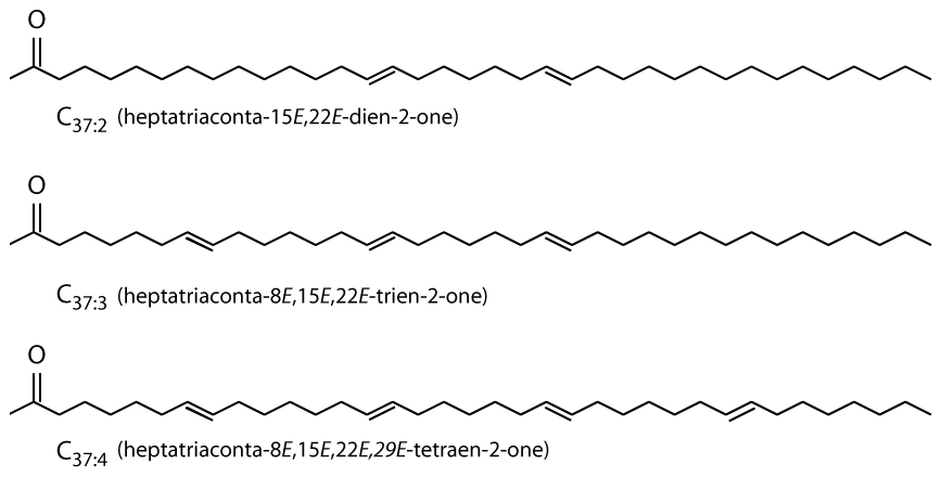
Figure 1Alkenones are C37 unsaturated methyl ketones (Brassell et al., 1986; Rechka and Maxwell, 1987).
The enzyme carbonic anhydrase (CA) can catalyse the dehydration of to [CO2](aq) to speed up availability of carbon if the [CO2](aq) reservoir is depleted and has been observed in several haptophytes, including coccolithophores (Rost et al., 2003; Riebesell et al., 2007). The exact contribution of CA remains unclear, but two possible mechanisms for CCMs have been postulated (Reinfelder, 2011): (1) CA catalyses dehydration of at the cell surface, which then allows increased CO2 to diffuse into the cell passively, and (2) is transported into the cell and then converted by CA. Both of these options will likely impact the proxy, firstly by changing the effective [CO2](aq) within the cell (and so impacting εp) and secondly by imparting another carbon isotopic fractionation during CA catalysation which is not considered by the proxy system. However CA activity in coccolithophores does not appear to be regulated by CO2 as it is in diatoms and Phaeocystis (Rost et al., 2003), which may indicate a less-well-developed CCM in coccolithophores.
Calcifying coccolithophores (which include alkenone producers E. huxleyi and G. oceanica) may be able to utilize directly as a carbon source (Trimborn et al., 2007), with precipitation of CaCO3 providing an acid for the dehydration of , but this still requires sufficient entering the cell, and it is unclear whether calcification aids DIC acquisition (Riebesell et al., 2000; Zondervan et al., 2002). The light-dependent leak of carbon (as CO2 and DIC) back from haptophyte cells (including the coccolithophore E. huxleyi) to seawater (Tchernov et al., 2003) suggests that CCMs are energy intensive and can concentrate DIC within the cell. Even with active CCMs, it appears that in the ocean coccolithophores are CO2 limited under some circumstances (Riebesell et al., 2007).
Calculating CO2 from alkenone δ13C values: the proxy
In this study I use the now large number of published records which overlap with ice core records of atmospheric CO2 concentration (Tables 1 and 2) to explore the relationship between and CCMs in the Pleistocene, where our understanding of atmospheric CO2 concentration is best.
Multiple records of have been published for the Pleistocene (Fig. 2, Table 1), allowing direct comparison with ice-core-based CO2 records (Table 2). These records are globally distributed in longitude but are concentrated at low-latitude sites, largely as there is a general preference for sites which have (in the modern ocean) surface waters close to equilibrium with the atmosphere (Fig. 2, Table 1). In longer-term palaeoclimate studies there has also been a preference for low-latitude gyre sites in the belief that these sites are more likely to be oceanographically stable over long time intervals (Pagani et al., 1999). Most of the records included here (Table 1, Fig. 2) were generated with the aim to reconstruct atmospheric CO2 concentration; however one, the MANOP Site C of Jasper et al. (1994), was used to explicitly reconstruct changing disequilibrium due to oceanographic frontal changes over time and so is excluded from the following analysis.
Bae et al. (2015)Jasper and Hayes (1990)Palmer et al. (2010)Badger et al. (2019)Zhang et al. (2013)Jasper et al. (1994)Andersen et al. (1999)Table 1Sites with Pleistocene records. Note that the MANOP Site C record was generated to track changes in surface water–atmosphere equilibrium, not atmospheric pCO2, so, although it is included here for completeness, it is not included in the analysis. Distance from the coast is calculated from the intermediate-resolution version of GSHHG and computed using Generic Mapping Tools (Wessel and Smith, 1996; Wessel et al., 2019).

The full record for ODP Site 925 extends to 38.62 Ma.
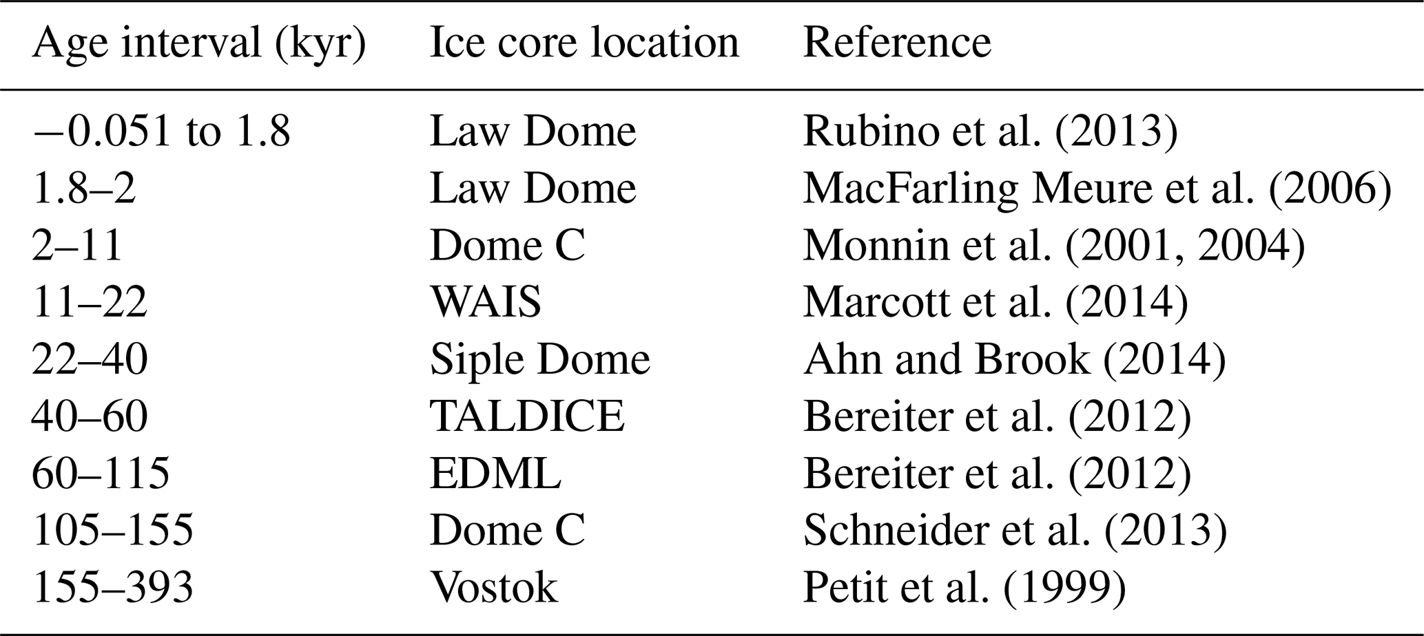
Table 2Sources of ice core data, as compiled by Bereiter et al. (2015). WAIS – West Antarctic Ice Sheet; TALDICE – TALos Dome Ice CorE; and EDML – EPICA Dronning Maud Land. Age given as gas age relative to 1950.
Whilst these sites do only span a relatively small latitudinal extent, the diversity of settings does allow for investigation of any secondary controls on alkenone δ13C values (δ13Calkenone) – in particular, differences in oceanographic setting and SST to test the hypothesis that low [CO2](aq) breaks the relationship between δ13Calkenone and atmospheric CO2 concentration, as might be expected if haptophytes are able to actively take up carbon from seawater to meet metabolic demand (i.e. activate CCMs).
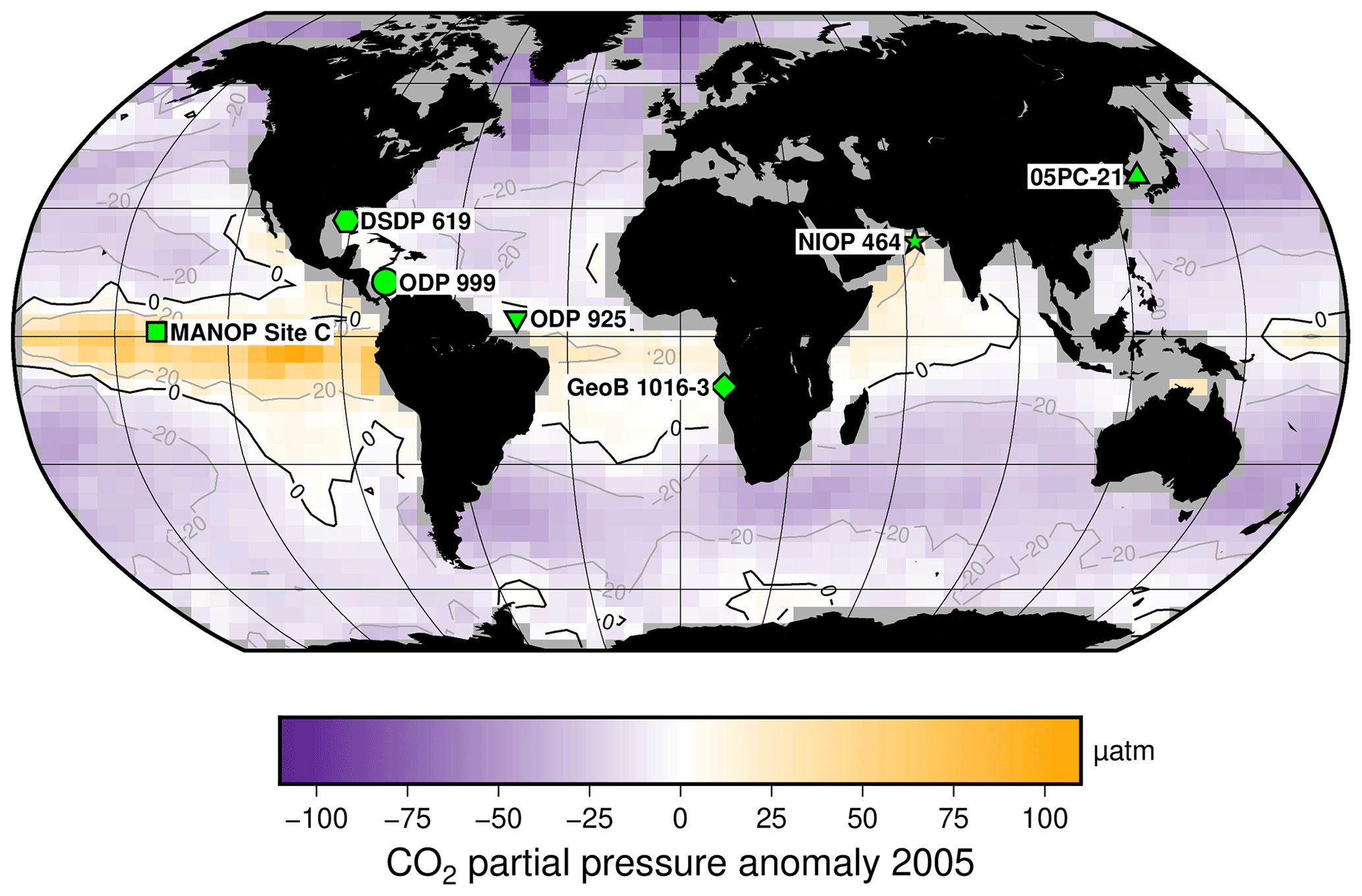
Figure 2Study sites relative to mean annual surface ocean CO2 disequilibrium for 2005. Sites are globally distributed in longitude but restricted in latitude, as generally sites are chosen to be close to surface water equilibrium with the atmosphere. Sites used for this study are indicated, over the mean annual surface ocean disequilibrium for 2005 calculated from Takahashi et al. (2014). The MANOP Site C (Jasper et al., 1994) was chosen to study the disequilibrium at that site, so it is shown here but not used in the following analyses. Site symbols are used throughout the figures: ODP 999 – circle; 05PC-21 – triangle; ODP 925 – inverted triangle; DSDP 619 – hexagon; MANOP Site C – square; NIOP 464 – star; and GeoB 1016-3 – diamond.
To facilitate fair comparison between sites and consistent comparison with the ice core records, all records were recalculated using a consistent approach. The approach is based on Bidigare et al. (1997), which updated the initial approach of Jasper and Hayes (1990) to . This approach removes some additional corrections used in the original publication of the records (such as growth rate adjustment for NIOP 464; Palmer et al., 2010) but does allow for direct comparison to be made. For all sites the “b” term was estimated using modern-day surface (Bidigare et al., 1997; Pagani et al., 2009)
An overview of how data are typically generated is given in Badger et al. (2013b). Briefly, to calculate εp requires the stable carbon isotopic composition of the dissolved CO2 () and haptophyte biomass (δ13Corg). The isotopic fractionation between δ13Calkenone and δ13Corg is first corrected assuming a constant fractionation (εalkenone) of 4.2 ‰ (Garcia et al., 2013; Popp et al., 1998; Bidigare et al., 1997):
The isotopic composition of DIC is estimated using (ideally) the δ13C value of planktic foraminifera and the temperature-dependent fractionation between calcite and [CO2](g) experimentally determined by Romanek et al. (1992), where T is sea surface temperature in degrees Celsius (SST):
The value of the carbon isotopic composition of CO2(g) () can then be calculated:
From this can be calculated using the relationship experimentally determined by Mook et al. (1974),
and
Finally εp can be calculated:
and from that [CO2](aq) is calculated using the isotopic fractionation during carbon fixation (εf) and b, which represents the summation of physiological factors:
Here εf is assumed to be a constant 25 ‰ (Bidigare et al., 1997). In the modern ocean the b term, which accounts for physiological factors such as cell size and growth rate, shows a close correlation with (Bidigare et al., 1997; Pagani et al., 2009). However, the relationship between b, growth rate, and has recently been questioned (Zhang et al., 2019, 2020) but for the purposes of this analysis is assumed to hold. This is discussed further below. Values for SST, δ13Calkenone, δ13Ccarbonate, salinity, and are either taken from the original publications or estimated from modern ocean estimates (Takahashi et al., 2009; Antonov et al., 2010; Garcia et al., 2013; Locarnini et al., 2013).
Providing that the atmosphere is in equilibrium with surface water, the concentration of atmospheric CO2 can be calculated from [CO2](aq) (and vice versa if atmospheric CO2 concentration is known) using Henry's law:
The solubility coefficient (KH) is dependent on salinity and SST, and here it is calculated following the parameterization of Weiss (1970, 1974).
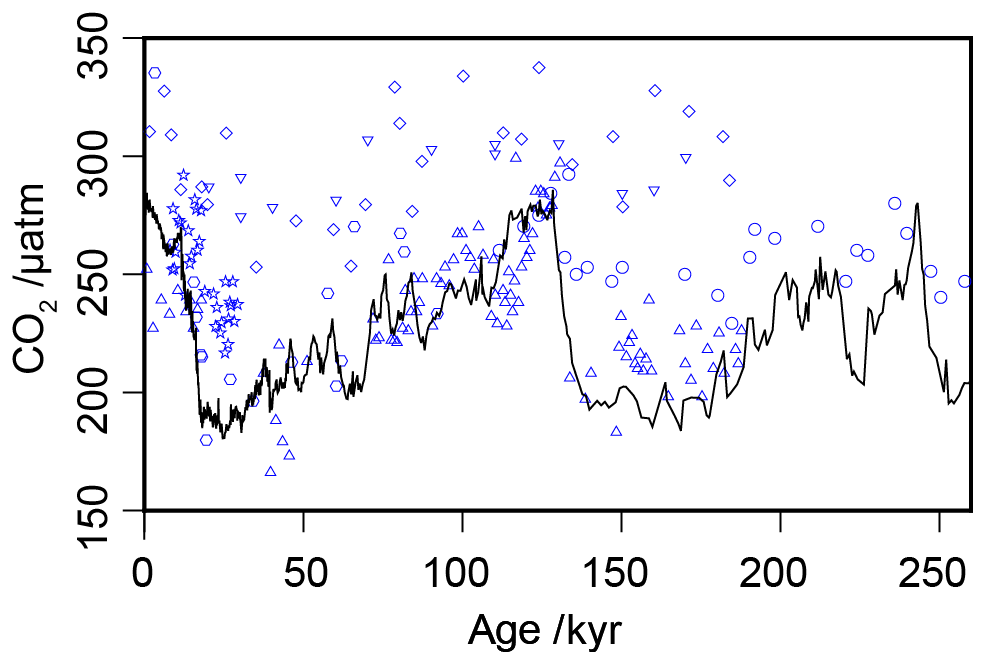
Figure 3Compiled -based estimates of atmospheric CO2 concentration over the past 260 kyr (blue circles), with the ice core compilation of Bereiter et al. (2015) shown as the solid black line. Full sources for the ice core and records are in Tables 1 and 2.
3.1 Multi-site comparisons between and the ice core records
Across the six sites included in this analysis, there are 217 -based estimates of atmospheric CO2 concentration over the past 260 kyr for comparison with the ice core records (Table 2; Bereiter et al., 2015). When all estimates are considered together over 260 kyr, this compilation of proxy-based records fails to replicate the ice core record (Fig. 3). This has already been noted at specific sites (e.g. Site 999 in the Caribbean; Badger et al., 2019), but this is the first time that all available records coincident with the Pleistocene ice core records have been compiled using a common methodology. Notably the -based estimates are rarely lower than time-equivalent ice core estimate, but frequently higher. Given that haptophytes require carbon to satisfy metabolic demand, this is perhaps unsurprising; if at times of low carbon availability haptophytes can switch from passive to active uptake to satisfy metabolic demand, it would be times of low atmospheric CO2 concentration (and so lower [CO2](aq)) when the active uptake is most likely to be needed. As -based estimates of atmospheric CO2 concentration rely on the assumption of a purely diffusive uptake of carbon, it is therefore likely that the proxy would perform worse at times of low atmospheric CO2 concentration.
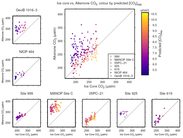
Figure 4Crossplots of -based atmospheric CO2 concentration (y axes) vs. the time-equivalent estimate from ice core records (x axes; Bereiter et al., 2015; Table 2). The large panel compiles all sites, with the exception of MANOP Site C, as explained in the text. Symbols are coloured by predicted [CO2](aq) for each site and time as explained in the text. Full sources for alkenone data are shown in Table 1. A 1:1 line is included in all plots for comparison.
The haptophytes do not directly interact with the atmosphere, obtaining their carbon from dissolved carbon. As it is not only atmospheric CO2 concentration which controls the concentration of dissolved carbon ([CO2](aq)) but also temperature, alkalinity, and other oceanographic factors which control the equilibrium state between surface waters at the atmosphere (Fig. 2), the multiple sites in different settings now give the opportunity to test whether other factors are important in controlling the accuracy of .
To produce time-equivalent estimates of atmospheric CO2 concentration for comparison with the ice core records, a simple linear interpolation of the Bereiter et al. (2015) compilation was initially used (Fig. 4). This assumes that both the age model of the ice core and the published age models of the sites are correct and equivalent. This is almost certainly not the case, and so for the calculations below, a ±3000 year uncertainty is included for ages of both the ice core and values. Figure 4 shows that -based atmospheric CO2 concentration agree with ice core CO2 at some sites and at some times, but not throughout. Sites 05-PC21 (Bae et al., 2015) and DSDP Site 619 (Jasper and Hayes, 1990) perform quite well throughout, whilst ODP Site 999 (Badger et al., 2019) and NIOP 464 (Palmer et al., 2010) only appear to agree at higher values of CO2, and at ODP Site 925 (Zhang et al., 2013) and GeoB 1016-3 (Andersen et al., 1999) there is very little overlap between the two methods of reconstructing atmospheric CO2 concentration.
To explore whether [CO2](aq) is an important influence on , I calculate predicted [CO2](aq) ([CO2](aq)−predicted) for each of the samples. To calculate [CO2](aq)−predicted, the time-equivalent value of atmospheric CO2 concentration from the ice core record is used in combination with Eq. (8) to calculate [CO2](aq) at the time of alkenone production for each sample. Reconstructed estimates of SST and salinity are used as for above, along with any estimated surface water–atmosphere disequilibrium. Points in Fig. 4 are then coloured by [CO2](aq)−predicted.
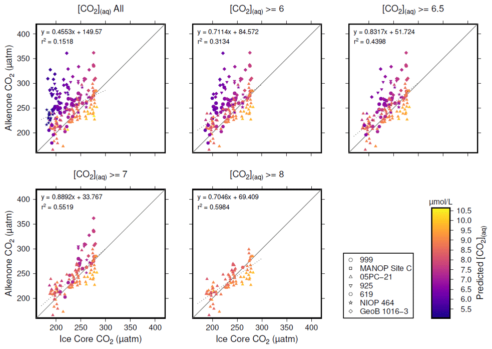
Figure 5Crossplots of -based atmospheric CO2 concentration (Table 1; y axes) vs. the time-equivalent estimate from ice core records (x axes; Bereiter et al., 2015; Table 2). The sample of published vales of was progressively restricted by [CO2](aq)−predicted, indicated by the subplot titles. Individual values are coloured by [CO2](aq)−predicted, and sites indicated by shape (see key). Coefficients of determination and equations of best fit are shown in each panel, along with a 1:1 line.
Inspection of Fig. 4 suggests a connection between ([CO2](aq)−predicted) and the skill of to reconstruct atmospheric CO2 concentration. The points clustering around the 1:1 line are lighter in colour (so with higher [CO2](aq)−predicted), whilst points falling away from the 1:1 line have lower [CO2](aq)−predicted. To explore this relationship, I progressively restricted the included samples on the basis of [CO2](aq)−predicted and at each stage calculated a Pearson correlation coefficient (r) and coefficient of determination (r2) for each subset. Under this analysis the correlation progressively increased as more of the low [CO2](aq)−predicted samples were excluded (Fig. 5). All analyses were performed in R (R Core Team, 2020) using RStudio (RStudio Team, 2020). This suggests that the fidelity of the depends on the concentration of [CO2](aq), improving at higher levels of [CO2](aq).
To further investigate this potential relationship, I progressively exclude samples based on [CO2](aq)−predicted with a step size of 0.05 µmol L−1, again calculating Pearson correlation coefficients and coefficients of determination between ice core and for each subsample of the population. The result is shown in Fig. 6. Here the analysis shows, similar to Fig. 5, that, as the samples with lowest [CO2](aq)−predicted are progressively removed, the correlation between ice core and increases. Furthermore, this continues only up until [CO2](aq)−predicted reaches 7 µmol L−1. Above this, the coefficient of determination plateaus, until the subsample reaches such a small size that spurious correlations become important (Fig. 6b).
3.2 Sensitivity and uncertainty tests
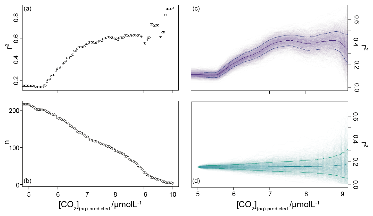
Figure 6Coefficient of determination (a) of a reducing sample of all compiled (Table 1) vs. the time-equivalent estimate from ice core records (Bereiter et al., 2015; Table 2). The sample reduces stepwise by 0.05 µmol L−1, and the number of records in each subsample is shown in panel (b). Panel (c) shows a 1000-member Monte Carlo analysis, whereby uncertainty in and age is considered, as detailed in the text. Panel (d) shows a similar 1000-member Monte Carlo analysis, but with random sampling of the whole population so that the number of samples is equivalent to the dataset shown in panel (c); i.e. the size of the sample follows that shown in panel (b). Means and 1σ uncertainties are shown as the bold lines.
It is possible that the pattern seen in Fig. 6b could emerge from a dataset shaped with increasing density surrounding the 1:1 correlation line without being driven by changes in [CO2](aq)−predicted. To explore this possibility, I ran a series of sensitivity experiments. In these, rather than reducing the sample by filtering by [CO2](aq)−predicted, the whole dataset (Table 1) was randomly ordered and then stepwise subsampled. To make this equivalent to the [CO2](aq)−predicted analysis above, I set the size of each subsample to be equal to each step in the original analysis. This produces a randomly selected but same-sized subsample such that the size of the subsample reduces in the same way as shown in Fig. 6b). Pearson correlation coefficients and coefficients of determination were calculated for each subsample as above, and I repeated this 1000 times, with the order of each sample randomized each time.
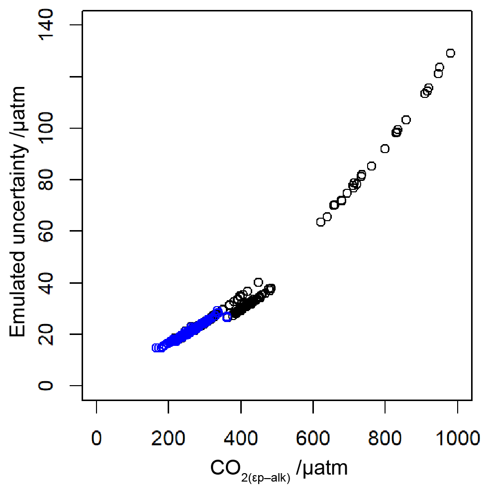
To allow for possible age model uncertainties, a 3000-year (1σ) uncertainty was also applied to each sample. This uncertainty was applied to the age of each sample prior to sampling of the ice core record, and it is applied as a normally distributed uncertainty. Uncertainty in measurements is typically calculated using Monte Carlo modelling of all the parameters (i.e. Pagani et al., 1999; Badger et al., 2013a, b); however this was not done in all the published work (Table 1), and some differences in approach were found across the published work. Therefore to create uncertainty estimates for each value in this study, I emulate the uncertainties based on the value. I built a simple emulator (Fig. 7) by running Monte Carlo uncertainty estimates for all of the included datasets (Table 1) using the same estimates of uncertainty for each variable in the calculation as applied in Badger et al. (2013a, b). This then allows the uncertainty to be included in the [CO2](aq)−predicted calculation as well as , and it allowed for uncertainty estimates to be site-ambivalent.
The result is shown in Fig. 6c and d, and it suggests that the 7 µmol L−1 break point remains valid. The absolute value of r2 is reduced, even at higher [CO2](aq)−predicted, but this would be expected given the addition of uncertainty in the age model, as the published age is most likely to align with the ice core. Given the rapid rate of change at deglaciations, this effect is likely to be particularly pronounced in this dataset as many records have high temporal resolution around deglaciations in order to attempt to resolve them. Any small age model offset introduced by the error modelling in these intervals also clearly has the potential to induce large differences between the and ice core values. Figure 6c and d clearly demonstrate that it is the filtering by [CO2](aq)−predicted rather than any spurious correlations which determines the shape of the data in Fig. 6a.
The plateau in r2 in Fig. 6a and c suggests that below a [CO2](aq)−predicted of ∼7 µmol L−1 is no longer as good a predictor of ice core CO2 as when [CO2](aq)−predicted > 7 µmol L−1. This is clear from comparing the relationship between samples where [CO2](aq)−predicted < 7 µmol L−1 with those where [CO2](aq)−predicted > 7 µmol L−1 in Fig. 8. Here the r2 for the former of 0.15 is substantially less than the latter of 0.55. I suggest that this is because below this threshold the fundamental assumption of , that carbon is passively taken up by haptophytes, no longer holds true. One obvious explanation for why this would be the case is that at low levels of [CO2](aq) haptophytes have to rely more on active uptake of carbon via CCMs in order to satisfy metabolic demand. Similar behaviour has been recognized in some culture studies (Laws et al., 1997, 2002; Cassar et al., 2006), with some evidence that the diatom Phaeodactylum tricornutum has a similar CCM threshold of 7 µmol L−1 (Laws et al., 1997). Whilst the evidence for the mechanism of CCM is poorer for coccolithophores than it is for diatoms, any CCM would be expected to compromise the proxy, either by increased supply of [CO2](aq) or by further carbon isotopic fractionation effects during carbon transport, or both (Stoll et al., 2019).
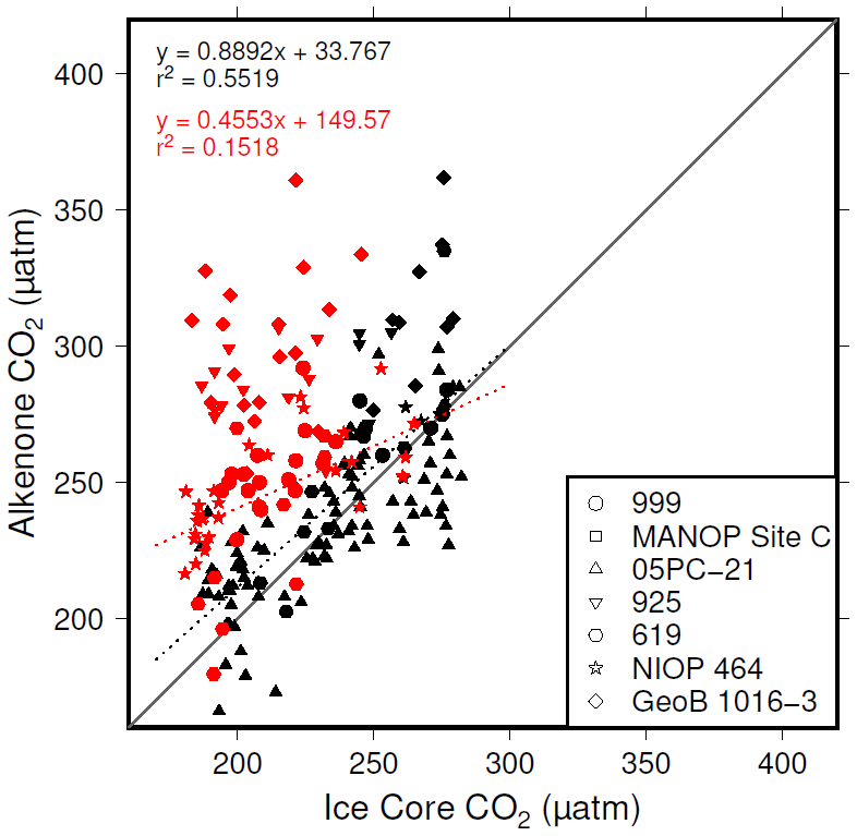
Figure 8Correlations between and ice core CO2, where [CO2](aq)−predicted > 7 µmol L−1 (black symbols) and [CO2](aq)−predicted < 7 µmol L−1 (red symbols).
By applying a threshold value for [CO2](aq)−predicted of 7 µmol L−1 to the published records (Table 1), values of which are influenced by active CCMs can be eliminated. Recognition of this new threshold value of [CO2](aq)−predicted allows for a new record of Pleistocene to be compiled. This compilation then much better replicates the glacial–interglacial pattern of CO2 change over the last 260 kyr (Fig. 9). Whilst this present compilation does rely on ice core CO2 records to estimate [CO2](aq)−predicted, and therefore has little direct utility as a CO2 record, it does demonstrate that recognition of a threshold response allows accurate CO2 reconstruction using . This may represent the point at which isotopic effects of CCMs (plausibly through increased CA activity or dehydration to meet C demand) overwhelm the assumptions of the proxy. This, as well as the behaviour shown in Fig. 6a and c, suggests that from the standpoint of the proxy CCMs may effectively be considered either active or not, and that when [CO2](aq) is plentiful passive uptake dominates, at least sufficiently in most oceanographic settings that can accurately record atmospheric CO2 concentration. This implies that, if areas of the ocean (or intervals of time) with low [CO2](aq) can be avoided, accurate reconstructions of atmospheric CO2 concentration can be acquired using .
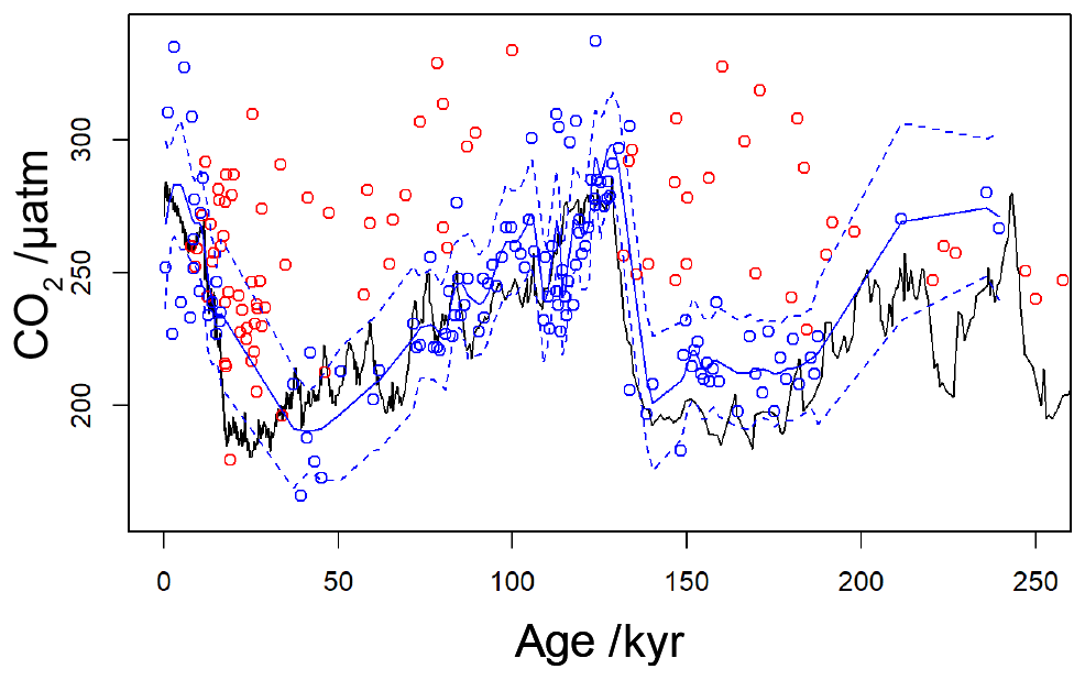
Figure 9Revised compilation of Pleistocene vs. ice core records. The compiled published records (Table 1) are shown as circles, coloured red where [CO2](aq)−predicted is below a threshold of 7 µmol−1 and blue where [CO2](aq)−predicted > 7 µmol−1. The solid blue line is a loess filter (span 0.1) through the [CO2](aq)−predicted > 7 µmol−1 values, with 95 % confidence intervals (dashed blue line). The black line is the ice core compilation of Bereiter et al. (2015) (Table 2).
As [CO2](aq) is affected by both SST via the temperature dependance of the Henry's law constant and atmospheric CO2 concentration, for to be effective in reconstructing atmospheric CO2 concentration, areas of warm water (i.e. tropical or shallow shelf regions) under relatively low atmospheric CO2 concentration must be avoided. However, as the atmospheric CO2 control renders the global surface ocean sufficiently replete with [CO2](aq) at Pliocene-like levels of atmospheric CO2 concentration and above (Martínez-Botí et al., 2015) at all but the warmest surface ocean temperatures, is likely to be a reliable system for most of the Cenozoic. It is only in the Pleistocene that atmospheric CO2 concentration is low enough for CCMs to be widely active across the surface ocean, with the low-CO2 glacials providing the most difficulty (Badger et al., 2019). This finding aligns well with evidence that CCMs developed in coccolithophores as a response to declining atmospheric CO2 concentration through the Cenozoic and were developing in [CO2](aq)-limited parts of the ocean in the late Miocene at the earliest, and likely not widespread until the Plio-Pleistocene (Bolton et al., 2012; Bolton and Stoll, 2013).
There have been recent attempts to correct for CCMs in -based reconstructions of atmospheric CO2 concentrations (Zhang et al., 2019; Stoll et al., 2019; Zhang et al., 2020). However, these assume that CCMs are always active and crucially do not fundamentally break the relationship between εp values and atmospheric CO2 concentration. However if this is not the case, and the relationship between εp values and atmospheric CO2 concentration fails at Pleistocene levels of atmospheric CO2, then Pleistocene records cannot be used to develop corrections of to be applied throughout the Cenozoic. If, as suggested by the analyses presented here, CCMs only act at low [CO2](aq), and largely only in conditions prevalent throughout the late Pliocene and Pleistocene, it is plausible that corrections based on Pleistocene records could overcompensate for CCMs in the rest of the Cenozoic, when the assumption of passive carbon uptake inherent in as traditionally applied may still be valid.
Reconstructions of past atmospheric CO2 concentration with proxy tools like are critical for understanding how the Earth's climate system operates, as long as the tools used can be relied upon to be accurate and precise. This re-analysis of existing Pleistocene records reveals that below a critical threshold of [CO2](aq) of 7 µmol−1 the relationship between δ13Calkenone and atmospheric CO2 concentration breaks down, plausibly because below this threshold haptophytes are able to actively take up carbon using CCMs in order to satisfy metabolic demand.
Although reconstructing the low levels of atmospheric CO2 concentration in the Pleistocene glacials and areas of the global ocean where [CO2](aq) is less than 7 µmol−1 will be impossible, for much of the Cenozoic the proxy retains utility. If care is taken to avoid regions and oceanographic settings where [CO2](aq) is expected to be abnormally low, remains an important and useful proxy to understand the Earth system.
This paper relies exclusively on previously published data, available with the original papers and in publicly available repositories. An R notebook supplement is available alongside this paper, along with data files, which allow full replication of all analyses performed.
The supplement related to this article is available online at: https://doi.org/10.5194/bg-18-1149-2021-supplement.
The author declares that there is no conflict of interest.
I am grateful to Gavin Foster and Tom Chalk for frequent and stimulating discussions on alkenone paleaobarometry. I thank all authors who made full datasets available online. I thank Kirsty Edgar for comments on various drafts and the two anonymous reviewers, whose comments greatly improved this paper.
Financial support for this work was provided by the School of Environment, Earth and Ecosystem Sciences, The Open University.
This paper was edited by Jack Middelburg and reviewed by two anonymous referees.
Ahn, J. and Brook, E. J.: Siple Dome ice reveals two modes of millennial CO2 change during the last ice age, Nat. Commun., 5, 3723, https://doi.org/10.1038/ncomms4723, 2014. a
Anagnostou, E., John, E. H., Edgar, K. M., Foster, G. L., Ridgwell, A., Inglis, G. N., Pancost, R. D., Lunt, D. J., and Pearson, P. N.: Changing atmospheric CO2 concentration was the primary driver of early Cenozoic climate, Nature, 533, 380–384, https://doi.org/10.1038/nature17423, 2016. a
Andersen, N., Müller, P. J., Kirst, G., and Schneider, R. R.: Alkenone δ13C as a Proxy for PastPCO2 in Surface Waters: Results from the Late Quaternary Angola Current, in: Use of Proxies in Paleoceanography, edited by: Fischer, G., and Wefer, G., Springer, Heidelberg, Berlin, Germany, 469–488, https://doi.org/10.1007/978-3-642-58646-0_19, 1999. a, b
Antonov, J. I., Seidov, D., Boyer, T. P., Locarnini, R. A., Mishonov, A. V., Garcia, H. E., Baranova, O. K., Zweng, M. M., and Johnson, D. R.: World Ocean Atlas 2009, Salinity, vol. 2, edited by: Levitus, S., US Government Printing Office, Washington DC, USA, NOAA Atlas NESDIS 69, 184 pp., 2010. a
Badger, M. P. S., Lear, C. H., Pancost, R. D., Foster, G. L., Bailey, T. R., Leng, M. J., and Abels, H. A.: CO2 drawdown following the middle Miocene expansion of the Antarctic Ice Sheet, Paleoceanography, 28, 42–53, https://doi.org/10.1002/palo.20015, 2013a. a, b, c, d
Badger, M. P. S., Schmidt, D. N., Mackensen, A., and Pancost, R. D.: High-resolution alkenone palaeobarometry indicates relatively stable pCO2 during the Pliocene (3.3–2.8 Ma), Philos. T. Roy. Soc. A, 371, 20130094, https://doi.org/10.1098/rsta.2013.0094, 2013b. a, b, c, d, e, f
Badger, M. P. S., Chalk, T. B., Foster, G. L., Bown, P. R., Gibbs, S. J., Sexton, P. F., Schmidt, D. N., Pälike, H., Mackensen, A., and Pancost, R. D.: Insensitivity of alkenone carbon isotopes to atmospheric CO2 at low to moderate CO2 levels, Clim. Past, 15, 539–554, https://doi.org/10.5194/cp-15-539-2019, 2019. a, b, c, d, e, f
Bae, S. W., Lee, K. E., and Kim, K.: Use of carbon isotopic composition of alkenone as a CO2 proxy in the East Sea/Japan Sea, Cont. Shelf Res., 107, 24–32, https://doi.org/10.1016/j.csr.2015.07.010, 2015. a, b
Beerling, D. J. and Royer, D. L.: Convergent Cenozoic CO2 history, Nat. Geosci., 4, 418–420, https://doi.org/10.1038/ngeo1186, 2011. a
Bereiter, B., Lüthi, D., Siegrist, M., Schüpbach, S., Stocker, T. F., and Fischer, H.: Mode change of millennial CO2 variability during the last glacial cycle associated with a bipolar marine carbon seesaw, P. Natl. Acad. Sci. USA, 109, 9755–9760, https://doi.org/10.1073/pnas.1204069109, 2012. a, b
Bereiter, B., Eggleston, S., Schmitt, J., Nehrbass-Ahles, C., Stocker, T. F., Fischer, H., Kipfstuhl, S., and Chappellaz, J.: Revision of the EPICA Dome C CO2 record from 800 to 600 kyr before present, Geophys. Res. Lett., 42, 542–549, https://doi.org/10.1002/2014GL061957, 2015. a, b, c, d, e, f, g, h
Bidigare, R., Fluegge, A., Freeman, K. H., Hanson, K., Hayes, J. M., Hollander, D., Jasper, J. P., King, L. L., Laws, E. A., Milder, J., Millero, F. J., Pancost, R., Popp, B. N., Steinberg, P., and Wakeham, S. G.: Consistent fractionation of 13C in nature and in the laboratory: Growth-rate effects in some haptophyte algae, Global Biochem. Cy., 11, 279–292, 1997. a, b, c, d, e, f, g
Bolton, C. T. and Stoll, H. M.: Late Miocene threshold response of marine algae to carbon dioxide limitation, Nature, 500, 558–562, https://doi.org/10.1038/nature12448, 2013. a, b
Bolton, C. T., Stoll, H. M., and Mendez-Vicente, A.: Vital effects in coccolith calcite: Cenozoic climate-pCO2 drove the diversity of carbon acquisition strategies in coccolithophores?, Paleoceanography, 27, PA4204, https://doi.org/10.1029/2012PA002339, 2012. a, b, c
Brassell, S., Eglinton, G., and Marlowe, I.: Molecular stratigraphy: a new tool for climatic assessment, Nature, 320, 129–133, 1986. a, b, c
Cassar, N., Laws, E. A., and Popp, B. N.: Carbon isotopic fractionation by the marine diatom Phaeodactylum tricornutum under nutrient- and light-limited growth conditions, Geochim. Cosmochim. Ac., 70, 5323–5335, https://doi.org/10.1016/j.gca.2006.08.024, 2006. a, b
Conte, M. H., Volkman, J. K., and Eglinton, G.: Lipid biomarkers of the Haptophyta, in: The Haptophyte algae, edited by: Green, J. and Leadbeater, B., Oxford University Press, Oxford, UK, 351–377, 1994. a
Farrimond, P., Eglinton, G., and Brassell, S. C.: Alkenones in Cretaceous black shales, Blake-Bahama Basin, western North Atlantic, Org. Geochem., 10, 897–903, https://doi.org/10.1016/S0146-6380(86)80027-4, 1986. a
Foster, G. L., Lear, C. H., and Rae, J. W. B.: The evolution of pCO2, ice volume and climate during the middle Miocene, Earth Planet. Sc. Lett., 341–344, 243–254, https://doi.org/10.1016/j.epsl.2012.06.007, 2012. a
Foster, G. L., Royer, D. L., and Lunt, D. J.: Future climate forcing potentially without precedent in the last 420 million years, Nat. Commun., 8, 14845, https://doi.org/10.1038/ncomms14845, 2017. a
Garcia, H. E., Locarnini, R. A., Boyer, T. P., Antonov, J. I., Baranova, O. K., Zweng, M. M., Reagan, J. R., and Johnson, D. R.: World Ocean Atlas 2013, Dissolved Inorganic Nutrients (phosphate, nitrate, silicate), vol. 4, edited by: Levitus, S. and Mishonov, A., Tech. Rep., NOAA Atlas NESDIS 76, 25 pp., Silver Spring, MD, USA, 2014. a, b
Gradstein, F., Ogg, J., Schmitz, M., and Ogg, G.: The Geologic Time Scale 2012, 1st Edn., Elsevier, 1176 pp., https://doi.org/10.1016/C2011-1-08249-8, 2012. a
Jasper, J. and Hayes, J.: A carbon isotope record of CO2 levels during the late Quaternary, Nature, 347, 462–464, 1990. a, b, c
Jasper, J., Hayes, J., Mix, A., and Prahl, F.: Photosynthetic fractionation of 13C and concentrations of dissolved CO2 in the central equatorial Pacific during the last 255 000 years, Paleoceanography, 9, 781–798, 1994. a, b, c
Kürschner, W. M., Kvacek, Z., and Dilcher, D. L.: The impact of Miocene atmospheric carbon dioxide fluctuations on climate and the evolution, P. Natl. Acad. Sci. USA, 105, 449–453, 2008. a
Laws, E. A., Popp, B., Bidigare, R., Kennicutt, M., and Macko, S.: Dependence of phytoplankton carbon isotopic composition on growth rate and [CO2) aq: Theoretical considerations and experimental, Geochim. Cosmochim. Ac., 59, 1131–1138, 1995. a, b
Laws, E. A., Bidigare, R. R., and Popp, B. N.: Effect of growth rate and CO2 concentration on carbon isotopic fractionation by the marine diatom Phaeodactylum tricornutum, Limnol. Oceanogr., 42, 1552–1560, https://doi.org/10.4319/lo.1997.42.7.1552, 1997. a, b, c, d
Laws, E. A., Popp, B. N., Cassar, N., and Tanimoto, J.: 13C discrimination patterns in oceanic phytoplankton: likely influence of CO2 concentrating mechanisms, and implications for palaeoreconstructions, Funct. Plant Biol., 29, 323–333, https://doi.org/10.1071/Pp01183, 2002. a, b
Locarnini, R. A., Mishonov, A. V., Antonov, J. I., Boyer, T. P., Garcia, H. E., Baranova, O. K., Zweng, M. M., Paver, C. R., Reagan, J. R., Johnson, D. R., Hamilton, M., and Seidov, D.: World Ocean Atlas 2013, Temperature, vol. 1, edited by: Levitus, S. and Mishonov, A., Tech. Rep., NOAA Atlas NESDIS 73, 40 pp., Silver Springs, MD, USA, available at: https://www.nodc.noaa.gov/OC5/woa13/pubwoa13.html (last access: 12 February 2021), 2013. a
MacFarling Meure, C., Etheridge, D., Trudinger, C., Steele, P., Langenfelds, R., van Ommen, T., Smith, A., and Elkins, J.: Law Dome CO2, CH4 and N2O ice core records extended to 2000 years BP, Geophys. Res. Lett., 33, L14810, https://doi.org/10.1029/2006gl026152, 2006. a
Marcott, S. A., Bauska, T. K., Buizert, C., Steig, E. J., Rosen, J. L., Cuffey, K. M., Fudge, T. J., Severinghaus, J. P., Ahn, J., Kalk, M. L., McConnell, J. R., Sowers, T., Taylor, K. C., White, J. W. C., and Brook, E. J.: Centennial-scale changes in the global carbon cycle during the last deglaciation, Nature, 514, 616–619, 2014. a
Marlowe, I., Brassell, S., Eglinton, G., and Green, J.: Long-chain alkenones and alkyl alkenoates and the fossil coccolith record of marine sediments, Chem. Geol., 88, 349–375, https://doi.org/10.1016/0009-2541(90)90098-R, 1990. a
Martínez-Botí, M. A., Foster, G. L., Chalk, T. B., Rohling, E. J., Sexton, P. F., Lunt, D. J., Pancost, R. D., Badger, M. P. S., and Schmidt, D. N.: Plio-Pleistocene climate sensitivity evaluated using high-resolution CO2 records, Nature, 518, 49–54, https://doi.org/10.1038/nature14145, 2015. a, b, c
Monnin, E., Indermuhle, A., Dallenbach, A., Fluckiger, J., Stauffer, B., Stocker, T. F., Raynaud, D., and Barnola, J. M.: Atmospheric CO2 concentrations over the last glacial termination, Science, 291, 112–114, https://doi.org/10.1126/science.291.5501.112, 2001. a
Monnin, E., Steig, E. J., Siegenthaler, U., Kawamura, K., Schwander, J., Stauffer, B., Stocker, T. F., Morse, D. L., Barnola, J.-M., Bellier, B., Raynaud, D., and Fischer, H.: Evidence for substantial accumulation rate variability in Antarctica during the Holocene, through synchronization of CO2 in the Taylor Dome, Dome C and DML ice cores, Earth Planet. Sc. Lett., 224, 45–54, https://doi.org/10.1016/j.epsl.2004.05.007, 2004. a
Mook, W. G., Bommerson, J. C., and Staverman, W. H.: Carbon isotope fractionation between dissolved bicarbonate and gaseous carbon dioxide, Earth Planet. Sc. Lett., 22, 169–176, https://doi.org/10.1016/0012-821X(74)90078-8, 1974. a
Pagani, M., Freeman, K., and Arthur, M.: Late Miocene atmospheric CO2 concentrations and the expansion of C4 grasses, Science, 285, 876–879, 1999. a, b, c
Pagani, M., Zachos, J. C., Freeman, K. H., Tipple, B., and Bohaty, S.: Marked decline in atmospheric carbon dioxide concentrations during the Paleogene, Science, 309, 600–603, https://doi.org/10.1126/science.1110063, 2005. a
Pagani, M., Liu, Z., La Riviere, J., and Ravelo, A. C.: High Earth-system climate sensitivity determined from Pliocene carbon dioxide concentrations, Nat. Geosci., 3, 27–30, https://doi.org/10.1038/ngeo724, 2009. a, b, c, d
Pagani, M., Huber, M., Liu, Z., Bohaty, S. M., Henderiks, J., Sijp, W., Krishnan, S., and De Conto, R. M.: The role of carbon dioxide during the onset of Antarctic glaciation, Science, 334, 1261–1264, https://doi.org/10.1126/science.1203909, 2011. a
Palmer, M. R., Brummer, G. J., Cooper, M. J., Elderfield, H., Greaves, M. J., Reichart, G. J., Schouten, S., and Yu, J. M.: Multi-proxy reconstruction of surface water pCO2 in the northern Arabian Sea since 29 ka, Earth Planet. Sc. Lett., 295, 49–57, https://doi.org/10.1016/j.epsl.2010.03.023, 2010. a, b, c
Pearson, P. N., Foster, G. L., and Wade, B. S.: Atmospheric carbon dioxide through the Eocene-Oligocene climate transition, Nature, 461, 1110–1113, https://doi.org/10.1038/nature08447, 2009. a
Petit, J. R., Jouzel, J., Raynaud, D., Barkov, N. I., Barnola, J.-M., Basile, I., Bender, M., Chappellaz, J., Davis, M., Delaygue, G., Delmotte, M., Kotlyakov, V. M., Legrand, M., Lipenkov, V. Y., Lorius, C., Pepin, K., Ritz, C., Saltzman, E., and Stievenard, M.: Climate and atmospheric history of the past 420 000 years from the Vostok ice core, Antarctica, Nature, 399, 429–436, 1999. a
Popp, B., Laws, E. A., Bidigare, R., Dore, J., Hanson, K., and Wakeham, S. G.: Effect of phytoplankton cell geometry on carbon isotopic fractionation, Geochim. Cosmochim. Ac., 62, 67–77, 1998. a
R Core Team: A language and environment for statistical computing, available at: https://www.r-project.org/ (last access: 9 October 2020), 2020. a
R Studio Team: Integrated Development for R, RStudio, PBC, Boston, MA, USA, available at: http://www.rstudio.com/, last access: 18 September 2020. a
Raffi, I., Backman, J., Fornaciari, E., Pälike, H., Rio, D., Lourens, L., and Hilgen, F.: A review of calcareous nannofossil astrobiochronology encompassing the past 25 million years, Quaternary Sci. Rev., 25, 3113–3137, https://doi.org/10.1016/j.quascirev.2006.07.007, 2006. a
Rechka, J. and Maxwell, J.: Characterisation of alkenone temperature indicators in sediments and organisms, Org. Geochem., 13, 727–734, 1987. a, b
Reinfelder, J. R.: Carbon concentrating mechanisms in eukaryotic marine phytoplankton, Annu. Rev. Mar. Sci., 3, 291–315, https://doi.org/10.1146/annurev-marine-120709-142720, 2011. a, b
Riebesell, U., Revill, A. T., Holdsworth, D. G., and Volkman, J. K.: The effects of varying CO2 concentration on lipid composition and carbon isotope fractionation in Emiliania huxleyi, Geochim. Cosmochim. Ac., 64, 4179–4192, https://doi.org/10.1016/S0016-7037(00)00474-9, 2000. a
Riebesell, U., Schulz, K. G., Bellerby, R. G., Botros, M., Fritsche, P., Meyerhöfer, M., Neill, C., Nondal, G., Oschlies, A., Wohlers, J., and Zöllner, E.: Enhanced biological carbon consumption in a high CO2 ocean, Nature, 450, 545–548, https://doi.org/10.1038/nature06267, 2007. a, b
Romanek, C. S., Grossman, E. L., and Morse, J. W.: Carbon isotopic fractionation in synthetic aragonite and calcite: Effects of temperature and precipitation rate, Geochim. Cosmochim. Ac., 56, 419–430, https://doi.org/10.1016/0016-7037(92)90142-6, 1992. a
Rost, B., Riebesell, U., Burkhardt, S., and Sültemeyer, D.: Carbon acquisition of bloom-forming marine phytoplankton, Limnol. Oceanogr., 48, 55–67, https://doi.org/10.4319/lo.2003.48.1.0055, 2003. a, b
Rubino, M., Etheridge, D. M., Trudinger, C. M., Allison, C. E., Battle, M. O., Langenfelds, R. L., Steele, L. P., Curran, M., Bender, M., White, J. W. C., Jenk, T. M., Blunier, T., and Francey, R. J.: A revised 1000 year atmospheric δ13C-CO2 record from Law Dome and South Pole, Antarctica, J. Geophys. Res.-Atmos., 118, 8482–8499, https://doi.org/10.1002/jgrd.50668, 2013. a
Schneider, R., Schmitt, J., Köhler, P., Joos, F., and Fischer, H.: A reconstruction of atmospheric carbon dioxide and its stable carbon isotopic composition from the penultimate glacial maximum to the last glacial inception, Clim. Past, 9, 2507–2523, https://doi.org/10.5194/cp-9-2507-2013, 2013. a
Sosdian, S. M., Greenop, R., Hain, M. P., Foster, G. L., Pearson, P. N., and Lear, C. H.: Constraining the evolution of Neogene ocean carbonate chemistry using the boron isotope pH proxy, Earth Planet. Sc. Lett., 498, 362–376, https://doi.org/10.1016/j.epsl.2018.06.017, 2018. a
Stoll, H. M., Guitian, J., Hernandez-Almeida, I., Mejia, L. M., Phelps, S., Polissar, P., Rosenthal, Y., Zhang, H., and Ziveri, P.: Upregulation of phytoplankton carbon concentrating mechanisms during low CO2 glacial periods and implications for the phytoplankton pCO2 proxy, Quaternary Sci. Rev., 208, 1–20, https://doi.org/10.1016/j.quascirev.2019.01.012, 2019. a, b, c
Super, J. R., Thomas, E., Pagani, M., Huber, M., Brien, C. O., and Hull, P. M.: North Atlantic temperature and pCO2 coupling in the early-middle Miocene, Geology, 46, 519–522, https://doi.org/10.1130/G40228.1, 2018. a, b
Takahashi, T., Sutherland, S. C., Wanninkhof, R., Sweeney, C., Feely, R. A., Chipman, D. W., Hales, B., Friederich, G., Chavez, F., Sabine, C., Watson, A., Bakker, D. C. E., Schuster, U., Metzl, N., Yoshikawa-Inoue, H., Ishii, M., Midorikawa, T., Nojiri, Y., Körtzinger, A., Steinhoff, T., Hoppema, M., Olafsson, J., Arnarson, T. S., Tilbrook, B., Johannessen, T., Olsen, A., Bellerby, R., Wong, C. S., Delille, B., Bates, N. R., and de Baar, H. J. W.: Climatological mean and decadal change in surface ocean pCO2, and net sea–air CO2 flux over the global oceans, Deep-Sea Res. Pt. II, 56, 554–577, https://doi.org/10.1016/j.dsr2.2008.12.009, 2009. a
Takahashi, T., Sutherland, S. C., Chipman, D. W., Goddard, J., Newberber, T., and Sweeney, C.: Climatological Distributions of pH, pCO2, Total CO2, Alkalinity, and CaCO3 Saturation in the Global Surface Ocean, Carbon Dioxide Information Analysis Center, Oak Ridge National Laboratory, US Department of Energy, Oak Ridge, Tennessee, ORNL/CDIAC-160, NDP-094, https://doi.org/10.3334/CDIAC/OTG.NDP094, 2014. a
Tchernov, D., Silverman, J., Luz, B., Reinhold, L., and Kaplan, A.: Massive light-dependent cycling of inorganic carbon between oxygenic photosynthetic microorganisms and their surroundings, Photosynth. Res., 77, 95–103, https://doi.org/10.1023/A:1025869600935, 2003. a
Trimborn, S., Langer, G., and Rost, B.: Effect of varying calcium concentrations and light intensities on calcification and photosynthesis in Emiliania huxleyi, Limnol. Oceanogr., 52, 2285–2293, https://doi.org/10.4319/lo.2007.52.5.2285, 2007. a
Volkman, J. K.: Ecological and environmental factors affecting alkenone distributions in seawater and sediments, Geochem. Geophy. Geosy., 1, 1036, https://doi.org/10.1029/2000GC000061, 2000. a
Weiss, R. F.: The solubility of nitrogen, oxygen and argon in water and seawater, Deep-Sea Res. Pt. I, 17, 721–735, https://doi.org/10.1016/0011-7471(70)90037-9, 1970. a
Weiss, R. F.: Carbon dioxide in water and seawater: the solubility of a non-ideal gas, Mar. Chem., 2, 203–215, 1974. a
Wessel, P. and Smith, W. H. F.: A global, self-consistent, hierarchical, high-resolution shoreline database, J. Geophys. Res.-Sol. Ea., 101, 8741–8743, https://doi.org/10.1029/96JB00104, 1996. a
Wessel, P., Luis, J. F., Uieda, L., Scharroo, R., Wobbe, F., Smith, W. H. F., and Tian, D.: The Generic Mapping Tools Version 6, Geochem. Geophy. Geosy., 20, 5556–5564, https://doi.org/10.1029/2019GC008515, 2019. a
Zhang, Y. G., Pagani, M., Liu, Z., Bohaty, S. M., and Deconto, R.: A 40 million year history of atmospheric CO2, Philos. T. Roy. Soc. A, 371, 20130096, https://doi.org/10.1098/rsta.2013.0096, 2013. a, b, c
Zhang, Y. G., Pearson, A., Benthien, A., Dong, L., Huybers, P., Liu, X., and Pagani, M.: Refining the alkenone-pCO2 method I: Lessons from the Quaternary glacial cycles, Geochim. Cosmochim. Ac., 260, 177–191, https://doi.org/10.1016/j.gca.2019.06.032, 2019. a, b, c
Zhang, Y. G., Henderiks, J., and Liu, X.: Refining the alkenone-pCO2 method II: Towards resolving the physiological parameter “b”, Geochim. Cosmochim. Ac., 281, 118–134, https://doi.org/10.1016/j.gca.2020.05.002, 2020. a, b, c
Zondervan, I., Rost, B., and Riebesell, U.: Effect of CO2 concentration on the ratio in the coccolithophore Emiliania huxleyi grown under light-limiting conditions and different daylengths, J. Exp. Mar. Biol. Ecol., 272, 55–70, https://doi.org/10.1016/S0022-0981(02)00037-0, 2002. a