the Creative Commons Attribution 4.0 License.
the Creative Commons Attribution 4.0 License.
 | 16 Feb 2021
Evaluating stream CO2 outgassing via drifting and anchored flux chambers in a controlled flume experiment
Filippo Vingiani
Nicola Durighetto
Marcus Klaus
Jakob Schelker
Thierry Labasque
Gianluca Botter
Carbon dioxide (CO2) emissions from running waters represent a key component of the global carbon cycle. However, quantifying CO2 fluxes across air–water boundaries remains challenging due to practical difficulties in the estimation of reach-scale standardized gas exchange velocities (k600) and water equilibrium concentrations. Whereas craft-made floating chambers supplied by internal CO2 sensors represent a promising technique to estimate CO2 fluxes from rivers, the existing literature lacks rigorous comparisons among differently designed chambers and deployment techniques. Moreover, as of now the uncertainty of k600 estimates from chamber data has not been evaluated. Here, these issues were addressed by analysing the results of a flume experiment carried out in the Summer of 2019 in the Lunzer:::Rinnen – Experimental Facility (Austria). During the experiment, 100 runs were performed using two different chamber designs (namely, a standard chamber and a flexible foil chamber with an external floating system and a flexible sealing) and two different deployment modes (drifting and anchored). The runs were performed using various combinations of discharge and channel slope, leading to variable turbulent kinetic energy dissipation rates ( m2 s−3). Estimates of gas exchange velocities were in line with the existing literature ( m2 s−3), with a general increase in k600 for larger turbulent kinetic energy dissipation rates. The flexible foil chamber gave consistent k600 patterns in response to changes in the slope and/or the flow rate. Moreover, acoustic Doppler velocimeter measurements indicated a limited increase in the turbulence induced by the flexible foil chamber on the flow field (22 % increase in ε, leading to a theoretical 5 % increase in k600). The uncertainty in the estimate of gas exchange velocities was then estimated using a generalized likelihood uncertainty estimation (GLUE) procedure. Overall, uncertainty in k600 was moderate to high, with enhanced uncertainty in high-energy set-ups. For the anchored mode, the standard deviations of k600 were between 1.6 and 8.2 m d−1, whereas significantly higher values were obtained in drifting mode. Interestingly, for the standard chamber the uncertainty was larger (+ 20 %) as compared to the flexible foil chamber. Our study suggests that a flexible foil design and the anchored deployment might be useful techniques to enhance the robustness and the accuracy of CO2 measurements in low-order streams. Furthermore, the study demonstrates the value of analytical and numerical tools in the identification of accurate estimations for gas exchange velocities. These findings have important implications for improving estimates of greenhouse gas emissions and reaeration rates in running waters.
- Article
(2713 KB) - Full-text XML
- BibTeX
- EndNote


Growing concerns about greenhouse gas emissions have increased the scientific interest in quantifying the role of inland waters in the global carbon cycle (Battin et al., 2009; Raymond et al., 2013; Hotchkiss et al., 2015; Marx et al., 2017). Most running waters are supersaturated in CO2 and are believed to be responsible for a globally large biogeochemical flux to the atmosphere occurring across air–water boundaries (Horgby et al., 2019; Hall and Ulseth, 2020). In particular, first-order streams are characterized by relatively high per-area CO2 evasion fluxes and cover a significant proportion of the global stream surface (Raymond et al., 2013; Schelker et al., 2016). Therefore, accurately quantifying air–water CO2 exchange in small headwater catchments is of paramount importance for global and regional assessments of CO2 emissions (Rawitch et al., 2019).
The gas flux across atmosphere–water interfaces (F) is commonly evaluated with Fick’s first law of diffusion (Wanninkhof et al., 2009):
where F is the CO2 flux (µmol s−1 m−2), k the gas exchange velocity (m s−1), Ce is the concentration in the water (µmol m−3), and C0 is the concentration in the water as if it was in equilibrium with the atmosphere (µmol m−3). According to Eq. (1), the flux of CO2 across the air–water interface (F) is directly proportional to the concentration gradient between the top and the bottom of the water boundary layer through a gas exchange velocity (k). Thus, assessing the value of k, which represents the depth of the water column that equilibrates with the atmosphere per unit time, is crucial for a correct estimation of F. The gas exchange velocity is an intrinsic surface-water characteristic difficult to measure (Schelker et al., 2016). Moreover, k can be strongly heterogeneous in space and time since it is linked to the near-surface turbulence that regulates the surface renewal rate in the mass boundary layer (MBL) (Zappa et al., 2003). For instance, Jeffrey et al. (2018) observed a 230-fold variation in the gas exchange velocity between two nearby stations along an estuary on the mid-coast of New South Wales, Australia. Likewise, Natchimuthu et al. (2017) estimated that flood events could produce a 7-fold increase in k in a hemiboreal catchment in southwestern Sweden. Within reach-scale model conceptualizations, measured k has been found to correlate with physical variables such as wind speed, flow velocity and channel slope (see Raymond et al., 2012, and references therein). These correlations led to empirical hydrogeomorphic equations that allow first-order k estimation for a given reach based on simple and measurable stream attributes. Further, these equations provide means to scale k across large geographic areas (Raymond et al., 2013). However, due to the inherent spatio-temporal heterogeneity of local hydraulic features, empirical laws might have limited predictability for specific case studies. In this context, independent estimates of k can be useful not only to validate these empirical models (Rawitch et al., 2019) or develop more accurate scaling equations (Ulseth et al., 2019), but also to get accurate k estimates for specific sites and field conditions. Such independent estimates of k can be obtained through a variety of direct or indirect methods (Hall and Ulseth, 2020), including the following: (i) gas tracer additions, such as propane and SF6; (ii) eddy covariance methods; (iii) analysis of temporal dynamics of dissolved gases; and (iv) floating chamber measurements.
The first applications of the floating chamber method for measuring stream–atmosphere gas exchange date back to the 1960s (Department of Scientific and Industrial Research, 1964). Traditionally, the change of gas concentration inside the chamber was measured by circulating chamber air through a gas analyser (e.g. Podgrajsek et al., 2013; Gålfalk et al., 2013) or by manually sampling chamber air at distinct times and then analysing the collected samples in the lab. Over the years, the chamber's design has been continuously improved. Recently, craft-made floating chambers supplied by internal CO2 sensors were proposed by Bastviken et al. (2015) as a promising technique to estimate CO2 fluxes. These chambers with internal CO2 sensors have since been frequently used and adapted to various applications (e.g. Lorke et al., 2015; Sawakuchi et al., 2017; Rosentreter et al., 2017; Jeffrey et al., 2018; Boodoo et al., 2019). The main advantages of floating chambers are their low cost, the easy-to-manage deployment and the flexibility of the chamber. Furthermore, chambers allow direct point measurements of gas fluxes, which are especially useful in headwater streams typically characterized by spatially heterogeneous conditions and complex CO2 patterns (Ploum et al., 2018; Rawitch et al., 2019). Floating chambers can be used either in drifting mode (i.e. the chamber is free to follow the current) or in anchored (a.k.a. stationary) mode (i.e. the chamber is fixed on a suitable support that prevents drifting). In running waters, floating chambers are preferably employed in the drifting mode (Alin et al., 2011; Beaulieu et al., 2012; Lorke et al., 2015), because anchored chambers can induce turbulence and enhance observed gas exchange rates across the water–atmosphere interface (Lorke et al., 2015). The applicability of the drifting deployment, however, is confined to low-surface-roughness flow systems, where the chamber is allowed to move downstream while maintaining the necessary stability.
Despite the recent spread of the use of chambers for quantifying CO2 fluxes from inland waters, the literature lacks rigorous comparisons among differently designed chambers and deployment techniques to address the problem of k misestimation due to chamber-induced turbulence. To date, only a few comparative studies exist (e.g. Vachon et al., 2010; Lorke et al., 2015), and all of them highlighted the need to better clarify the impact of chamber design on the reliability of k estimates. Furthermore, the uncertainty associated with k estimates relying exclusively on CO2 concentrations gathered using chamber-based CO2 measurements has been neither discussed nor quantified by previous studies. In the literature, the association of chamber-based estimates of k to specific flow conditions relies on simple averages among replicate experiments, and the inherent variability of k due to poor model structures or heterogeneous deployment modes is not accounted for. As errors in k propagate directly in the corresponding flux estimates, uncertainty in the estimates of gas exchange velocity can strongly limit our ability to investigate in-stream biogeochemical processes that rely on air–water CO2 exchange.
We pose the following two main research questions for this study: (1) is it possible to improve the reliability of k measurement by CO2 chambers through a novel chamber design, and (2) can we define a robust procedure to interpret the data derived from chamber experiments accounting for parameters uncertainty? Specifically, we focus on the usage of chamber methodology in an effort to (i) comparatively analyse the impact of chamber design improvements suggested by the recent literature (e.g. Sand-Jensen and Staehr, 2012; Lorke et al., 2015) and (ii) provide guidelines to interpret k values derived from chambers. By identifying novel procedures to analyse chamber data, we aim to offer useful tips to improve the robustness and reliability of chamber-based CO2 measurements in first-order streams.
2.1 Instrument
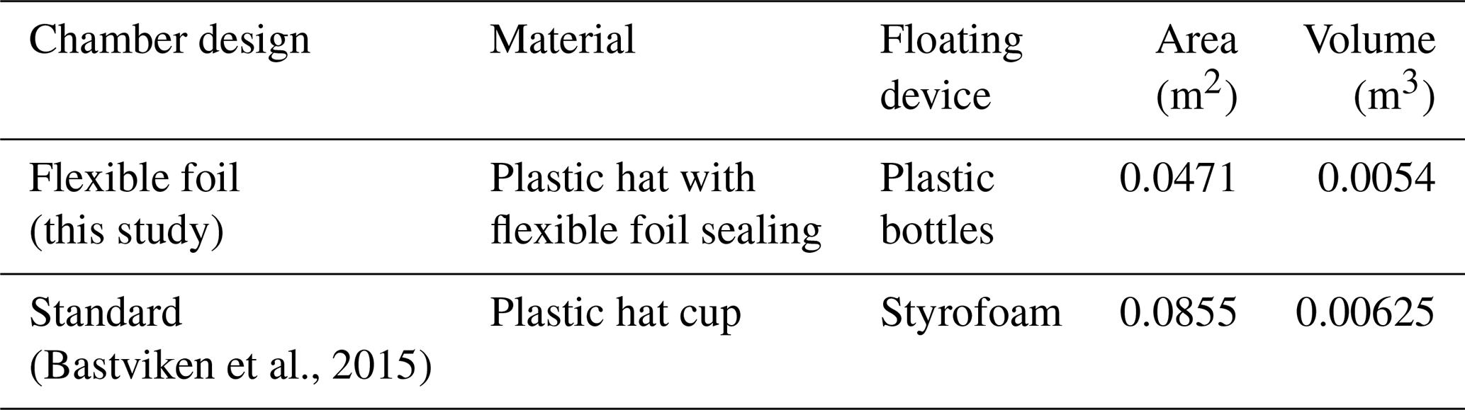
In this study, we used two different chamber designs, represented in Fig. 1. While neither chamber mounts a fan and both utilize the same internal CO2 logger, they differ in the sealing design. The chamber shown in Fig. 1a (hereafter “standard chamber”) is a traditional chamber with a rigid floating wall that guarantees the isolation of the air inside the chamber (Bastviken et al., 2015). The chamber shown in Fig. 1b (hereafter “flexible foil chamber”), instead, contains an external floating system and is equipped with a thin flexible sealing at the water surface. The polyethylene foil (plastic sheet UV4, Foliarex, Poznań, Poland) had a thickness of 150 µm and a height of 4 cm. The foil was mounted on the lower internal profile of the chamber cup. An adhesive tape (Extra Power Universal, Tesa, Hamburg, Germany) was used to fix the foil to the chamber and to guarantee the isolation of the air inside the chamber from the external atmosphere. The floating system (see Appendix C) was designed via three 0.5 L water bottles that were fixed on the external cup margin to sustain the rigid cup of the chamber above the water surface by about 2 cm (corresponding to half of the flexible foil height). The sealing was developed to reduce the turbulence induced by the chamber, especially when used in the anchored mode, as suggested by Lorke et al. (2015). A flexible foil sealing had been already utilized by Sand-Jensen and Staehr (2012). However, the sealing used by Sand-Jensen and Staehr (2012) was not complete, as it was implemented only in the direction of the water flow. A complete flexible sealing is particularly useful for drifting chambers that may rotate during drifting, and in turbulent flow fields where the dominant flow direction might be heterogeneous in space and time. Other geometrical characteristics of the two chambers are detailed in Table 1. The volume of the flexible foil chamber was computed taking into account the floating attitude of the chamber and the actual fraction of sealing foil below the channel surface.

Figure 1Two chamber designs: on (a) the standard chamber from Bastviken et al. (2015) and on (b) the flexible foil chamber (with a close-up of the peculiarity of the sealing).
Table 1Summary of the characteristics and geometrical properties of the two chambers.
The sensor (K33 ELG, SenseAir, Delsbo, Sweden) detects CO2 by non-dispersive infrared (NDIR) spectroscopy up to 10 000 ppm with a precision of ± 3 % of the measured value. Details on the sensor and its performance are given by Bastviken et al. (2015).
2.2 Study set-up
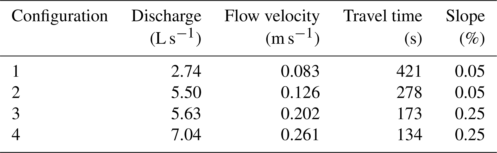
We performed a total of 100 experiments in the Lunzer:::Rinnen – Experimental Facility in Lunz am See, Austria. The flumes are fed by the Oberer Seebach and thus they are representative of a natural headwater stream. The flumes enabled the realization of a series of experiments without lateral input, in which important hydrogeomorphological factors (such as flow, velocity and slope) could be controlled. Measured data (air temperature and CO2 concentrations in the air and within the chamber) were collected with a variable frequency during each experiment's day depending on environmental and technical constraints. We performed a total of 55 drifting and 45 anchored chamber measurements. The data were collected using two different flumes at the Mesocosm facility. Both flumes were characterized by a gravel bed, and individual gravel stones had typical max and min axis lengths of 33 and 13 mm. Each flume was characterized by a distinct slope and was run with two different discharge configurations (Table ). Discharge was quantified using three different methods: salt injection, bucket and constant rate injection. For each experimental set-up, we carried out 1–5 slug injections, 5–10 bucket measurements and 2–12 constant rate injections. For the bucket method, we tracked the time needed to fill a 12.8 L bucket. For the slug and constant rate injection, we followed the protocols suggested by Moore (2004, 2005). In particular, we added a diluted salt tracer (NaCl+water) at the flume inlet and monitored electrical conductivity at intervals of 1 s (slug injection) or 30 s (constant rate injection) using loggers (HOBO U24, Onset, Bourne, MA, USA) placed 5 m downstream of the injection point and at the outlet. Constant rate injection was achieved by a peristaltic pump (Schlauchpumpe MV-GE, Ismatec, Wertheim, Germany). Next, we also measured the travel time in the flume system, calculated as the interval between the times when 50 % of the salt had passed the inlet and outlet loggers. Last, we computed the flow velocity (v) as the ratio between the distance between the inlet and outlet loggers (35 m) and the travel time. Elaborating the CO2 observations required the knowledge of the air atmospheric pressure (p); such data were derived from the meteorological station Lunz am See, located 300 m from the flumes.
Table 2Summary of the configuration set-up used at the EcoCatch flumes of the Lunz Mesocosm Infrastructure.
2.3 Sampling description
The sensors installed within the chambers recorded the time variability of CO2 concentration in the chamber volume during a run. The duration of each run was dependent on the underlying hydraulic conditions and the deployment mode. In the drifting mode, measurements were taken for a pre-defined maximum duration, which corresponds to the travel time of the chamber in the flume (see Table ). In the anchored mode the measurements lasted until near-equilibrium conditions were reached and typical incubation times were in the range of 10 to 50 min.
Time series of CO2 during each run were obtained with a measurement frequency of 30 s. To avoid biases in the saturation curves, it was important to aerate the chamber volume before placing the chamber above the stream and make a new run. It was observed that leaving the chamber aerated for 5 min prior to each run allowed the equilibrium between the chamber and the atmosphere to be reached. Accordingly, the selected procedure was to leave each chamber aerated for 10 min (2 times the estimated equilibrium time) before it was placed on the stream to make a new run. Despite this precaution, some of the measurements had to be discarded because the CO2 concentration in the chamber was not in equilibrium with the atmospheric value at the beginning of the run. Temperature inside the chamber was almost constant during the runs (less than 2.5 ∘C for more than 80 % of the runs). Regarding the calibration procedure in the field, we performed a post-process calibration referring to a constant CO2 concentration in the atmosphere equal to the reference value of 400 ppm for the entire experiment. This was necessary at times to eliminate long-term drifts of the sensors induced by the high humidity in the chamber air. Atmospheric CO2 concentrations were also monitored during the experiment with a sensor placed in the open air 3 m above the ground close to the flumes: the sensor measured atmospheric concentration close to 400 ppm.
2.4 Chamber-based estimates of mass transfer at the water–air interface
The gas flux across atmosphere–water interfaces (F) is here evaluated utilizing Eq. (1). Henry's law was used to get the water equilibrium concentration, Ce in Eq. (1), expressed as a function of the air concentration; the expression from Sander (2015) was employed to account for the dependence of Henry's constant (KH) on air temperature. Eq. (1) shows that k is a key parameter that governs the mass exchange across water–air interfaces. Two methods are available to estimate k from chamber measurements. Both methods are based on the definition of F at the air–water interface as the variation of the gas concentration inside the chamber per unit of time and area:
In Eq. (2), C′ is the concentration measured inside the floating chamber in (ppm = µmol mol−1), A is the exchange surface in (m2), and n is the number of moles in the air volume inside the floating chamber as per the gas law.
According to Eq. (2), the flux can be computed from the derivative of the chamber concentration in time. The first method (hereafter method 1) is based on the idea that if we select a sufficiently small interval (during which the exchange process is not influenced by the gas chamber concentration), the increments of concentration inside the chamber itself are linearly proportional to time; therefore, the flux remains constant and equal to the slope of the line interpolating the observed CO2 concentrations over time. In particular, the velocity k (in m s−1) can be computed as the ratio between the measured flux (Eq. 2) and the difference between the gas concentration in water, Ce, and the gas concentration in water as if it was in equilibrium with the atmosphere, C0:
Observations are fitted via a linear model and then the slope (i.e. ) is used to estimate k. The application of method 1 relies on the knowledge of the value of Ce, which is usually obtained from either direct or indirect measurements. However, Ce can also be obtained from the CO2 saturation curve provided by a steady floating chamber, i.e. from the saturation curve of a chamber allowed to reach near-equilibrium conditions as in Bastviken et al. (2015). Our estimates of k from the chamber employed with the drifting method use the Ce obtained from the steady chambers avoiding biases associated with the calibration of different instruments. To this aim, the mean Ce observed by simultaneously deployed steady chambers was used. During the experiment, we got at least one Ce measure for each drifting run in the range of 1 h, which was used for the interpretation of the chambers' data. Peter et al. (2014) showed that the natural diel variability of CO2 concentration in the stream feeding the flume is on average 375 ± 133 µatm per day in summer. In this work, a maximum variation of 100 ppm within 1 h for CO2 in stream water would result. Therefore, the estimates of k could be altered by 1.2 % at most.
An alternative method (method 2) is proposed here to interpret the results from steady deployments. According to Eq. (2), F can be also estimated as the derivative of the concentration's curve in time up to the achievement of near-equilibrium conditions between the water and the chamber's air. In this case, the decrease in F during the run is explicitly accounted for. The analytical solution of the differential equation that links the CO2 concentration inside the chamber and the CO2 concentration in the water (similar to Bastviken et al., 2004) is the following:
where = is the concentration in the chamber in (ppm) at time t0 ( ppm in this study), and is the concentration of CO2 in (ppm) in the chamber air as if the air inside the chamber was in equilibrium with water. k and are estimated by fitting (using a minimum least-square method) the exponential curve of Eq. (4) to the time series of CO2 observations in the chamber during a steady run. As for method 1, the assumption is that during the measurement the concentration of CO2 in the water below the chamber remains constant. Therefore, this assumption will gain more reliable results for short saturation curves. Given the maximum observed diel cycle of CO2 in the stream feeding the flumes (Peter et al., 2014), our assumption can be considered reasonable.
The main advantages of this method with respect to method 1 are twofold: (i) independent measures of Ce are not needed and (ii) the estimate of the gas exchange velocity is much more robust because it is calibrated over a larger set of observations. This method is best applied to cases in which a robust estimate of the equilibrium concentration is possible, e.g. because the full saturation curve is available, as for our steady deployments. Drifting deployments were analysed with method 1, whereas anchored deployments were analysed via method 2.
Regardless of the method used for k estimates, chamber concentration data were checked for quality after the experiment and some runs were discarded before the analysis. The retained runs fulfil the following requirements:
-
CO2 curves display an increasing monotonous trend during the whole run (visual test).
-
The saturation concentration in water must fall within a pre-defined reasonable range, 400 to 2000 ppm (e.g. Peter et al., 2014).
-
Nash–Sutcliffe efficiency (NSE) coefficients resulting from the model should be higher than 0.98, to avoid misestimate of k.
-
There should be at least 2 min of constant CO2 measurements prior to the beginning of each saturation curve; this ensures the chamber was in equilibrium with the atmosphere before the saturation curve was taken.
Before applying the check for data quality, some runs were discarded a priori because of missing data caused by technical problems with the chambers such as low battery voltage or accidental cable disconnections.
The analysis was carried out by standardizing k to a Schmidt number (Sc) of 600 (k600) via the commonly used expression for (see Appendix B). A total of 40 estimates of k600 were obtained with anchored (20) and drifting (20) deployments. The number of k600 estimates gathered through the standard chamber (28) largely exceeded the number of estimates from the flexible foil chamber (12); this was a result of the fact that three standard chambers but only one flexible foil chamber were used in the experiment.
2.5 Comparison with existing scaling laws
Our data were used to compare the observed dependence of k on the energy dissipation rate with two scaling relationships widely accepted in the literature. The first scaling law (SL1) was introduced by Zappa et al. (2003) whereas the second (SL2) was proposed by Ulseth et al. (2019). The relevant scaling laws are described in the following paragraphs.
According to the surface renewal theory, a continuous random renewal of the aqueous MBL with the bulk water below is observed due to turbulent eddies. Because the MBL is a thin layer at the air–water interface that governs the transport, the gas exchange is in turn influenced by hydrodynamic flow characteristics. This is quantified through the scaling equation SL1 as follows:
where 86 400 is a conversion factor from seconds to days, ν is the kinematic viscosity, α is an empirical coefficient, and ε is the turbulent kinetic energy (TKE) dissipation rate that was derived from the measurements of an acoustic Doppler velocity (ADV) meter (Vectrino+, down-looking probe, Nortek, Rud, Norway – see Appendix A). SL1 links k600 and ε via a power law relationship with an exponent of . We calibrated α via the least-square method based on the data derived from the deployment of the flexible foil and standard chambers via the steady method. Then the resulting values of α were compared with the range 0.16 to 0.43 observed in previous studies (Moog and Jirka, 1999; Zappa et al., 2007; Tokoro et al., 2008; Vachon et al., 2010).
The second scaling law used in this study (SL2) linearly correlates log(k600) and log(εemp), where εemp is the turbulent kinetic energy dissipation rate computed as the product between channel slope, flow velocity and gravitational acceleration. SL2 was empirically derived from the analysis of a large number of gas exchange velocities estimated from tracer gas additions over a wide range of streams worldwide (Ulseth et al., 2019). The analytical expression that links k600 and ϵemp is analogous to Eq. (5), but in this case the values of the slope and the intercept of the scaling law are 0.35 and 3.1, respectively.
2.6 Uncertainty analysis
The uncertainty in the estimate of gas-exchange velocity and equilibrium concentration via the exponential model was analysed using an informal Monte Carlo technique (i.e. generalized likelihood uncertainty estimation, GLUE; Beven and Binley, 1992). A random sample (one million) of couples (k and ) was generated from a bi-variate, bounded, uniform distribution and then the goodness of the exponential fitting was evaluated for each combination of parameters by means of the NSE. The range for NSE is : NSE = 1 corresponds to a perfect match of the model to the observed data, and NSE = 0 indicates that the model predictions are only as accurate as the mean of the observed data. Afterwards, only the couples of parameters providing satisfactory performance (i.e. NSE above a threshold value) were retained to derive the posterior bi-variate probability distribution of k and . This technique is widely employed in the analysis of the uncertainty of the parameters of hydrological models, but it has not been used previously in the context of CO2 studies. The method can be used to assess the uncertainty associated with the identification of model parameters via the fitting procedure of method 1 and 2, regardless of the chamber type (see Sect. 3.6).
3.1 Summary of water concentration and gas exchange velocity estimations
Stream CO2 concentrations were estimated based on CO2 data gathered through steady chambers (see Sect. 2.4, method 2). Estimated values during the whole experiment were in the range 555 to 1057 ppm, with a mean of 775 ppm and a standard deviation of 166 ppm. Regardless of the chamber type, measurements of from simultaneously deployed chambers exhibited a moderate variability; the mean coefficient of variation (cv) across different measurements, , was around 0.15. All measurements showed supersaturation of CO2 with respect to the atmosphere, thereby implying that during the deployment of the chambers the sensors recorded an increase in CO2 concentration over time (i.e. a positive flux from the stream to the atmosphere). General daily patterns of CO2 in the stream (Peter et al., 2014) were difficult to identify because of the limited chamber deployment frequency.
Overall, four different set-ups were analysed. Each set-up was characterized by a different combination of channel slope and discharge, thereby leading to a different value of εemp. Mean k600 for the four discharge and channel slope combinations ranged between 4.0 and 31.3 m d−1. To analyse the differences in k600 values from the standard and flexible foil chambers, we performed a two-sample t test assuming equal variances for the two groups (varSD and varFF) in accordance with Bonett's test (H0: varSD varFF = 1, p=0.79). The two-sample t test showed a higher mean k600 from the flexible foil chamber with respect to the standard chamber (H0: , p>0.97), particularly for high channel slopes. Moreover, k600 derived from flexible foil chambers had a smaller variability among replicated runs in the same configuration () with respect to the standard chambers (), even in cases where the number of replicates was similar. Gas exchange velocities derived from drifting and steady analysis showed a similar variability across the different set-ups, with a range of 4.7 to 31.3 and 4.0 to 27.8 m d−1 for the anchored and the drifting chamber, respectively. The range of values of εemp tested during the experiment covered 2 orders of magnitude (from about to m2 s−3). Overall, the corresponding estimates of k600 were in line with previous studies available from the literature for similar values of turbulent kinetic energy dissipation rates (Raymond et al., 2012; Schelker et al., 2016; Maurice et al., 2017). The impact of relevant physical properties of the flume, chamber type and deployment mode on k600 are discussed in the following sections.
Corresponding CO2 fluxes associated with each experiment were computed via Eq. (1) from the estimated values of k and Ce. Overall, CO2 fluxes were in the range 13–299 mmol m−2 d−1 with a mean value of 93 mmol m−2 d−1 and a cv of 0.67. Upper and lower limits of the above range were due to drifting deployments that showed the highest variability; measured fluxes had a mean of 93 mmol m−2 d−1 and a cv of 0.79, whereas measured fluxes for steady deployments were in the range 33 to 220 mmol m−2 d−1 with a mean of 87 mmol m−2 d−1 and a cv of 0.48.
3.2 Dependence of gas exchange velocity on slope and flow velocity
Least-square linear regression analysis of the observations obtained using the flexible foil chambers in steady mode suggested that the gas-exchange velocity increased with flow velocity (R2=0.84, n=7, p=0.004), in line with previous results (e.g. Raymond et al., 2012; Hall and Ulseth, 2020). In contrast, the standard chamber in anchored mode showed no significant relationship between flow velocity and k600 (R2=0.17, n=13, p=0.168). Instead, the interpretation of data from the drifting deployments was less straightforward. Data from the flexible foil chamber confirmed the trend observed in steady mode, even though the value of k600 relative to set-up 1 was unfortunately not measured (Table 3). In contrast, drifting data from the standard chamber showed a contrasting trend between k600 and v. In particular, k600 appeared to be unaffected by v for low channel slopes (set-up 1 vs. set-up 2) and inversely related to flow velocity for high channel slopes (set-up 3 vs. set-up 4).
The application of a least-square linear regression model to our observations from the flexible foil chamber, under both drifting and anchored modes, indicated a positive relationship between k600 and channel slope (drifting: R2=0.90, n=5, p=0.012; anchored: R2=0.73, n=7, p=0.015), in line with previous studies (e.g. Raymond et al., 2012; Lorke et al., 2019; Hall and Ulseth, 2020). On the contrary, the gas exchange velocities measured via the standard chamber did not provide a positive correlation between k600 and the channel slope, neither in drifting nor in anchored mode.
In conclusion, for the standard chamber we observed unexpected patterns of k600 for changing channel slopes and velocities, which were not in line with previous literature results. This might be an indication that the measurements taken using the flexible foil chamber were more reliable during our experiment.
Table 3Summary of ε, the mean and the coefficients of variation of the standardized gas exchange velocities, k600, observed during the different configurations in anchored and drifting deployments both for the standard (SD) and flexible foil (FF) chambers. The number between brackets in the column of the mean value indicates the number of measurements.
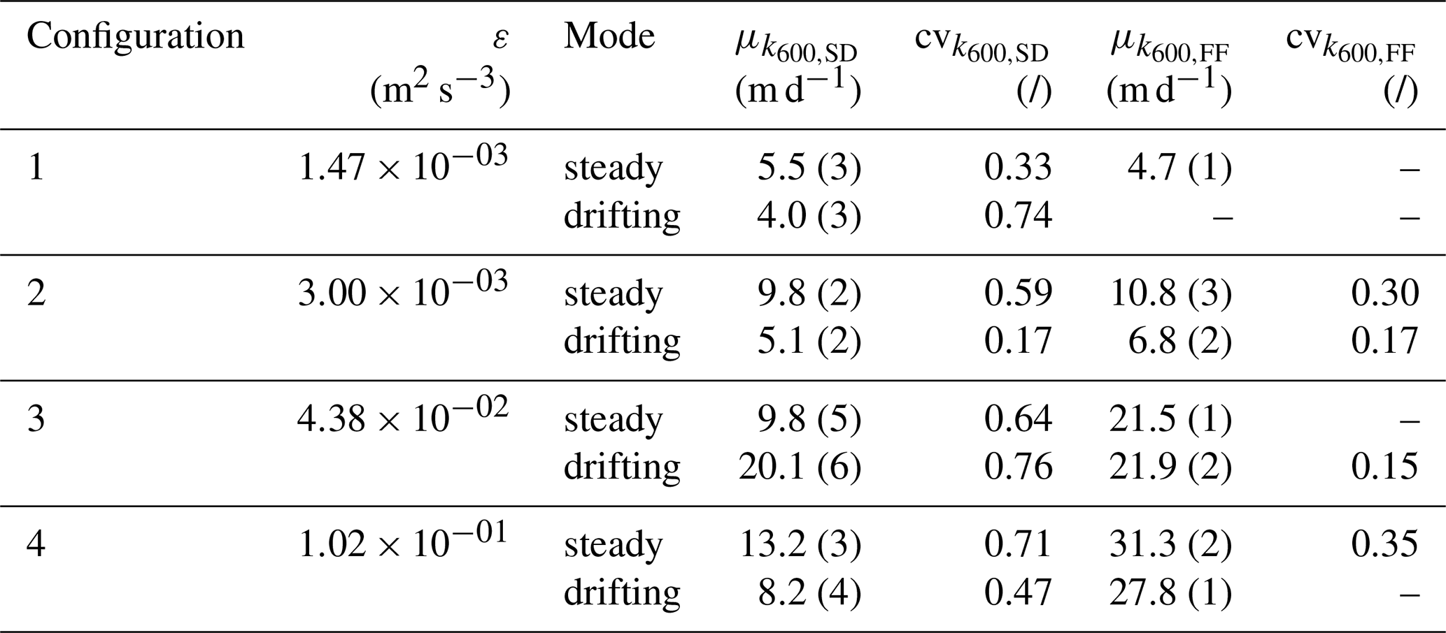
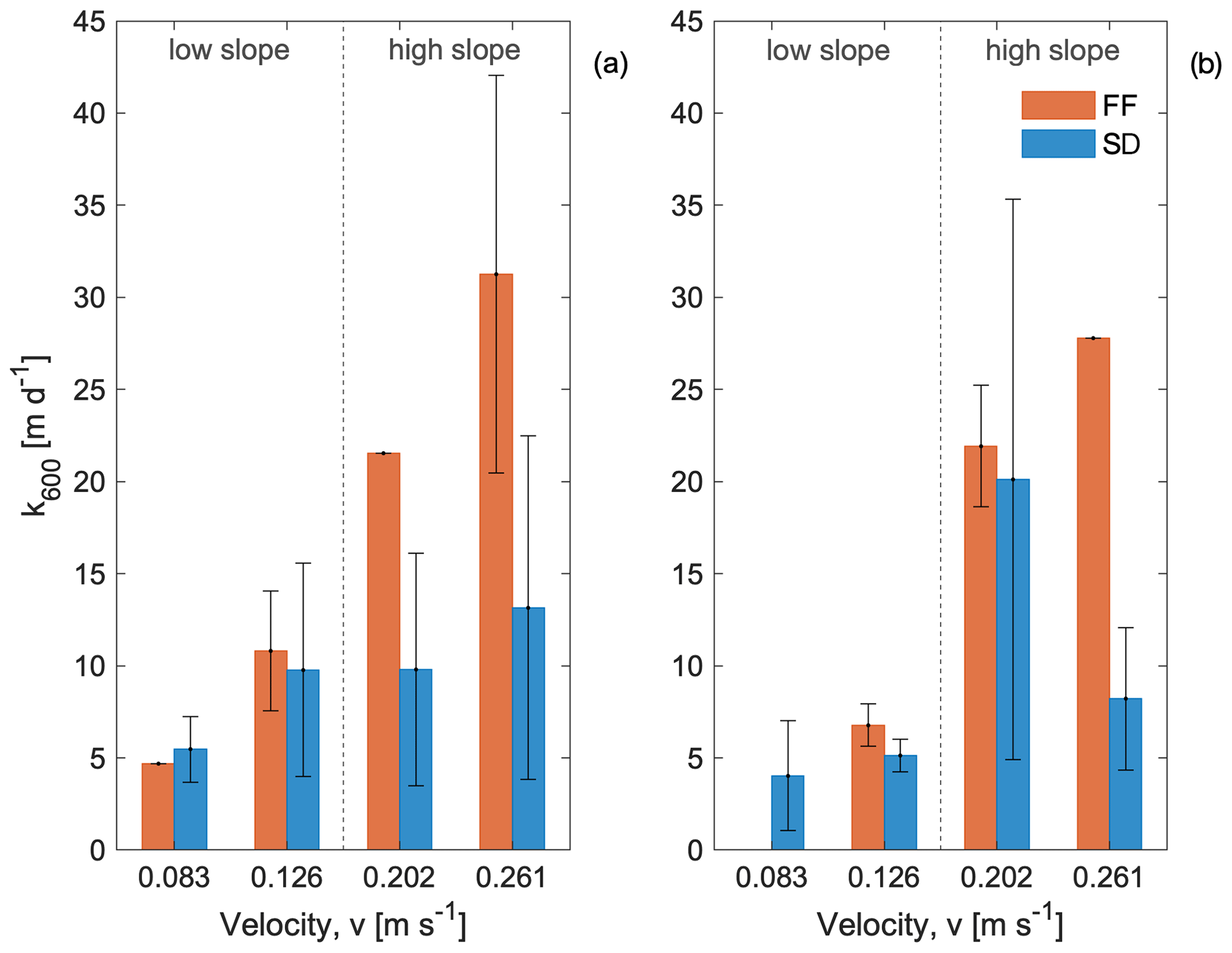
Figure 2Bar plot of the k600 values as a function of channel slope and flow velocity for steady (a) and drifting (b) modes. Error bars (standard deviations) are inserted to visualize the variability among replicate measurements.
3.3 Chamber's deployment: anchored vs. drifting
At the flume facility, the drifting deployment was more complicated to run with respect to the steady deployment because of the high probability that the chamber – free to follow the current – bumped into the flumes sidewalls or interfered with the gravel bed. Despite the inherent difficulties associated with the estimation of k600 with the drifting methods, the flexible foil chamber gave consistent results between drifting and anchored modes for almost all the combinations (Table 3 and Fig. 2). On the contrary, the standard chamber gave different (up to a factor of 2) estimates of k600 in the two modes (anchored vs. drifting). This is possibly explained by the enhanced influence of external forces and/or hurdles on the standard chamber, in which the isolation wall is not flexible and is, thus, more prone to external interference. Therefore, we propose that the observed differences between drifting and steady deployments for the standard chamber were likely caused by the chamber design.
These results indicate that the flexible foil chamber might be more adaptable to diverse field conditions than the standard chamber, especially in the case of shallow water flow or in streams with complex bank morphometry which makes chamber collisions more likely. In particular, we hypothesize that the physical separation between the chamber and the floating system could reduce the direct interference of hurdles in the flow field on the water surface underlying the chamber volume. However, further tests would be needed to confirm this hypothesis.
The estimate of k600 from drifting chambers was performed here assuming that the equilibrium concentration was known (and equal to the values derived from the steady chambers; see Sects. 2.4 and 3.1). Nevertheless, even if we assume that is known, k600 estimations derived from drifting deployments might still have a limited reliability. In fact, given the limited duration of our drifting experiments (see Sect. 2.4), only few CO2 observations were available for most runs, with small concentration differences among the obtained measurements. Consequently, in this setting the limited accuracy of gas concentration measurements (± 3 % of the measured value) can strongly bias the estimate of the slope in Eq. (2) (Mannich et al., 2019). Also, in cases where were unknown, the uncertainty of the estimation of k600 would further increase (see Sect. 3.6). Therefore, we conclude that measuring equilibrium CO2 concentrations in the water during k600 measurements is a significant advantage of steady deployments, because joint estimates of k600 and are allowed based on observed CO2 saturation curves in the chamber.
3.4 Gas exchange velocity and turbulent kinetic energy dissipation rate: standard vs. flexible foil chamber
The gas exchange velocities estimated through the flexible foil chamber are generally higher that those estimated with the standard chamber especially for high channel slopes (see Sect. 3.1). A tentative explanation could be that the flexible foil chamber, despite its design, enhances the ε characteristic of the flow more than the standard chamber. To test this hypothesis, ADV measurements were used (depth of measuring volume set to 3.5 cm) to determine ε, associated with the undisturbed flow and to the flows below the chambers during steady runs. The comparison of ε indicated a 22 % and a 92 % increase in ε with respect to undisturbed flow in the case of set-up 3 for the flexible foil and the standard chamber, respectively. The ADV measurements showed that the rigid wall of the standard design enhanced the turbulence on the exchange surface more than the flexible foil. The application of Eq. (5) to our ADV measurements indicated that the turbulence induced by the flexible foil chamber yields a slight bias in the estimate of k600 (+ 5 %). Instead, the standard chamber enhanced the flow turbulence to a larger extent, causing a substantial overestimation of k600 (+ 18 %). The limited observed increase in the chamber-induced turbulence in the flow field makes the flexible foil chamber a promising tool to estimate gas exchange rates in low-order streams.
Another possible explanation of the lower values of k600 in the standard chamber, despite the higher turbulence observed below the chamber, is that a double diffusion process that took place in the standard chamber during the runs. In fact, the CO2 sensor of the standard chamber, differently from the flexible foil chamber, was protected by a perforated cover that could have slowed down the CO2 flux from the water surface to the box where the sensor was placed. Accordingly, the holed cover could have induced a delay in the CO2 response of the sensor, thereby reducing the observed values of k600. While the above explanation is intriguing, there is no direct evidence for supporting or rejecting this hypothesis, and the issue is left to further studies.
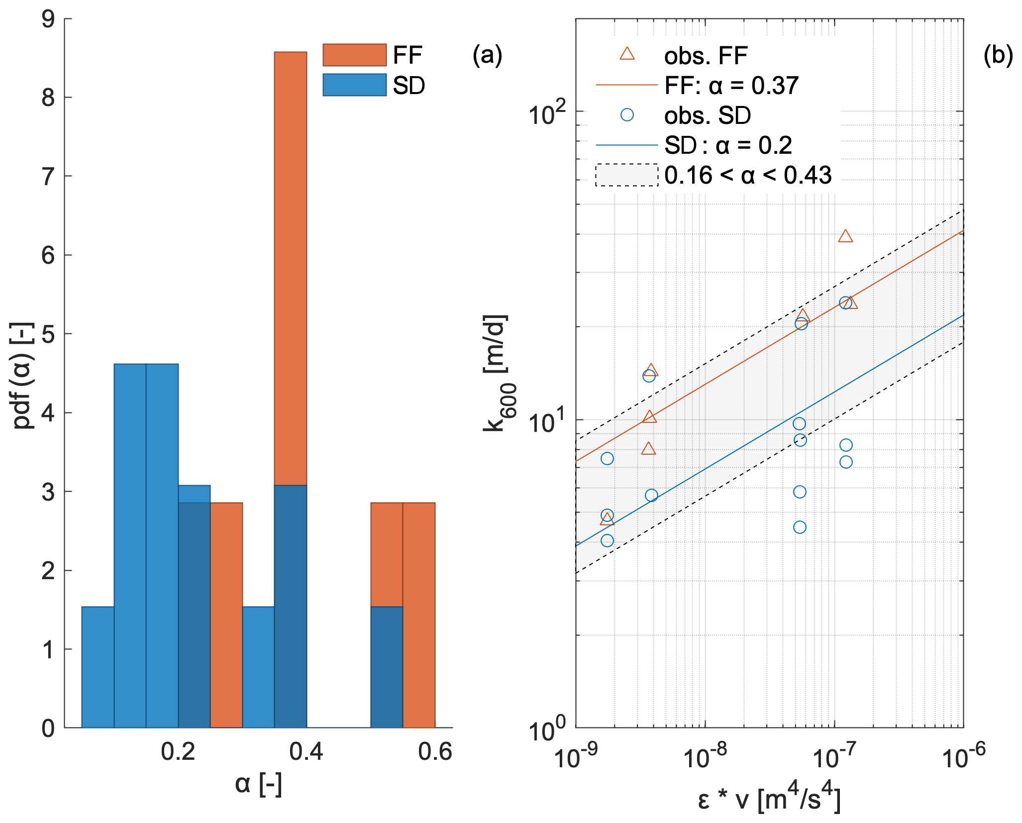
Figure 3Panel (a) contains the probability density function (PDF) of the α coefficient calibrated for each saturation curve for both the flexible foil and standard chamber. Panel (b) shows Eq. (5) obtained for both the standard and the flexible foil chamber in a log–log plot; the coefficient α was calibrated based on the two data sets using the least-square method.
3.5 Comparison with existing scaling laws
Both flexible foil and standard chambers in anchored mode showed increasing values of k600 when the energy dissipation rate of the flow increased. However, the increase in gas exchange velocities over a unit of energy dissipation rate was markedly different for the two chambers under anchored mode. The analysis of data gathered in a drifting mode did not show the expected pattern of k600 with ε for the standard chamber. Instead, the flexible foil chamber produced consistent results between anchored and drifting deployments, with a monotonous increase in k600 with ε (Fig. 3b).
When we compared the relationship of k600 with ε of our measured data with the scaling relationship SL1, we observed both chambers giving reasonable results (see Fig. 3b). In Fig. 3a we show the overall probability density function (PDF) of the coefficient α in Eq. (5) calibrated for each single saturation curve for flexible foil and standard chambers across all the runs. Calibrating α on the single saturation curve allowed the variability of α throughout the experiment to be determined for both the chambers. In Fig. 3b we show the scaling equations (orange and blue) we got through the calibration of α based on all the measurements. The result further enforces the robustness of the data from our steady chambers, since both the curves fall inside the literature range (represented as a light grey shaded area). According to Esters et al. (2017), the coefficient α follows the strong depth dependency in ε. While Esters et al. (2017) refer to standing waters, this can also be expected to be true in running waters where ε varies with depth as a result of bottom friction (Sukhodolov et al., 1998). Therefore, an in-depth comparison between our results and previous studies proves difficult because of the different measuring depths across the studies.
Our results showed a significant linear correlation between log(εemp) and log(k600) (R2=0.23, n=20, p=0.033), in line with Ulseth et al. (2019). By performing a least-square regression on the data gathered using the chambers we noted that only the flexible foil chamber identified a statistically significant positive relationship between log(εemp) and log(k600) (standard: R2=0.16, n=13, p=0.19; flexible foil: R2=0.81, n=7, p=0.006). However, the corresponding coefficients lay outside the 95 % CI range (from 0.31 to 0.41) given by Ulseth et al. (2019). We propose that the reason that explains the observed difference between the scaling exponents derived in this paper and the values available from Ulseth et al. (2019) is represented by the specific set-up of this study (i.e. an artificial flume monitored by means of floating chambers), which differs significantly from that used by Ulseth et al. (2019) (i.e. gas tracer injections in natural streams).
It is worth emphasizing that both scaling relationships explored here are based on the idea that the air–water gas exchange is driven by turbulence; however, SL1 hangs on a theoretical estimate from turbulent velocity fluctuations (ε), whereas SL2 holds on estimates (εemp) from geomorphic variables (see Sect. 2.5). Estimating turbulence from geomorphic properties is a common approach in the literature (Ulseth et al., 2019, and references therein). Here, we obtained good correlations between estimates of ε and εemp for each set-up, with an increasing ratio between ε and εemp (from 3.6 to 16) in more energetic set-ups. This suggests the εemp values are more reliable estimates in low-energy streams.
3.6 Analysis of the uncertainty
The uncertainty in the estimate of gas-exchange velocities and equilibrium concentration via the exponential model (method 2) was analysed using a GLUE technique (see Sect. 2.6). In most cases, the posterior bi-variate distribution was found to be hump-shaped, peaking around the pair of values that provided the best fitting (i.e. maximum NSE, identified by the orange star in Fig. 4). However, this was not always the case. In particular, for runs that were too short to reach full saturation, we often found heterogeneous pairs of and k600 values that performed equally well. The GLUE procedure allowed us to derive a range of likely parameters associated with each saturation curve, providing a tool to characterize the robustness of the best fit obtained during the model calibration phase. It is worth noting that the GLUE procedure could also be used to analyse the uncertainty in the estimate of k600 obtained from the application of method 1 to the data gathered via the drifting chambers. However, method 1 is intrinsically associated with high uncertainties because each experiment performed in the drifting mode consisted of very few observations (see Sect.3.3). Consequently, model performances were lower than those obtained with a steady chamber, and the uncertainty was high. In particular, the standard deviation of the posterior PDF of k600 resulting from method 1 was typically 1 to 2 orders of magnitude higher than the posterior standard deviation obtained using method 2. For method 1, most of the uncertainty is induced by the lack of information on during the drifting runs, which represents a direct consequence of the limited number of available CO2 observations. The above result highlights the value of long-lasting chamber runs that contain several consecutive CO2 measurements in reducing the uncertainty of the estimate of k600.
To assess the uncertainty associated with the average values of k600 derived from method 2 for each set-up (with the flexible foil and standard chambers), we calculated the average among the posterior PDFs associated with each run for a certain set-up and chamber. Practically, we considered all the experiments made with a given chamber for each set-up and we took all the pairs of parameters (k600 and ) that were able to reproduce (with a pre-defined minimum degree of performance) the different saturation curves available. Thus, we ended up with a bi-variate probability density function for and k600 associated with a given threshold performance (in this case NSEt=0.98). The analysis of the uncertainty associated with the estimate of k600 is shown in Fig. 5, where the overall posterior PDFs of k600 obtained across all the set-ups are presented for the flexible foil (orange) and the standard (blue) chamber. The mean k600 from the best-fitting procedure (Table 3) was very close to the corresponding posterior mean for all the chambers and settings. This result reinforces the robustness of the results shown in Table 3. Overall, the uncertainty in the estimate of k600 was moderate to high (standard deviations of the posterior PDFs were in the range 1.6 to 8.2 m d−1). In particular, the standard chamber showed a mean posterior standard deviation that was 20 % higher than that of the flexible foil chamber (see also Table 3). In set-up 3 and 4 the posterior PDFs obtained with the standard chamber were bi-modal. Moreover, they partially overlapped with the posterior PDFs obtained with the flexible foil chamber in correspondence with their posterior mean. As the posterior PDFs represent the likelihood of different parameter values in the light of the available observations, this overlapping indicates that the values of k600 that allowed a good match of the data gathered with the flexible foil chamber (i.e. the posterior modes in Fig. 5e and g) also provided a reasonably good fit to the saturation curves obtained through the standard chamber in the same configurations, at least for some runs. This result is yet another indication that the estimates of k600 provided by the flexible foil chamber were most likely more robust than the estimates obtained using a standard chamber.
We also analysed the error associated with the estimate of k600 shown in Table 3, where the mean values of k600 resulting from all the runs of each set-up are shown. The analysis consisted of calculating the maximum performance achievable for a given set-up using a single value of k600 for all the runs performed in that set-up. When a single value of k600 is calibrated against all the runs of every set-up, for some runs of the standard chamber the performance of the exponential model was lower than that obtained using the flexible foil chamber. For instance, in set-up 4 we had a minimum NSE across all the runs of 0.95 for the standard chamber and a minimum NSE of 0.98 for the flexible foil chamber. In other words, with the standard chamber we could not find a unique set of model parameters that was able to properly fit all the individual runs performed in some set-ups. This is a manifestation of the limited degree of overlapping among the posterior PDFs associated with each single run of a given set-up when the standard chamber was used.
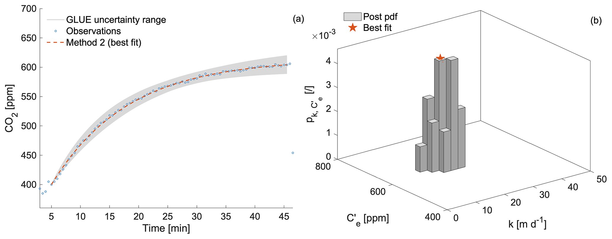
Figure 4Panel (a) contains the observations of CO2 with the flexible foil chamber – steady mode – for set-up 4. The curve in orange is the result of the fitting procedure with method 2. Panel (b) contains the bi-variate posterior PDF of k and ; the orange dot indicates the optimal parameters resulting from the fitting procedure with method 2.
The GLUE analysis also enabled the identification of the relative contributions to the total uncertainty in our k600 estimate associated with (i) the uncertainty of model fitting during a single run and (ii) the uncertainty induced by heterogeneity among replicate runs. This was done by comparing the posterior PDF associated with a single run and that obtained by averaging the results of all the runs performed under the same conditions. The GLUE analysis evidenced a non-negligible uncertainty associated with the fitting of the exponential model to the data derived from a single run. As illustrated in Fig. 5a and c, the estimate of the gas exchange velocity from a single experiment had an intrinsic uncertainty, which was about 25 % of the best-fit value of k600. Interestingly, the uncertainty in k600 estimates associated with single runs increased slightly with increasing ε in all the available cases. Furthermore, we observed that the heterogeneity among replicate experiments generated an additional contribution to the uncertainty for all the set-ups in which replicate experiments were performed. This uncertainty accounted for the variability of the physical, environmental and hydrodynamic conditions experienced by the chamber during runs that were performed at different times and dates under the same conditions (chamber type and set-up). The contribution to the total uncertainty of k600 induced by the heterogeneity of replicate measurements markedly increased (i.e. more than linearly) with ε. Consequently, above a certain threshold of ε the uncertainty of k600 was dominated by the heterogeneity of the saturation curves associated with replicate measurements. This emphasizes the value of replicated experiments performed under the same conditions in quantifying the uncertainty of k600 estimations within systems characterized by high ε.

Figure 5Overall posterior marginal PDF of k600 for each different set-up (1, 2, 3, 4) and for both flexible foil (orange: a, c, e, g) and standard (blue: b, d, f, h) chambers. The PDFs were obtained using a threshold performance (NSEt) of 0.98. The green stars indicate the best fit from Table 3, while the diamonds represent the posterior averages.
In this paper we analysed the results of a flume experiment aimed at the quantification of k600 via the application of the floating chamber methodology. During the experiment, two chamber designs (standard vs. flexible foil) and two deployment modes (anchored vs. drifting) were compared, and the uncertainty in the estimate of the gas transfer velocity was analysed using the GLUE procedure. The main conclusions of the work can be summarized as follows:
-
Overall, our estimates of gas exchange velocities and water equilibrium concentrations were in line with previous results (Moog and Jirka, 1999; Zappa et al., 2007; Tokoro et al., 2008; Vachon et al., 2010; Schelker et al., 2016; Ulseth et al., 2019), with a general increase in the gas exchange velocity for larger turbulent kinetic energy dissipation rates.
-
Differently from the standard chamber, in most set-ups the flexible foil chamber exhibited coherent results between runs performed under the same conditions with different deployment modes (anchored or drifting). Thus we propose that the flexible foil chamber can ensure a greater flexibility of use (drifting or anchored deployments) across a wide range of field conditions.
-
The flexible foil chamber gave consistent k600 responses to changes in the slope and/or discharge in all the set-ups. Moreover, the ADV measurements carried out below the chambers during the runs indicated that the estimate of k600 was biased by only + 6 % owing to the impact of the flexible foil chamber on the underlying flow field. Conversely, the bias increased to + 18 % when the standard chamber was used. The limited turbulence induced by our flexible foil chamber and its ability to replicate previously observed relationships between k600 and slope, discharge and kinetic energy makes it a promising tool for future stream CO2 studies.
-
In our experiment, uncertainty in the estimate of gas exchange velocity was moderate to high, with standard deviations of k600 between 1.6 and 8.2 m d−1 for the anchored mode. Drifting deployments, instead, were typically characterized by a larger uncertainty, with a huge increase in the uncertainty of k600 estimates mainly due to the lack of information on during the drifting runs. While drifting deployments allow useful estimates of spatially integrated k600 within whole river segments, our results highlighted the value of steady runs for limiting the uncertainty of water equilibrium concentrations and gas exchange velocities in streams.
-
The comparison of the uncertainty in k600 estimates obtained using different chamber types evidenced that a smaller uncertainty is associated with the flexible foil chamber (− 20 % with respect to the standard chamber). Likewise, when a single k600 is associated with all the runs of a given set-up, the exponential model had a poorer fitting to the data obtained with the standard chamber as compared to the flexible foil chamber, because of the enhanced heterogeneity of the different runs performed with the standard chamber.
-
Our study highlighted the importance of quantifying different sources of errors in the estimate of gas exchange velocities derived via the chamber methodology. While the uncertainty in k600 estimates was dependent on the chamber design and the deployment technique, in general uncertainty was higher in systems with a high turbulent kinetic energy dissipation rate, where the heterogeneity among replicate experiments dominates. Thus, we propose that performing different replicate experiments under the same conditions should become a standard practice in the quantification of the magnitude (and the uncertainty) of gas exchange velocities, particularly in high-energy hydrologic systems.
In conclusion, this study indicated that the flexible foil chamber used in an anchored deployment mode is able to enhance the reliability and decrease the uncertainty of CO2 measurements in low-order streams. Furthermore, the analyses shown in the paper allowed us to identify an objective procedure to properly handle model parameter uncertainty in CO2 outgassing studies based on the chamber methodology. These findings can be easily generalized to other soluble gases transported by non-bubbly flows, with potentially important implications for the estimate of gas exchange processes in running water.
In order to compute ε, flow velocities were measured in four directions using an acoustic Doppler velocity meter (Vectrino+, down-looking probe, Nortek, Rud, Norway). For each experiment, we took 24 measurements along 6 transects crossing the flume profile, with 4 measurements per transect. The probe was sampled at 200 Hz, with a preset velocity range of 0.1 to 0.3 or 0.3 to 1 m, a sampling volume height of 7 mm and a transmit length of 1.8 mm. The probe was mounted to a custom-made frame and tilted (heading = 0∘, roll = 45∘, pitch = 57∘) to allow measurements at 5–6 cm below the water surface. To increase the scatter of the acoustic pulse emitted from the probe, we enhanced the turbidity of the inflowing water by adding a solution of wheat flour and water (120 g L−1) at constant flow rates (50–80 mL min−1) using a peristaltic pump (Schlauchpumpe MV-GE, Ismatec Cole-Parmer GmbH, Wertheim, Germany). This set-up allowed nearly spike-free recordings with signal-to-noise ratios (SNRs) of 21.5 ± 2.1 (mean ± SD) and correlations of 92.2 ± 5.2 %. We rejected time series with SNRs < 15 and correlations < 70. We identified the few spikes remaining in accepted time series using the three-dimensional phase space method developed by Goring and Nikora (2002) with modifications by Mori et al. (2007). We interpolated spikes using cubic polynomials. For despiking and interpolation, we used code by Mori (2020). We rotated the despiked velocities into a vertically oriented earth coordinate system with an along-flow (u), cross-flow (v) and two duplicate up–down (w1, w2) components following standard transformations provided by Nortek (2020). We estimated ε using the inertial dissipation method following Zappa et al. (2003) with modifications by Bluteau et al. (2011). Accordingly, the kinetic energy of isotropic turbulence is dissipated by breaking larger to smaller eddies within the inertial subrange of wave numbers. ε can be derived from the wave number spectrum (S) of the fluctuating velocities of component as follows:
where c=1.5 is the empirical Kolmogorov universal constant, for the component in the direction of mean advection, in the other directions perpendicular (i=2) or vertical (i=3) to the direction of mean advection (Pope, 2000), is the wave number, f is the frequency, and uadv is the mean advection velocity. We derived the wave number spectra of fluctuating velocities from the frequency spectra, assuming Taylor’s hypothesis of frozen turbulence, i.e. turbulent motions, quantified by the root mean square of fluctuating velocities (si), are small relative to uadv. We calculated uadv by rotating the velocities such that following Foken (2008). In our experiment was always <0.04, giving strong support to the frozen turbulence hypothesis (Kitaigorodskii and Lumley, 1983). We generated the frequency spectra by means of Welch’s method using eight segments with 50 % overlap and tapered with a Hamming window. We corrected the measured frequency spectra for pulse averaging by dividing them by [a1(f)+a2(f)], where
and f_0=200 Hz is the nominal sampling frequency (Henjes et al., 1999). To find the inertial subrange within which ε is calculated, we used an approach following recommendations by Bluteau et al. (2011). Specifically, we fitted Eq. (5) to the measured spectra within wave number intervals of different widths and locations along the wave number axis. To define these “candidate” intervals, we evaluated all possible combinations of lower and upper interval bounds. We set the minimum lower bound to and the maximum upper bound to , where D is the distance of the ADV sampling volume from the water surface (m) and L is the length scale (m) of the ADV sampling volume (cf. Zappa et al., 2003). We also required S to drop by at least 1 order of magnitude within the bounds (Bluteau et al., 2011). For each “candidate” interval, we modelled the wave number spectrum using maximum likelihood estimation following Bluteau et al. (2011), assuming that the ratio of observed () and modelled (S) spectral estimates follows a distribution (), where df represents the degrees of freedom of the system. Using the probability density function of the distribution,
we computed the log likelihood for spectral observations
in order to find the most likely estimate for ε for the specific wave number interval. We determined the minimum 95 % confidence interval of ε as , where var(ε) is the variance of ε calculated based on the curvature of the maximum log likelihood:
To evaluate the goodness of fit for each “candidate” interval, we computed the maximum absolute deviation (MAD):
following Ruddick et al. (2000). The interval that yielded the lowest MAD was used to determine the final ε estimate. As an additional measure of the goodness of fit, we calculated the coefficient of determination:
We rejected all ε estimates with MAD > 2 or R2<0. For comparison with flume-integrated k600 values, we averaged log-normally distributed ε following Baker and Gibson (1987). In averaging, we included all estimates of the vertical component for which the 95 % confidence intervals of these estimates overlapped with the corresponding estimates of the other directions (εu, εv) overlapped; i.e. the assumption of isotropic turbulence was fulfilled. Overall, 82 % of all ADV measurements passed all our quality requirements and were used for ε estimation. Code to calculate epsilon from the ADV data is provided under the GPL-3.0 licence at https://github.com/MarcusKlaus/CalculateEpsilon (last access: 11 November 2020).
In order to compare the results of k with other gas exchange velocities at 20 ∘C, the observed values of k were converted to a standardized gas exchange rate k600 as follows:
where the subscript 600 indicates the Schmidt number of CO2 at 20 ∘C in freshwater. The exponent n in Eq. (B1) is usually between and 1; is more appropriate for rough surfaces, for calm waters (Rawitch et al., 2019). Therefore, is a proper value for our analyses. The Schmidt number (Sc) is a dimensionless number expressing the ratio between the kinematic viscosity of water to the diffusivity of gas. Sc of CO2 () can be estimated from water temperature (Tw) via the following expression (Raymond et al., 2012):
Standardization to k600 requires the knowledge of the water temperature, which was unknown during the experiment. In order to overcome this issue, we decided to use a unique time–temperature relationship derived from the interpolation of the few available data even though we are conscious of the possible biases because of the change in daily temperature cycles during the experiment. Given the observed maximum diurnal water temperature excursion (10–15 ∘C), the possible influence of errors in temperature on the k600 estimate is limited (± 8 %).
Figure C1 contains three photos from different perspectives of the flexible foil chamber. An overview of flexible foil chamber (Fig. C1a) shows the floating system designed via three 0.5 L water bottles. In order to have a real-time control on the measurement a top casing containing the USB connection to the sensor was developed (Fig. C1a). The rigid cup of the chamber was sustained above the water surface by the floating system that was fixed on the external cup margin (Fig. C1b). The flexible sealing via polyethylene foil (Plastic sheet UV4, Foliarex, Poznań, Poland) and adhesive tape (Extra Power Universal, Tesa, Hamburg, Germany) was extended all around the lower internal profile of the chamber cup (Fig. C1b). The sealing guaranteed a complete isolation of the air inside the chamber from the external atmosphere. An open protection of the CO2 sensor was developed to prevent contact with water droplets (Fig. C1c).
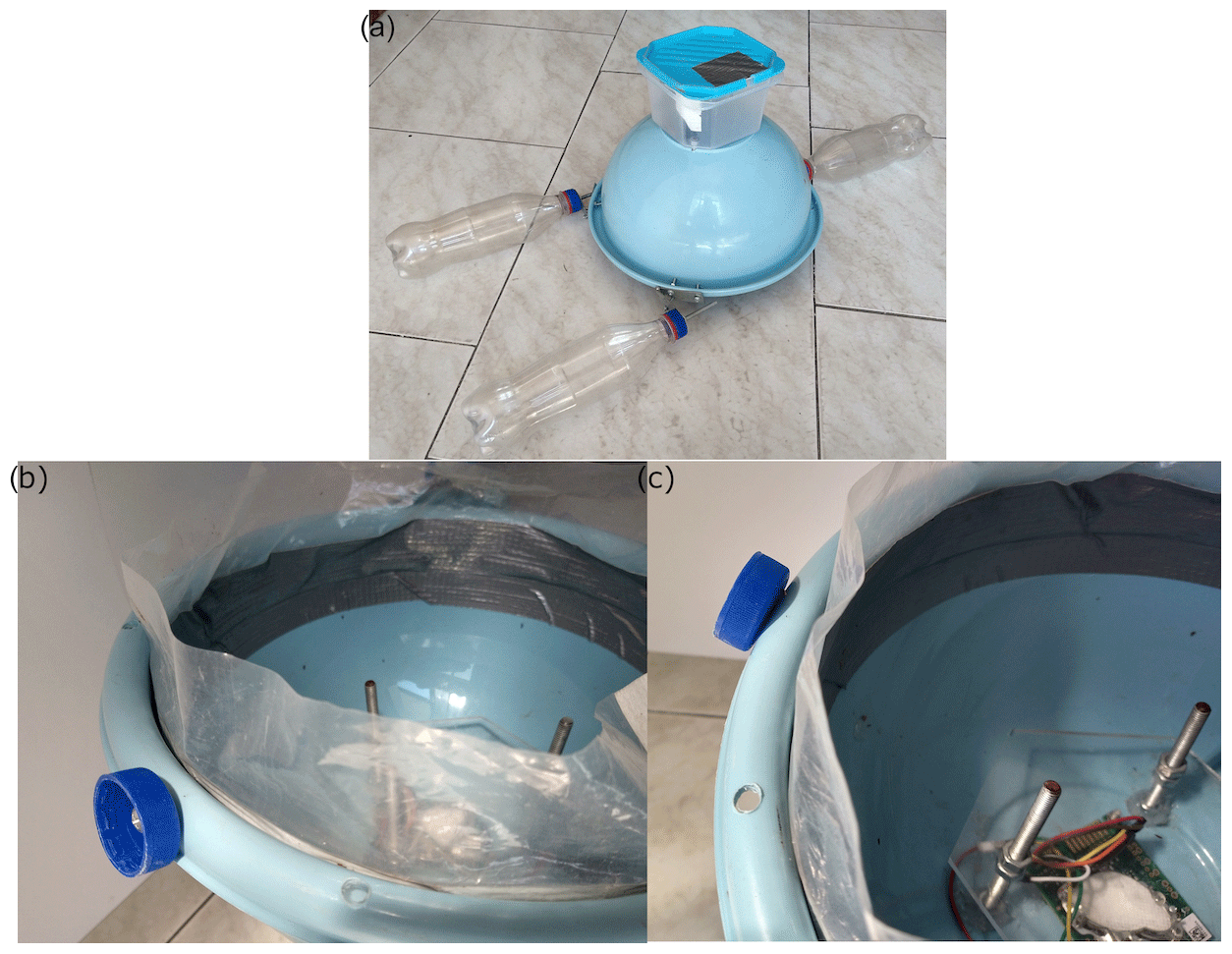
Figure C1Overview of the flexible foil chamber (a). Close-up of the support of the floating system (b). Protection of the sensor from the water droplets (c).
Experimental data collected for this study and codes used for the analysis are available at Vingiani et al. (2021).
All authors contributed to designing and performing the experiment in Lunz. ND designed and built the flexible foil chamber. FV analysed the chamber results and wrote a first draft of the paper. GB identified the methods for the analysis and, together with MK and JS, provided insight into data interpretation. MK performed the ADV measurements and analysed the ADV data. All authors contributed to finalizing and editing the paper.
The authors declare that they have no conflict of interest.
We thank Michael Scharner and Paul Schweigerlehner for field assistance, Gertraud Stenizcka for logistical assistance and Johann Waringer for providing the ADV system.
This research has been supported by the European Community's Horizon 2020 Excellent Science Programme (grant no. H2020-EU.1.1.-770999) and the European Commission EU H2020-INFRAIA-project AQUACOSM (grant no. 731065).
This paper was edited by Tyler Cyronak and reviewed by two anonymous referees.
Alin, S. R., de Fátima F. L. Rasera, M., Salimon, C. I., Richey, J. E., Holtgrieve, G. W., Krusche, A. V., and Snidvongs, A.: Physical controls on carbon dioxide transfer velocity and flux in low-gradient river systems and implications for regional carbon budgets, J. Geophys. Res.-Biogeo., 116, G1, https://doi.org/10.1029/2010JG001398, 2011. a
Baker, M. A. and Gibson, C. H.: Sampling Turbulence in the Stratified Ocean: Statistical Consequences of Strong Intermittency, J. Phys. Oceanogr., 17, 1817–1836, https://doi.org/10.1175/1520-0485(1987)017<1817:STITSO>2.0.CO;2, 1987. a
Bastviken, D., Cole, J., Pace, M., and Tranvik, L.: Methane emissions from lakes: Dependence of lake characteristics, two regional assessments, and a global estimate, Global Biogeochem. Cy., 18, 4, https://doi.org/10.1029/2004GB002238, 2004. a
Bastviken, D., Sundgren, I., Natchimuthu, S., Reyier, H., and Gålfalk, M.: Technical Note: Cost-efficient approaches to measure carbon dioxide (CO2) fluxes and concentrations in terrestrial and aquatic environments using mini loggers, Biogeosciences, 12, 3849–3859, https://doi.org/10.5194/bg-12-3849-2015, 2015. a, b, c, d, e, f
Battin, T. J., Luyssaert, S., Kaplan, L. A., Aufdenkampe, A. K., Richter, A., and Tranvik, L. J.: The boundless carbon cycle, Nat. Geosci., 2, 598–600, https://doi.org/10.1038/ngeo618, 2009. a
Beaulieu, J. J., Shuster, W. D., and Rebholz, J. A.: Controls on gas transfer velocities in a large river, J. Geophys. Res.-Biogeo., 117, G2, https://doi.org/10.1029/2011JG001794, 2012. a
Beven, K. and Binley, A.: The future of distributed models: Model calibration and uncertainty prediction, Hydrol. Process., 6, 279–298, https://doi.org/10.1002/hyp.3360060305, 1992. a
Bluteau, C. E., Jones, N. L., and Ivey, G. N.: Estimating turbulent kinetic energy dissipation using the inertial subrange method in environmental flows, Limnol. Oceanogr.-Meth., 9, 302–321, https://doi.org/10.4319/lom.2011.9.302, 2011. a, b, c, d
Boodoo, K. S., Schelker, J., Trauth, N., Battin, T. J., and Schmidt, C.: Sources and variability of CO2 in a prealpine stream gravel bar, Hydrol. Process., 33, 2279–2299, https://doi.org/10.1002/hyp.13450, 2019. a
Department of Scientific and Industrial Research: Effects of Polluting Discharges on the Thames Estuary, The Reports of the Thames Survey Committee and the Water Pollution Research Laboratory, Water Pollution Research Technical Paper, No. 11, vol. 252s, Her majesty's Stationery Office, London, , 1964. a
Esters, L., Landwehr, S., Sutherland, G., Bell, T. G., Christensen, K. H., Saltzman, E. S., Miller, S. D., and Ward, B.: Parameterizing air-sea gas transfer velocity with dissipation, J. Geophys. Res.-Oceans, 122, 3041–3056, https://doi.org/10.1002/2016JC012088, 2017. a, b
Foken, T.: Micrometeorology, Springer-Verlag Berlin Heidelberg, 2008. a
Gålfalk, M., Bastviken, D., Fredriksson, S., and Arneborg, L.: Determination of the piston velocity for water-air interfaces using flux chambers, acoustic Doppler velocimetry, and IR imaging of the water surface, J. Geophys. Res.-Biogeo., 118, 770–782, https://doi.org/10.1002/jgrg.20064, 2013. a
Goring, D. G. and Nikora, V. I.: De-spiking Acoustic Doppler Velocimeter data, J. Hydraul. Eng., 128, 117–126, https://doi.org/10.1061/(ASCE)0733-9429(2002)128:1(117), 2002. a
Hall, R. O. and Ulseth, A. J.: Gas exchange in streams and rivers, WIRES Water, 7, e1391, https://doi.org/10.1002/wat2.1391, 2020. a, b, c, d
Henjes, K., Taylor, P. K., and Yelland, M. J.: Effect of Pulse Averaging on Sonic Anemometer Spectra, J. Atmos. Ocean. Tech., 16, 181–184, https://doi.org/10.1175/1520-0426(1999)016<0181:EOPAOS>2.0.CO;2, 1999. a
Horgby, Å. s., Segatto, P., Bertuzzo, E., Lauerwald, R., Lehner, B., Ulseth, A., Vennemann, T., and Battin, T.: Unexpected large evasion fluxes of carbon dioxide from turbulent streams draining the world’s mountains, Nat. Commun., 10, 4888, https://doi.org/10.1038/s41467-019-12905-z, 2019. a
Hotchkiss, E. R., Hall Jr, R. O., Sponseller, R. A., Butman, D., Klaminder, J., Laudon, H., Rosvall, M., and Karlsson, J.: Sources of and processes controlling CO2 emissions change with the size of streams and rivers, Nat. Geosci., 8, 696–699, https://doi.org/10.1038/ngeo2507, 2015. a
Jeffrey, L. C., Maher, D. T., Santos, I. R., Call, M., Reading, M. J., Holloway, C., and Tait, D. R.: The spatial and temporal drivers of pCO2, pCH4 and gas transfer velocity within a subtropical estuary, Estuar. Coast Shelf, 208, 83–95, https://doi.org/10.1016/j.ecss.2018.04.022, 2018. a, b
Kitaigorodskii, S. A. and Lumley, J. L.: Wave-Turbulence interactions in the Upper Ocean. Part I: The Energy Balance of the Interacting Fields of Surface Wind Waves and Wind-Induced Three-Dimensional Turbulence, J. Phys. Oceanogr., 13, 1977–1987, https://doi.org/10.1175/1520-0485(1983)013<1977:WTIITU>2.0.CO;2, 1983. a
Lorke, A., Bodmer, P., Noss, C., Alshboul, Z., Koschorreck, M., Somlai-Haase, C., Bastviken, D., Flury, S., McGinnis, D. F., Maeck, A., Müller, D., and Premke, K.: Technical note: drifting versus anchored flux chambers for measuring greenhouse gas emissions from running waters, Biogeosciences, 12, 7013–7024, https://doi.org/10.5194/bg-12-7013-2015, 2015. a, b, c, d, e, f
Lorke, A., Bodmer, P., Koca, K., and Noss, C.: Hydrodynamic control of gas-exchange velocity in small streams, https://doi.org/10.31223/osf.io/8u6vc, 2019. a
Mannich, M., Fernandes, C., and Bleninger, T.: Uncertainty analysis of gas flux measurements at air–water interface using floating chambers, Ecohydrol. Hydrobiol., 19, 475–486, https://doi.org/10.1016/j.ecohyd.2017.09.002, 2019. a
Marx, A., Dusek, J., Jankovec, J., Sanda, M., Vogel, T., van Geldern, R., Hartmann, J., and Barth, J. A. C.: A review of CO2 and associated carbon dynamics in headwater streams: A global perspective, Rev. Geophys., 55, 560–585, https://doi.org/10.1002/2016RG000547, 2017. a
Maurice, L., Rawlins, B. G., Farr, G., Bell, R., and Gooddy, D. C.: The Influence of Flow and Bed Slope on Gas Transfer in Steep Streams and Their Implications for Evasion of CO2, J. Geophys. Res.-Biogeo., 122, 2862–2875, https://doi.org/10.1002/2017JG004045, 2017. a
Moog, D. B. and Jirka, G. H.: Air-Water Gas Transfer in Uniform Channel Flow, J. Hydraul. Eng., 125, 3–10, https://doi.org/10.1061/(ASCE)0733-9429(1999)125:1(3), 1999. a, b
Moore, R.: Introduction to salt dilution gauging for streamflow measurement part 2: Constant-rate injection, available at: https://pdfs.semanticscholar.org/4210/42e4d7a842b6be48ec746b1453a82fb3ed5e.pdf, (last access: 25 June 2020), 2004. a
Moore, R.: Introduction to Salt Dilution Gauging for Streamflow Measurement Part III: Slug Injection Using Salt in Solution, available at: https://www.uvm.edu/bwrl/lab_docs/protocols/2005_Moore_Slug_salt_dilution_gauging_volumetric_method_Streamline.pdf, (last access: 25 June 2020), 2005. a
Mori, N.: Despiking, available at: https://www.mathworks.com/matlabcentral/fileexchange/15361-despiking, MATLAB Central File Exchange, retrieved: 1 November 2020. a
Mori, N., Suzuki, T., and Kakuno, S.: Noise of Acoustic Doppler Velocimeter Data in Bubbly Flows, J. Eng. Mech., 133, 122–125, https://doi.org/10.1061/(ASCE)0733-9399(2007)133:1(122), 2007. a
Natchimuthu, S., Wallin, M. B., Klemedtsson, L., and Bastviken, D.: Spatio-temporal patterns of stream methane and carbon dioxide emissions in a hemiboreal catchment in Southwest Sweden, Sci. Rep.-UK, 7, 39729, https://doi.org/10.1038/srep39729, 2017. a
Nortek: How is a Coordinate transformation done?, available at: https://support.nortekgroup.com/hc/en-us/articles/360029820971-How-is-a-Coordinate-transformation-done- (last access: 29 March 2020), 2020. a
Peter, H., Singer, G. A., Preiler, C., Chifflard, P., Steniczka, G., and Battin, T. J.: Scales and drivers of temporal pCO2 dynamics in an Alpine stream, J. Geophys. Res.-Biogeo., 119, 1078–1091, https://doi.org/10.1002/2013JG002552, 2014. a, b, c, d
Ploum, S. W., Leach, J. A., Kuglerová, L., and Laudon, H.: Thermal detection of discrete riparian inflow points (DRIPs) during contrasting hydrological events, Hydrol. Process., 32, 3049–3050, https://doi.org/10.1002/hyp.13184, 2018. a
Podgrajsek, E., Sahlée, E., Bastviken, D., Holst, J., Lindroth, A., Tranvik, L., and Rutgersson, A.: Comparison of floating chamber and eddy covariance measurements of lake greenhouse gas fluxes, Biogeosciences, 11, 4225–4233, https://doi.org/10.5194/bg-11-4225-2014, 2014. a
Pope, S. B.: Turbulent Flows, Cambridge University Press, United States of America by Cambridge University Press, New York, 2000. a
Rawitch, M. J., Macpherson, G. L., and Brookfield, A. E.: Exploring methods of measuring CO2 degassing in headwater streams, Sust. Water Resour. Manag., 5, 1765–1779, https://doi.org/10.1007/s40899-019-00332-3, 2019. a, b, c, d
Raymond, P. A., Zappa, C. J., Butman, D., Bott, T. L., Potter, J., Mulholland, P., Laursen, A. E., McDowell, W. H., and Newbold, D.: Scaling the gas transfer velocity and hydraulic geometry in streams and small rivers, Limnol. Oceanogr., 2, 41–53, https://doi.org/10.1215/21573689-1597669, 2012. a, b, c, d, e
Raymond, P. A., Hartmann, J., Lauerwald, R., Sobek, S., McDonald, C., Hoover, M., Butman, D., Striegl, R., Mayorga, E., Humborg, C., Kortelainen, P., Dürr, H., Meybeck, M., Ciais, P., and Guth, P.: Global carbon dioxide emissions from inland waters, Nature, 503, 355–359, https://doi.org/10.1038/nature12760, 2013. a, b, c
Rosentreter, J. A., Maher, D. T., Ho, D. T., Call, M., Barr, J. G., and Eyre, B. D.: Spatial and temporal variability of CO2 and CH4 gas transfer velocities and quantification of the CH4 microbubble flux in mangrove dominated estuaries, Limnol. Oceanogr., 62, 561–578, https://doi.org/10.1002/lno.10444, 2017. a
Ruddick, B., Anis, A., and Thompson, K.: Maximum Likelihood Spectral Fitting: The Batchelor Spectrum, J. Atmos. Ocean. Tech., 17, 1541–1555, https://doi.org/10.1175/1520-0426(2000)017<1541:MLSFTB>2.0.CO;2, 2000. a
Sand-Jensen, K. and Staehr, P. A.: CO2 dynamics along Danish lowland streams: water–air gradients, piston velocities and evasion rates, Biogeochemistry, 111, 615–628, https://doi.org/10.1007/s10533-011-9696-6, 2012. a, b, c
Sander, R.: Compilation of Henry's law constants (version 4.0) for water as solvent, Atmos. Chem. Phys., 15, 4399–4981, https://doi.org/10.5194/acp-15-4399-2015, 2015. a
Sawakuchi, H. O., Neu, V., Ward, N. D., Barros, M. d. L. C., Valerio, A. M., Gagne-Maynard, W., Cunha, A. C., Less, D. F. S., Diniz, J. E. M., Brito, D. C., Krusche, A. V., and Richey, J. E.: Carbon Dioxide Emissions along the Lower Amazon River, Front. Mar. Sci., 4, 76, https://doi.org/10.3389/fmars.2017.00076, 2017. a
Schelker, J., Singer, G. A., Ulseth, A. J., Hengsberger, S., and Battin, T. J.: CO2 evasion from a steep, high gradient stream network: importance of seasonal and diurnal variation in aquatic pCO2 and gas transfer: CO2 evasion from a steep, high gradient stream network, Limnol. Oceanogr., 61, 1826–1838, https://doi.org/10.1002/lno.10339, 2016. a, b, c, d
Sukhodolov, A., Thiele, M., and Bungartz, H.: Turbulence structure in a river reach with sand bed, Water Resour Res, 34, 1317–1334, https://doi.org/10.1029/98WR00269, 1998. a
Tokoro, T., Kayanne, H., Watanabe, A., Nadaoka, K., Tamura, H., Nozaki, K., Kato, K., and Negishi, A.: High gas-transfer velocity in coastal regions with high energy-dissipation rates, J. Geophys. Res.-Oceans, 113, https://doi.org/10.1029/2007JC004528, 2008. a, b
Ulseth, A., Hall, R., Canadell, M., Madinger, H., Niayifar, A., and Battin, T.: Distinct air–water gas exchange regimes in low- and high-energy streams, Nat. Geosci., 12, 1–5, https://doi.org/10.1038/s41561-019-0324-8, 2019. a, b, c, d, e, f, g, h, i
Vachon, D., Prairie, Y. T., and Cole, J. J.: The relationship between near-surface turbulence and gas transfer velocity in freshwater systems and its implications for floating chamber measurements of gas exchange, Limnol. Oceanogr., 55, 1723–1732, https://doi.org/10.4319/lo.2010.55.4.1723, 2010. a, b, c
Vingiani, F., Durighetto, N., Klaus, M., Schelker, J., Labasque, T., and Botter, G.: Evaluating stream CO2 outgassing via drifting and anchored flux chambers in a controlled flume experiment, https://doi.org/10.25430/researchdata.cab.unipd.it.00000425, 2021.
Wanninkhof, R., Asher, W. E., Ho, D. T., Sweeney, C., and McGillis, W. R.: Advances in Quantifying Air-Sea Gas Exchange and Environmental Forcing, Annu. Rev. Mar. Sci., 1, 213–244, https://doi.org/10.1146/annurev.marine.010908.163742, 2009. a
Zappa, C. J., Raymond, P. A., Terray, E. A., and McGillis, W. R.: Variation in surface turbulence and the gas transfer velocity over a tidal cycle in a macro-tidal estuary, Estuaries, 26, 1401–1415, https://doi.org/10.1007/BF02803649, 2003. a, b, c, d
Zappa, C. J., McGillis, W. R., Raymond, P. A., Edson, J. B., Hintsa, E. J., Zemmelink, H. J., Dacey, J. W. H., and Ho, D. T.: Environmental turbulent mixing controls on air-water gas exchange in marine and aquatic systems, Geophys. Res. Lett., 34, https://doi.org/10.1029/2006GL028790, 2007. a, b
- Abstract
- Introduction
- Methods
- Results and discussion
- Conclusions
- Appendix A: Turbulent kinetic energy dissipation estimation from ADV measurements
- Appendix B: Standardization of the gas exchange velocity
- Appendix C: Design of the flexible foil chamber
- Code and data availability
- Author contributions
- Competing interests
- Acknowledgements
- Financial support
- Review statement
- References