the Creative Commons Attribution 4.0 License.
the Creative Commons Attribution 4.0 License.
 | 18 Feb 2021
Role of jellyfish in the plankton ecosystem revealed using a global ocean biogeochemical model
Rebecca M. Wright
Corinne Le Quéré
Erik Buitenhuis
Sophie Pitois
Mark J. Gibbons
Jellyfish are increasingly recognised as important components of the marine ecosystem, yet their specific role is poorly defined compared to that of other zooplankton groups. This paper presents the first global ocean biogeochemical model that includes an explicit representation of jellyfish and uses the model to gain insight into the influence of jellyfish on the plankton community. The Plankton Type Ocean Model (PlankTOM11) model groups organisms into plankton functional types (PFTs). The jellyfish PFT is parameterised here based on our synthesis of observations on jellyfish growth, grazing, respiration and mortality rates as functions of temperature and jellyfish biomass. The distribution of jellyfish is unique compared to that of other PFTs in the model. The jellyfish global biomass of 0.13 PgC is within the observational range and comparable to the biomass of other zooplankton and phytoplankton PFTs. The introduction of jellyfish in the model has a large direct influence on the crustacean macrozooplankton PFT and influences indirectly the rest of the plankton ecosystem through trophic cascades. The zooplankton community in PlankTOM11 is highly sensitive to the jellyfish mortality rate, with jellyfish increasingly dominating the zooplankton community as its mortality diminishes. Overall, the results suggest that jellyfish play an important role in regulating global marine plankton ecosystems across plankton community structure, spatio-temporal dynamics and biomass, which is a role that has been generally neglected so far.
- Article
(7440 KB) - Full-text XML
- BibTeX
- EndNote


Gelatinous zooplankton are increasingly recognised as influential organisms in the marine environment – not just for the disruptions they can cause to coastal economies (fisheries, aquaculture, beach closures, power plants, etc.; Purcell et al., 2007) – but also as important consumers of plankton (Lucas and Dawson, 2014), which is a food source for many marine species (Lamb et al., 2017), and as key components in marine biogeochemical cycles (Crum et al., 2014; Lebrato et al., 2012). The term gelatinous zooplankton can encompass a wide range of organisms across three phyla: Tunicata (salps), Ctenophora (comb jellies) and Cnidaria (true jellyfish). This study focuses on Cnidaria (including Hydrozoa, Cubozoa and Scyphozoa), which contribute 92 % of the total global biomass of gelatinous zooplankton (Lucas et al., 2014). The other gelatinous zooplankton groups, Tunicata and Ctenophora, are excluded from this study, because there are far fewer data available on their biomass and vital rates than for Cnidaria; they only contribute a combined global biomass of 8 % of total gelatinous zooplankton (Lucas et al., 2014). Cnidaria are both independent enough from other gelatinous zooplankton and cohesive enough to be represented as a single plankton functional type (PFT) for global modelling (Le Quéré et al., 2005). For the rest of this paper, pelagic Cnidaria are referred to as jellyfish.
Jellyfish exhibit a radially symmetrical body plan and are characterised by a bell-shaped bodies (medusae). Swimming is achieved by muscular, “pulsing” contractions, and the animals have one opening for both feeding and egestion. Most scyphozoans and cubozoans, as well as many hydrozoans, follow a meroplanktonic life cycle. A sessile (generally) benthic polyp buds off planktonic ephyrae asexually. These, in turn, grow into medusae that reproduce sexually to generate planula larvae, which then settle and transform into polyps. Within this general life cycle, there is a large reproductive and life-cycle variety, including some holoplanktonic species that skip the benthic polyp stage, as well as holobenthic species that skip the pelagic phase, and much plasticity (Boero et al., 2008; Lucas and Dawson, 2014).
Jellyfish are significant consumers of plankton, feeding mostly on zooplankton using tentacles and/or oral arms containing stinging cells called nematocysts (Lucas and Dawson, 2014). The high body size to carbon content ratio of jellyfish creates a large low-maintenance feeding structure, which (because they do not use sight to capture prey) allow them to efficiently clear plankton throughout 24 h (Acuña et al., 2011; Lucas and Dawson, 2014). Jellyfish are connected to lower trophic levels, with the ability to influence the plankton ecosystem structure and thus the larger marine ecosystem through trophic cascades (Pitt et al., 2007, 2009; West et al., 2009). Jellyfish have the ability to rapidly form large high-density aggregations known as blooms that can temporarily dominate local ecosystems (Graham et al., 2001; Hamner and Dawson, 2009). Jellyfish contribute to the biogeochemical cycle through two main routes: from life through feeding processes, including the excretion of faecal pellets, mucus and messy-eating debris, and from death through the sinking of carcasses (Chelsky et al., 2015; Lebrato et al., 2012, 2013a; Pitt et al., 2009). The high biomass achieved during jellyfish blooms and the rapid sinking of excretions from feeding and carcasses from such blooms make them a potentially significant vector for carbon export (Lebrato et al., 2013a, b; Luo et al., 2020).
Anthropogenic impacts from climate change, such as increasing temperature and acidity (Rhein et al., 2013), and fishing, such as the removal of predators and competitors (Doney et al., 2012), impact the plankton including jellyfish (Boero et al., 2016; but see Richardson and Gibbons, 2008). Multiple co-occurring impacts make it difficult to understand the role of jellyfish in the marine ecosystem and how the role may be changed by the co-occurring impacts. The paucity of historical jellyfish biomass data, especially outside of coastal regions and the Northern Hemisphere, has made it difficult to establish jellyfish global spatial distribution, biomass and trends from observations (Brotz et al., 2012; Condon et al., 2012; Gibbons and Richardson, 2013; Lucas et al., 2014; Pitt et al., 2018).
Table 1Size range and descriptions of PFT groups used in PlankTOM11. Adapted from Le Quéré et al. (2016).
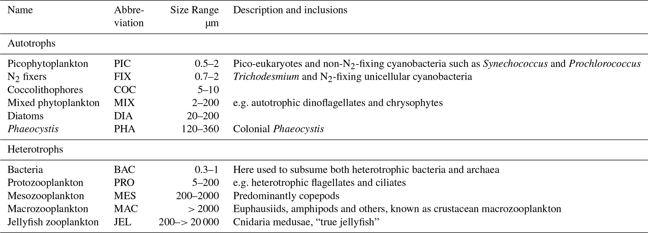
Models are useful tools to help understand the interactions of multiple complex drivers in the environment. This paper describes the addition of jellyfish to the Plankton Type Ocean Model v. 10 (PlankTOM10; Le Quéré et al., 2016) global ocean biogeochemical model, which we call PlankTOM11. PlankTOM10 represents explicitly 10 PFTs: six phytoplankton, one bacteria and three zooplankton (Le Quéré et al., 2016). The three zooplankton groups are protozooplankton (mainly heterotrophic flagellates and ciliates), mesozooplankton (mainly copepods) and macrozooplankton (as crustaceans, mainly euphausiids; see Table 1 for definitions). Jellyfish are therefore the fourth zooplankton group and 11th PFT in the PlankTOM model series. It introduces an additional trophic level to the ecosystem. To our knowledge, this is the first and only representation of jellyfish in a global ocean biogeochemical model at the time of writing. PlankTOM11 is used to help quantify global jellyfish biomass and the role of jellyfish for the global plankton ecosystem.
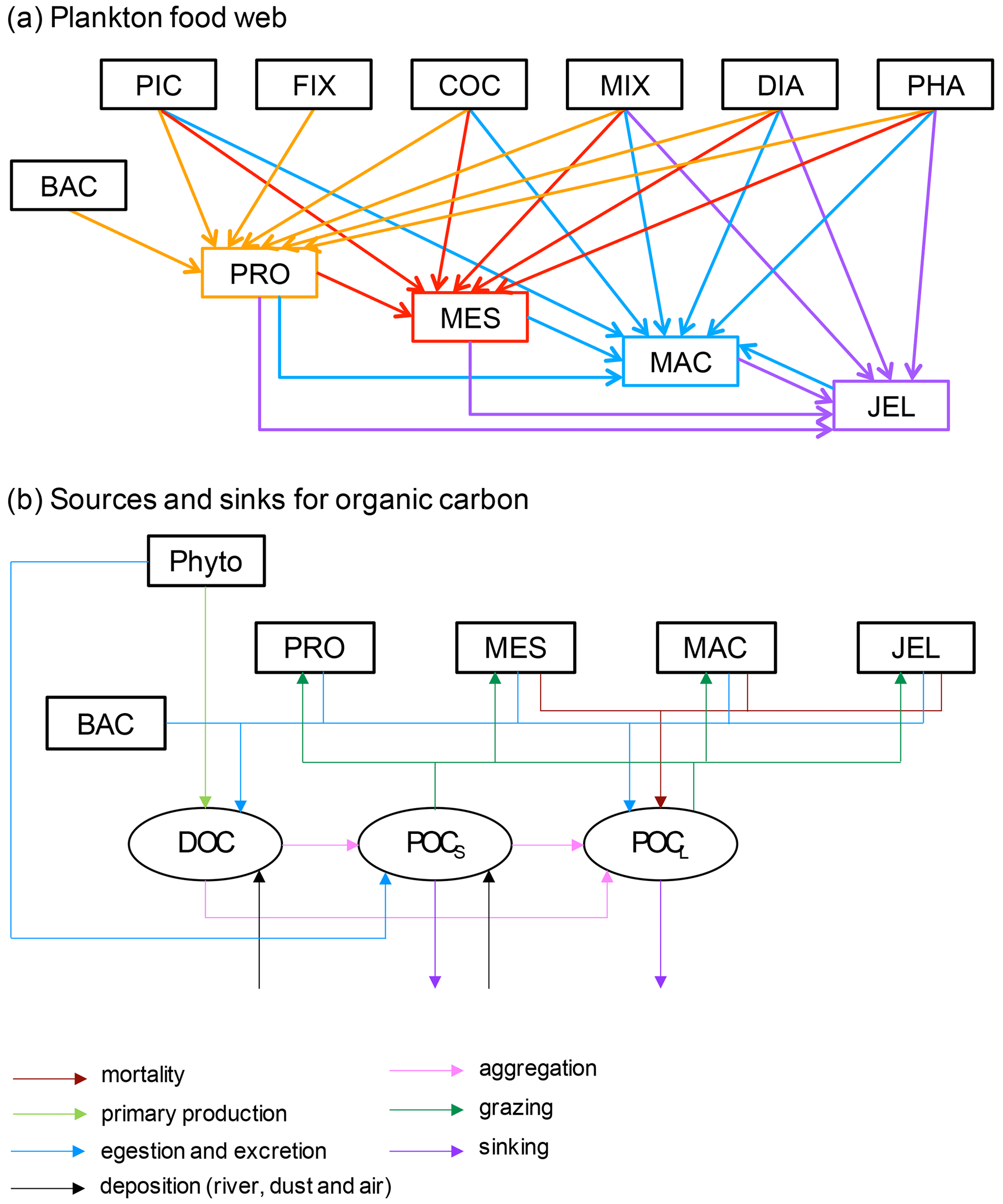
Figure 1Schematic representation of the PlankTOM11 marine ecosystem model (see Table 1 for PFT definitions). (a) The plankton food web; arrows represent the grazing fluxes by protozooplankton (orange), mesozooplankton (red), macrozooplankton (blue) and jellyfish zooplankton (purple). Only fluxes with relative preferences above 0.1 are shown (see Table 3). (b) Source and sinks for dissolved organic carbon (DOC) and small (POCS) and large (POCL) particulate organic carbon.
2.1 PLANKTOM11 model description
PlankTOM11 was developed starting from the 10 PFT version of the PlankTOM model series (Le Quéré et al., 2016) by introducing jellyfish as an additional trophic level at the top of the plankton food web (Fig. 1a). A full description of PlankTOM10 is published in Le Quéré et al. (2016), including all equations and parameters. Here we provide an overview of the model development, focussing on the parameterisation of the growth and loss rates of jellyfish and how these compare to the other macrozooplankton group. We also describe the update of the relationship used to describe the growth rate as a function of temperature and subsequent tuning. The formulation of the growth rate is the only equation that has changed since the previous version of the model (Le Quéré et al., 2016), although many parameters have been modified (Sect. 2.1.6).
PlankTOM11 is a global ocean biogeochemistry model that simulates plankton ecosystem processes and their interactions with the environment through the representation of 11 PFTs (Fig. 1). The 11 PFTs consist of six phytoplankton (picophytoplankton, nitrogen-fixing cyanobacteria, coccolithophores, mixed phytoplankton, diatoms and Phaeocystis), bacteria and four zooplankton (Table 1). Physiological parameters are fixed within each PFT; therefore, within-PFT diversity is not included. Spatial variability within PFTs is represented through parameter dependence on environmental conditions including temperature, nutrients, light and food availability.
The model contains 39 biogeochemical tracers, with full marine cycles of key elements carbon, oxygen, phosphorus and silicon, and simplified cycles of nitrogen and iron. There are three detrital pools: dissolved organic carbon (DOC), small particulate organic carbon (POCS) and large particulate organic carbon (POCL). The elements enter through riverine fluxes and are cycled and generated through the PFTs via feeding, faecal matter, messy eating and carcases (Fig. 1b; see Sect. 2.1.5 for detail; Buitenhuis et al., 2006, 2010, 2013a; Le Quéré et al., 2016). Model parameters are based on observations where available. A global database of PFT carbon biomass that was designed for model studies (Buitenhuis et al., 2013b) and global surface chlorophyll from satellite observations (SeaWiFS, Sea-viewing Wide Field-of-view Sensor) are used to guide the model developments.
The PlankTOM11 marine biogeochemistry component is coupled online to the global ocean general circulation model Nucleus for European Modelling of the Ocean version 3.5 (NEMO v3.5). We used the global configuration with a horizontal resolution of 2∘ longitude by a mean resolution of 1.1∘ latitude using a tripolar orthogonal grid. The vertical resolution is 10 m for the top 100 m, decreasing to a resolution of 500 m at 5 km depth, with a total of 30 vertical z levels (Madec, 2013). The ocean is described as a fluid using the Navier–Stokes equations and a nonlinear equation of state (Madec, 2013). NEMO v3.5 explicitly calculates vertical mixing at all depths using a turbulent kinetic energy model and sub-grid eddy-induced mixing. The model is interactively coupled to a thermodynamic sea-ice model (LIM version 2; Timmermann et al., 2005).
The temporal (t) evolution of zooplankton concentration (Zj), including the jellyfish PFT, is described through the formulation of growth and loss rates as follows:
(representing growth through grazing minus loss through grazing minus basal respiration)
(minus mortality).
For growth through grazing, g is the grazing rate by zooplankton Zj on food source Fk. This is a temperature-dependent Michaelis–Menten term that includes grazing preference (see Sect. 2.1.2). MGE is the modelled growth efficiency (Buitenhuis et al., 2010). For loss through grazing, g is the grazing of other zooplankton on Zj. For basal respiration, is the respiration rate at 0 ∘C, T is temperature and d is the temperature dependence of respiration (d10 = Q10). Mortality is the closure term of the model and is mostly due to predation by higher trophic levels that are represented by the model. m is the mortality rate at 0 ∘C, c is the temperature dependence of the mortality (c10 = Q10) and is the half saturation constant for mortality. ∑iPi is the sum of all PFTs, excluding bacteria, and is used as a proxy for the biomass of predators not explicitly included in the model. More details on each term are provided below, and parameter values are given in Tables 2 to 5.
Table 2Parameters used to calculate PFT-specific growth rate with a three-parameter fit (Eq. 3) in PlankTOM11.
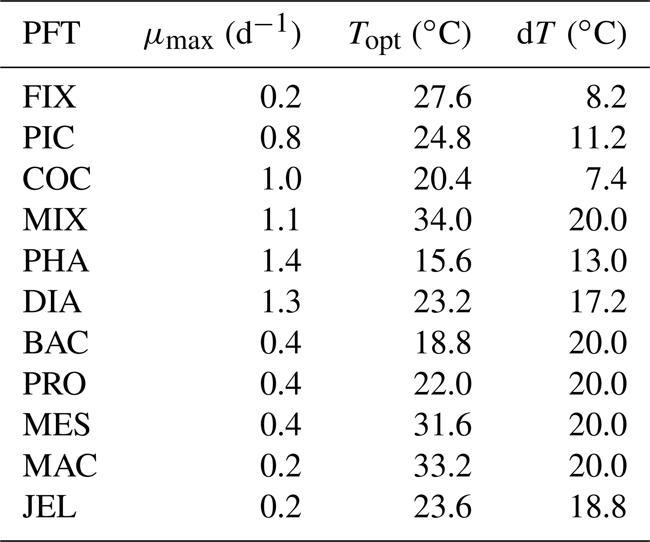
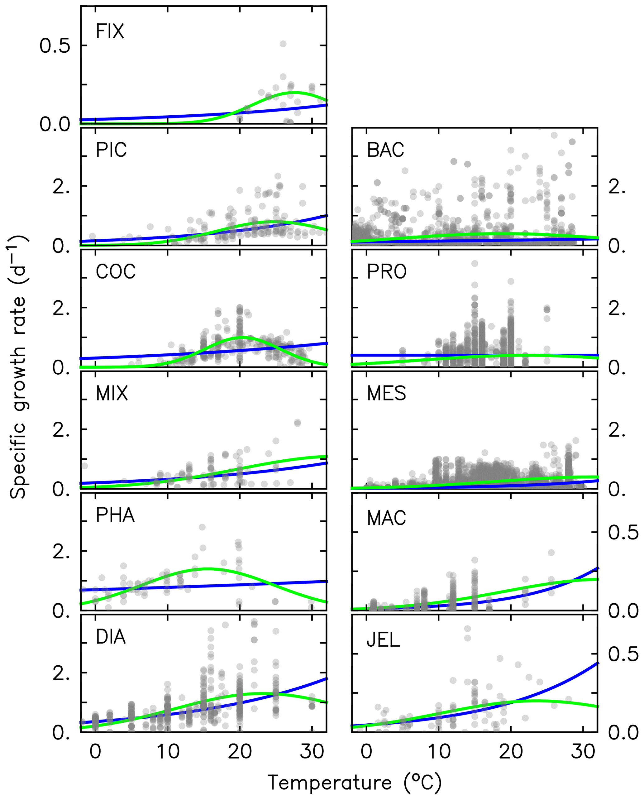
Figure 2Maximum growth rates for the 11 PFTs as a function of temperature from observations (grey circles). The three-parameter fit to data is shown in green, and the two-parameter fit is shown in blue, using the parameter values from Table 2. For full PFT names see Table 1. The R2 values for both fits to data are given in Appendix Table A2.
2.1.1 PFT growth
Growth rate is the trait that most distinguishes PFTs in models (Buitenhuis et al., 2006, 2013a). Jellyfish growth rates were compiled as a function of temperature from the literature (see Appendix Table A1). In previous published versions of the PlankTOM model, growth as a function of temperature (μT) was fitted with two parameters:
where μ0 is the growth at 0 ∘C, Q10 is the temperature dependence of growth derived from observations and T is the temperature (Le Quéré et al., 2016). Jellyfish growth rate is poorly captured by an exponential fit to temperature. To better capture the observations, the growth calculation has now been updated with a three-parameter growth rate, which produces a bell-shaped curve centred around an optimal growth rate at a given temperature (Fig. 2 and Table 2). The three-parameter fit is suitable for the global modelling of plankton, because it can represent an exponential increase if the data support this (Schoemann et al., 2005). The growth rate as a function of temperature (μT) is now defined by the optimal temperature (Topt), maximum growth rate (μmax) at Topt and the temperature interval (dT):
The available observations measure growth rate, but the model requires specification of the grazing rate (Eq. 1). Growth of zooplankton and grazing (gT) are related through the gross growth efficiency (GGE):
GGE is the portion of grazing that is converted to biomass. This was previously collated by Moriarty (2009) from the literature for crustacean and gelatinous macrozooplankton for the development of PlankTOM10. We extracted data for jellyfish from this collation (all scyphomedusae), which gave an average GGE of 0.29±0.27 and n=126 (Moriarty, 2009).
Table 3Relative preference, expressed as a ratio, of zooplankton for food (grazing) used in PlankTOM11. For each zooplankton, the preference ratio for diatoms is set to 1.
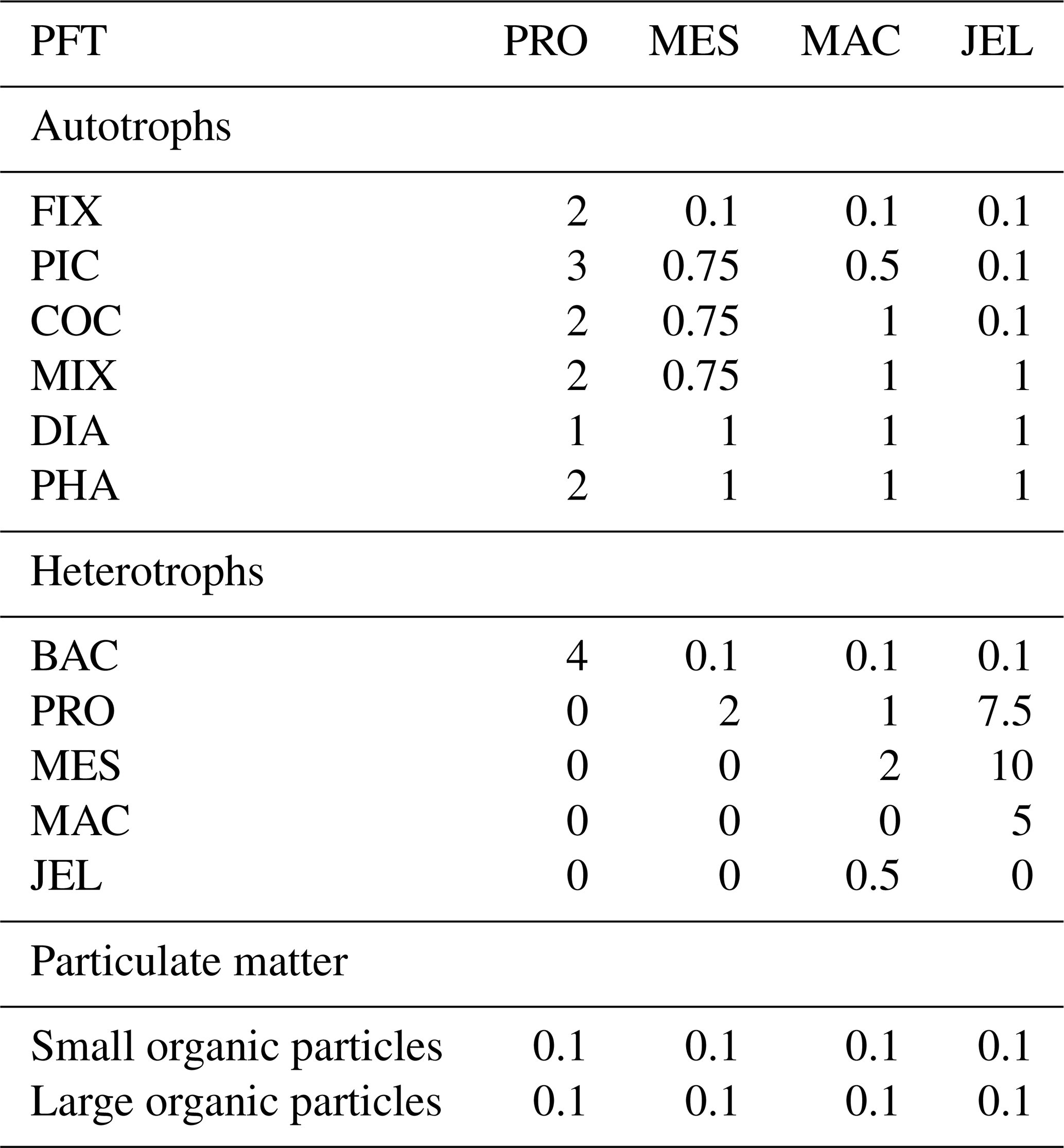
2.1.2 Jellyfish PFT grazing
The food web (and thus the trophic level of PFTs) is determined through grazing preferences. The relative preference of jellyfish zooplankton for the other PFTs was determined through a literature search (Colin et al., 2005; Costello and Colin, 2002; Flynn and Gibbons, 2007; Malej et al., 2007; Purcell, 1992, 1997, 2003; Stoecker et al., 1987; Uye and Shimauchi, 2005a; see Appendix Table A3 for further detail). The dominant food source was mesozooplankton (specifically copepods), followed by protozooplankton (most often ciliates) and then macrozooplankton (Table 3). There is little evidence for jellyfish actively consuming autotrophs. One of the few pieces of evidence is a gut content analysis where “unidentified protists… some chlorophyll bearing” were found in a small medusa species (Colin et al., 2005). Another is a study by Boero et al. (2007) which showed that very small medusae such as Obelia will consume bacteria and may consume phytoplankton. Studies on the diet of the ephyrae life-cycle stage are limited in comparison to those on medusa, but the literature does show evidence for ephyrae consuming protists and phytoplankton (Båmstedt et al., 2001; Morais et al., 2015). We assume that ephyrae are likely to have a higher preference for autotrophs, due to their smaller size as with the small medusa, but that this will have a minimal effect on the overall preferences and the biomass consumed, so preferences for autotrophs are kept low. Once the relative preference is established, the absolute value of the preference is tuned to improve the biomass of the different PFTs, as in Le Quéré et al. (2016). Table 3 shows the relative preference of jellyfish for its prey assigned in the model, along with the preferences of the other zooplankton PFTs. The zooplankton-relative preferences are based around a predator–prey size ratio, which by design is set to 1 for the zooplankton–diatom ratio. Preferences to other PFTs and to particulate carbon are then set relative to the preference for diatoms. The preference ratios are weighted using the global carbon biomass for each type against a total food biomass weighted mean (sum of all the PFTs), calculated from the MARine Ecosystem biomass DATa (MAREDAT) database, following the methodology used for the other PFTs (Buitenhuis et al., 2013a; Le Quéré et al., 2016). Zooplankton grazing is calculated using
where g is the grazing rate by zooplankton Zj on food source Fk as shown in Eq. (1), where μT is the growth rate of zooplankton (Eq. 3), p is the preference of the zooplankton for the food source (prey) and is the half saturation constant of zooplankton grazing. The parameter values for grazing used in the model are given in Table 4.
Table 4PlankTOM11 parameter values for macrozooplankton and jellyfish, with the associated equation.

2.1.3 Jellyfish PFT respiration
Previous analysis of respiration rates of jellyfish found that temperature manipulation experiments with Q10 values of > 3 were flawed, because the temperature was changed too rapidly (Purcell, 2009; Purcell et al., 2010). In a natural environment, jellyfish gradually acclimate to temperature changes, which has a smaller effect on their respiration rates. Purcell et al. (2010) instead collated values from experiments that measured respiration at ambient temperatures, providing a range of temperature data across different studies. They found that Q10 for respiration was 1.67 for Aurelia species (Purcell, 2009; Purcell et al., 2010). Moriarty (2009) collated a respiration dataset for zooplankton, including gelatinous zooplankton, using a similar selectivity as Purcell et al. (2010) for experimental temperature, feeding, time in captivity and activity levels. Jellyfish were extracted from the Moriarty (2009) dataset, which also included experiments on non-adult and non-Aurelia species medusae, unlike the Purcell et al. (2010) dataset. The relationship between temperature and respiration is heavily skewed by body mass (Purcell et al., 2010). The data were thus normalised by fitting to a general linear model (GLM) using a least squares cost function, to reduce the effect of body mass on respiration rates (Ikeda, 1985; Le Quéré et al., 2016).
where RR is the respiration rate, BM is the body mass, and T and RT are the observed temperature and associated respiration rate respectively. The parameter values were then calculated using R0=ea and Q, where e is the exponential function. The resulting fit to data is shown in Fig. 3. The parameter values for respiration used in the model are given in Table 4. Macrozooplankton respiration values are also given in Fig. 3 and Table 4, to provide a comparison to another zooplankton PFT of the most similar size available.
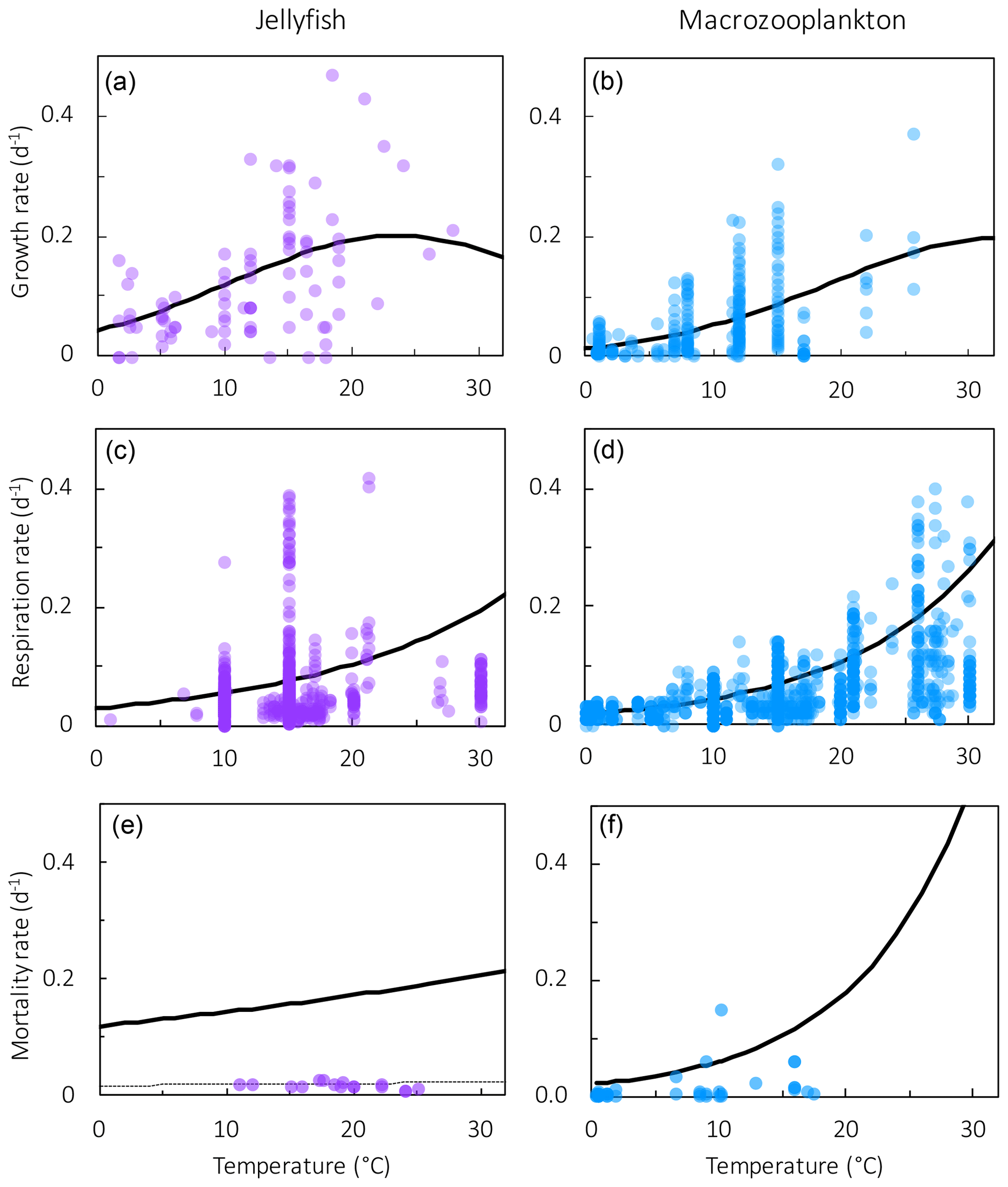
Figure 3Maximum growth rates (a, b), respiration rates (c, d) and mortality rates (e, f) for jellyfish (left; purple) and macrozooplankton (right; blue) PFTs as a function of temperature. The fit to data is shown in black, using the parameter values from Tables 2 and 4. Growth rates are the same as shown in Fig. 2 but on a different scale. For jellyfish mortality, the thin dashed line is the fit to data, and the solid line is the adjusted fit (Table 4).
2.1.4 Jellyfish PFT mortality
There are limited data on mortality rates for jellyfish, and to use mortality data from the literature on any zooplankton group, some assumptions must be made (Acevedo et al., 2013; Almeda et al., 2013; Malej and Malej, 1992; Moriarty, 2009; Rosa et al., 2013). These assumptions are that the population is in a steady state where mortality equals recruitment, reproduction is constant and mortality is independent of age (Moriarty, 2009). All models with zooplankton mortality rates follow these assumptions. In reality the mortality of a zooplankton population is highly variable. Steady states are balanced over a long period (if a population remains viable), reproduction is restricted to certain times of year and the early stages of life cycles are many times more vulnerable to mortality. Despite these assumptions, with the limited data on mortality rates, the larger uncertainty lies with the data rather than the assumptions (Moriarty, 2009). The half saturation constant for mortality ( in Eq. 1) is set to 20 µmol C L−1, which is the same as other zooplankton types, due to the lack of PFT-specific data. In the small number of data available and suitable for use in the model (16 data points from two studies), mortality ranged from 0.006–0.026 per day (Acevedo et al., 2013; Malej and Malej, 1992). Applying the exponential fit to these data gave a mortality rate at 0 ∘C (m in Eq. 1) of 0.018 per day. Sensitivity tests were carried out from this mortality rate due to low confidence in the value.
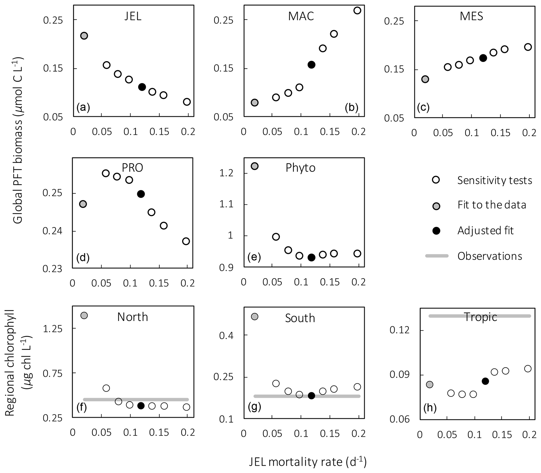
Figure 4Results from sensitivity tests on jellyfish mortality rates. The adjusted fit simulation used for PlankTOM11 is shown by the black filled circle, and the fit to the data simulation is shown by the grey filled circle; global mean PFT biomass (µmol C L−1) for 0–200 m depth (a–e) and regional mean surface chlorophyll concentration (µg chl L−1; f–h) are shown. For the regional mean chlorophyll, the observations are calculated from SeaWiFS. All data are averaged for 1985–2015, and between 30 and 55∘ latitude in both hemispheres: 140–240∘ E in the north and 140–290∘ E in the south (see Fig. 8). “Phyto” is the sum of all the phytoplankton PFTs.
Results from a subset of the sensitivity tests are shown in Fig. 4. The model was found to best represent a range of observations when jellyfish mortality was increased to 0.12 per day. The fit to data for mortality (μ0= 0.018) and the adjusted mortality (μ0=0.12) is shown in Fig. 3. This value was chosen based on expert judgement of the overall fit across multiple data streams. Although it was informed by the quantitative values in Table 6, the final choice required the balance of positive and negative performance that required expert judgement rather than a statistical number. Mortality rate values closer to 0.018 per day allowed jellyfish to dominate macro- and mesozooplankton, greatly reducing their biomass (Figs. 4 and 5). Low jellyfish mortality also resulted in higher chlorophyll concentrations than observed, especially in the high latitudes (Figs. 4 and 5; Bar-On et al., 2018; Buitenhuis et al., 2013b). The adjusted mortality rate used for PlankTOM11 may be accounting for several components missing from experimental data, including the impact of higher-trophic-level grazing in the Avecedo et al. (2013) study, which in copepods is 3–4 times higher than other sources of mortality (Hirst and Kiørboe, 2002), the greater vulnerability to mortality experienced during the early stages of the life cycle, and mortality due to parasites and viruses, especially during blooms (Pitt et al., 2014).

Figure 5Annual mean surface chlorophyll (µg chl L−1) and zooplankton carbon biomasses (µmol C L−1) of JEL, MAC, MES and PRO for adjustment of JEL mortality for the simulation with a 0.02 mortality rate per day (left) and the adjusted fit simulation with a 0.12 mortality rate per day (right) used in PlankTOM11. Results are shown for the surface box (0–10 m) and averaged for 1985–2015.
PlankTOM11 uses a mortality rate for jellyfish that is much higher than the limited observations (Figs. 4 and 5). Lower jellyfish mortality is likely to be more representative of adult life stages, as jellyfish experience high mortality during juvenile life stages, especially as planula larvae and during settling (Lucas et al., 2012). The limited observations of jellyfish mortality are from mostly adult organisms, which may explain the dominance of jellyfish in the model when parameterised with the observed mortality fit. The higher mortality used for this study may be more representative of an average across all life stages. Experimental jellyfish mortality is also likely to be lower than in situ mortality due to factors such as senescence post-spawning and bloom conditions increasing the prevalence of disease and parasites and thus increasing mortality (Mills, 1993; Pitt et al., 2014). Using a higher mortality for this study is therefore deemed reasonable.
2.1.5 Organic carbon cycling through the plankton ecosystem
In PlankTOM11, the growth of phytoplankton modifies dissolved inorganic carbon into DOC, which then aggregates into POCS and POCL (Fig. 1b). POCS is also generated from protozooplankton egestion and excretion and is consumed through grazing by all zooplankton. POCL is also generated by aggregation from POCS, egestion and excretion by all zooplankton; it is generated from the mortality of mesozooplankton, macrozooplankton and jellyfish and is consumed through grazing by all zooplankton. The portion of POCS and POCL which is not grazed sinks through the water column and is counted as export production at 100 m (Fig. 1b). The sinking speed of POCS is 3 m d−1, and the sinking speed of POCL varies, depending on the concentration of ballast and the resulting particle density. Proto-, meso- and macrozooplankton excretion is largely in the form of particulate and solid faecal pellets, while this makes up very little of jellyfish excretion. Jellyfish instead produce and slough off mucus as part of their feeding mechanism (Pitt et al., 2009), which is represented in the model in the same way as the faecal pellet excretion, i.e. as a fraction of unassimilated grazing contributing to POCL.
2.1.6 Additional tuning
Following the change to the growth rate formulation (from Eqs. 2 to 3), all PFT growth rates are lower compared to the published version of PlankTOM10 (Le Quéré et al., 2016), but the change is largest for Phaeocystis, diatoms, bacteria and protozooplankton (Fig. 2). Further tuning is carried out to rebalance the total biomass among phytoplankton PFTs following the change in formulation. The tuning included increasing the grazing ratio preference of mesozooplankton for Phaeocystis and the grazing ratio preference of protozooplankton for picophytoplankton within the limits of observations. Tuning also included increasing the half saturation constant of the phytoplankton Phaeocystis, picophytoplankton and diatoms for iron. The tuning resulted in a reduction of Phaeocystis biomass and an increase in diatom biomass, without disrupting the rest of the ecosystem. Diatom respiration was also increased to reduce their biomass towards observations. Finally, bacterial biomass was increased closer to observations by reducing the half saturation constant of bacteria for dissolved organic carbon and reducing the maximum bacteria uptake rate. See Appendix Table A4 for the parameter values before and after tuning.
Table 5Changes to non-jellyfish PFT parameters across the PlankTOM simulations. PlankTOM10LQ16 is the latest published version of PlankTOM with 10 PFTs (Le Quéré et al., 2016), while PlankTOM10 is the simulation from this study.

As shown in Eq. (1), there is a component in the mortality of zooplankton to represent predation by organisms not included in the model. The jellyfish PFT is a significant grazer of macrozooplankton and mesozooplankton (Table 3). To account for this additional grazing, the mortality term for macrozooplankton and the respiration term for mesozooplankton were reduced compared to model versions where no jellyfish are present (Table 5). Respiration is reduced in place of mortality for mesozooplankton as their mortality term had already been reduced to zero to account for predation by macrozooplankton (Le Quéré et al., 2016). The jellyfish PFT is also a significant grazer of protozooplankton; however, following the adjustment of protozooplankton grazing on picophytoplankton to account for changes to the growth rate formulation and the low sensitivity of protozooplankton to jellyfish mortality (Fig. 4), additional changes to protozooplankton parameters were found to be unnecessary.
2.1.7 Model simulations
The PlankTOM11 simulations are run from 1920 to 2015, forced by meteorological data including daily wind stress, cloud cover, precipitation and freshwater riverine input from NCEP/NCAR reanalysed fields (Kalnay et al., 1996). The simulations start with a 28-year spin-up for 1920–1948 where the meteorological conditions for year 1980 are used, looping over a single year. Year 1980 is used as a typical average year, as it has no strong El Niño/La Niña, as in Le Quéré et al. (2010). Furthermore, because of the greater availability of weather data (including by satellite) in 1980 compared to 1948, the dynamical fields are generally more representative of small-scale structures than the earlier years. There is a small shock to the system at the start of meteorological forcing, but this stabilises within a few years and decades before the model output is used for analysis. Tests of different spin-up years were carried out in Le Quéré et al. (2010), including both 1948 and 1980, with little impact on trends generally. The spin-up is followed by interannually varying forcing for actual years from 1948–2015. All analysis is carried out on the average of the last 31-year period of 1985–2015. PlankTOM11 is initialised with observations of dissolved inorganic carbon (DIC) and alkalinity (Key et al., 2004) after removing the anthropogenic component for DIC (Le Quéré et al., 2010), NO3, PO4, SiO3, O2, temperature and salinity from the World Ocean Atlas (Antonov et al., 2010).
Two further model simulations were carried out in order to better understand the effect of adding the jellyfish PFT. The first simulation sets the jellyfish growth rate to 0, so it replicates the model set-up with 10 PFTs in Le Quéré et al. (2016), which is here called PlankTOM10LQ16, but it includes the updated growth formulation (Sect. 2.1.1) and additional tuning (Sect. 2.1.5). The simulation is labelled “PlankTOM10” in the figures. This simulation is otherwise identical to PlankTOM11 except for the mortality term for macrozooplankton and the respiration term for mesozooplankton, which were initially returned to PlankTOM10LQ16 values, to account for the lack of predation by jellyfish. Macrozooplankton mortality was then tuned down from the PlankTOM10LQ16 value, from 0.02 to 0.012, to account for the change to the growth calculation (Table 5). The second additional simulation is carried out to test the addition of an 11th PFT in comparison to the addition of jellyfish as the 11th PFT. This is done by parameterising the jellyfish PFT identically to the macrozooplankton PFT in PlankTOM11 so that there are 11 PFTs active, with two identical macrozooplankton. This simulation is called PlankTOM10.5. The two macrozooplankton in PlankTOM10.5 have mutual predation, where they prey on each other, while the macrozooplankton in PlankTOM10 have no preference for themselves. Subsequently, macrozooplankton mortality in PlankTOM10.5 is kept the same as PlankTOM11 (Table 5) to account for the mutual predation. Otherwise, these simulations were identical to PlankTOM11.
2.2 Jellyfish biomass observations
MARine Ecosystem biomass DATa (MAREDAT) is a database of global ocean plankton abundance and biomass, which is harmonised to common units and is available online as open-source data (Buitenhuis et al., 2013b). The MAREDAT database is designed to be used for the validation of global ocean biogeochemical models. MAREDAT contains global quantitative observations of jellyfish abundance and biomass as part of the generic macrozooplankton group (Moriarty et al., 2013). The jellyfish subset of data has not been analysed independently yet.
For this study, all MAREDAT records under the group Cnidaria medusae (true jellyfish) were extracted from the macrozooplankton group (Moriarty et al., 2013) and examined. The taxonomic level within the database varies from phylum down to species. The data cover the period from August 1930 to August 2008 and contain abundance (individuals m−3, n=107 156) and carbon biomass (µg C L−1, n=3406). The carbon biomass data are used over the abundance data despite the fewer data available, as they can be directly compared to PlankTOM11 results. Carbon biomass is calculated from wet-weight to dry-weight conversion factors for species where data records are sufficient (Moriarty et al., 2013). The data were collected at depth ranging from 0 to 2442 m. The majority of the data (97 %) was collected in the top 200 m with an average depth of 44 m (±32 m). Data from the top 200 m are included in the analysis. The original un-gridded biomass data were binned into boxes at monthly resolution, as in Moriarty et al. (2013), reducing the number of gridded biomass data points to 849.
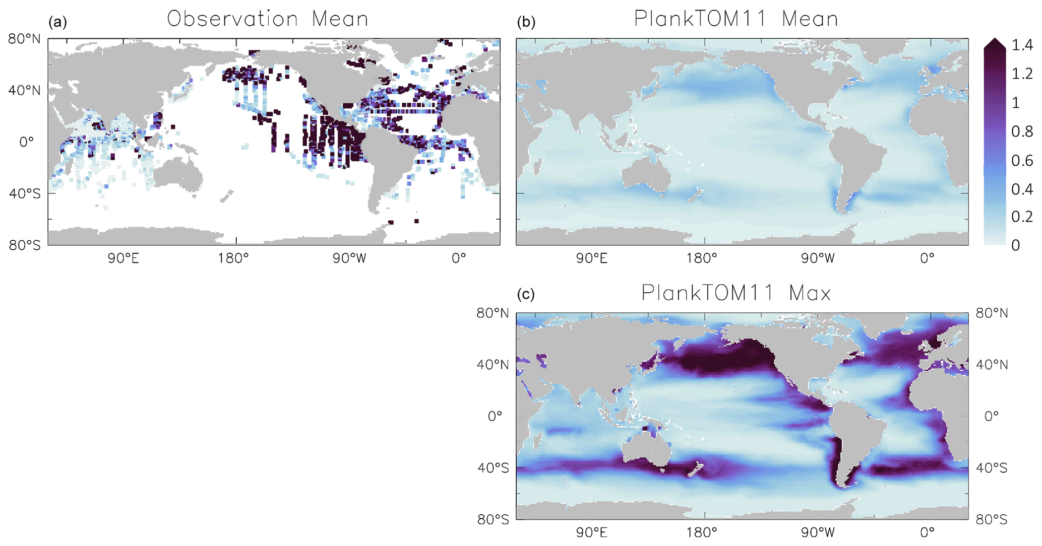
Figure 6Jellyfish carbon biomass (µmol C L−1) in PlankTOM11 and in observations from the Jellyfish Database Initiative (Luo et al., 2020). PlankTOM11 results (b, c) are the mean and maximum biomass from monthly climatologies. Observations (a) are the mean biomass; areas with no observations are in white. Observations are on a grid and are plotted using a three-cell averaging filler for visual clarity. All data are for 0–200 m. The gridded observation data are only available as a mean over time and depth (Luo et al., 2020). Due to the patchy nature of the observations in depth and time, the mean may be skewed high or low, while the model is sampled across the full time and depth.
In MAREDAT, jellyfish biomass data are only present in the Northern Hemisphere, which is likely to skew the data. Another caveat against the data is that a substantially smaller frequency of zeros is reported for biomass than for abundance. Under-reporting of zero values will increase the average, regardless of the averaging method used. Biomass observations from other global studies (Bar-On et al., 2018; Lucas et al., 2014; Luo et al., 2020) are used conjunctly with the global jellyfish biomass calculated here because of the poor spatial coverage.
To compare to the other PFTs within the MAREDAT database, global jellyfish biomass was calculated according to the methods in Buitenhuis et al. (2013b). Buitenhuis et al. (2013b) calculate a biomass range, using the median as the minimum and the arithmetic mean (AM) as the maximum. The jellyfish zooplankton biomass range in MAREDAT was calculated as 0.46–3.11 PgC, with the median jellyfish biomass almost as high as the microzooplankton and higher than meso- and macrozooplankton (Buitenhuis et al., 2013b). The jellyfish biomass range calculated here is used to validate the new jellyfish component in the PlankTOM11 model.
3.1 Jellyfish biomass
The global jellyfish biomass estimated by various studies gives a range of results: 0.1 PgC (Bar-On et al., 2018), 0.32±0.49 PgC (Lucas et al., 2014), 0.29±0.56 PgC (Luo et al., 2020, updated from Lucas et al., 2014) and 0.46–3.11 PgC calculated in this study (Sect. 2.2). Jellyfish biomass in PlankTOM11 is within the range but towards the lower end of observations at 0.13 PgC, with jellyfish accounting for 16 % of the total zooplankton biomass (Table 6). When the modelled biomass was tuned to match the higher observed biomass by adjusting the mortality rate, jellyfish dominate the entire ecosystem significantly, reducing levels of the other zooplankton and increasing chlorophyll above observations for the Northern Hemisphere and Southern Hemisphere (Figs. 4 and 5).
Table 6Global mean values for rates and biomass from observations and the PlankTOM11 and PlankTOM10 models averaged over 1985–2015. In parenthesis is the percentage share of the plankton type of the total phytoplankton or zooplankton biomass. The percentage share of mixed phytoplankton is not included, as there are no mixed-phytoplankton observations; therefore, the phytoplankton percentages are of total phytoplankton minus mixed phytoplankton. References for observations are given in Appendix Table A5.

PlankTOM11 generally replicates the patterns of jellyfish biomass with observations. High biomass occurs at around 50–60∘ N across the oceans, with the highest biomass in the North Pacific. PlankTOM11 also replicates low biomass in the Indian Ocean, and the eastern half of the tropical Pacific shows higher biomass compared to other open ocean areas in agreement with patterns in observations (Fig. 6; Lucas et al., 2014; Luo et al., 2020). However, PlankTOM11 underestimates the high jellyfish biomass in the tropical Pacific (Fig. 6). Most of the data informing the jellyfish parameters are from temperate species, so the model will better represent higher latitudes compared to lower latitudes. This is likely responsible for some of the underestimation of biomass in this region. The competition of jellyfish with macrozooplankton also plays a role (see Sect. 3.3 for further discussion). The lack of biomass observations around 40∘ S makes it difficult to determine if the peak in jellyfish biomass in PlankTOM11 at this latitude is representative of reality. The maximum biomass in the Southern Hemisphere is mostly around coastal areas, i.e. South America and southern Australia (Fig. 6). This is expected from reports and papers on jellyfish in these areas (Condon et al., 2013; Purcell et al., 2007, and references therein). A prevalence of jellyfish in coastal areas is apparent (Fig. 6), in line with observations (Lucas et al., 2014; Luo et al., 2020), even without any specific coastal advantages for jellyfish in the model (see macrozooplankton in Le Quéré et al., 2016). However, PlankTOM11 underestimates the range of observations in the top 200 m (Fig. 6). PlankTOM11 overestimates the minimum values and underestimates the maximum values. However, part of this discrepancy may be due to under-sampling in the observations. A key caveat in jellyfish data is that the data are not uniformly distributed spatially or temporally and not proportionally distributed between various biomes of the ocean, with collection efforts skewed to coastal regions and the Northern Hemisphere (MAREDAT; Lilley et al., 2011; Lucas et al., 2014; Luo et al., 2020). This sampling bias and the sampling methods also tend to favour larger, less delicate species, which are often scyphomedusae with a meroplanktonic life cycle.
Jellyfish are characterised by their bloom and bust dynamic, resulting in patchy and ephemeral biomass. The mean to max biomass ratio of observations (MAREDAT) was compared to the same ratio for PlankTOM11 to assess the replication of this characteristic. The observations give a wide range of ratios depending on the type of mean used. The PlankTOM11 ratio falls within this range but towards the lower end (Table 7). PlankTOM11 replicates some of the patchy and ephemeral biomass of jellyfish.
Table 7Jellyfish biomass globally from observations (MAREDAT) and PlankTOM11. Three types of mean are given for the observations; Med is the median, AM is the arithmetic mean and GM is the geometric mean. The ratios are all scaled to mean = 1. All units are in µg C L−1.
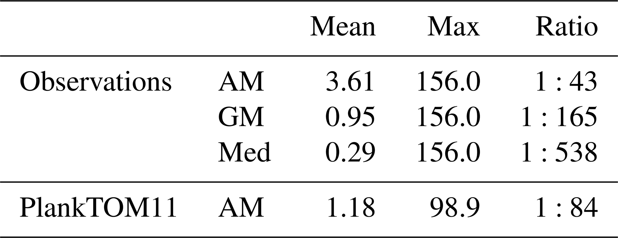
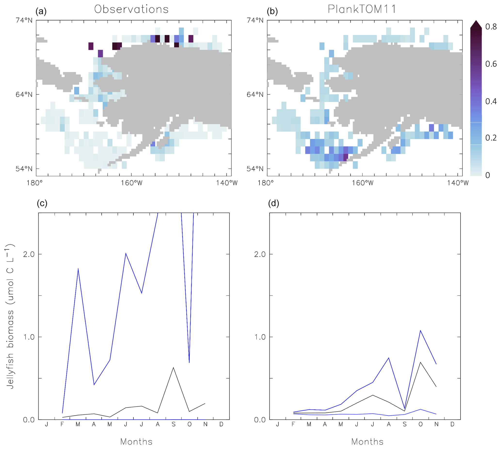
Figure 7Carbon biomass of jellyfish (µmol C L−1) from MAREDAT observations (a, c) and PlankTOM11 (b, d) for the coast of Alaska (the region with the highest density of observations). Panels (a, b) show the mean jellyfish biomass, and panels (c, d) the seasonal jellyfish biomass, with the monthly mean in black and the monthly minimum and maximum in blue. Observations and PlankTOM11 results are for 0–150 m, as the depth range where > 90 % of the observations occur. No observations were available for January or December.
Jellyfish biomass in MAREDAT has poor global spatial coverage. The region around the coast of Alaska has the highest density of observations and is used here to evaluate the mean, range and seasonality of the carbon biomass of jellyfish as represented in PlankTOM11. The gridded jellyfish observations from Luo et al. (2020; see Fig. 6) are available as a mean over time and depth, so they cannot be used to evaluate range or seasonality. Spatially, the observations peak around the north coast of Alaska, while PlankTOM11 peaks around the south coast (Fig. 7). This difference is likely due to the lack of small-scale physical processes in the model due to the relatively coarse model resolution. PlankTOM11 reproduces the observed mean jellyfish biomass around the coast of Alaska (0.16 compared to 0.13 µmol C L−1), but it underestimates the maximum and spread of the observations (Table 8). The spatial patchiness is somewhat replicated in PlankTOM11, although with a smaller variation (Fig. 7). PlankTOM11 replicates the mean seasonal shape and biomass of jellyfish with a small peak over the summer followed by a large peak in September in the observations and in October in PlankTOM11 (Fig. 7). Overall, PlankTOM11 replicates the mean but underestimates the maximum biomass and temporal patchiness of the observations (Fig. 7 and Table 8).
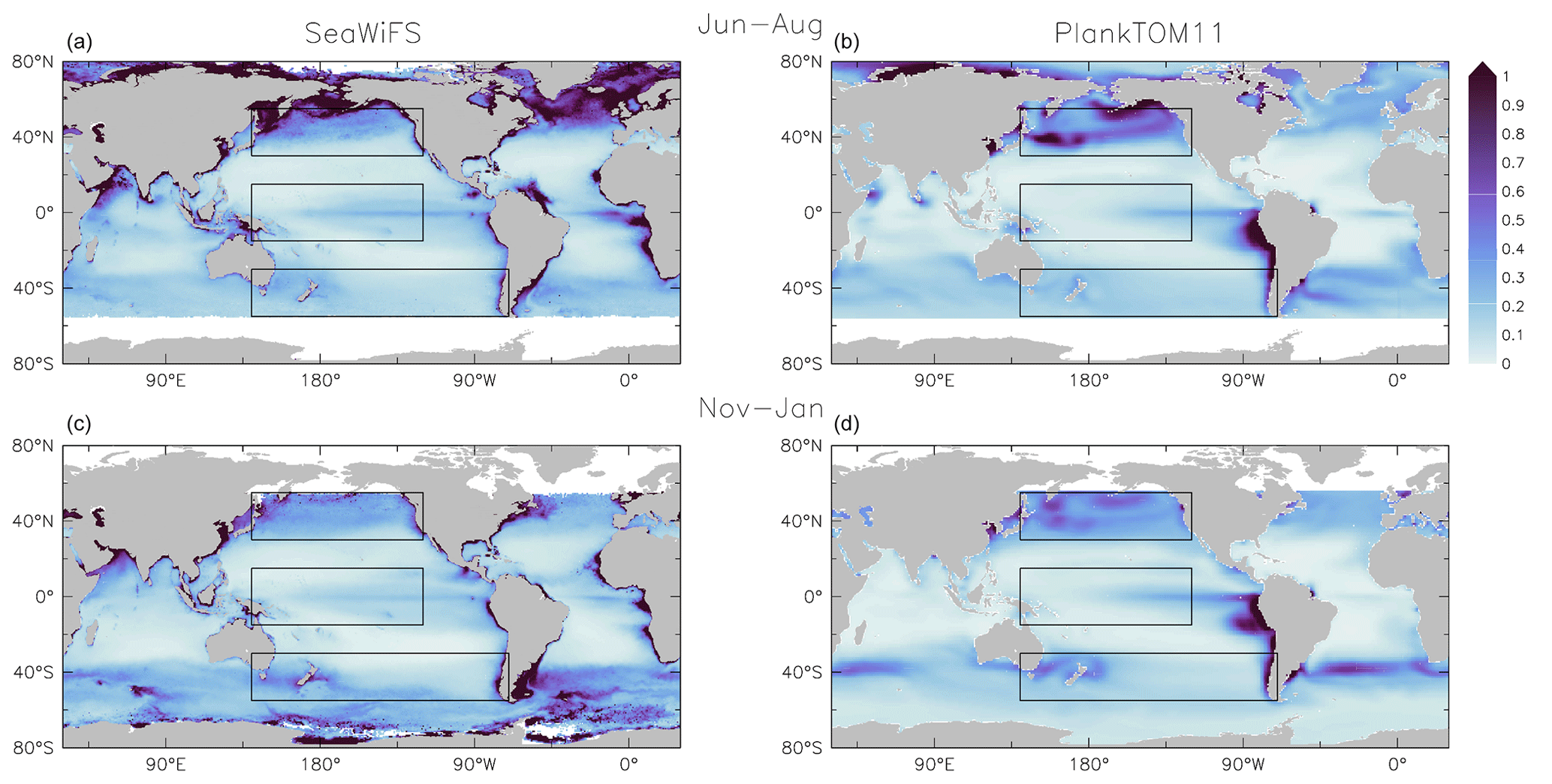
Figure 8Surface chlorophyll (µg chl L−1) averaged for June to August (a, b) and November to January (c, d). Panels show observations from the SeaWiFS (a, c) satellite and results from PlankTOM11 (b, d). Observations and model are averaged for 1997–2006. The black boxes show the Pacific northern, tropical and southern regions used in Figs. 4 and 9.
3.2 Ecosystem properties of PLANKTOM11
PlankTOM11 reproduces the main characteristics of surface chlorophyll observations, with high chlorophyll concentration in the high latitudes, low concentration in the subtropics and elevated concentrations around the Equator (Fig. 8). PlankTOM11 also reproduces higher chlorophyll concentrations in the northern Pacific compared to the southern Pacific (Fig. 9) and higher concentrations in the southern Atlantic compared to the southern Pacific Ocean (Fig. 8). Overall the model underestimates chlorophyll concentrations, as is standard with models of this type (Le Quéré et al., 2016), particularly in the central and northern Atlantic. PlankTOM11 also captures the seasonality of chlorophyll, with concentrations increasing in summer compared to the winter for each hemisphere (Fig. 8).
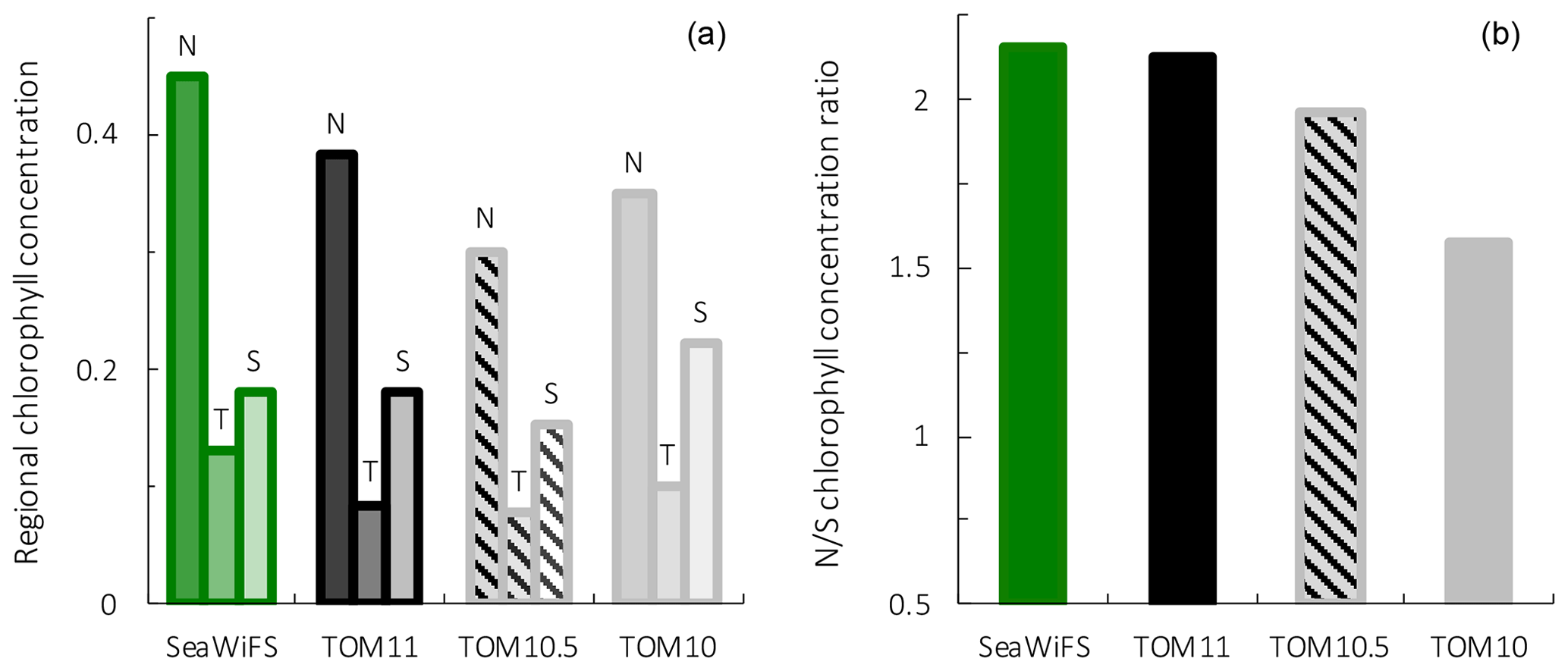
Figure 9Surface chlorophyll for observations from the SeaWiFS satellite, PlankTOM11, PlankTOM10.5 and PlankTOM10. Regional chlorophyll concentration is in µg chl L−1 (a) for the northern (N), tropical (T) and southern (S) Pacific Ocean regions shown in Fig. 8 and the N/S chlorophyll concentration ratio (b). Observations and model are averaged for 1997–2006.
To assess the effect of adding jellyfish to PlankTOM, two additional simulations were conducted: PlankTOM10 where jellyfish growth is set to zero and PlankTOM10.5 where all jellyfish parameters are set equal to macrozooplankton parameters (Sect. 2.1.6). The two simulations show similar spatial patterns of surface chlorophyll to PlankTOM11 but different concentration levels. PlankTOM11 closely replicates the chlorophyll ratio between the north and south Pacific with a ratio of 2.12 compared to the observed ratio of 2.16 (Fig. 9). PlankTOM10 and PlankTOM10.5 underestimate the observed ratio with ratios of 1.57 and 1.96 respectively (Fig. 9). Adding an 11th PFT improves the chlorophyll ratio; however, the regional chlorophyll concentrations for PlankTOM10.5 are a poorer match to the observations than PlankTOM11, especially in the north (Fig. 9). PlankTOM10 overestimates the observed chlorophyll concentration in the south (0.22 and 0.18 respectively; Fig. 9). All three simulations underestimate chlorophyll concentration in the tropics compared to observations (Fig. 9). The north-to-south chlorophyll ratio metric was developed by Le Quéré et al. (2016) as a simple method to quantify model performance for emergent properties, focussing on the Pacific Ocean as the area where this ratio is most pronounced in the observations. These simulations further support the suggestion by Le Quéré et al. (2016) that the observed distribution of chlorophyll in the north and south is a consequence of trophic balances between the PFTs and improves with increasing plankton complexity.
PlankTOM11 underestimates primary production by 10 PgC yr−1, which is similar to the underestimation in PlankTOM10LQ16 of 9 PgC yr−1. As suggested by Le Quéré et al. (2016), this may be due to the model only representing highly active bacteria, which is unchanged between the model versions, while observed biomass is also from low-activity bacteria and ghost cells. Export production and N2 fixation are within the observational range, and CaCO3 export is slightly overestimated (Table 6).
In PlankTOM11 each PFT shows a unique spatial distribution in carbon biomass (Fig. 5). The total biomass of phytoplankton is within the range of observations, but the partitioning of this biomass between phytoplankton types differs from observations (Table 6). PlankTOM11 is dominated by mixed phytoplankton and coccolithophores, together making up 47 % of the total phytoplankton biomass. Diatoms and Phaeocystis are the next most abundant and fall within the observed range, followed by picophytoplankton with around half the observed biomass (Table 6). The observations are dominated by picophytoplankton, followed by Phaeocystis and diatoms (Table 6). The modelled mixed phytoplankton is likely taking up the ecosystem niche of picophytoplankton. Coccolithophores are overestimated by a factor of 10 and may also be filling the ecosystem niche of picophytoplankton in the model (Table 6). The phytoplankton community composition changed from PlankTOM10LQ16 to PlankTOM11, with some phytoplankton types moving closer to observations and some moving further away. For example, for N2 fixers PlankTOM11 is in line with the upper end of observations at 8 %, while PlankTOM10 and PlankTOM10LQ16 overestimate N2 fixers (10 % and 11 % respectively). For picophytoplankton, PlankTOM10LQ16 is within the range of observations at 38 %, while PlankTOM11 and PlankTOM10 underestimate the community share of picophytoplankton (17 % and 20 % respectively). For Phaeocystis, all three simulations underestimate the community share, but PlankTOM11 and PlankTOM10 (both 22 %) are closer to the lower end of observations (27 %) than PlankTOM10LQ16 (15 %; Table 6; Le Quéré et al., 2016). Overall, the difference between PlankTOM10LQ16 and PlankTOM11 is greater than the difference between PlankTOM10 and PlankTOM11, suggesting that the change to growth of PFTs had a larger effect on phytoplankton community composition than the addition of jellyfish. This is expected, as the growth change directly effects each PFT and model results are sensitive to PFT growth rates (Buitenhuis et al., 2006, 2010). Jellyfish affect phytoplankton community composition, but the effect is small.
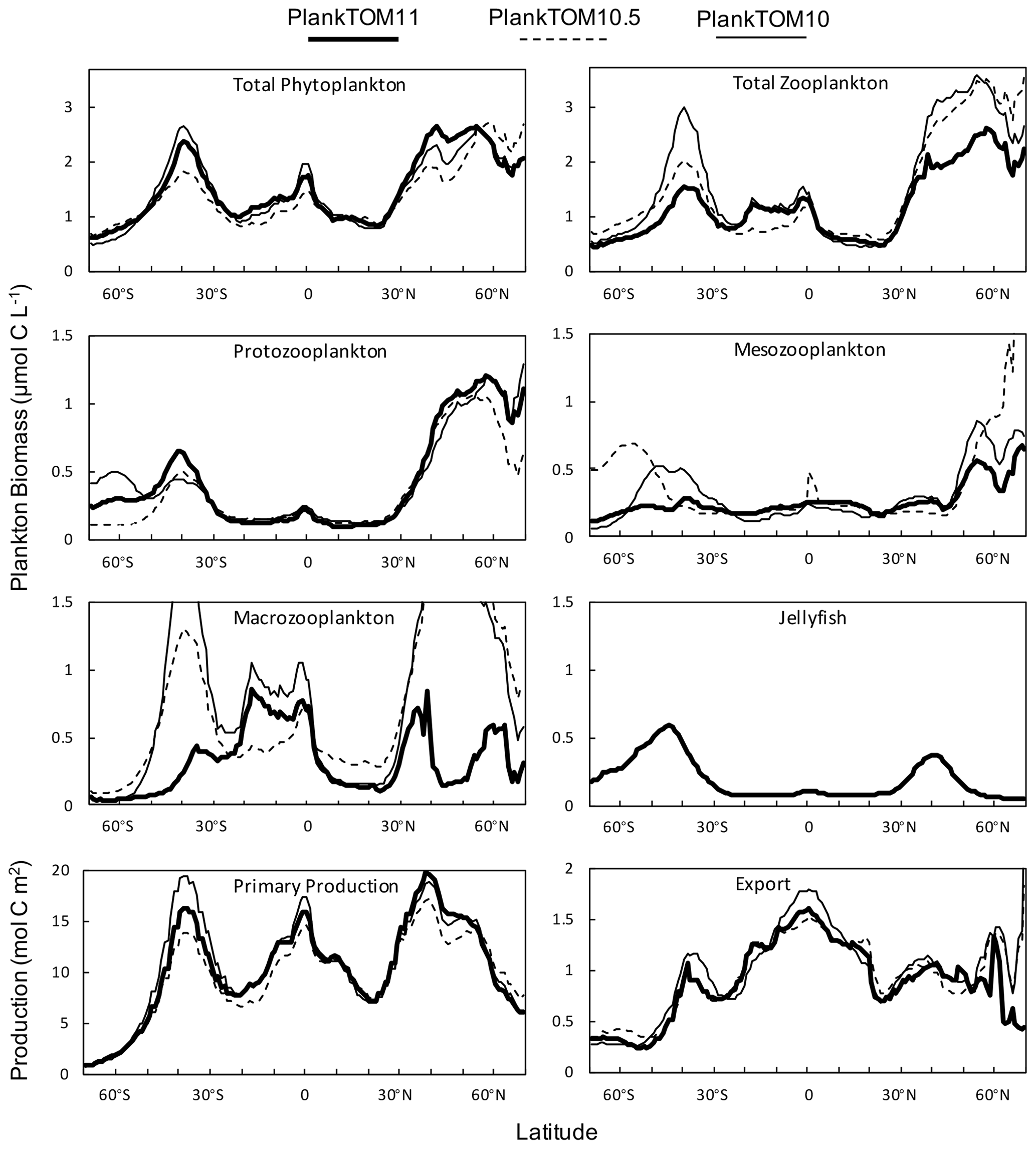
Figure 10Zonal mean distribution for the PlankTOM11, PlankTOM10.5 and PlankTOM10 simulations. All plankton biomass data are for the surface box (0–10 m). For PlankTOM10.5, the MAC PFT has been summed with the 11th PFT that duplicates MAC. The bottom panels are the zonal mean distribution of primary production, integrated over the top 100 m, and export production at 100 m. All data are averaged for 1985–2015.
3.3 Role of jellyfish in the plankton ecosystem
Macrozooplankton exhibit the largest change in biomass between the three simulations, followed by mesozooplankton (Fig. 10). This is despite the higher preference of jellyfish grazing on mesozooplankton (ratio of 10) than on macrozooplankton (ratio of 5; Table 3). The central competition for resources between jellyfish and macrozooplankton is that they both preferentially graze on mesozooplankton, then on protozooplankton, although macrozooplankton have a lower preference ratio for zooplankton than jellyfish, as more of their diet is made up by phytoplankton (Table 3). In simple terms, this means that for two equally sized populations of jellyfish and macrozooplankton, jellyfish would consume more meso- and protozooplankton than would be consumed by macrozooplankton. However, predator biomass, prey biomass and the temperature dependence of grazing interact to affect the rate of consumption (Eq. 5). The greatest difference in PFT biomass, especially macrozooplankton biomass, between simulations occurs in latitudes higher than 30∘ where jellyfish biomass is highest (Fig. 10). In the tropics, jellyfish have a low impact on the ecosystem due to their low biomass in this region (Figs. 6 and 10).
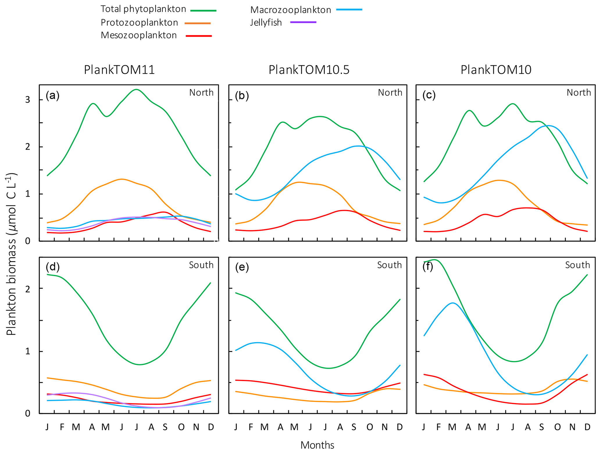
Figure 11Seasonal surface carbon biomass (µmol C L−1) of total phytoplankton PFTs, protozooplankton, mesozooplankton, macrozooplankton and jellyfish. For PlankTOM10.5, the MAC PFT has been summed with the 11th PFT that duplicates MAC. Panels shown PFT biomass for PlankTOM11 (a, d), PlankTOM10.5 (b, e) and PlankTOM10 (c, f) for two regions; the north, 30–70∘ N (a–c), and the south 30–70∘ S (d–f), across all longitudes. All data are averaged for 1985–2015.
The seasonality of the PFTs in each simulation is shown in Fig. 11 for 30–70∘ north and south, as the regions with the greatest differences between simulations (Fig. 10). In PlankTOM10, macrozooplankton represent the highest trophic level. The addition of another PFT at the same or at a higher trophic level (PlankTOM10.5 and PlankTOM11 respectively) reduces the biomass of the macrozooplankton through a combination of competition and low-level predation (Figs. 10 and 11). For PlankTOM10.5 results, macrozooplankton is summed with the 11th PFT (identical to macrozooplankton in this simulation). The addition of this 11th PFT at the same trophic level reduces the biomass of the macrozooplankton (Figs. 10 and 11), despite the macrozooplankton mortality being reduced from PlankTOM10 to PlankTOM10.5 (Table 5), which would be expected to increase macrozooplankton biomass. However, the low level of mutual predation between the two macrozooplankton PFTs slightly reduces their overall biomass. This reduction in biomass mostly occurs during the autumn macrozooplankton bloom, where the peak is reduced from PlankTOM10 to PlankTOM10.5, while the winter to spring biomass is similar across the two simulations (Fig. 11). The drop in mesozooplankton respiration from PlankTOM10 to PlankTOM10.5 (Table 5) lowers the rate of respiration, especially at lower temperatures. This likely accounts for the increase in PlankTOM10.5 mesozooplankton biomass at higher latitudes (Fig. 10). The addition of jellyfish changes the zooplankton with the highest biomass from macrozooplankton to protozooplankton and reduces the biomass of mesozooplankton, in both the north and south (Fig. 11). However, the impact on the biomass of mesozooplankton and protozooplankton is small, despite mesozooplankton being the preferential prey of jellyfish, followed by protozooplankton. The small impact of jellyfish on mesozooplankton and protozooplankton biomass may be due to trophic cascade effects where jellyfish reduce the biomass of macrozooplankton, which reduces the predation pressure of macrozooplankton on meso- and protozooplankton whilst jellyfish simultaneously provide an additional predation pressure on meso- and protozooplankton. The decrease in predation by macrozooplankton may be compensated for by the increase in predation by jellyfish, resulting in only a small change to the overall biomass of mesozooplankton and protozooplankton.
In PlankTOM11, there is a clear distinction between the biomass in the north and south, with higher biomass for each PFT in the north compared to the south (Figs. 10 and 11). Plankton types have higher concentrations in the respective hemisphere's summer and a double peak in phytoplankton in the north (Fig. 11). PlankTOM10 also has a higher biomass of each PFT in the north compared to the south, but the difference is smaller than that in PlankTOM11 (Figs. 10 and 11). The key difference between the two models is the biomass of macrozooplankton. In PlankTOM10, macrozooplankton are the dominant zooplankton, especially in late summer and autumn where their biomass matches and even exceeds the biomass of phytoplankton in the region (Fig. 11). In PlankTOM11, neither macrozooplankton nor any other zooplankton come close to matching the biomass of phytoplankton. The largest direct influence of jellyfish in these regions is its role in controlling macrozooplankton biomass through competition for prey resources, particularly mesozooplankton and protozooplankton, and through the predation of jellyfish on macrozooplankton.
In PlankTOM11 in the north, phytoplankton display a double peak in seasonal biomass, with a smaller peak in April of 2.9 µmol C L−1, followed by a larger peak in July of 3.2 µmol C L−1 (Fig. 11). The addition of jellyfish amplifies these peaks from PlankTOM10 and PlankTOM10.5 (Fig. 11) as well as from PlankTOM10 (Le Quéré et al., 2016). Observations (MAREDAT) show two peaks in phytoplankton biomass, although the peaks are offset in timing from all three PlankTOM simulations. The amplitude of the full seasonal cycle in observations is 0.78–2.67 µmol C L−1 (median to mean) with all three PlankTOM simulations falling well within this range (Table A6). Removing the winter months, where there is less variability, gives a non-winter observational amplitude of 0.7–2.12 µmol C L−1. PlankTOM11 is the highest, with a non-winter amplitude of 0.97 µmol C L−1, with the other two simulations lower at 0.8 µmol C L−1 (PLankTOM10.5) and 0.81 µmol C L−1 (PlankTOM10; Table A6). PlankTOM10LQ16 has a lower seasonal amplitude than PlankTOM11, although a slighter higher non-winter amplitude by 0.05 µmol C L−1 (Table A6). The changes to phytoplankton seasonal biomass are not evenly distributed across the PFTs, with coccolithophores and Phaeocystis exhibiting the largest changes (Fig. A1).
Primary production follows a similar pattern to total phytoplankton biomass across the three simulations, with higher biomass across more latitudes in the north compared to the south, although primary production differs from phytoplankton at the Equator where it reaches a similar magnitude peak as in the south (Fig. 10). Export production has a markedly different zonal mean distribution across latitudes than PFT biomass and primary production, with the highest production in the tropics for all three simulations. The large variation in zooplankton biomass in the north and south between the three simulations is not reflected in export production, as would be expected (Fig. 10). Around 40∘ S and 0∘ PlankTOM10 primary production peaks and is the highest of the three simulations. This is reflected in PlankTOM10 export peaking at the same latitudes. Around 30–55∘ N, PlankTOM11 primary production peaks and is the highest of the three simulations, but this is not reflected in PlankTOM11 export peaking over the same latitudes (Fig. 10). The lack of an export peak is due to the lower total zooplankton biomass in PlankTOM11, compared to the other two simulations, mostly due to the reduced macrozooplankton, which is driven by the peak in jellyfish biomass. Primary production peaks as there is reduced grazing on phytoplankton, but due to lower zooplankton biomass and therefore less zooplankton egestion, excretion and mortality, there is less production of POCL.
Globally primary production is higher in PlankTOM10 than in PlankTOM11, but export is slightly lower, as are POCS and POCL (Table 6; Fig. A2), indicating that more of the carbon is retained and circulated in the plankton ecosystem in PlankTOM10 than in PlankTOM11. This is not just due to an additional top PFT, as in PlankTOM10.5, where primary production and export are the lowest (Table 6; Fig. A2). However, as mentioned previously, the changes to export are smaller than expected given the large changes to zooplankton biomass and ecosystem structure. This is likely due to a bottle neck effect in the model structure, where, for example, mortality from three zooplankton PFTs enters a single pool (Fig. 1b).
Model results suggest high competition between macrozooplankton (crustaceans) and jellyfish, with a key role of jellyfish being its control on macrozooplankton biomass, which via trophic cascades influences the rest of the plankton ecosystem across plankton community structure, spatio-temporal dynamics and biomass. The growth rate of jellyfish is higher than that of macrozooplankton for the majority of the ocean (where the temperature is less than ∼ 25 ∘C) but the mortality of jellyfish is also significantly higher than macrozooplankton, again for the majority of the ocean. The combination of high growth and mortality means that jellyfish have a high turnover rate in temperate waters. In situations where jellyfish mortality is reduced (but still higher than macrozooplankton mortality), jellyfish outcompete macrozooplankton for grazing. Below 20 ∘C, jellyfish and macrozooplankton respiration is almost the same, so it will have a minimal influence on their relative biomass. Biomass is not linearly related to the growth, respiration and mortality rates, with biomass also dependent on prey availability, total PFT biomass and other variables. Because jellyfish also prey directly on macrozooplankton, the biomass of macrozooplankton can rapidly decrease in a positive-feedback mechanism. Within oligotrophic regions, both jellyfish and macrozooplankton biomass is low, as expected due to limited nutrients limiting phytoplankton growth in these regions. Around equatorial upwelling regions, macrozooplankton outcompete jellyfish. Macrozooplankton also outcompete jellyfish in many coastal areas including around northern Eurasia, because they have a built-in coastal and under-ice advantage to represent enhanced recruitment in these environments, which likely tips the balance in their favour (Le Quéré et al., 2016). Around 40∘ S and 40–50∘ N, jellyfish mostly outcompete macrozooplankton; water temperature here is around 10–17 ∘C, which is a temperature where jellyfish growth is the most above macrozooplankton growth, and macrozooplankton mortality is nearing jellyfish mortality, which combined together favour jellyfish over macrozooplankton. This sensitivity of the composition of the zooplankton community to the mortality of jellyfish could help explain why jellyfish are seen as increasing globally. A reduction in jellyfish mortality during early life stages, i.e. through reduced predation on ephyrae and juveniles by fish (Duarte et al., 2013; Lucas et al., 2012), could quickly allow jellyfish to outcompete other zooplankton, especially macrozooplankton.
The high patchiness of jellyfish in the observations is partly but not fully captured in PlankTOM11 (Fig. 7 and Table 7). The reasons for limited patchiness include the model resolution of ∼ , which does not allow for the representation of small-scale physical mixing such as eddies and frontal regions, which have been shown to influence bloom formation (Benedetti-Cecchi et al., 2015; Graham et al., 2001). Physical processes are likely to be more responsible for jellyfish patchiness than behaviours, due to their simplistic locomotion. For example, many jellyfish blooms occur around fronts, upwelling regions, tidal and estuarine regions, and shelf breaks where currents can aggregate and retain organisms (Graham et al., 2001). A few large individuals of the species Rhizostoma octopus (barrel jellyfish) have been found to have the capacity to actively swim against the current, and they could aim to orient themselves with currents, with the potential to aid bloom formation and retention (Fossette et al., 2015). However, this active swimming behaviour is not representative across the group and would only move the jellyfish within an area less than the resolution of the model. Furthermore, there is currently insufficient data and an incomplete understanding of such swimming behaviours to include it in a global model.
The maximum biomass of jellyfish in PlankTOM11 is 98.9 µg C L−1, compared to the observed maximum biomass of 156 µg C L−1, and the mean to max ratio is within the range of observations although towards the lower end (Table 7). This demonstrates that even without replication of high patchiness, PlankTOM11 still achieved some ephemeral blooms where jellyfish achieved a high biomass.
A key limitation of the representation of jellyfish in the model is the exclusion of the full life cycle. Most jellyfish display metagenesis, alternating between a polyp phase that reproduces asexually and a medusa phase that reproduces sexually (Lucas and Dawson, 2014). PlankTOM11 currently only characterises the pelagic phase of the jellyfish life cycle, with parameters based on data from the medusae and ephyrae. The biomass of jellyfish is maximal during the pelagic medusa stage, as medusae are generally several orders of magnitude larger than polyps, and one polyp can release multiple ephyrae into the water column (Lucas and Dawson, 2014). Although most hydromedusae persist in the plankton for short periods of time, larger scyphomedusae can live for 4–8 months, and individuals in some populations can survive for more than a year by overwintering; this is something that may be facilitated by global climate change (Boero et al., 2016). Polyps develop from planula larvae within 5 weeks of settlement and can persist far longer than medusae, owing to their asexual mode of reproduction and the fact that they can encysts, which allows them to remain dormant until environmental conditions are favourable for budding (Lucas and Dawson, 2014). Unusually, mature medusae of Turritopsis dohrnii can revert back to the polyp stage and repeat the life cycle, which effectively confers immortality (Martell et al., 2016). Our understanding of polyp ecology is almost entirely based on laboratory-reared specimens of common, eurytolerant species, with the patterns observed being locale and species dependent. We know that temperature changes can trigger the budding of ephyrae by scyphopolyps, which may lead to an increase in the medusa population (Han and Uye, 2010; Lucas and Dawson, 2014), but the number of species whose polyps have been located and studied in situ is minuscule, and so estimates of polyp abundance or biomass are impossible even to estimate.
Models that include the full jellyfish life cycle are still relatively new, and their focus has been locale and species dependant (e.g. Henschke et al., 2018; Schnedler-Meyer et al., 2018). The aim of this study was not to reproduce small-scale blooms but rather to assess at the large and global scale the influence of jellyfish on the plankton ecosystem and biogeochemistry. We consider it enough to note that higher temperature within PlankTOM11 increases the growth rate, which translates into increased biomass if there is sufficient food, thus providing a representation of an increasing medusa population. The inclusion of jellyfish life cycles into PlankTOM11 would introduce huge uncertainties due to the lack of clear in situ life cycle data and is beyond the scope of the exercise.
There is currently no coastal advantage for jellyfish included in the model, as there is for macrozooplankton, which have a coastal and under-ice advantage for increased recruitment (Le Quéré et al., 2016). Introducing a similar coastal advantage for jellyfish could introduce an element of life cycle benefits, i.e. the increased recruitment and settlement of planula larvae onto hard substrate in coastal regions, and also ephyrae released from nearshore systems may benefit from being in nearshore waters (restricted there by mobility and current-closure systems) in much the same way as for other neritic planktonic taxa (Lucas et al., 2012). Alternatively, a deep-water disadvantage could be introduced for jellyfish to introduce an element of their life cycle dependencies in that the polyps require benthic substrate for settlement and development into the next life stage and are dependent on plankton for food, which are more abundant in shallower coastal waters. Future work on PlankTOM11 could investigate the strengths and weaknesses of these two avenues (coastal advantage and deep-water disadvantage) for introducing a jellyfish life-cycle element.
Jellyfish in PlankTOM11 are parameterised using data largely from temperate species, because this is the majority of the data available. This may explain some of the prevalence of jellyfish in PlankTOM11 at mid to high latitudes and the lower biomass in the tropics. Experimental rate data for a wider range of jellyfish species from a wider range of latitudes are required to address this bias. Another limitation of jellyfish representation in the model is the lack of body size representation. Generally smaller individuals have greater biological activity, while larger individuals have greater biomass. Depending on the time of year and life history strategy, the dominant source of biomass will shift between smaller and larger individuals. The size distribution of body mass in jellyfish is particularly wide compared to other PFTs (Table 1), so representing jellyfish activity by an average-sized individual could well skew the results.
Trophic interactions explain the improvement of spatial chlorophyll with the introduction of jellyfish to the model (PlankTOM10 to PlankTOM10.5 to PlankTOM11), especially the north-to-south ratio. The three simulations have identical physical environments, with the influence of jellyfish as the only alteration, so any differences between the three can be attributed to the ecosystem structure. Jellyfish are the highest trophic level represented in PlankTOM11, with preference for meso-, followed by proto- and then macrozooplankton. However, the largest influence of jellyfish is on the macrozooplankton, because the grazing pressure on mesozooplankton from macrozooplankton is reduced; the grazing on protozooplankton by macro- and mesozooplankton is reduced, while the grazing pressure from jellyfish on both meso- and protozooplankton is increased. The combined changes to macrozooplankton and jellyfish grazing pressure counteract to reduce the overall change in grazing pressure. The top-down trophic cascade from jellyfish on the other zooplankton also changes some of the grazing pressures on the phytoplankton, which translates into regional and seasonal effects on chlorophyll. Jellyfish increase chlorophyll in the northern Pacific and reduce it in the southern Pacific, relative to PlankTOM10 (Fig. 9). Seasonally, in the global north jellyfish increase phytoplankton biomass most during the summer, and in the global south jellyfish decrease phytoplankton biomass most during the summer, relative to PlankTOM10 (Fig. 11). In the north, most of this summer increase in phytoplankton comes from coccolithophores and Phaeocystis, while in the south most of the summer decrease comes from coccolithophores, picophytoplankton and mixed phytoplankton (Fig. A1).
The complexity of zooplankton has been increased; however, the complexity of particulate organic carbon has not, resulting in a bottleneck in carbon export. The low sensitivity of the modelled export to changes in zooplankton composition is likely due to the small number of particulate organic carbon pools. For example, POCL would export the same carbon particulate whether mesozooplankton, macrozooplankton or jellyfish dominate. There is variety built into the zooplankton contribution to POCL as the amount entering is dependent on the grazing rate, growth, biomass, etc. of each zooplankton, but it all becomes one type of particulate matter once it enters the pool.
The two pools of particulate organic carbon in PlankTOM11 are insufficient to represent the variety of particulate organic carbon generated by the increased variety of zooplankton as the model has been developed. The contribution of mortality to POCL is orders of magnitude different between mesozooplankton and jellyfish carcases. The composition of the carcases is also very different, with the high water-content of jellyfish compared to other zooplankton, which effects the carcase-sinking behaviour (Lebrato et al., 2013a). Mass deposition events of jellyfish carcases (jelly-falls), at depths where the carbon is unlikely to be recycled back into surface waters at short to medium timescales, are known to contain significant amounts of carbon and can contain in excess of a magnitude more carbon than the annual carbon flux (Billett et al., 2006; Yamamoto et al., 2008). PlankTOM11 likely substantially underestimates jellyfish contribution from mortality (Luo et al., 2020). Through rapidly sinking jelly-falls, jellyfish cause a large pulse in export (Lebrato et al., 2012, 2013a, b), which is not yet accounted for in PlankTOM11. The global export in PlankTOM11 (7.11 PgC yr−1) is within global estimates of 512 PgC yr−1. The main reason for export being towards the lower end of observations is that the global primary production in PlankTOM11 is lower than the observed rate. Another potential explanation which may enhance the low export is that within the model jellyfish have a high turnover rate, due to their high growth, grazing and mortality rates, thus taking in a high proportion of carbon, but they are not then acting as a direct rapid source of sinking carbon through their mortality.
The contribution of egestion and excretion (see Figs. 1b and A2) to POCL is also very different between mesozooplankton, macrozooplankton and jellyfish, most particularly that the main contribution from meso- and macrozooplankton is in the form of solid faecal pellets, while for jellyfish the main contribution is from mucus (Hansson and Norrman, 1995). The composition and sinking behaviour of faecal pellets and mucus will be substantially different, with mucus sinking more slowly and more likely to act as a nucleus for enhanced aggregation with other particles, forming a large low-density mass (Condon et al., 2011; Pitt et al., 2009).
Work is currently underway on PlankTOM to increase the size partitioning of particulate organic carbon through introducing a size-resolving spectral model with a spectrum of particle sizes and size-dependent sinking velocities (Kriest and Oschlies, 2008). This method has the advantage of improving the representation of particulate organic carbon production from all PFTs but is substantially more computer expensive. Another role of jellyfish may be that they act as significant vectors for carbon export, but with the current POC partitioning in PlankTOM11, this role has not been elucidated here. The potential influence of introducing increased size partitioning on carbon export could be significant, with peaks in jellyfish biomass being followed by a pulse in carbon export as there is rapid sinking of large carcasses (Lebrato et al., 2012; Luo et al., 2020).
Jellyfish have been included in a range of regional models, and the majority are fisheries-based ecosystem models, namely ECOPATH and ECOPATH with ECOSIM (Pauly et al., 2009). These include regional models of the Northern Humboldt Current System (Chiaverano et al., 2018), the Benguela Upwelling System (Roux et al., 2013; Roux and Shannon, 2004; Shannon et al., 2009) and an end-to-end model of the Northern California Current system, based on ECOPATH (Ruzicka et al., 2012). Jellyfish have also been included in regional Nutrient Phytoplankton Zooplankton Detritus (NPZD) models, representing small-scale coastal temperate ecosystems with simple communities, e.g. Schnedler-Meyer et al. (2018) and Ramirez-Romero et al. (2018). These models have provided valuable insight into jellyfish in the regions studied, but the focus on coastal ecosystems and either a top-down approach (ECOPATH) or a highly simplified ecosystem (NPZD) limits their scope. A recent paper has included jellyfish in a global ecosystem model, including multiple other zooplankton and fish types, and provides a static representation of biomass (Heneghan et al., 2020). However, the model does not include phytoplankton, biogeochemistry (outside of using carbon content to determine zooplankton functional groups) or any ocean physics. PlankTOM11 offers the first insight into the role of jellyfish on plankton community structure, spatio-temporal dynamics and biomass, using a global biogeochemical model that represents multiple plankton functional types.
Jellyfish have been included as a PFT in a global ocean biogeochemical model for the first time as far as we can tell at the time of writing. The PlankTOM11 model provides reasonable overall replication of global ecosystem properties and improved surface chlorophyll, particularly the north to south ratio. The replication of global mean jellyfish biomass, 0.13 PgC, is within the observational range, and in the region with the highest density of observations, PlankTOM11 closely replicates the mean and seasonal jellyfish biomass. There is a deficit of data on jellyfish carbon biomass observations and physiological rates. Monitoring and data collection efforts have increased over recent years; we recommend a further increase especially focussing on less-surveyed regions and on non-temperate species.
The central role of jellyfish is to exert control over the other zooplankton, with the greatest influence on macrozooplankton. Through trophic cascade mechanisms, jellyfish also influence the biomass and spatio-temporal distribution of phytoplankton. PlankTOM11 is a successful first step in the inclusion of jellyfish in global ocean biogeochemical modelling. The model raises interesting questions about the sensitivity of the zooplankton community to changes in jellyfish mortality and calls for a further investigation into interactions between macrozooplankton and jellyfish. Future model development, alongside POC improvements, could include an exploration of the life cycle, coastal advantages and higher resolution ocean physical processes to enhance patchiness.
Table A1Sources and metadata for jellyfish growth rates, including references with associated number of data points, species and life stage used to inform the growth parameter of jellyfish in PlankTOM11.
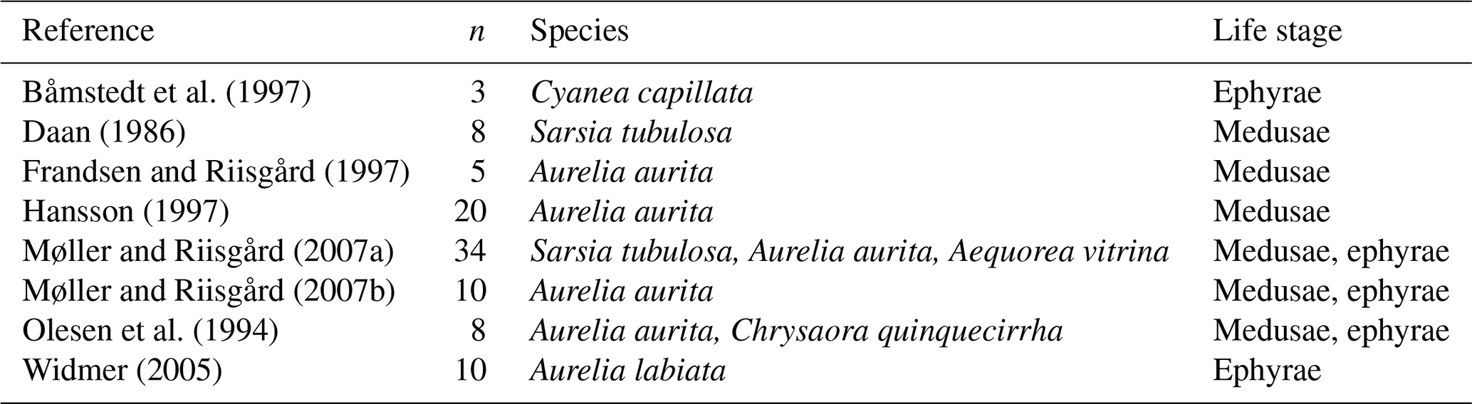
Table A2The fit to the growth data for PFTs for the new three-parameter fit used in this study (see Eq. 3 and Fig. 2) and the two-parameter fit (see Eq. 2 and Fig. 2).

Table A3Sources and metadata for jellyfish grazing preferences, including references with associated species, life stage and preference for prey (categorised into PFTs) with any notable phrases used to inform the grazing of jellyfish in PlankTOM11.
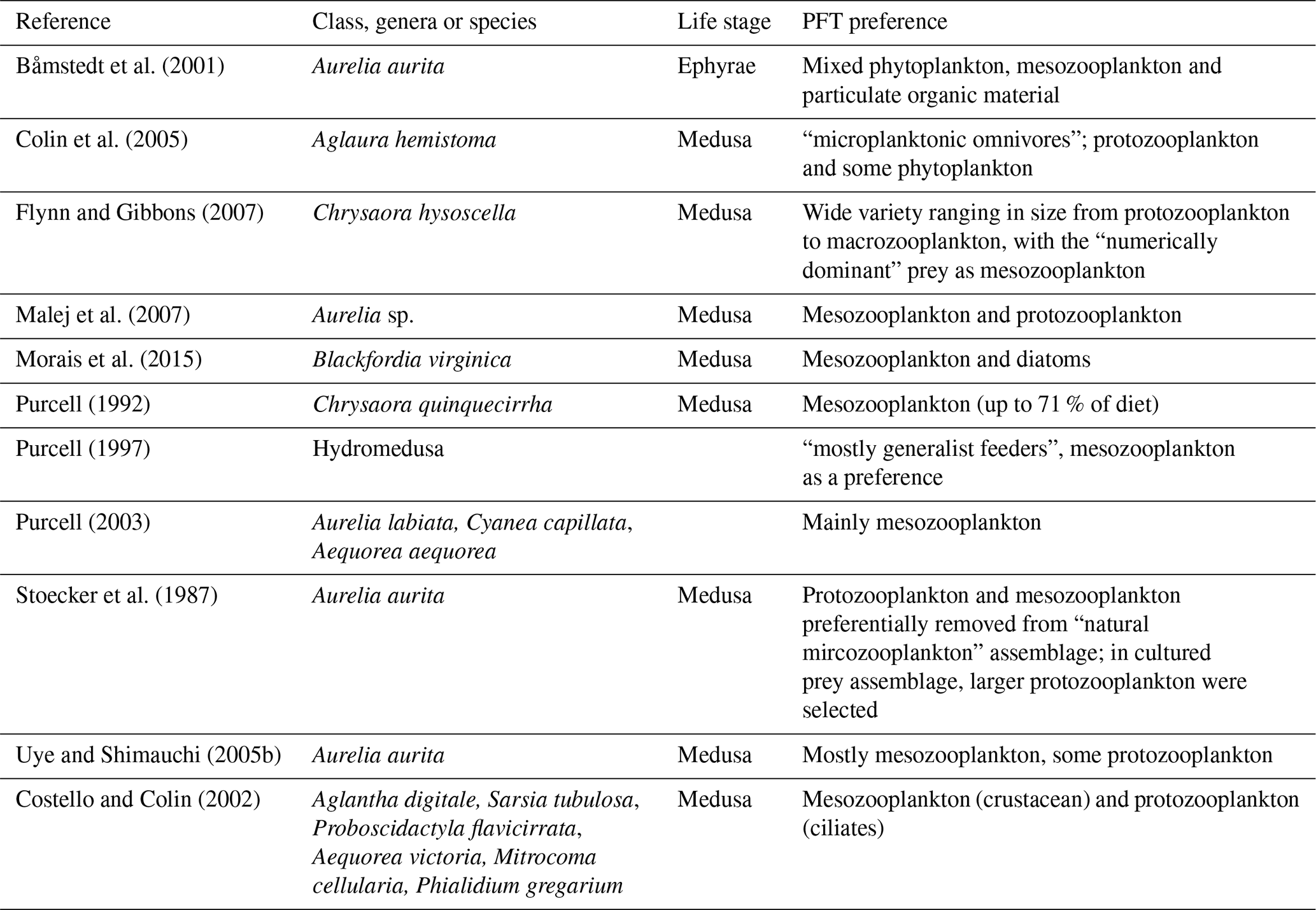
Table A4Additional tuning parameter values for PlankTOM11 (see Sect. 2.1.5) following the change to the growth rate formulation. “Before growth change” values are those used in PlankTOM10LQ16, and “After growth change” values are used in simulations for this study (PlankTOM11, PlankTOM10.5 and PlankTOM10).

Table A5Global mean values for rates and biomass from observations with the associated references. In parenthesis is the percentage share of the plankton type of the total phytoplankton or zooplankton biomass.
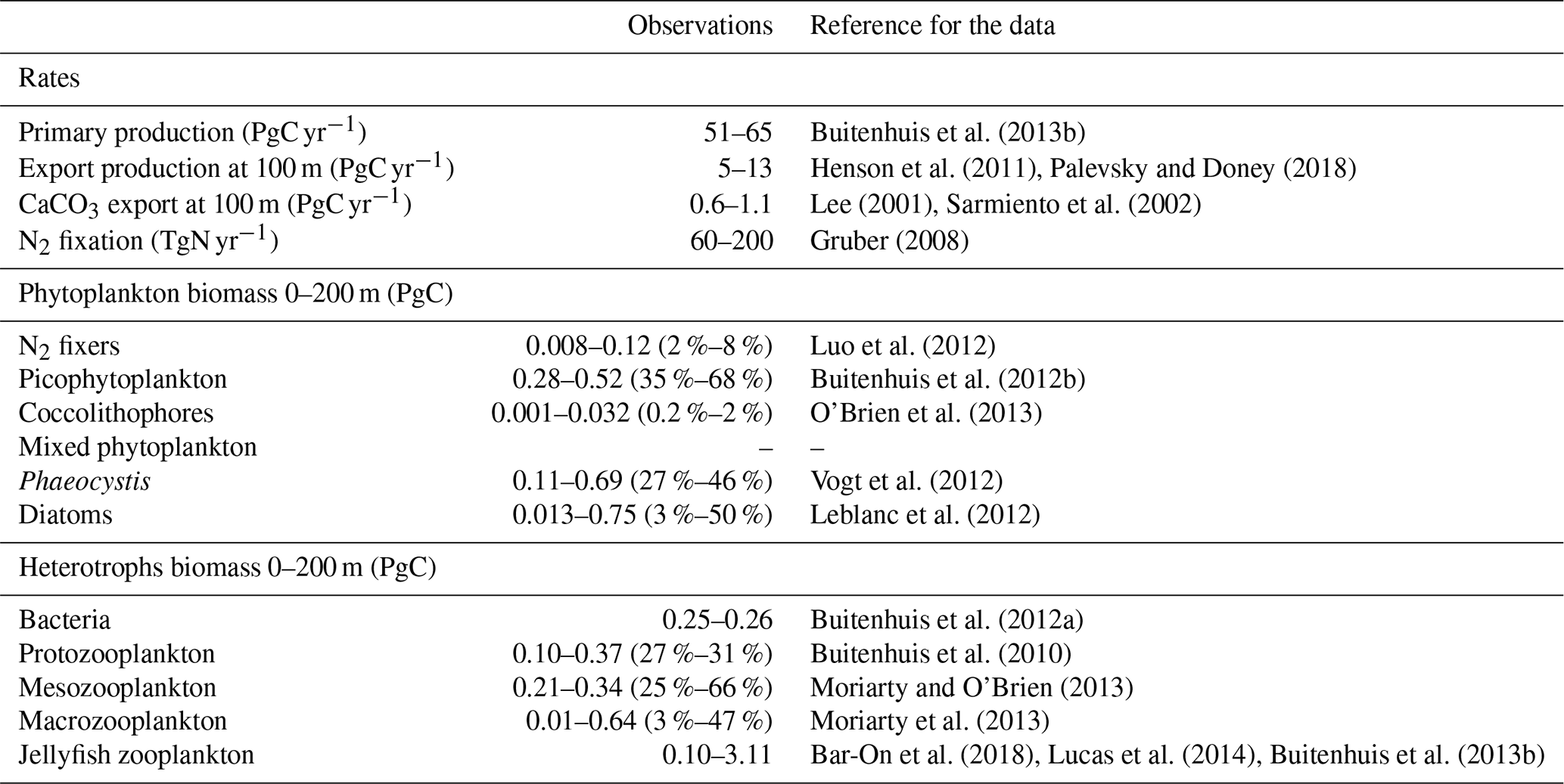
Table A6Total phytoplankton biomass (µmol C L−1) for 30–70∘ N across all longitudes. Observations are from gridded MAREDAT; all data are for the surface ocean (0–10 m). Phytoplankton types include picophytoplankton, Phaeocystis, diatoms, nitrogen fixers and coccolithophores. The seasonal amplitude is the amplitude for the full seasonal cycle (January–December), and the non-winter amplitude is the amplitude for March–October.
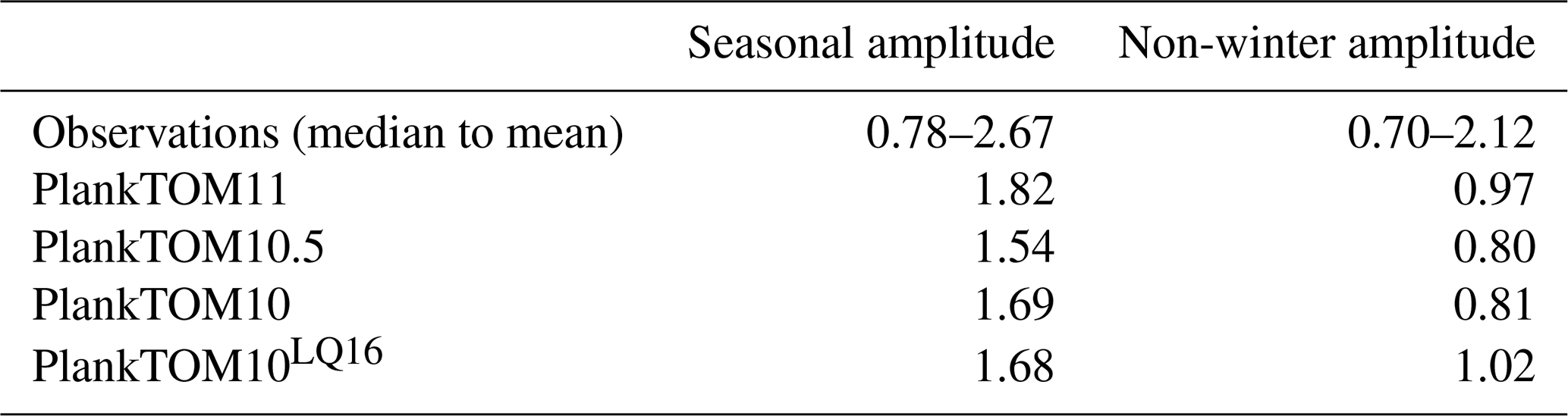

Figure A1Seasonal surface carbon biomass (µmol C L−1) of phytoplankton PFTs; N2 fixers, picophytoplankton, coccolithophores, mixed phytoplankton, Phaeocystis and diatoms. Panels show PFT biomass for PlankTOM11 (a, d), PlankTOM10.5 (b, e) and PlankTOM10 (c, f) for two regions; the north 30–70∘ N (a–c) and the south 30–70∘ S (d–f) across all longitudes. All data are averaged for 1985–2015.
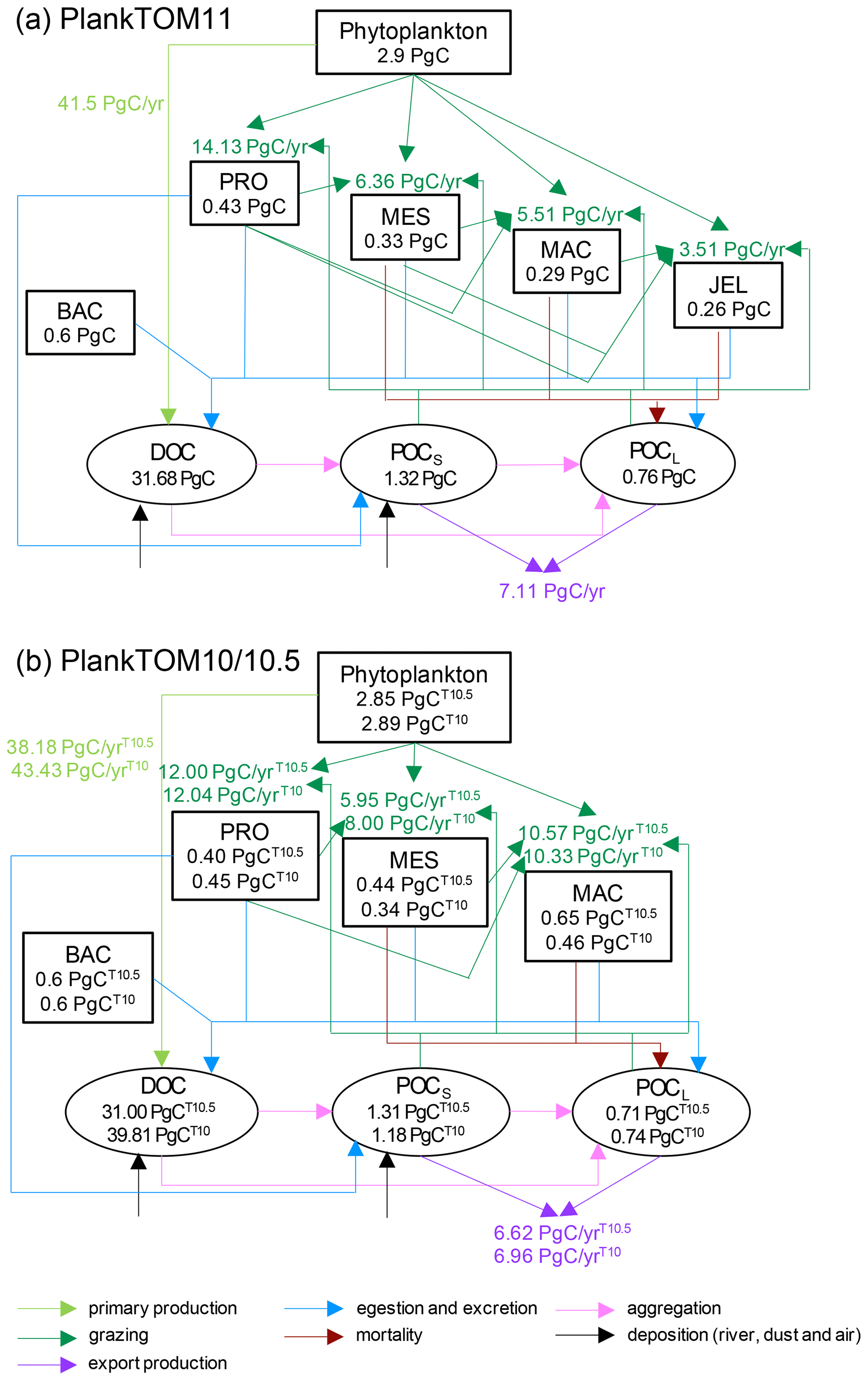
Figure A2Schematic representation of global carbon biomass and rates in the PlankTOM marine ecosystem model including sources and sinks for dissolved organic carbon (DOC) and small (POCS) and large (POCL) particulate organic carbon. (a) PlankTOM11 and (b) PlankTOM10 or PlankTOM10.5. Carbon biomass (PgC) of PFTs and organic carbon pools are given within boxes and ovals respectively. Carbon rates (PgC yr−1) of primary production (light green), grazing (dark green) and export production (purple) are given next to the corresponding arrows. All data are averaged for 1985 to 2015.
The model code can be made available on request by contacting the lead author.
The model data can be made available on request by contacting the lead author.
RMW, CLQ, EB and SP conceptualised the research goals and aims. RMW carried out the formal analysis with contributions from CLQ and EB. RMW developed the model code with significant contributions from EB, and MJG contributed to the development of the jellyfish PFT. RMW performed the simulations. RMW prepared the article with contributions from all co-authors.
The authors declare that they have no conflict of interest.
Rebecca M. Wright was funded by Doctoral Training Programme ARIES, co-funded by the UK Natural Environment Research Council (project no. NE/L002582/1) and CEFAS. Corinne Le Quéré was funded by the Royal Society (grant no. RP\R1\191063). Erik Buitenhuis was funded by the European Commission H2020 project CRESCENDO (grant no. 641816). This research was partly conducted in South Africa with the support of the Newton International PhD exchange programme (grant no. ES/N013948/1). The model simulations were done on the University of East Anglia's High Performance Computing cluster.
This research has been supported by the Natural Environment Research Council (grant no. NE/L002582/1), the Royal Society (grant no. RP\R1\191063), the Newton Fund (grant no. ES/N013948/1), and the European Commission, H2020 European Research Council (CRESCENDO (grant no. 641816)).
This paper was edited by Kenneth Rose and reviewed by two anonymous referees.
Acevedo, M. J., Fuentes, V. L., Olariaga, A., Canepa, A., Belmar, M. B., Bordehore, C., and Calbet, A.: Maintenance, feeding and growth of Carybdea marsupialis (Cnidaria: Cubozoa) in the laboratory, J. Exp. Mar. Bio. Ecol., 439, 84–91, https://doi.org/10.1016/j.jembe.2012.10.007, 2013.
Acuña, J. L., López-Urrutia, Á., and Colin, S.: Faking giants: The evolution of high prey clearance rates in jellyfishes, Science, 333, 1627–1629, https://doi.org/10.1126/science.1205134, 2011.
Almeda, R., Wambaugh, Z., Chai, C., Wang, Z., Liu, Z., and Buskey, E. J.: Effects of crude oil exposure on bioaccumulation of polycyclic aromatic hydrocarbons and survival of adult and larval stages of gelatinous zooplankton, PLoS One, 8, e74476, https://doi.org/10.1371/journal.pone.0074476, 2013.
Antonov, J. I., Seidov, D., Boyer, T., Locarnini, R., Mishonov, A., Garcia, H., Baranova, O., Zweng, M., and Johnson, D.: World Ocean Atlas 2009, US Government Printing Office, Washington, DC, USA, 2010.
Bamstedt, U., Ishii, H., and Martinussen, M. B.: Is the Scyphomedusa Cyanea capillata (L.) dependent on gelatinous prey for its early development?, Sarsia, 83, 269–273, 1997.
Båmstedt, U., Wild, B., and Martinussen, M. B.: Significance of food type for growth of ephyrae Aurelia aurita (Scyphozoa), Mar. Biol., 139, 641–650, https://doi.org/10.1007/s002270100623, 2001.
Bar-On, Y. M., Phillips, R., and Milo, R.: The biomass distribution on Earth, Proc. Natl. Acad. Sci. USA, 115, 6506–6511, https://doi.org/10.1073/pnas.1711842115, 2018.
Benedetti-Cecchi, L., Canepa, A., Fuentes, V., Tamburello, L., Purcell, J. E., Piraino, S., Roberts, J., Boero, F., and Halpin, P.: Deterministic Factors Overwhelm Stochastic Environmental Fluctuations as Drivers of Jellyfish Outbreaks, PLoS One, 10, e0141060, https://doi.org/10.1371/journal.pone.0141060, 2015.
Billett, D. S. M., Bett, B. J., Jacobs, C. L., Rouse, I. P., and Wigham, B. D.: Mass deposition of jellyfish in the deep Arabian Sea, Limnol. Oceanogr., 51, 2077–2083, 2006.
Boero, F., Bucci, C., Colucci, A. M. R., Gravili, C., and Stabili, L.: Obelia (Cnidaria, Hydrozoa, Campanulariidae): A microphagous, filter-feeding medusa, Mar. Ecol., 28, 178–183, https://doi.org/10.1111/j.1439-0485.2007.00164.x, 2007.
Boero, F., Bouillon, J., Gravili, C., Miglietta, M. P., Parsons, T., and Piraino, S.: Gelatinous plankton: irregularities rule the world (sometimes), Mar. Ecol. Prog. Ser., 356, 299–310, https://doi.org/10.3354/meps07368, 2008.
Boero, F., Brotz, L., Gibbons, M. J., Piranio, S., and Zampardi, S.: Impacts and effects of ocean warming on jellyfish, in: Explaining Ocean Warming: Causes, scale, effects and consequences, IUCN, Gland, Switzerland, 213–237, 2016.
Brotz, L., Cheung, W. W. L., Kleisner, K., Pakhomov, E., and Pauly, D.: Increasing jellyfish populations: trends in Large Marine Ecosystems, Hydrobiologia, 690, 3–20, https://doi.org/10.1007/s10750-012-1039-7, 2012.
Buitenhuis, E. T., Le Quéré, C., Aumont, O., Beaugrand, G., Bunker, A., Hirst, A., Ikeda, T., O'Brien, T., Piontkovski, S., and Straile, D.: Biogeochemical fluxes through mesozooplankton, Global Biogeochem. Cy., 20, https://doi.org/10.1029/2005GB002511, 2006.
Buitenhuis, E. T., Rivkin, R. B., Sailley, S., and Le Quéré, C.: Biogeochemical fluxes through microzooplankton, Global Biogeochem. Cy., 24, https://doi.org/doi.org/10.1029/2009GB003601, 2010.
Buitenhuis, E. T., Li, W. K. W., Lomas, M. W., Karl, D. M., Landry, M. R., and Jacquet, S.: Picoheterotroph (Bacteria and Archaea) biomass distribution in the global ocean, Earth Syst. Sci. Data, 4, 101–106, https://doi.org/10.5194/essd-4-101-2012, 2012a.
Buitenhuis, E. T., Li, W. K. W., Vaulot, D., Lomas, M. W., Landry, M. R., Partensky, F., Karl, D. M., Ulloa, O., Campbell, L., Jacquet, S., Lantoine, F., Chavez, F., Macias, D., Gosselin, M., and McManus, G. B.: Picophytoplankton biomass distribution in the global ocean, Earth Syst. Sci. Data, 4, 37–46, https://doi.org/10.5194/essd-4-37-2012, 2012b.
Buitenhuis, E. T., Hashioka, T., and Le Quéré, C.: Combined constraints on global ocean primary production using observations and models, Global Biogeochem. Cy., 27, 847–858, https://doi.org/10.1002/gbc.20074, 2013a.
Buitenhuis, E. T., Vogt, M., Moriarty, R., Bednaršek, N., Doney, S. C., Leblanc, K., Le Quéré, C., Luo, Y.-W., O'Brien, C., O'Brien, T., Peloquin, J., Schiebel, R., and Swan, C.: MAREDAT: towards a world atlas of MARine Ecosystem DATa, Earth Syst. Sci. Data, 5, 227–239, https://doi.org/10.5194/essd-5-227-2013, 2013b.
Chelsky, A., Pitt, K. A., and Welsh, D. T.: Biogeochemical implications of decomposing jellyfish blooms in a changing climate, Estuar. Coast. Shelf Sci., 154, 77–83, https://doi.org/10.1016/j.ecss.2014.12.022, 2015.
Chiaverano, L. M., Robinson, K. L., Tam, J., Ruzicka, J. J., Quiñones, J., Aleksa, K. T., Hernandez, F. J., Brodeur, R. D., Leaf, R., and Uye, S.: Evaluating the role of large jellyfish and forage fishes as energy pathways, and their interplay with fisheries, in the Northern Humboldt Current System, Prog. Oceanogr., 164, 28–36, 2018.
Colin, S. P., Costello, J. H., Graham, W. M., and Higgins III, J.: Omnivory by the small cosmopolitan hydromedusa Aglaura hemistoma, Limnol. Oceanogr., 50, 1264–1268, 2005.
Condon, R. H., Steinberg, D. K., Del Giorgio, P. A., Bouvier, T. C., Bronk, D. A., Graham, W. M., and Ducklow, H. W.: Jellyfish blooms result in a major microbial respiratory sink of carbon in marine systems, Proc. Natl. Acad. Sci. USA, 108, 10225–10230, https://doi.org/10.1073/pnas.1015782108, 2011.
Condon, R. H., Graham, W. M., Duarte, C. M., Pitt, K. A., Lucas, C. H., Haddock, S. H. D., Sutherland, K. R., Robinson, K. L., Dawson, M. N., Beth, M., Decker, M. B., Mills, C. E., Purcell, J. E., Malej, A., Mianzan, H., Uye, S.-I., Gelcich, S., and Madin, L. P.: Questioning the Rise of Gelatinous Zooplankton in the World's Oceans, Bioscience, 62, 160–169, https://doi.org/10.1525/bio.2012.62.2.9, 2012.
Condon, R. H., Duarte, C. M., Pitt, K. A., Robinson, K. L., Lucas, C. H., Sutherland, K. R., Mianzan, H. W., Bogeberg, M., Purcell, J. E., Decker, M. B., Uye, S., Madin, L. P., Brodeur, R. D., Haddock, S. H. D., Malej, A., Parry, G. D., Eriksen, E., Quiñones, J., Acha, M., Harvey, M., Arthur, J. M., and Graham, W. M.: Recurrent jellyfish blooms are a consequence of global oscillations, Proc. Natl. Acad. Sci. USA, 110, 1000–1005, https://doi.org/10.1073/pnas.1210920110, 2013.
Costello, J. H. and Colin, S. P.: Prey resource use by coexistent hydromedusae from Friday Harbor, Washington, Limnol. Oceanogr., 47, 934–942, https://doi.org/10.4319/lo.2002.47.4.0934, 2002.
Crum, K. P., Fuchs, H. L., Bologna, P. A. X., and Gaynor, J. J.: Model-to-data comparisons reveal influence of jellyfish interactions on plankton community dynamics, Mar. Ecol. Prog. Ser., 517, 105–119, https://doi.org/10.3354/meps11022, 2014.
Daan, R.: Food intake and growth of sarsia tubulosa (sars, 1835), with quantitative estimates of predation on copepod populations, Netherlands J. Sea Res., 20, 67–74, 1986.
Doney, S. C., Ruckelshaus, M., Duffy, J. E., Barry, J. P., Chan, F., English, C. A., Galindo, H. M., Grebmeier, J. M., Hollowed, A. B., Knowlton, N., Polovina, J., Rabalais, N. N., Sydeman, W. J., and Talley, L. D.: Climate Change Impacts on Marine Ecosystems, Annu. Rev. Mar. Sci., 4, 11–37, https://doi.org/10.1146/annurev-marine-041911-111611, 2012.
Duarte, C. M., Pitt, K. A., and Lucas, C. H.: Understanding Jellyfish Blooms, in: Jellyfish Blooms, edited by: Pitt, K. A. and Lucas, C. H., Springer, London, UK, 1–5, 2013.
Flynn, B. A. and Gibbons, M. J.: A note on the diet and feeding of Chrysaora hysoscella in Walvis Bay Lagoon, Namibia, during September 2003, African J. Mar. Sci., 29, 303–307, https://doi.org/10.2989/AJMS.2007.29.2.15.197, 2007.
Fossette, S., Gleiss, A. C., Chalumeau, J., Bastian, T., Armstrong, C. D., Vandenabeele, S., Karpytchev, M., and Hays, G. C.: Current-Oriented Swimming by Jellyfish and Its Role in Bloom Maintenance, Curr. Biol., 25, 342–347, https://doi.org/10.1016/j.cub.2014.11.050, 2015.
Frandsen, K. T. and Riisgård, H. U.: Size dependent respiration and growth of jellyfish, Aurelia aurita, Sarsia, 82, 307–312, https://doi.org/10.1080/00364827.1997.10413659, 1997.
Gibbons, M. J. and Richardson, A. J.: Beyond the jellyfish joyride and global oscillations: advancing jellyfish research, J. Plankton Res., 35, 929–938, https://doi.org/10.1093/plankt/fbt063, 2013.
Graham, W. M., Pagès, F., and Hamner, W.: A physical context for gelatinous zooplankton aggregations: a review, Hydrobiologia, 451, 199–212, https://doi.org/10.1023/A:1011876004427, 2001.
Gruber, N.: The Marine Nitrogen Cycle: Overview and Challenges, in Nitrogen in the Marine Environment, 1–50, https://doi.org/10.1016/B978-0-12-372522-6.00001-3, 2008.
Hamner, W. M. and Dawson, M. N.: A review and synthesis on the systematics and evolution of jellyfish blooms: advantageous aggregations and adaptive assemblages, Hydrobiologia, 616, 161–191, https://doi.org/10.1007/s10750-008-9620-9, 2009.
Han, C.-H. and Uye, S.: Combined effects of food supply and temperature on asexual reproduction and somatic growth of polyps of the common jellyfish Aurelia aurita sl, Plankt. Benthos Res., 5, 98–105, 2010.
Hansson, L. J.: Effect of temperature on growth rate of Aurelia aurita (Cnidaria, Scyphozoa) from Gullmarsfjorden, Sweden, Mar. Ecol. Prog. Ser., 161, 145–153, https://doi.org/10.3354/meps161145, 1997.
Hansson, L. J. and Norrman, B.: Release of dissolved organic carbon (DOC) by the scyphozoan jellyfish Aurelia aurita and its potential influence on the production of planktic bacteria, Mar. Biol., 121, 527–532, https://doi.org/10.1007/BF00349462, 1995.
Heneghan, R. F., Everett, J. D., Sykes, P., Batten, S. D., Edwards, M., Takahashi, K., Suthers, I. M., Blanchard, J. L., and Richardson, A. J.: A functional size-spectrum model of the global marine ecosystem that resolves zooplankton composition, Ecol. Modell., 435, 109265, https://doi.org/10.1016/j.ecolmodel.2020.109265, 2020.
Henschke, N., Stock, C. A., and Sarmiento, J. L.: Modeling population dynamics of scyphozoan jellyfish (Aurelia spp.) in the Gulf of Mexico, Mar. Ecol. Prog. Ser., 591, 167–183, https://doi.org/10.3354/meps12255, 2018.
Henson, S. A., Sanders, R., Madsen, E., Morris, P. J., Le Moigne, F., and Quartly, G. D.: A reduced estimate of the strength of the ocean's biological carbon pump, Geophys. Res. Lett., 38, 10–14, https://doi.org/10.1029/2011GL046735, 2011.
Hirst, A. G. and Kiørboe, T.: Mortality of marine planktonic copepods: global rates and patterns, Mar. Ecol. Prog. Ser., 230, 195–209, 2002.
Ikeda, T.: Metabolic rates of epipelagic marine zooplankton as a function of body mass and temperature, Mar. Biol., 85, 1–11, 1985.
Kalnay, E., Kanamitsu, M., Kistler, R., Collins, W., Deaven, D., Gandin, L., Iredell, M., Saha, S., White, G., and Woollen, J.: The NCEP/NCAR 40-year reanalysis project, B. Am. Meteorol. Soc., 77, 437–472, 1996.
Key, R. M., Kozyr, A., Sabine, C. L., Lee, K., Wanninkhof, R., Bullister, J. L., Feely, R. A., Millero, F. J., Mordy, C., and Peng, T.: A global ocean carbon climatology: Results from Global Data Analysis Project (GLODAP), Global Biogeochem. Cy., 18, 1–23, https://doi.org/doi.org/10.1029/2004GB002247, 2004.
Kriest, I. and Oschlies, A.: On the treatment of particulate organic matter sinking in large-scale models of marine biogeochemical cycles, Biogeosciences, 5, 55–72, https://doi.org/10.5194/bg-5-55-2008, 2008.
Lamb, P. D., Hunter, E., Pinnegar, J. K., Creer, S., Davies, R. G., and Taylor, M. I.: Jellyfish on the menu: mtDNA assay reveals scyphozoan predation in the Irish Sea, R. Soc. Open Sci., 4, 171421, https://doi.org/10.1098/rsos.171421, 2017.
Leblanc, K., Arístegui, J., Armand, L., Assmy, P., Beker, B., Bode, A., Breton, E., Cornet, V., Gibson, J., Gosselin, M.-P., Kopczynska, E., Marshall, H., Peloquin, J., Piontkovski, S., Poulton, A. J., Quéguiner, B., Schiebel, R., Shipe, R., Stefels, J., van Leeuwe, M. A., Varela, M., Widdicombe, C., and Yallop, M.: A global diatom database – abundance, biovolume and biomass in the world ocean, Earth Syst. Sci. Data, 4, 149–165, https://doi.org/10.5194/essd-4-149-2012, 2012.
Lebrato, M., Pitt, K. A., Sweetman, A. K., Jones, D. O. B., Cartes, J. E., Oschlies, A., Condon, R. H., Molinero, J. C., Adler, L., Gaillard, C., Lloris, D., and Billett, D. S. M.: Jelly-falls historic and recent observations: a review to drive future research directions, Hydrobiologia, 690, 227–245, https://doi.org/10.1007/s10750-012-1046-8, 2012.
Lebrato, M., Mendes, P. J., Steinberg, D. K., Cartes, J. E., Jones, B. M., Birsa, L. M., Benavides, R., and Oschlies, A.: Jelly biomass sinking speed reveals a fast carbon export mechanism, Limnol. Oceanogr., 58, 1113–1122, 2013a.
Lebrato, M., Molinero, J.-C., Cartes, J. E., Lloris, D., Mélin, F., and Beni-Casadella, L.: Sinking jelly-carbon unveils potential environmental variability along a continental margin, PLoS One, 8, e82070, https://doi.org/10.1371/journal.pone.0082070, 2013b.
Lee, K.: Global net community production estimated from the annual cycle of surface water total dissolved inorganic carbon, Limnol. Oceanogr., 46, 1287–1297, https://doi.org/10.4319/lo.2001.46.6.1287, 2001.
Le Quéré, C., Harrison, S. P., Colin Prentice, I., Buitenhuis, E. T., Aumont, O., Bopp, L., Claustre, H., Cotrim Da Cunha, L., Geider, R., Giraud, X., Klaas, C., Kohfeld, K. E., Legendre, L., Manizza, M., Platt, T., Rivkin, R. B., Sathyendranath, S., Uitz, J., Watson, A. J., and Wolf-Gladrow, D.: Ecosystem dynamics based on plankton functional types for global ocean biogeochemistry models, Glob. Change Biol., 11, 2016–2040, https://doi.org/10.1111/j.1365-2486.2005.1004.x, 2005.
Le Quéré, C., Takahashi, T., Buitenhuis, E. T., Rödenbeck, C., and Sutherland, S. C.: Impact of climate change and variability on the global oceanic sink of CO2, Global Biogeochem. Cy., 24, 1–10, https://doi.org/10.1029/2009GB003599, 2010.
Le Quéré, C., Buitenhuis, E. T., Moriarty, R., Alvain, S., Aumont, O., Bopp, L., Chollet, S., Enright, C., Franklin, D. J., Geider, R. J., Harrison, S. P., Hirst, A. G., Larsen, S., Legendre, L., Platt, T., Prentice, I. C., Rivkin, R. B., Sailley, S., Sathyendranath, S., Stephens, N., Vogt, M., and Vallina, S. M.: Role of zooplankton dynamics for Southern Ocean phytoplankton biomass and global biogeochemical cycles, Biogeosciences, 13, 4111–4133, https://doi.org/10.5194/bg-13-4111-2016, 2016.
Lilley, M. K. S., Beggs, S. E., Doyle, T. K., Hobson, V. J., Stromberg, K. H. P., and Hays, G. C.: Global patterns of epipelagic gelatinous zooplankton biomass, Mar. Biol., 158, 2429–2436, https://doi.org/10.1007/s00227-011-1744-1, 2011.
Lucas, C. H. and Dawson, M. N.: What Are Jellyfishes and Thaliaceans and Why Do They Bloom?, in: Jellyfish blooms, edited by: Pitt K. and Lucas C., Springer, Dordrecht, Springer, 9–44, 2014.
Lucas, C. H., Graham, W. M., and Widmer, C.: Jellyfish Life Histories: role of polyps in forming and maintaining scyphomedusa populations, Adv. Mar. Biol., 63, 133–196, https://doi.org/10.1016/b978-0-12-394282-1.00003-x, 2012.
Lucas, C. H., Jones, D. O. B., Hollyhead, C. J., Condon, R. H., Duarte, C. M., Graham, W. M., Robinson, K. L., Pitt, K. A., Schildhauer, M., and Regetz, J.: Gelatinous zooplankton biomass in the global oceans: geographic variation and environmental drivers, Glob. Ecol. Biogeogr., 23, 701–714, https://doi.org/10.1111/geb.12169, 2014.
Luo, J. Y., Condon, R. H., Stock, C. A., Duarte, C. M., Lucas, C. H., Pitt, K. A., and Cowen, R. K.: Gelatinous Zooplankton-Mediated Carbon Flows in the Global Oceans: A Data-Driven Modeling Study, Global Biogeochem. Cy., 34, e2020GB006704, https://doi.org/10.1029/2020GB006704, 2020.
Luo, Y.-W., Doney, S. C., Anderson, L. A., Benavides, M., Berman-Frank, I., Bode, A., Bonnet, S., Boström, K. H., Böttjer, D., Capone, D. G., Carpenter, E. J., Chen, Y. L., Church, M. J., Dore, J. E., Falcón, L. I., Fernández, A., Foster, R. A., Furuya, K., Gómez, F., Gundersen, K., Hynes, A. M., Karl, D. M., Kitajima, S., Langlois, R. J., LaRoche, J., Letelier, R. M., Marañón, E., McGillicuddy Jr., D. J., Moisander, P. H., Moore, C. M., Mouriño-Carballido, B., Mulholland, M. R., Needoba, J. A., Orcutt, K. M., Poulton, A. J., Rahav, E., Raimbault, P., Rees, A. P., Riemann, L., Shiozaki, T., Subramaniam, A., Tyrrell, T., Turk-Kubo, K. A., Varela, M., Villareal, T. A., Webb, E. A., White, A. E., Wu, J., and Zehr, J. P.: Database of diazotrophs in global ocean: abundance, biomass and nitrogen fixation rates, Earth Syst. Sci. Data, 4, 47–73, https://doi.org/10.5194/essd-4-47-2012, 2012.
Madec, G.: NEMO ocean engine, Note du Pole modeìlisation, Institut Pierre-Simon Laplace, available at: https://zenodo.org/record/1464817 (last access: 2018), 2013.
Malej, A. and Malej, M.: Population dynamics of the jellyfish Pelagia noctiluca (Forsskål, 1775), in: Marine Eutrophication and Populations Dynamics, edited by: Colombo Ferrara, G. I., Olsen & Olsen, Fredensborg, Denmark, 215–219, 1992.
Malej, A., Turk, V., Lučić, D., and Benović, A.: Direct and indirect trophic interactions of Aurelia sp.(Scyphozoa) in a stratified marine environment (Mljet Lakes, Adriatic Sea), Mar. Biol., 151, 827–841, 2007.
Martell, L., Piraino, S., Gravili, C., and Boero, F.: Life cycle, morphology and medusa ontogenesis of Turritopsis dohrnii (Cnidaria: Hydrozoa), Ital. J. Zool., 83, 390–399, https://doi.org/10.1080/11250003.2016.1203034, 2016.
Mills, C. E.: Natural mortality in NR Pacific coastal hydromedusae – grazing predation, wound-healing and senescence, Bull. Mar. Sci., 53, 194–203, 1993.
Møller, L. F. and Riisgård, H. U.: Feeding, bioenergetics and growth in the common jellyfish Aurelia aurita and two hydromedusae, Sarsia tubulosa and Aequorea vitrina, Mar. Ecol. Prog. Ser., 346, 167–177, https://doi.org/10.3354/meps06959, 2007a.
Møller, L. F. and Riisgård, H. U.: Population dynamics, growth and predation impact of the common jellyfish Aurelia aurita and two hydromedusae, Sarsia tubulosa, and Aequorea vitrina in Limfjorden (Denmark), Mar. Ecol. Prog. Ser., 346, 153–165, https://doi.org/10.3354/meps06960, 2007b.
Morais, P., Parra, M. P., Marques, R., Cruz, J., Angélico, M. M., Chainho, P., Costa, J. L., Barbosa, A. B., and Teodósio, M. A.: What are jellyfish really eating to support high ecophysiological condition?, J. Plankton Res., 37, 1036–1041, https://doi.org/10.1093/plankt/fbv044, 2015.
Moriarty, R.: The role of macro-zooplankton in the global carbon cycle, PhD Thesis, University of East Anglia, School of Environmental Sciences, UK, 193 pp., 2009.
Moriarty, R. and O'Brien, T. D.: Distribution of mesozooplankton biomass in the global ocean, Earth Syst. Sci. Data, 5, 45–55, https://doi.org/10.5194/essd-5-45-2013, 2013.
Moriarty, R., Buitenhuis, E. T., Le Quéré, C., and Gosselin, M.-P.: Distribution of known macrozooplankton abundance and biomass in the global ocean, Earth Syst. Sci. Data, 5, 241–257, https://doi.org/10.5194/essd-5-241-2013, 2013.
O'Brien, C. J., Peloquin, J. A., Vogt, M., Heinle, M., Gruber, N., Ajani, P., Andruleit, H., Arístegui, J., Beaufort, L., Estrada, M., Karentz, D., Kopczynska, E., Lee, R., Poulton, A. J., Pritchard, T., and Widdicombe, C.: Global marine plankton functional type biomass distributions: coccolithophores, Earth Syst. Sci. Data, 5, 259–276, https://doi.org/10.5194/essd-5-259-2013, 2013.
Olesen, N. J., Frandsen, K., and Riisgard, H. U.: Population dynamics, growth and energetics of jellyfish Aurelia aurita in a shallow fjord, Mar. Ecol. Prog. Ser., 105, 9–18, https://doi.org/10.3354/meps105009, 1994.
Palevsky, H. I. and Doney, S. C.: How choice of depth horizon influences the estimated spatial patterns and global magnitude of ocean carbon export flux, Geophys. Res. Lett., 45, 4171–4179, 2018.
Pauly, D., Graham, W., Libralato, S., Morissette, L., and Palomares, M. L. D.: Jellyfish in ecosystems, online databases, and ecosystem models, Hydrobiologia, 616, 67–85, https://doi.org/10.1007/s10750-008-9583-x, 2009.
Pitt, K. A., Kingsford, M. J., Rissik, D., and Koop, K.: Jellyfish modify the response of planktonic assemblages to nutrient pulses, Mar. Ecol. Prog. Ser., 351, 1–13, https://doi.org/10.3354/meps07298, 2007.
Pitt, K. A., Welsh, D. T., and Condon, R. H.: Influence of jellyfish blooms on carbon, nitrogen and phosphorus cycling and plankton production, Hydrobiologia, 616, 133–149, 2009.
Pitt, K. A., Budarf, A. C., Browne, J. G., Condon, R. H., Browne, D. G., and Condon, R. H.: Bloom and Bust: Why Do Blooms of Jellyfish Collapse?, in: Jellyfish Blooms, edited by: Pitt, K. A. and Lucas. C. H., Springer, London, UK, 79–103, 2014.
Pitt, K. A., Lucas, C. H., Condon, R. H., Duarte, C. M., and Stewart-Koster, B.: Claims that anthropogenic stressors facilitate jellyfish blooms have been amplified beyond the available evidence: a systematic review, Front. Mar. Sci., 5, 451, https://doi.org/10.3389/fmars.2018.00451, 2018.
Purcell, J. E.: Effects of predation by the Scyphomedusan Chrysaora-quinquecirrha on zooplankton populations in Chesapeake Bay, USA, Mar. Ecol. Prog. Ser., 87, 65–76, https://doi.org/10.3354/meps087065, 1992.
Purcell, J. E.: Pelagic cnidarians and ctenophores as predators: Selective predation, feeding rates, and effects on prey populations, Ann. L Inst. Oceanogr., 73, 125–137, 1997.
Purcell, J. E.: Predation on zooplankton by large jellyfish, Aurelia labiata, Cyanea capillata and Aequorea aequorea, in Prince William Sound, Alaska, Mar. Ecol. Prog. Ser., 246, 137–152, https://doi.org/10.3354/meps246137, 2003.
Purcell, J. E.: Extension of methods for jellyfish and ctenophore trophic ecology to large-scale research, in: Jellyfish Blooms: Causes, Consequences, and Recent Advances, edited by: Pitt, K. and Purcell, J., Springer, Dordrecht, The Netherlands, 23–50, 2009.
Purcell, J. E., Uye, S., and Lo, W.-T.: Anthropogenic causes of jellyfish blooms and their direct consequences for humans: a review, Mar. Ecol. Prog. Ser., 350, 153–174, https://doi.org/10.3354/meps07093, 2007.
Purcell, J. E., Fuentes, V., Atienza, D., Tilves, U., Astorga, D., Kawahara, M., and Hays, G. C.: Use of respiration rates of scyphozoan jellyfish to estimate their effects on the food web, Hydrobiologia, 645, 135–152, 2010.
Ramirez-Romero, E., Molinero, J. C., Paulsen, M., Javidpour, J., Clemmesen, C., and Sommer, U.: Quantifying top-down control and ecological traits of the scyphozoan Aurelia aurita through a dynamic plankton model, J. Plankton Res., 40, 678–692, 2018.
Rhein, M., Rintoul, S. R., Aoki, S., Campos, E., Chambers, D., Feely, R. A., Gulev, S., Johnson, G. C., Josey, S. A., Kostianoy, A., Mauritzen, C., Roemmich, D., Talley, L. D., and Wang, F.: Observations: Ocean, edited by: Stocker, T. F., Qin, D., Plattner, G.-K., Tignor, M., Allen, S. K., Boschung, J., Nauels, A., Xia, Y., Bex, V., and Midgley, P. M., Cambridge University Press, Cambridge, UK New York, NY, USA, 2013.
Richardson, A. J. and Gibbons, M. J.: Are jellyfish increasing in response to ocean acidification?, Limnol. Oceanogr., 53, 2040–2045, 2008.
Rosa, S., Pansera, M., Granata, A., and Guglielmo, L.: Interannual variability, growth, reproduction and feeding of Pelagia noctiluca (Cnidaria: Scyphozoa) in the Straits of Messina (Central Mediterranean Sea): Linkages with temperature and diet, J. Mar. Syst., 111, 97–107, https://doi.org/10.1016/j.jmarsys.2012.10.001, 2013.
Roux, J.-P. and Shannon, L. J.: Ecosystem approach to fisheries management in the northern Benguela: the Namibian experience, African J. Mar. Sci., 26, 79–93, 2004.
Roux, J.-P., van der Lingen, C. D., Gibbons, M. J., Moroff, N. E., Shannon, L. J., Smith, A. D. M., and Cury, P. M.: Jellyfication of marine ecosystems as a likely consequence of overfishing small pelagic fishes: lessons from the Benguela, Bull. Mar. Sci., 89, 249–284, 2013.
Ruzicka, J. J., Brodeur, R. D., Emmett, R. L., Steele, J. H., Zamon, J. E., Morgan, C. A., Thomas, A. C., and Wainwright, T. C.: Interannual variability in the Northern California Current food web structure: Changes in energy flow pathways and the role of forage fish, euphausiids, and jellyfish, Prog. Oceanogr., 102, 19–41, https://doi.org/10.1016/j.pocean.2012.02.002, 2012.
Sarmiento, J. L., Dunne, J., Gnanadesikan, A., Key, R. M., Matsumoto, K., and Slater, R.: A new estimate of the CaCO 3 to organic carbon export ratio, Global Biogeochem. Cy., 16, 1–12, https://doi.org/10.1029/2002gb001919, 2002.
Schnedler-Meyer, N. A., Kiørboe, T., and Mariani, P.: Boom and Bust: Life History, Environmental Noise, and the (un)Predictability of Jellyfish Blooms, Front. Mar. Sci., 5, 257, https://doi.org/10.3389/fmars.2018.00257, 2018.
Schoemann, V., Becquevort, S., Stefels, J., Rousseau, V., and Lancelot, C.: Phaeocystis blooms in the global ocean and their controlling mechanisms: a review, J. Sea Res., 53, 43–66, https://doi.org/10.1016/j.seares.2004.01.008, 2005.
Shannon, L. J., Coll, M., Neira, S., Cury, P., and Roux, J.-P.: Chapter 8: Impacts of fishing and climate change explored using trophic models, in: Climate Change and Small Pelagic Fish, edited by: Checkley, C. R. D. M., Alheit, J., and Oozeki, Y., Cambridge University Press, Cambridge, UK, 158–190, 2009.
Stoecker, D. K., Michaels, A. E., and Davis, L. H.: Grazing by the jellyfish, Aurelia aurita, on microzooplankton, J. Plankton Res., 9, 901–915, https://doi.org/10.1093/plankt/9.5.901, 1987.
Timmermann, R., Goosse, H., Madec, G., Fichefet, T., Ethe, C., and Duliere, V.: On the representation of high latitude processes in the ORCA-LIM global coupled sea ice-ocean model, Ocean Model., 8, 175–201, 2005.
Uye, S. and Shimauchi, H.: Population biomass, feeding, respiration and growth rates, and carbon budget of the scyphomedusa Aurelia aurita in the Inland Sea of Japan, J. Plankton Res., 27, 237–248, https://doi.org/10.1093/plankt/fbh172, 2005a.
Uye, S. and Shimauchi, H.: Population biomass, feeding, respiration and growth rates, and carbon budget of the scyphomedusa Aurelia aurita in the Inland Sea of Japan, J. Plankton Res., 27, 237–248, https://doi.org/10.1093/plankt/fbh172, 2005b.
Vogt, M., O'Brien, C., Peloquin, J., Schoemann, V., Breton, E., Estrada, M., Gibson, J., Karentz, D., Van Leeuwe, M. A., Stefels, J., Widdicombe, C., and Peperzak, L.: Global marine plankton functional type biomass distributions: Phaeocystis spp., Earth Syst. Sci. Data, 4, 107–120, https://doi.org/10.5194/essd-4-107-2012, 2012.
West, E. J., Pitt, K. A., Welsh, D. T., Koop, K., and Rissik, D.: Top-down and bottom-up influences of jellyfish on primary productivity and planktonic assemblages, Limnol. Oceanogr., 54, 2058–2071, https://doi.org/10.4319/lo.2009.54.6.2058, 2009.
Widmer, C. L.: Effects of temperature on growth of north-east Pacific moon jellyfish ephyrae, Aurelia labiata (Cnidaria: Scyphozoa), J. Mar. Biol. Assoc. UK, 85, 569–573, https://doi.org/10.1017/S0025315405011495, 2005.
Yamamoto, J., Hirose, M., Ohtani, T., Sugimoto, K., Hirase, K., Shimamoto, N., Shimura, T., Honda, N., Fujimori, Y., and Mukai, T.: Transportation of organic matter to the sea floor by carrion falls of the giant jellyfish Nemopilema nomurai in the Sea of Japan, Mar. Biol., 153, 311–317, https://doi.org/10.1007/s00227-007-0807-9, 2008.