A climate-dependent global model of ammonia emissions from chicken farming

Ammonia (NH₃) has significant impacts on the environment, which can influence climate and air quality and cause acidification and eutrophication in terrestrial and aquatic ecosystems. Agricultural activities are the main sources of NH₃ emissions globally. Emissions of NH₃ from chicken farming are highly dependent on climate, affecting their environmental footprint and impact. In order to investigate the effects of meteorological factors and to quantify how climate change affects these emissions, a process-based model, AMmonia–CLIMate–Poultry (AMCLIM–Poultry), has been developed to simulate and predict temporal variations in NH₃ emissions from poultry excretion, here focusing on chicken farms and manure spreading. The model simulates the decomposition of uric acid to form total ammoniacal nitrogen, which then partitions into gaseous NH₃ that is released to the atmosphere at an hourly to daily resolution. Ammonia emissions are simulated by calculating nitrogen and moisture budgets within poultry excretion, including a dependence on environmental variables. By applying the model with global data for livestock, agricultural practice and meteorology, we calculate NH₃ emissions from chicken farming on a global scale (0.5^∘ resolution). Based on 2010 data, the AMCLIM–Poultry model estimates NH₃ emissions from global chicken farming of 5.5 ± 1.2 Tg N yr⁻¹, about 13 % of the agriculture-derived NH₃ emissions. Taking account of partial control of the ambient environment for housed chicken (layers and broilers), the fraction of excreted nitrogen emitted as NH₃ is found to be up to 3 times larger in humid tropical locations than in cold or dry locations. For spreading of manure to land, rain becomes a critical driver affecting emissions in addition to temperature, with the emission fraction being up to 5 times larger in the semi-dry tropics than in cold, wet climates. The results highlight the importance of incorporating climate effects into global NH₃ emissions inventories for agricultural sources. The model shows increased emissions under warm and wet conditions, indicating that climate change will tend to increase NH₃ emissions over the coming century.

1 Introduction

Ammonia (NH₃) is the primary form of reactive nitrogen (N_r), which has significant impacts on the environment (Galloway et al., 2003; Sutton et al., 2013). Following its emission to the atmosphere, NH₃ readily reacts with gas-phase acids to form particulate ammonium aerosols and may also condense onto existing particles (Fowler et al., 2009; Hertel et al., 2011). Gaseous NH₃ reacts with sulfuric acid (H₂SO₄) and nitric acid (HNO₃), which leads to the formation of ammonium sulfate ((NH₄)₂SO₄) and ammonium nitrate (NH₄NO₃) aerosols, respectively (Pinder et al., 2007, 2008; Hertel et al., 2011). These particles influence the radiation balance of the Earth, by scattering light and altering the Earth's reflectivity (Xu and Penner, 2012) and also adversely affect regional air quality and human health (Brunekreef and Holgate, 2002; Pinder et al., 2007, 2008). The lifetime of atmospheric NH₃ is relatively short (hours to days), as it is removed rapidly by dry and wet deposition or converted to ammonium aerosols (Hendriks et al., 2016). Consequently, it is usually removed close to its source. In terrestrial ecosystems, acute exposure to NH₃ can cause visible foliar injury, reducing the vegetation's tolerance to pests and diseases, especially for native plants and forests (Krupa, 2003; Stulen et al., 1998; Sutton et al., 2011). Once deposited in water, NH₃ can result in acidification and eutrophication (Sutton et al., 2011). Excess N_r input causes algal blooms in vulnerable aquatic ecosystems, which harms local biodiversity.

The dominant source of NH₃ emission is from agricultural activities, including animal housing, manure storage and fertilizer usage for arable lands and crops. In Western countries, approximately 80 %–90 % of atmospheric releases are from agriculture (Sutton et al., 2000; Hertel et al., 2011); a major source of NH₃ emission is from livestock waste. Oenema et al. (2007) estimated that NH₃ emissions cause a loss of approximately 19 % of nitrogen from livestock housing and manure storage, with a further 19 % being lost following the land application of manure. Previous studies that quantified NH₃ emissions from livestock have made estimations mainly by empirical methods. Emission factors were used, assuming fixed values for nitrogen volatilization rates, varying by animal type and management practices. For example, Misselbrook et al. (2000) derived NH₃ emission factors for major animals under various farming practices in UK agriculture. The advantage of this method is the relative simplicity for calculations. However, these emission factors only include climatic effects to a small extent. Using a fixed number to describe the fraction of excreted nitrogen that volatilizes as NH₃ does not always provide a realistic value under all environmental conditions and may cause large uncertainties in large-scale estimations (e.g. when considering global-scale estimates). Sommer and Hutchings (2001) reviewed a range of empirical models that were produced to predict NH₃ volatilization from slurry application to land. These models have experiment-derived equations. However, only the effect of temperature and slurry dry matter content were studied, and the interactions between these parameters were not investigated.

Another method for estimating NH₃ emissions from livestock is to use process-based models based on a theoretical understanding of relevant processes, building on foundations developed for field sources (Sutton et al., 1995b; Nemitz et al., 2001; Móring et al., 2016). Pinder et al. (2004) developed a process-based model for simulating NH₃ emissions from dairy cows, and the modelled NH₃ volatilization fraction from grazing, manure spreading and storage was shown to be reasonable compared to independent experimental data. Previous process-modelling efforts for bird sources have focused on native seabird populations (Riddick et al., 2016, 2018), using these as a natural laboratory to study the effect of global climate differences on NH₃ emissions, supported by a programme of measurements through different climates (Blackall et al., 2007; Riddick et al. 2012). Process-based models consider the effects of meteorological variation on the formation of NH₃ from an N_r source, allowing the calculation of NH₃ emissions that vary temporally and spatially. They can be extended to investigate the influences of various environmental conditions. However, as more complicated parameterizations are included in process-based models, more detailed inputs are required, and a lack of input data may limit the model's ability to obtain better results.

Ammonia emissions from animal waste are understood to be highly climate sensitive. For example, Sutton et al. (2013) showed a factor of 9 increase in emission rates between 5 and 25 ^∘C, with additional effects from humidity and precipitation (Riddick et al., 2017). Poultry numbers have increased roughly five-fold over the last 50 years (FAO, 2018), with chickens being the largest fraction. Global usage of poultry manure for land spreading increased from an estimated 5.0 Tg N yr⁻¹ in 2000 to 6.3 Tg N yr⁻¹ in 2010 (FAO, 2018). However, limited research has attempted to determine the magnitude of global NH₃ emissions from chicken farming whilst also considering climatic effects. In this study, a process-based model, AMmonia–CLIMate–Poultry (AMCLIM–Poultry), has been developed to simulate and predict temporal variations in NH₃ emissions from three major chicken production systems, namely (a) broilers, (b) layers and (c) backyard chicken, focusing on chicken housing and land spreading of manure. The overarching goals of this study are to develop a process-based model and to apply it at global scale, to produce improved NH₃ emission estimates under the influences of various meteorological factors and to estimate total NH₃ emissions and their distribution for the present-day (year 2010) for chicken farming globally. Future work will quantify the estimated response of NH₃ emissions to climate change, the potential for year-to-year variability and the implications for NH₃ emissions from other livestock sectors.

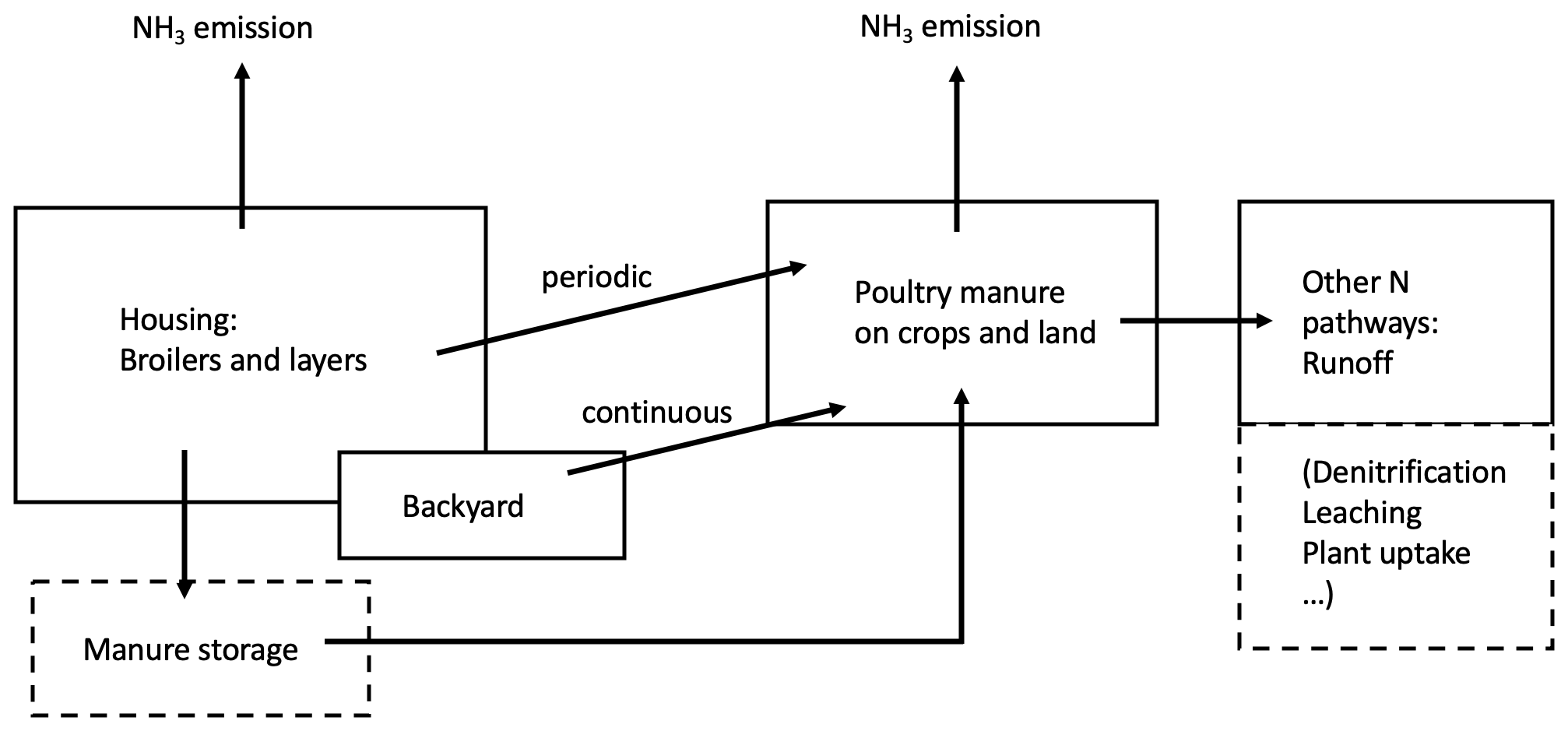
Figure 1 Schematic of the AMCLIM–Poultry model for estimating NH₃ emissions from global chicken farming, following nitrogen pathways from chicken farms to land spreading. Arrows represent the nitrogen flows from chicken farming. Aspects noted in dashed boxes are not investigated in this study.

2 Methods and materials

2.1 Model description

Figure 1 shows the agricultural activities in which chicken litter is a source of NH₃ emission. Nitrogenous manure can be used as fertilizers on land or be stored for future use. Typically, litter collected from chicken houses is spread on arable lands at the start of planting period, while excretions from backyard systems are applied fresh to fields or left on pastures and other ground. Ammonia can be released to the atmosphere through each of these activities. In this study, we developed the process-based AMCLIM–Poultry model to quantify NH₃ emissions from chicken farming, focusing on housing and manure land spreading. For this purpose, it is assumed in the model that emissions from stored manure occur within the animal house (in-house storage) or do not behave significantly differently.

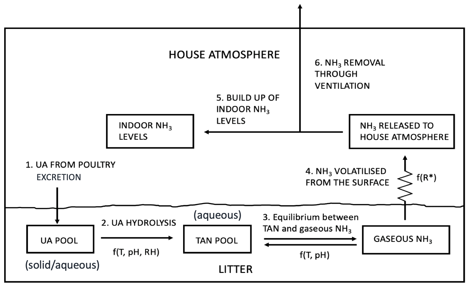
Figure 2 Schematic of NH₃ volatilization in the poultry house. UA is uric acid; TAN is total ammoniacal nitrogen; R^∗ is the resistance for gaseous transfer from the litter surface to the in-house atmosphere (adapted from Elliott and Collins, 1982).

The model has been developed from the GUANO model (Riddick et al., 2017) that simulates NH₃ emissions from wild seabird colonies, which provides a starting point for AMCLIM–Poultry. Both models simulate N_r through the decomposition processes that uric acid (UA; solid/aqueous phase) in excreta hydrolyses to form total ammoniacal nitrogen (TAN = NH₃ + NH${}_{\mathrm{4}}^{+}$; aqueous phase), which then partitions to form gaseous NH₃ that is released to the atmosphere (Fig. 2). Major advances in the present study, using AMCLIM–Poultry compared with the GUANO model, include the following:

• There is a distinction between indoor and outdoor simulations, which represent different practices and production systems under different environmental conditions (housing birds, manure spreading and backyard birds).

• The flow of nitrogen is conserved between the different stages of housing and manure spreading following excretion, which reflects the reality that nitrogen emitted as NH₃ cannot be emitted again.

• A new approach is developed to simulate indoor emissions. Environmental conditions of houses and a new parameterization for UA hydrolysis are generalized from measurement data sets. Ammonia volatilized from the animal waste at the surface is determined by a parameterized resistance term that is derived from measurements.

• The land spreading of chicken manure is linked to the timing of agricultural cropping cycles, which allows a better estimate of NH₃ emissions and its temporal variations.

We used chicken excretal nitrogen as an input (described in Sect. 2.4.1) and incorporated meteorological factors to predict temporal variations in the NH₃ emissions. The quantitative equations used in the model are described below using SI units. The model was operated with an hourly time step for outdoor simulations and a daily time step for indoor simulations.

2.1.1 Mass balance of nitrogen components

The AMCLIM–Poultry model simulates masses for N-containing components (UA and TAN) within the chicken farming system (chicken houses, backyard chickens and chicken manure spreading) and flows between these pools (Fig. 1). The mass per unit area of excretion (M_excretion, g m⁻²; all model variables are described, with units, in the Appendix) over the time step Δt is calculated following Eq. (1):

$$\begin{array}{}\text{(1)}& M_{\text{excretion}}\left(t+\mathrm{\Delta }t\right)=M_{\text{excretion}}\left(t\right)+{\displaystyle \frac{F_{\text{e}}}{f_{\text{N}}}}\mathrm{\Delta }t,\end{array}$$

where F_e (all nitrogen flows have units of g N m⁻² s⁻¹) is the total nitrogen excretion rate from chicken, and f_N (g N g excretion⁻¹) is the nitrogen content of excretion. The evolution of UA mass (M_UA; all nitrogen pool masses have units of g N m⁻²) is calculated following Eq. (2):

$$\begin{array}{}\text{(2)}& M_{\text{UA}}\left(t+\mathrm{\Delta }t\right)=M_{\text{UA}}\left(t\right)+(F_{\text{e}}{f}_{\text{UA}}-F_{\text{TAN}})\mathrm{\Delta }t,\end{array}$$

where f_UA is the UA fraction in the excretion, and F_TAN is the flux of TAN that is decomposed from UA hydrolysis.

Similarly, the mass of TAN (M_TAN) is calculated following Eq. (3):

$$\begin{array}{}\text{(3)}& M_{\text{TAN}}\left(t+\mathrm{\Delta }t\right)=M_{\text{TAN}}\left(t\right)+(F_{\text{TAN}}-F_{{\text{NH}}_{\mathrm{3}}})\mathrm{\Delta }t,\end{array}$$

where $F_{{\mathrm{NH}}_{\mathrm{3}}}$ is the net rate of conversion of TAN to gaseous NH₃ that is emitted to the atmosphere. All pools are set to zero when there is an emptying event for housing.

2.1.2 Process-based simulation of nitrogen pathways

For each emission context (i.e. animal housing, backyard birds and manure spreading), the AMCLIM–Poultry model includes three key steps, namely conversion of UA to TAN, equilibrium between aqueous phase TAN and gaseous NH₃ in the litter, and volatilization of NH₃ from the litter surface to the atmosphere (Fig. 2). The hydrolysis of UA to TAN is strongly affected by temperature, the pH of the substrate and the relative humidity (RH) of the chicken house atmosphere (Elliott and Collins, 1982; Elzing and Monteny, 1997; Koerkamp, 1994). The production rate of TAN is determined from the UA mass and the conversion rate (K), which is a function of these three factors as follows:

$$\begin{array}{}\text{(4)}& F_{\text{TAN}}=M_{\text{UA}}{K}_{(T,\text{pH},\text{RH})}.\end{array}$$

The maximum estimated production rate is 20 % d⁻¹ at 35 ^∘C, pH 9.0 and RH 80 % (Elliot and Collins, 1982). The combined influence of these three factors is the product of a series of conversion rate functions, as follows:

$$\begin{array}{}\text{(5)}& K_{(T,\text{pH},\text{RH})}=\mathrm{0.2}{k}_{\text{pH}}{k}_T{k}_{\text{RH}}.\end{array}$$

Gas phase NH₃, held within the litter pore spaces, is in equilibrium with TAN that depends upon the litter pH and temperature response of combined Henry and disassociation equilibria (Eq. 6; Nemitz et al., 2000). The gas phase concentration of NH₃ in air (χ) at the surface is proportional to the aqueous phase ratio Γ = [${\mathrm{NH}}_{\mathrm{4}}^{+}]/[{\mathrm{H}}^{+}]$ of the chicken litter, which is calculated from Eqs. (6) and (7) as follows:

$$\begin{array}{}\text{(6)}& {\displaystyle }\mathit{\chi }={\displaystyle \frac{\mathrm{161}\mathrm{500}}{T}}\exp \left({\displaystyle \frac{-\mathrm{10}\mathrm{378}}{T}}\right)\mathrm{\Gamma },\text{(7)}& {\displaystyle }\mathrm{\Gamma }={\displaystyle \frac{\left[{\text{NH}}_{\mathrm{4}}^{+}\right]}{\left[{\mathrm{H}}^{+}\right]}}={\displaystyle \frac{\left[\text{TAN}\right]}{K_{{\text{NH}}_{\mathrm{4}}^{+}}+\left[{\mathrm{H}}^{+}\right]}}={\displaystyle \frac{M_{\text{TAN}}}{V_{{\mathrm{H}}_{\mathrm{2}}\mathrm{O}}\left(K_{{\text{NH}}_{\mathrm{4}}^{+}}+\left[{\mathrm{H}}^{+}\right]\right)}},\end{array}$$

where $V_{{\mathrm{H}}_{\mathrm{2}}\mathrm{O}}$ (mL m⁻²) is the volume of water in the litter, and $K_{{\mathrm{NH}}_{\mathrm{4}}^{+}}$ is the dissociation constant of NH${}_{\mathrm{4}}^{+}$. Ammonia volatilizes to the atmosphere from the surface at a rate ($F_{{\mathrm{NH}}_{\mathrm{3}}}$) that can be determined by assuming a resistance type model, i.e. using gas concentrations at two vertical levels constrained by a set of resistances (Sutton et al., 2013), which is calculated from Eq. (6) as follows:

$$\begin{array}{}\text{(8)}& F_{{\mathrm{NH}}_{\mathrm{3}}}={\displaystyle \frac{\left[\mathit{\chi }\right(z_{\text{o'}})-\mathit{\chi }(z\left)\right]}{\left[R_{\text{a}}\right(z)+R_{\text{b}}]}},\end{array}$$

where χ(z_o') represents the concentration at the surface, and χ(z) represents the concentration at a reference height. Equation (7) is the general formula. For an in-house application of the model, χ(z) is taken as representative of well-mixed indoor concentrations of NH₃ in the chicken house. For an outdoor application of the model, the reference height is taken 10 m above ground. R_a and R_b are the aerodynamic and boundary layer resistances, respectively. This broad resistance approach is applicable for manure spread in the field and is also applied for backyard birds. For resistance in the chicken houses, a modified approach is needed, as described in Sect. 2.2.2.

2.2 Simulations for chicken housing

Figure 2 illustrates the process pathways through which NH₃ volatilizes from the N-rich chicken excretion to the exterior atmosphere. We assumed that 60 % of excreted nitrogen is in the form of UA (f_UA=0.6), which accounts for approximately 3 %–8 % of the chicken excretion (Nahm, 2003). The remaining 40 % of excreted nitrogen is assumed to be from other forms that do not lead to significant NH₃ emissions. Uric acid accumulates in the litter of the chicken house until it converts to TAN by bacterial ammonification, with TAN concentrations in equilibrium with the litter pore space concentration of gaseous NH₃. Ammonia is then emitted from the surface, which builds up the indoor NH₃ levels within the house through mixing. Meanwhile, as the indoor NH₃ must be controlled below a certain level, ventilation continuously removes NH₃ and brings fresh air, which dilutes the NH₃ concentrations.

We used the monitored data from animal feeding operations (AFOs, 2012) to simulate site-specific NH₃ emissions from chicken houses. The data were gathered by the US Environmental Protection Agency (EPA) as a study of emissions from different types of livestock from 2007 to 2010 (Cortus et al., 2010; Jin-Qin Ni et al., 2010; Wang et al., 2010). As shown in Table S1 (Supplement Sect. S1), two broiler houses and four layer houses from three US farms at different sites were selected for this study. We used daily mean animal data, environmental data and indoor NH₃ concentrations (measured at 2–2.5 m above the ground; representative of well-mixed air in the chicken house) from these sites. Animal data included bird numbers, body weight and biomaterial data for each house. Environmental data included temperature, relative humidity for natural (outdoor) and indoor conditions and the interior ventilation given as an airflow rate in m³ s⁻¹. We filled up missing environmental data to keep simulations continuous by using a linear interpolation method when measurements were unavailable. Excreted nitrogen was determined from the animal data and was used as an input to the model, together with the indoor environmental data. As the AMCLIM–Poultry model does not simulate evaporation from litter in houses, we determined the excretion water content ($M_{{\mathrm{H}}_{\mathrm{2}}\mathrm{O}}\left(\text{e}\right)$; g m⁻²) based on the equilibrium moisture content (m_E; %) of the litter, which is calculated from Eq. (7) as follows:

$$\begin{array}{}\text{(9)}& M_{{\mathrm{H}}_{\mathrm{2}}\mathrm{O}}\left(\text{e}\right)={\displaystyle \frac{m_{\text{E}}}{\mathrm{100}}}\cdot M_{\text{excretion}},\end{array}$$

where m_E is calculated following the Eq. (8):

$$\begin{array}{}\text{(10)}& m_{\text{E}}={\left[{\displaystyle \frac{-\ln (\mathrm{1}-\frac{\text{RH}}{\mathrm{100}})}{\mathrm{0.0000534}\times T}}\right]}^{\frac{\mathrm{1}}{\mathrm{1.41}}},\end{array}$$

where RH (in percent) is the relative humidity, and T (K) is the temperature (Elliott and Collins, 1982). Equation (10) is based on the hygroscopicity of chicken litter and accounts for the moisture absorbed by the litter as it reaches an equilibrium state, which is dependent on temperature and RH.

2.2.1 Parameterization of UA hydrolysis rate for chicken housing

The hydrolysis of UA to TAN plays a crucial role in affecting NH₃ emissions. The rate of conversion of UA to TAN is often the rate-limiting process that determines the overall rate of conversion of nitrogen excreted by chickens into NH₃ emissions. The parameterization of UA to TAN conversion is therefore very important for the overall model performance.

In the study of Elliott and Collins (1982), a chicken litter model was used to investigate the UA hydrolysis rate. They set the base level conversion rate to 20 % over a 24 h period under optimal conditions (pH = 9; T≥35 ^∘C; RH ≥ 80 %), and then produced empirical functions to account for the influence of these three factors. In order to evaluate the validity of these empirical functions, specifically temperature and RH effects, we analysed the AFO measurements for two layer houses from the US EPA data set (Table S1), starting from the date that the litter was cleaned out from the houses. We assumed an equilibrium state between the production of TAN and NH₃ emissions. It should be noted that the equilibrium state does not always apply, but it is a useful assumption for parameterization, and the introduced uncertainty is discussed in Sect. 4.1.1. The temperature dependence was derived from measurements when RH was over 80 %, and the RH dependence was derived from measurements that were normalized by the temperature dependence.

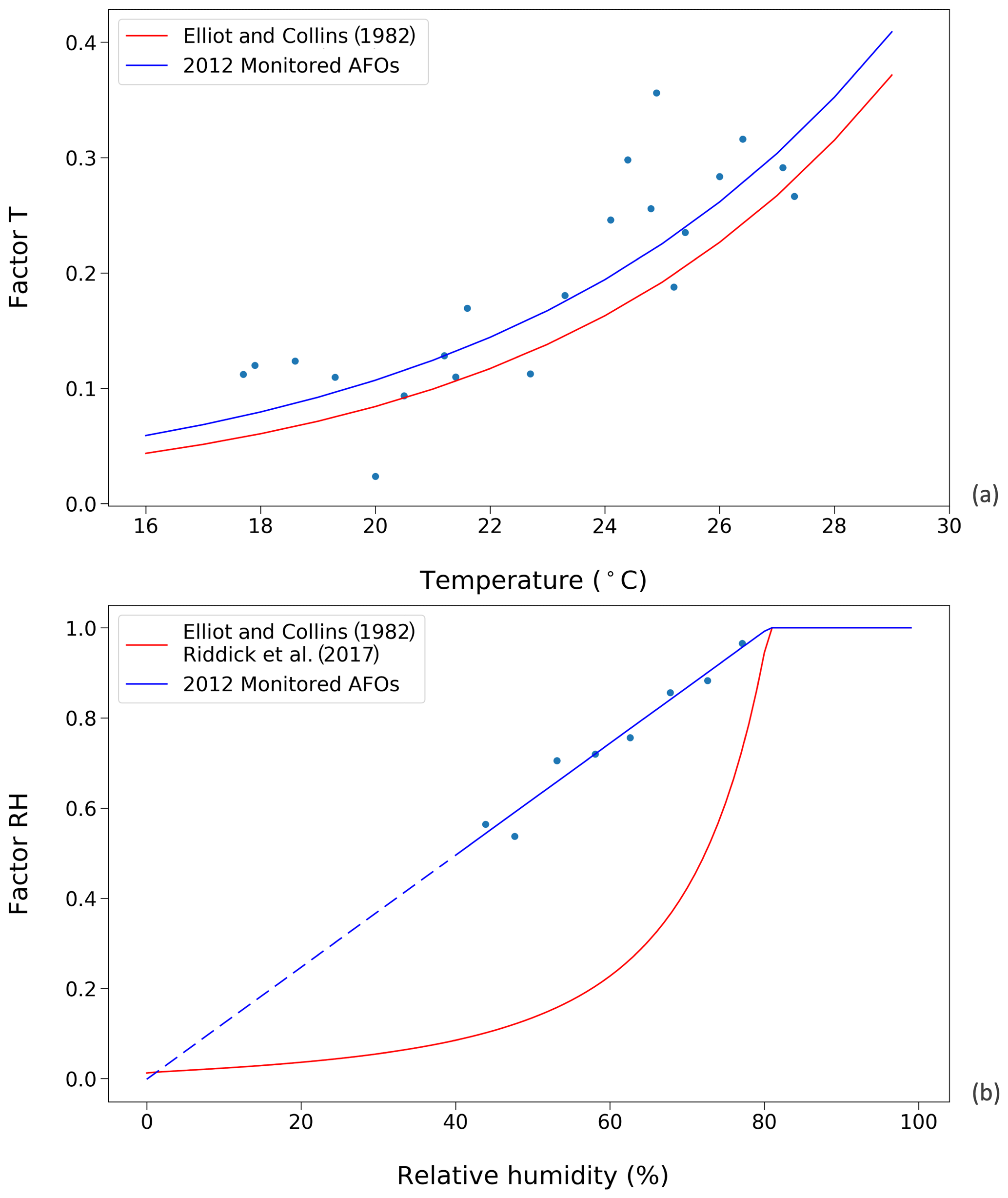
Figure 3 Factors affecting UA hydrolysis rate in chicken houses. Red curves represent the results from Elliott and Collins (1982). Blue curves represent results from this study, using data from the 2012 monitored animal feeding operations (AFOs; see Sect. 2.2.1). (a) Influence of temperature on UA hydrolysis. (b) Influence of relative humidity (RH) on UA hydrolysis at optimum temperature condition (≥35 ^∘C). The dashed line is the extrapolation of factor RH as a function of RH due to a lack of data when relative humidity was below 40 % in the AFO experiments.

The temperature and RH dependence of the UA hydrolysis rate derived from using the AFO-monitored data are shown in Fig. 3, where they are compared to functions from Elliott and Collins (1982). The new temperature dependence follows an exponential relationship and is normalized to the maximum rate at 35 ^∘C as follows:

$$\begin{array}{}\text{(11)}& k_T={\displaystyle \frac{{\text{exp}}^{(\mathrm{0.149}\left(T-\mathrm{273.15}\right)+\mathrm{0.49})}}{{\text{exp}}^{(\mathrm{0.149}\left(\mathrm{35}\right)+\mathrm{0.49})}}}.\end{array}$$

The new RH dependence increases linearly as RH increases, reaching the maximum rate of one at RH 80 % as follows:

$$\begin{array}{}\text{(12)}& k_{\text{RH}}=\left\{\begin{array}{l}\mathrm{0.0125}\text{RH}-\mathrm{0.0014},\text{if}\mathrm{0}<\text{RH}<\mathrm{80}\mathit{\%}\\ \mathrm{1},\text{if}\text{RH}\mathrm{80}\mathit{\%}\le \text{RH}.\end{array}\right.\end{array}$$

Within the range of RH 0 %–40 %, the function is extrapolated due to the limited data at these conditions (Fig. 3b). The new RH dependence is parameterized directly as a function of RH rather than the excretion moisture content because it is envisaged that fresh excretion reaches an moisture equilibrium within a few hours, and it is a representative simplification to use the RH data as the model is run on a daily time step.

We used the pH dependence for the range of 5.5 to 9.0 from the Elliott and Collins (1982) study as follows:

$$\begin{array}{}\text{(13)}& k_{\text{pH}}={\displaystyle \frac{\mathrm{1.34}\left(\text{pH}\right)-\mathrm{7.2}}{\mathrm{1.34}\left(\mathrm{9}\right)-\mathrm{7.2}}}.\end{array}$$

A fixed pH of 8.5 that is the typical value of poultry manure (Elliott and Collins, 1982; Sommer and Hutchings, 2001) was used for the simulations. We did not include a dynamical scheme for determining pH influenced by the UA hydrolysis (see Móring et al., 2016), which is a practicable simplification for a global model.

2.2.2 Inversion of resistance within chicken houses to develop R^∗ parameterization of chicken houses

The NH₃ flux from an unvegetated surface to the atmosphere is mainly constrained by two terms, namely aerodynamic resistance (R_a) and boundary layer resistance (R_b; Wesely, 1989). Outdoors, both of these resistances are related to meteorological conditions and can be calculated. However, values of R_a and R_b within chicken houses remain unknown due to the lack of knowledge of turbulence for indoor conditions. We estimated the overall indoor resistance, termed R^∗, which includes R_a, R_b and also the resistance of litter, by inverting the measured AFO data. As shown by steps 4, 5 and 6 in Fig. 2, the interior NH₃ level within a chicken house is determined by the source flux from the litter surface and the removal flux through ventilation. Mathematically, the total flux of NH₃ (F_surface; g N s⁻¹) from the surface is expressed as Eq. (12) in the following:

$$\begin{array}{}\text{(14)}& F_{\text{surface}}=\left({\displaystyle \frac{{\mathit{\chi }}_{\text{surface}}-{\mathit{\chi }}_{\text{in}}}{R^{\ast }}}\right)\cdot S,\end{array}$$

where χ_surface (g m⁻³) is the in-house value of χ(z_o'), i.e. the gaseous NH₃ concentration at the litter surface, and χ_in (g m⁻³) is the indoor NH₃ concentration of the house, assuming a complete mixing of air inside the chicken house. R^∗ (s m⁻¹) is the indoor resistance, and S (m²) is the surface area of the house. The NH₃ removal (F_removal; g N s⁻¹) through ventilation is expressed as Eq. (13) in the following:

$$\begin{array}{}\text{(15)}& F_{\text{removal}}=Q({\mathit{\chi }}_{\text{in}}-{\mathit{\chi }}_{\text{out}}),\end{array}$$

where χ_out (g m⁻³) is the free-atmosphere NH₃ concentration. χ_out is set to be 0.3 µg m⁻³, which is normally much lower than the indoor concentration. Q (m³ s⁻¹) represents the ventilation rate. Therefore, by mass conservation, we can relate indoor NH₃ concentrations and the interior air volume V (m³) to surface emissions and losses through ventilation as follows:

$$\begin{array}{}\text{(16)}& \begin{array}{rl}& V{\displaystyle \frac{\mathrm{d}{\mathit{\chi }}_{\text{in}}}{\mathrm{d}t}}=F_{\text{surface}}-F_{\text{removal}}\\ & =\left({\displaystyle \frac{{\mathit{\chi }}_{\text{surface}}-{\mathit{\chi }}_{\text{in}}}{R^{\ast }}}\right)\cdot S-Q\left({\mathit{\chi }}_{\text{in}}-{\mathit{\chi }}_{\text{out}}\right).\end{array}\end{array}$$

For inversion of R^∗, we used the data for two layer houses at NC2B, which had clearly reported house-emptying dates and had fewer missing measurement data. The simulation period started from the day when the litter was cleaned out, and each nitrogen pool was re-initialized. We assumed the house reached a steady state (hence the left-hand side of Eq. (10) is zero) after a period of simulation for 3 d, and the term Qχ_out has been neglected due to its small magnitude. Subsequently, the resistance can be calculated from Eq. (15) as follows:

$$\begin{array}{}\text{(17)}& R^{\ast }={\displaystyle \frac{({\mathit{\chi }}_{\text{surface}}-{\mathit{\chi }}_{\text{in}})\cdot S}{Q{\mathit{\chi }}_{\text{in}}}}.\end{array}$$

To develop this parameterization, the gas phase NH₃ concentration at the surface (χ_surface) was simulated by the AMCLIM–Poultry model, and the NH₃ concentration within the house and ventilation were taken from the AFO-monitored data.

2.3 Simulations of NH₃ emission from chicken manure spreading

Simulations for the spreading of chicken manure on fields followed the processes of nitrogen pathways, which are similar to the housing simulations. Nevertheless, there are several key points that need to be clarified. First, contrary to housing, the amount of water is calculated in a different way, relative to the environmental conditions, which includes rainfall, evaporation and run-off rather than only depending on litter moisture. Second, run-off takes place during rain events and is a major loss of nitrogen. Third, aerodynamic resistance (R_a) and boundary layer resistance (R_b) that determine the magnitude of NH₃ emissions are directly calculated from meteorological variables instead of being parameterized (Nemitz et al., 2001; Seinfeld and Pandis, 2016; Riddick et al., 2017). Details are given in Sect. S2. Fourth, we only simulate processes taking place in manure and do not simulate interactions with soils. We consider it reasonable, as chicken manure is mainly applied on the land surface because it is dry and not physically mixed with underlying soils based on the assumption of a simple application scenario. In addition, simulating soil processes would require a much more detailed characterization of soil chemistry, which might only be achieved by using sophisticated land models that are beyond the scope of this study.

The amount of water in the litter ($M_{{\mathrm{H}}_{\mathrm{2}}\mathrm{O}}$, g m⁻²) is calculated from the following:

$$\begin{array}{}\text{(18)}& \begin{array}{rl}& M_{{\mathrm{H}}_{\mathrm{2}}\mathrm{O}}\left(t+\mathrm{\Delta }t\right)=\\ & \left\{\begin{array}{l}{M}_{{\mathrm{H}}_{\mathrm{2}}\mathrm{O}}\left(t\right)-M_{\text{available\hspace{0.17em} water}}+\left(F_{{\mathrm{H}}_{\mathrm{2}}\mathrm{O}}\left(\text{rain}\right)-F_{{\mathrm{H}}_{\mathrm{2}}\mathrm{O}}\left(\text{evap}\right)\right)\mathrm{\Delta }t\\ +M_{{\mathrm{H}}_{\mathrm{2}}\mathrm{O}}\left(\text{e}\right),\text{if}\\ M_{{\mathrm{H}}_{\mathrm{2}}\mathrm{O}}\left(t\right)-M_{\text{available\hspace{0.17em} water}}+\left(F_{{\mathrm{H}}_{\mathrm{2}}\mathrm{O}}\left(\text{rain}\right)-F_{{\mathrm{H}}_{\mathrm{2}}\mathrm{O}}\left(\text{evap}\right)\right)\mathrm{\Delta }t>\mathrm{0}\\ M_{{\mathrm{H}}_{\mathrm{2}}\mathrm{O}}\left(\text{e}\right),\text{if}\\ M_{{\mathrm{H}}_{\mathrm{2}}\mathrm{O}}\left(t\right)-M_{\text{available\hspace{0.17em} water}}+\left(F_{{\mathrm{H}}_{\mathrm{2}}\mathrm{O}}\left(\text{rain}\right)-F_{{\mathrm{H}}_{\mathrm{2}}\mathrm{O}}\left(\text{evap}\right)\right)\mathrm{\Delta }t\le \mathrm{0},\end{array}\right.,\end{array}\end{array}$$

where $F_{{\mathrm{H}}_{\mathrm{2}}\mathrm{O}}\left(\text{rain}\right)$ (g m⁻² s⁻¹) and $F_{{\mathrm{H}}_{\mathrm{2}}\mathrm{O}}\left(\text{evap}\right)$ (g m⁻² s⁻¹) are the rainfall and evaporation, respectively, and M_{available  water} (g m⁻² s⁻¹) is the water available for run-off. It should be noted that the amount of water in the manure should not be less than the excretion water content, which is the equilibrium moisture content dependent on environmental conditions.

In the model, the immediate run-off (M_N-runoff; g m⁻²) is derived from a run-off coefficient multiplied by the nitrogen pools as follows:

$$\begin{array}{}\text{(19)}& M_{\text{N-runoff}}=R_{\text{runoff}}\cdot M_{\text{N}},\end{array}$$

where the M_N (g m⁻²) is the amount of each N-containing components, and R_runoff is the run-off coefficient that is a function of the amount of water within the nitrogen pools available for run-off (Q_{available  water}; millimetres) as follows:

$$\begin{array}{}\text{(20)}& R_{\text{runoff}}=Q_{\text{available\hspace{0.17em} water}}\cdot r_{\text{N}},\end{array}$$

where r_N (mm⁻¹) represents the wash-off factor, and constant values of 1 % per millimetre and 0.5 % per millimetre were used for nitrogen and manure, respectively (Riddick et al., 2017). The amount of water available for run-off (M_{available  water}, g m⁻²) is determined by subtracting the water absorbed by the manure from rainfall as follows:

$$\begin{array}{}\text{(21)}& M_{\text{available\hspace{0.17em} water}}=F_{{\mathrm{H}}_{\mathrm{2}}\mathrm{O}}\left(\text{rain}\right)\mathrm{\Delta }t-\mathrm{2}\times M_{\text{excretion}}.\end{array}$$

The maximum amount of water that can be absorbed by the manure was assumed to be 2 times the mass of excretion (Riddick et al., 2017).

2.4 Global applications

2.4.1 Model input

We applied the AMCLIM–Poultry model at the global scale to quantify the NH₃ emissions from global chicken farming. The model used the Food and Agricultural Organization of the United Nations (FAO) global chicken density data and chicken excretion nitrogen data as input and was driven by the European Centre for Medium-Range Weather Forecasts (ECMWF) ERA5 hourly meteorological data (ERA5, 2018). The model was run at a resolution of $\mathrm{0.5}{}^{\circ }\times \mathrm{0.5}{}^{\circ }$, with the global chicken density data and nitrogen data being regridded to fit the 0.5^∘ resolution.

The global population of chickens was based on the Food and Agriculture Organization Corporate Statistical Database (FAOSTAT) data for 2010. The geographic distribution was based on the Gridded Livestock of the World (GLW) model, which produced density maps for the main livestock species based on observed densities and explanatory variables such as climatic data, land cover and demographic parameters (Robinson et al., 2014). The chicken data were categorized into three production systems, namely broilers, layers and backyard chicken. Broilers and layers are major chicken types that are reared intensively in buildings and managed by farmers or livestock companies. The environment for rearing backyard chicken is varied, and the density is lower compared to broilers or layers. The distinction in the global distribution of backyard and intensive systems was based on Gilbert et al. (2015). Birds in the intensive systems were further subdivided into broilers and layers, using the procedure developed for the Global Livestock Environmental Assessment Model (GLEAM; FAO, 2018a). The GLEAM approach was also used to produce the nitrogen excretion maps, which were calculated as the difference between nitrogen intake and retention. The total nitrogen intake depends on feed intake and nitrogen content of the feed, while the retention is the amount of nitrogen that is retained in birds' tissues, either as live weight gain or the production of eggs (FAO, 2018b).

2.4.2 Global upscaling for chicken housing

In chicken farms, the inside conditions can be distinct from the natural environment. The lower critical temperature for chicken (i.e. the minimum managed temperature for optimum chicken performance) is approximately 16–20 ^∘C (Gyldenkærne et al., 2005), which is much higher than of other livestock, such as cattle and sheep. Intensively managed chicken are typically kept in insulated buildings with forced ventilation and heating systems to help maintain fixed temperature throughout the year as far as feasible (Seedorf et al., 1998). To keep the ambient temperature within a recommended range, the house may be heated or ventilated in relation to outdoor temperatures. Heating occurs on cold days when the temperature is low but not in other periods. Ventilation is to maintain a healthy condition for chickens' growth, and a minimum level is required, but the ventilation should also be below a certain rate to avoid an induced draft in the house (Gyldenkærne et al., 2005).

For the modelling, the broilers and layers were assumed to be kept in buildings with adequate heating and ventilation systems. The density for broilers and layers was assumed to be 15 and 30 birds per square metre, respectively (Cortus et al., 2010; Jin-Qin Ni et al., 2010; Krause and Schrader, 2019; Wang et al., 2010). The environmental parameters incorporated in the model are empirically derived from the indoor environment of chicken farms reported in the EPA data set. The housing temperature is determined by the generalized relationships between indoor and outdoor or natural temperatures, as shown in Fig. S1 (Sect. S3 in the Supplement), while the RH in the house is set to be identical to ambient RH as no obvious relationship was found according to the EPA data set. It is assumed that the temperature and ventilation rates of chicken houses are maintained as close as possible to a stable level throughout the day and are driven by the natural climatic conditions under local practice. There is no precipitable water in the house, so the water pool excludes precipitation and is purely related to the excretion moisture. The litter in chicken houses was assumed to be removed once a year. The housing simulation of the AMCLIM–Poultry model was operated at a daily time step for 2010, as the indoor conditions are derived from daily measurements. To calculate the varying impacts of emptying the chicken houses at different times of the year, we ran 12 different year-long simulations, each starting from a different month, i.e. from January to December, and assuming that the chicken house had just been emptied. The results were averaged and reported in this study.

2.4.3 Global upscaling for chicken manure spreading

As shown in Fig. 1, manure from chicken farms is collected for spreading on fields, leading to NH₃ emissions. Typically, fertilizing crops use manure from local farms. Therefore, we assumed the amount of nitrogen from chicken manure is only spread locally, and the simulations for each grid cell are independent of the adjacent ones in terms of model input. This assumption is considered to be valid at a $\mathrm{0.5}{}^{\circ }\times \mathrm{0.5}{}^{\circ }$ resolution of the global model application (equivalent to 39 km × 55 km at 45^∘ latitude), though it cannot be automatically assumed when modelling at finer scales. The available nitrogen budgets were determined from the amount of nitrogen left, ensuring mass consistency to account for NH₃ emitted in the housing simulations.

It should be emphasized that the land spreading of chicken manure must only take place in regions that have arable lands, and the amount of nitrogen applied on the land should not exceed the total manure N application rates. To address these considerations, we compared the available amount of chicken manure N (nitrogen left in manure after being lost as NH₃ at housing period) to the total amount of manure N for crops to identify places that use chicken manure as fertilizer. Data of the total amount of manure N used for crops and fertilizing areas were taken from West et al. (2014). We chose six major crops for which chicken manure is an ideal fertilizer, including barley, maize, potato, rice, sugar beet and wheat. We assumed that the chicken manure is primarily applied to these six crops. For areas where available chicken manure N does not exceed the total manure N application, we calculated the nitrogen input for individual crops with Eq. (20) as follows:

$$\begin{array}{}\text{(22)}& N_{\text{Crop\_Poultry}}=N_{\text{Available}}\cdot {\displaystyle \frac{N_{\text{Crop}}}{N_{\text{Total\_Manure}}}}.\end{array}$$

Conversely, for areas where available nitrogen input from chicken exceeds the total manure N application, the nitrogen input is calculated from Eq. (21) as follows:

$$\begin{array}{}\text{(23)}& N_{\text{Crop\_Poultry}}=N_{\text{Crop}},\end{array}$$

where N_{Crop_Poultry} (g N m⁻²) is the amount of chicken manure N application for individual crops, N_Available (g N m⁻²) is the amount of available chicken manure N, N_Crop (g N m⁻²) is the amount of total nitrogen application for individual crops, and N_{Total_Manure} (g N m⁻²) is the amount of total nitrogen application from manure for all crops. The excess nitrogen in these areas was considered to be applied to other crops. In regions where annual nitrogen applications are zero, we assumed the available chicken manure N are untreated and left on land.

Planting and harvesting dates for crops are important parameters in the model because they determine the meteorological conditions of the crop-growing period, which affects the temporal variations in NH₃ emissions from land spreading. Fertilizer applied to land or crops is dependent on the timing of agricultural activities rather than being spread frequently. As a result, the NH₃ emissions from fertilizer spreading usually shows strong seasonal variations due to the local farming practice. The AMCLIM–Poultry model incorporates the planting and harvesting dates from the Crop Calendar Dataset for the six major crops (Sacks et al., 2010). We developed a relatively simple scenario for manure applications in which the chicken manure was applied at the start of the planting period. The timing of agricultural practices in the Southern Hemisphere is different from the Northern Hemisphere. The planting activities usually start in November or December, which means that partial NH₃ emissions in these regions would occur in the next year. Similarly, manure spreading that took place in the previous year can also result in emissions in the current year. Therefore, we ran the model for more than 1 year to keep an annual cycle of simulation period for each grid. It should be emphasized that our model scenario assumes a standard reference that all chicken manure is broadcast on the surface of bare agricultural fields at the start of the cropping cycle. Other future scenarios could consider the effectiveness of management practices in mitigating NH₃ emissions from the spreading of chicken manure (see Sect. 4.5).

As introduced in Sect. 2.4.1, backyard chickens are one of the major production systems included in the FAO chicken density data set. In comparison with broilers and layers, backyard chickens are reared in residential lots rather than in insulated houses. According to the FAO statistics, there are two general ways of dealing with excretion from backyard chickens, namely daily spreading and leaving it on pastures. Consequently, the simulations for NH₃ emissions from backyard chickens were set to be under natural environments. Data for excreted nitrogen from backyard chickens from the FAO data set were used as the nitrogen input to the model. The density was assumed to be four birds per square metre. The meteorological inputs were the same as those used in the simulations for chicken manure spreading for crops. The model was operated at an hourly time step for a period of 1 year as an initialization. The second-year simulation was for the study period of 2010.

3 Results

3.1 Site simulations for chicken housing

3.1.1 Temperature of chicken houses

A generalized representation of the indoor temperatures of chicken housing was empirically derived from the AFO measurements from the three farms. The relationships between indoor temperature and outdoor temperature of broiler houses and layer houses are different (Fig. S1). In layer houses, temperature is considered to be primarily dependent to the outdoor temperature, while broiler houses' temperature is also related to broilers' body weights. The data for when broilers' body weight is less than 0.5 kg per bird are excluded from the parameterization because (a) broilers that are smaller than this size do not contribute significantly to NH₃ emissions, and (b) houses are kept warmer than normal for the smallest chicks compared to birds heavier than 0.5 kg. By excluding these data for small birds, a much better relationship can be found between indoor and outdoor temperatures (Fig. S1), which is also representative of the periods of significant NH₃ emissions. In running the AMCLIM–Poultry model for global upscaling, the same relationship from Fig. S1 is applied for all weights of birds, including layers and broilers.

Figure 4 Site simulations using a fixed resistance (R^∗) value of 16 700 s m⁻¹ for House A at site NC2B, Nash, North Carolina, from 15 March 2008 to 15 March 2009. (a) Measured daily mean indoor temperature and airflow rate of the house. (b) Measured daily mean relative humidity of the house. (c) Modelled TAN pool and UA pool. The black dashed line indicates the house-emptying date of 9 April 2008. (d) Comparison between measured and modelled indoor NH₃ concentrations of the house and surface NH₃ concentrations. (e) Comparison between modelled NH₃ emissions and calculated NH₃ emissions from measured indoor concentrations. The simulation illustrated uses the new parameterization (based on the AFO data; Fig. 3) for the relative humidity dependence of UA hydrolysis.

3.1.2 Resistance within chicken houses and site simulations

The inversion-derived resistance within chicken houses, R^∗, is presented in Figs. S2 to S5 (Sect. S4); strong daily variations can be seen. The possible relationships of calculated R^∗ values to temperature and ventilation rate were investigated. This showed no strong correlation with these indoor environmental variables (See Figs. S6 and S7). We simulated the total NH₃ emissions with various constant R^∗ values throughout the year and compare the results to the measurements (Fig. S8). A fixed R^∗ value of ∼ 16 700 s m⁻¹ was found to provide the best result of 1:1 for House A and ∼ 14 369 s m⁻¹ for House B at NC2B.

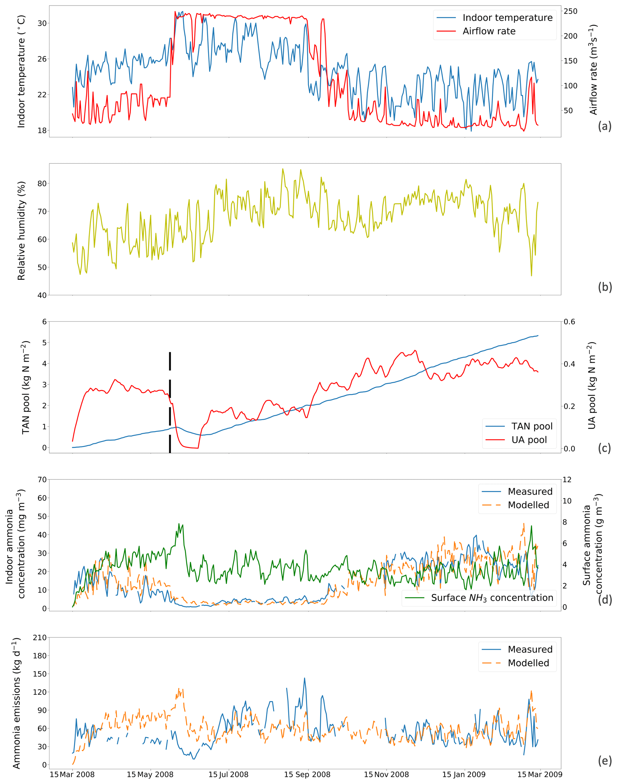
Figure 5 The same as Fig. 4 but for simulations using a fixed resistance (R^∗) value of 14 369 s m⁻¹ for House B at site NC2B, Nash, North Carolina, from 15 March 2008 to 15 March 2009. The black dashed line indicates the house-emptying date of 3 June 2008.

Figures 4 and 5 show the simulated indoor NH₃ concentrations and emissions compared to the measurements by assuming the fixed R^∗ value of 167 00 and 14 369 s m⁻¹, respectively. Gaps shown in measured concentrations and emissions of NH₃ represent unavailable measurements, while the model was kept running during gaps to produce a continuous output. The model was able to capture the major changes throughout the simulation period. During hot periods of the year, the temperature inside the house was generally higher than the cold months, and ventilation rates reached the maximum. High temperature led to large UA hydrolysis that increased the TAN pool, which allows more NH₃ emissions. High ventilation rates accelerated the NH₃ removal from the house, and the indoor concentration of NH₃ decreased. The TAN pool of both houses accumulated and reached approximately 5 kg per square metre, while the UA pools were relatively low due to the continuous conversion to TAN. Sharp declines in the UA pools were seen (9 April 2008 in House A; 3 June 2008 in House B), linked to the chicken houses being empty at these times (as shown by black dashed lines) for approximately 3 weeks. The NH₃ concentrations at the surface were much higher than the NH₃ concentrations of the house atmospheres in both houses. As a result, with sufficient TAN and large differences between surface and air NH₃ concentration, NH₃ emissions in the summer months were higher than in winter months. The model overestimated NH₃ emissions from early April to early July and then underestimated the emissions in September for House B. The discrepancies are mainly caused by the use of a fixed housing resistance, R^∗. In reality, R^∗ will vary with the environmental conditions within chicken houses. However, we consider it well justified to use a constant value of R^∗ in order to keep the overall fit of the data set to the measured emissions simple, which also simplifies the global application.

3.1.3 Model sensitivity to temperature and relative humidity

To understand the effects of temperature and relative humidity on the NH₃ volatilization in chicken houses, we ran simulations under idealized conditions. We used a configuration (i.e. animal number and house size), the same as the NC2B House A, but set the temperature and relative humidity to constant values throughout the whole year. A spin-up year run was done prior to the experimental simulations.

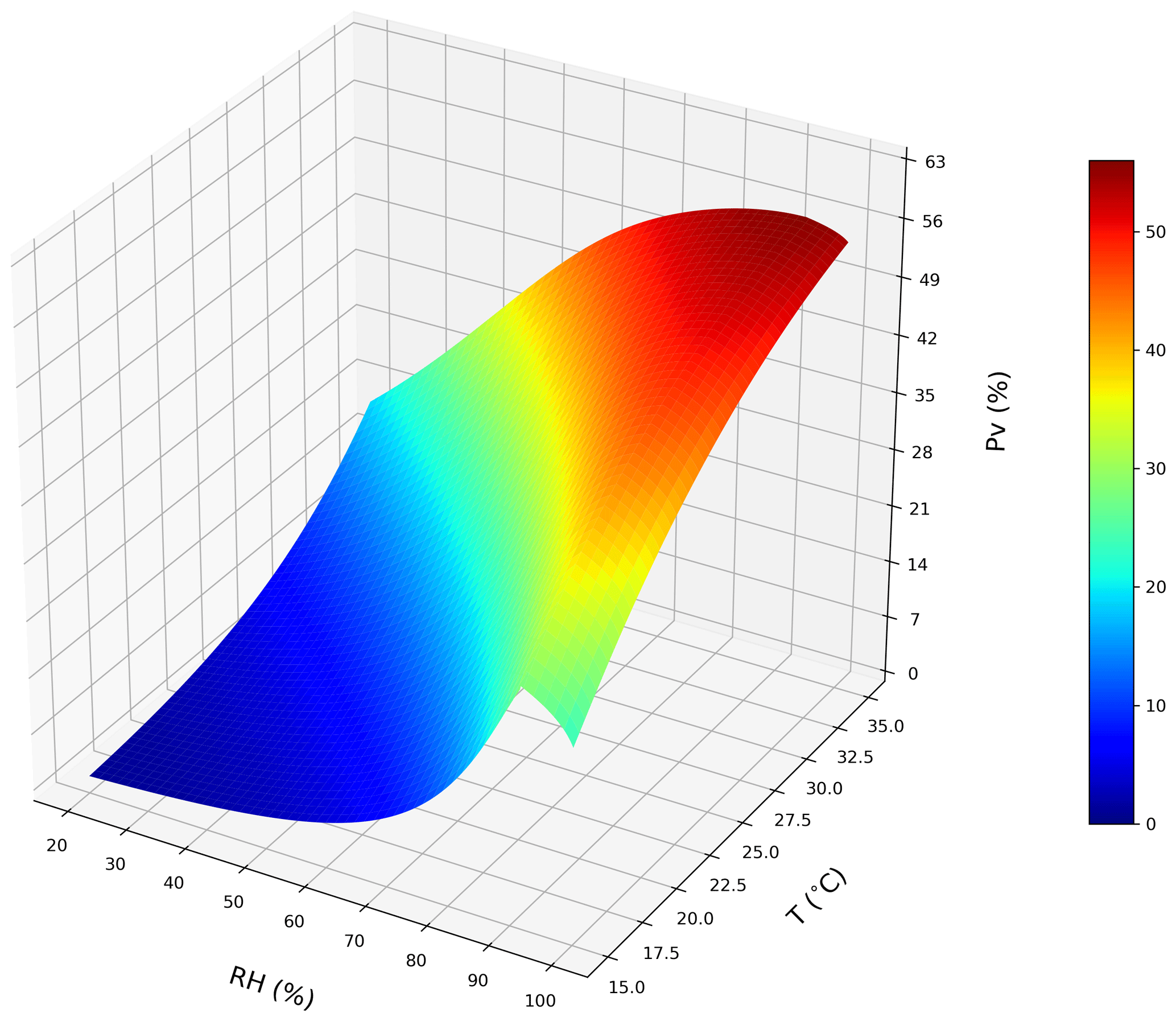
Figure 6 A conceptual 3D sketch of the NH₃ volatilization rate (P_V) that is driven by temperature (T) and relative humidity (RH). The surface plot is derived from a set of idealized steady-state simulations with zero precipitation to simulate dependences for emissions from chicken housing (see Sect. 2.2.1; shown using the new parameterizations for T and RH).

We tested the NH₃ volatilization rate (P_V) under a domain with temperature range of 15–35 ^∘C and RH range of 20 %–100 %. Figure 6 shows an overall increase in P_V from a low temperature and RH to a high temperature and RH regime. The highest P_V values reaching approximately 56 % were from high temperature and RH simulations. Figure 7a shows that the P_V rates increase as temperature increases, and Fig. 7b also shows that the P_V rates increase as RH increases but drop after RH exceeds 90 %.

Figure 7 Curves that represent NH₃ volatilization rate (P_V) for four different temperature and RH regimes based on annual idealized simulations (see Fig. 6). (a) The NH₃ volatilization rate (P_V) under dry (20 % RH) and wet (100 % RH) conditions, respectively. (b) The NH₃ volatilization rate (P_V) under 15 and 35 ^∘C, respectively. (See Sect. 2.2.1; shown using the new parameterizations for temperature and RH).

3.2 Site simulations for land spreading

We ran a set of simple site experiments for land spreading to quantify the NH₃ volatilization under different environmental conditions. The model configurations of these simulations are given in detail in the Supplement Sect. S5. We compare the model results with reported measurements from five experimental studies (Lau et al., 2008; Marshall et al., 1998; Miola et al., 2014; Rodhe and Karlsson, 2002; Sharpe et al., 2004). There are three groups of comparisons that represent different simulation and measurement duration at 7, 14 and 21 d, respectively.

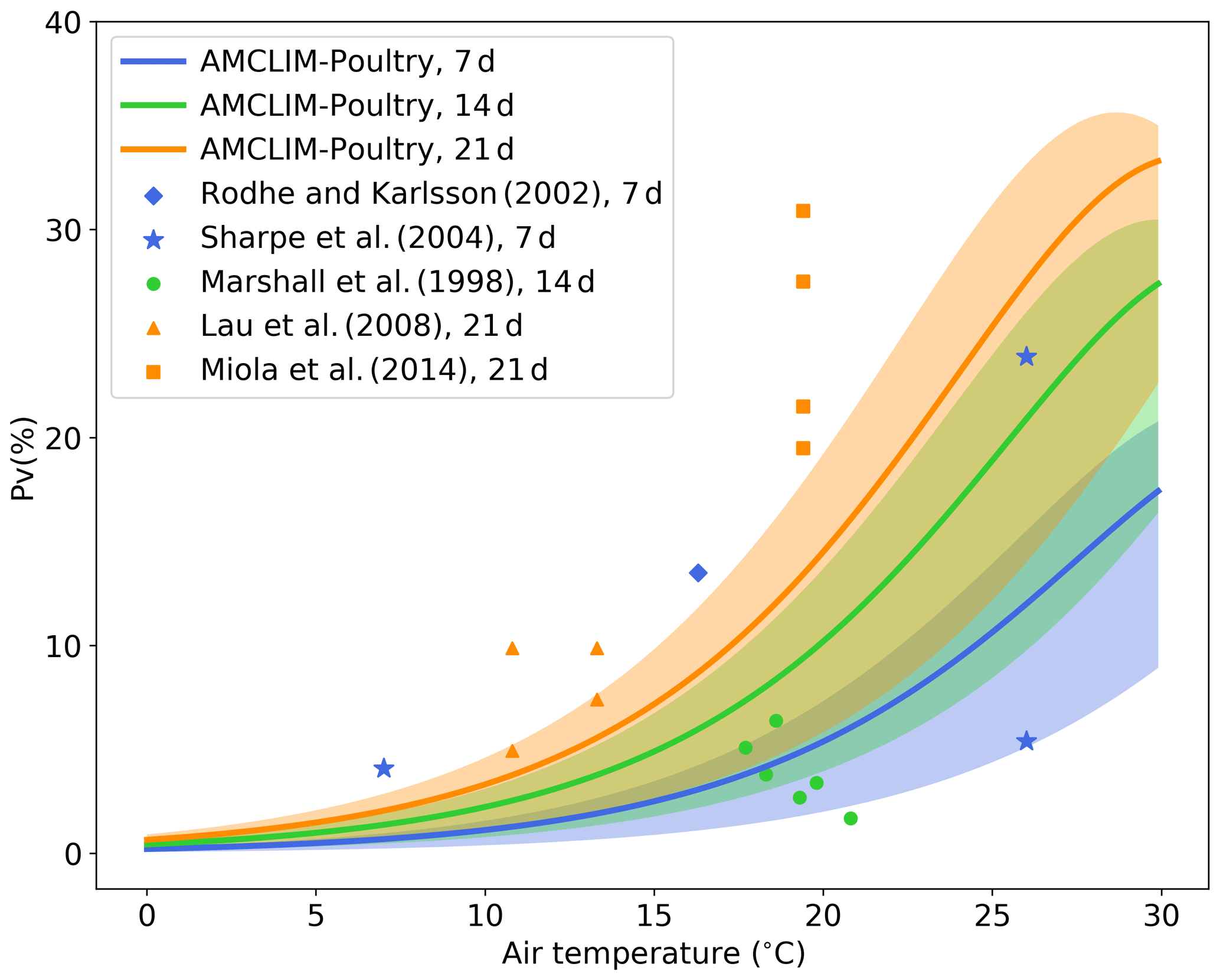
Figure 8 Simulated fraction of total applied nitrogen that is lost as NH₃-N (P_V) as a function of air temperature (in degrees Celsius) by the AMCLIM–Poultry for simulating periods of 7, 14 and 21 d, and a comparison with experimental studies that measured NH₃ N loss for 7, 14 and 21 d. Simulations are conducted for rain-free conditions, where shaded areas indicate the range for simulations from 20 % to 100 % relative humidity. The measured figure of 5 % volatilization at 27 ^∘C by Sharpe et al. (2004) was associated with high precipitation not representative of these simulations.

As shown in Fig. 8, the simulated percentage of nitrogen excreted that is volatilized as NH₃ (P_V) increases as temperature increases because of the faster UA hydrolysis rate in hotter conditions. The shaded areas illustrate ranges of P_V from simulations that use different RH values ranging from 20 % to 100 %, while the solid lines represent the mean P_V rate for the range of RH values for each simulation period (7, 14 and 21 d). Compared with the experimental studies, the model application underestimates NH₃ volatilization for the 21 d simulation and overestimates for the 14 d simulation. However, it is evident that these experimental studies also show large variations, which we expect is especially due to meteorological variation within and between the experimental studies, such as rainfall or windy conditions. For example, at a mean temperature of around 26 ^∘C Sharpe et al. (2004) reported P_V of 23 % and 5 %, respectively. The latter value was caused by a rain event taking place 2 d after application, explaining why the latter point appears low on Fig. 8, where the simulations are based on rain-free conditions. Overall, the model provides P_V rates that fall within the range between 0.5× to 2× compared to the measurements. It should be noted that this is a very simple model experiment because the published experimental studies do not always fully describe environmental conditions, which limits the extent to which features of the AMCLIM–Poultry can be applied for comparison with the measured data sets.

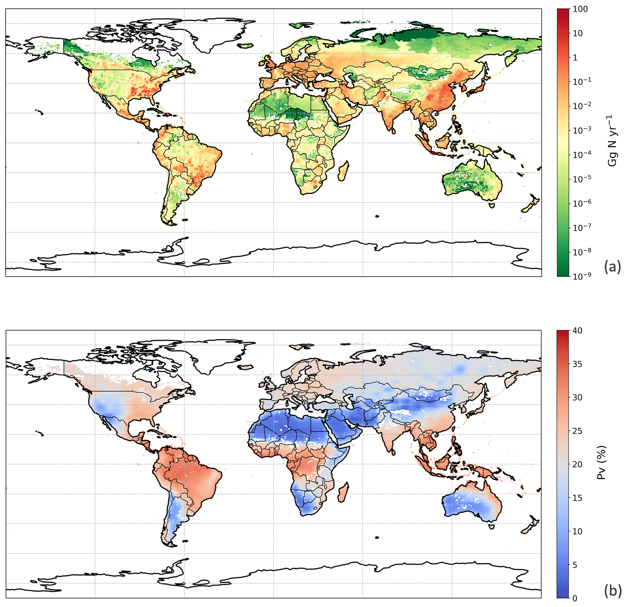
Figure 9 Simulated (a) annual global NH₃ emissions (Gg N yr⁻¹) from chicken housing in 2010. (b) Percentage of excreted nitrogen that volatilizes (P_V) as NH₃ from chicken housing in 2010. The resolution is $\mathrm{0.5}{}^{\circ }\times \mathrm{0.5}{}^{\circ }$. For the simulation shown, the RH parameterization for UA hydrolysis is taken from Elliott and Collins (1984). Figure S9 shows the results of using the RH parameterization, based on new parameterization from AFO monitored data (for comparison).

3.3 NH₃ emission from global chicken housing

We used the polynomial fits shown in Fig. S1 and the constant R^∗ values of 16 700 s m⁻¹ as representative of all chicken houses for the simulation of global emissions. The estimate of NH₃ emission from global chicken housing in 2010 was 2.0 Tg N. This includes 1.3 Tg N emissions from broilers and 0.7 Tg N from layers. Figure 9 shows high emissions in Europe, India, China and Southeast Asia, with emission hot spots in eastern US, and the eastern part of South America. The total amount of nitrogen from chicken excretion was 9.0 Tg N in 2010. The volatilization rate, P_V, was estimated at 22 % overall for all NH₃ emissions from chicken housing globally. The value of P_V for chicken housing was high across the tropics, reaching approximately 35 % (Fig. 9b). Regions with high NH₃ emissions mostly show high NH₃ volatilization rates, especially in regions such as eastern China, Southeast Asia, and eastern US. As the P_V value normalizes for chicken numbers, it more clearly shows the influence of climate than total NH₃ emissions. Figure 9b shows very small P_V values in dry areas (the Sahara, Australia, the Arabian Peninsula, Patagonia, central Asia and western North America), illustrating low humidity in these areas is estimated to limit UA hydrolysis, with the converse in humid areas (Amazonia, central Africa, Southeast Asia, etc.).

3.4 NH₃ emission from global chicken manure spreading

3.4.1 NH₃ emission from chicken manure application for crops

For the year 2010, the NH₃ emission from chicken manure application for crops was 2.7 Tg N, with the P_V value representing 39 % of the total nitrogen application to land of 7.0 Tg N. The nitrogen considered to be left untreated according to Sect. 2.4.3 was less than 50 Gg, which is only a small fraction compared to the amount of nitrogen applied to land. From simulations in this study, over 75 % of the NH₃ emissions were from applications for the major six crops specified in Sect. 2.4.3, while the rest were from applications for other crops (Table S2 in Sect. S7). Among the six crops, maize fertilizing contributed to the highest emission of 676.3 Gg N, which is approximately one-third of the total amount. Fertilizing rice and wheat also led to 641.2 and 542.7 Gg N of emissions, respectively. Compared with maize, rice and wheat, crops of barley, potato and sugar beet had much smaller emissions due to a lower estimated total application of chicken manure to these crops (reflecting their smaller cropping areas and the chicken distribution). The NH₃ volatilization of all six crop types exceeded 35 % (Table S2). The application for rice resulted in the highest P_V of over 43 % (reflecting the warm and moist climate of rice cropping), while the application for barley and sugar beet had the lowest P_V values of 36 % (reflecting its distribution in cooler, temperate climates).

The geographical distribution of NH₃ emissions from chicken manure application is presented in Fig. 10a. Similar to the chicken housing, high emissions can be seen in Europe, the eastern Middle East and southern India, while extremely large NH₃ emissions exceeded 10 Gg N yr⁻¹ over the eastern and central part of China and Southeast Asia, with hot spots in southeastern US, Mexico and eastern South America. These hot spots reflect a combination of high chicken populations and high P_V values. Areas of the lowest P_V are associated with cropping areas having the lowest rainfall, including western central North America, southern Africa and central Asia. Areas estimated to have no significant arable cropping (i.e. desert, boreal and tundra) are shown in white in Fig. 10.

3.4.2 NH₃ emission from backyard chicken

The global NH₃ emission from backyard chicken in 2010 was estimated at 0.7 Tg N from a total excreted nitrogen of 2.2 Tg. Backyard chicken density showed a different distribution compared with broilers and layers (Fig. S10 in Sect. S8). This reflects the assessment in the FAO database that backyard chickens are not kept in developed countries including Canada, the United States of America, western Europe, Australia and New Zealand, where all chickens are allocated to housed systems. The FAO database estimates that most backyard chickens occur in developing regions, such as the northern India and Africa. Geographically, the highest emissions from backyard chickens are here estimated to occur in the Ukraine, southern and southeastern Asia, with high emissions in the eastern coastal regions of South America and the southern part of West Africa. Figure 11b illustrates the geographic distribution of the percentage of nitrogen volatilized (P_V). The volatilization rates of the vast majority of Asia were less than 24 %, while the tropics, including South Asia, had higher P_V rates that reached 36 %. Possible reasons for the different distribution of P_V for backyard birds compared with manure application to crops are discussed in Sect. 4.2.

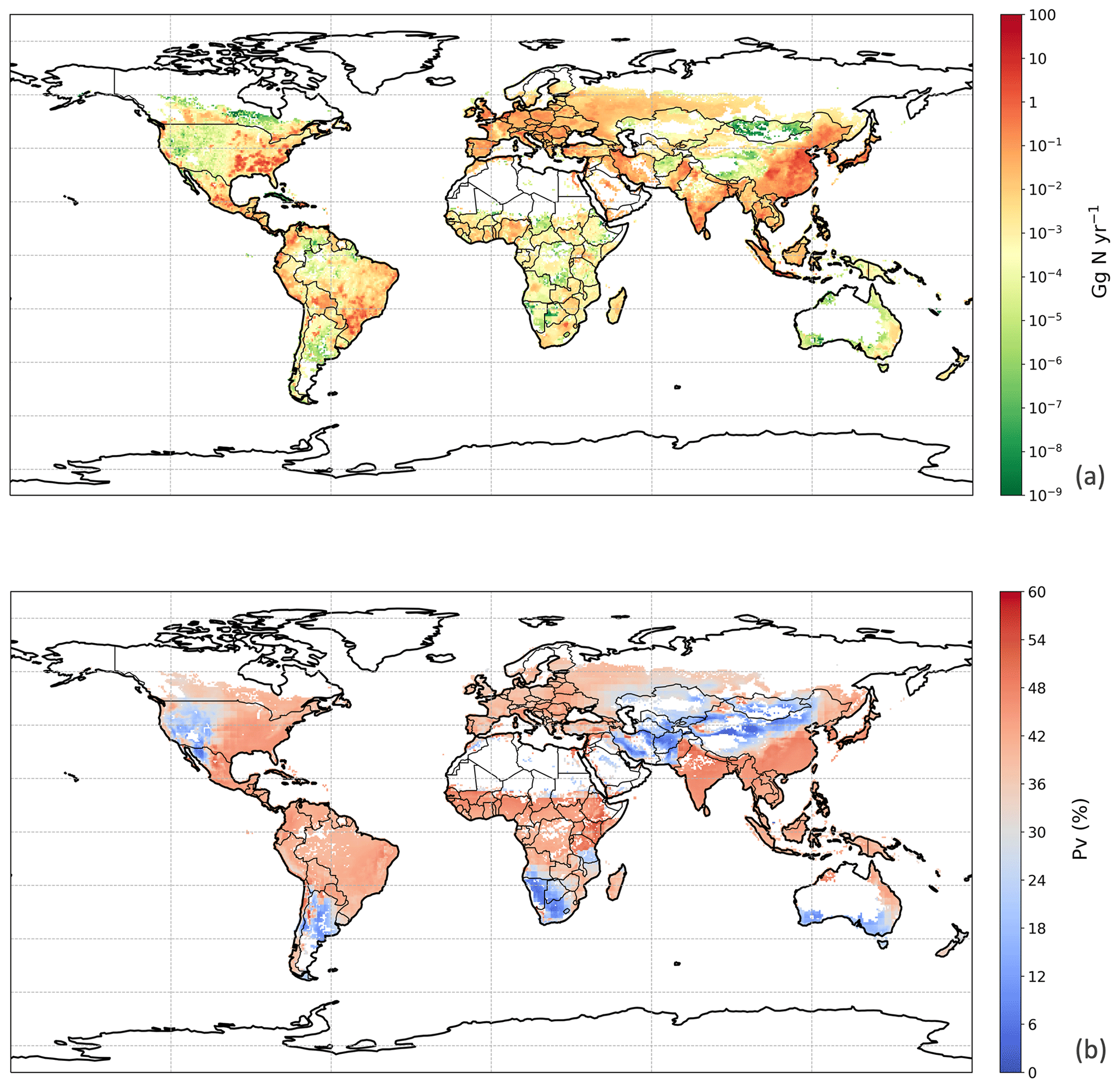
Figure 10 Same as Fig. 9 but for chicken manure application for crops in 2010.

Table 1 Excreted nitrogen from housed and backyard chickens, and estimated annual NH₃ emissions from each practice based on 2010 values.

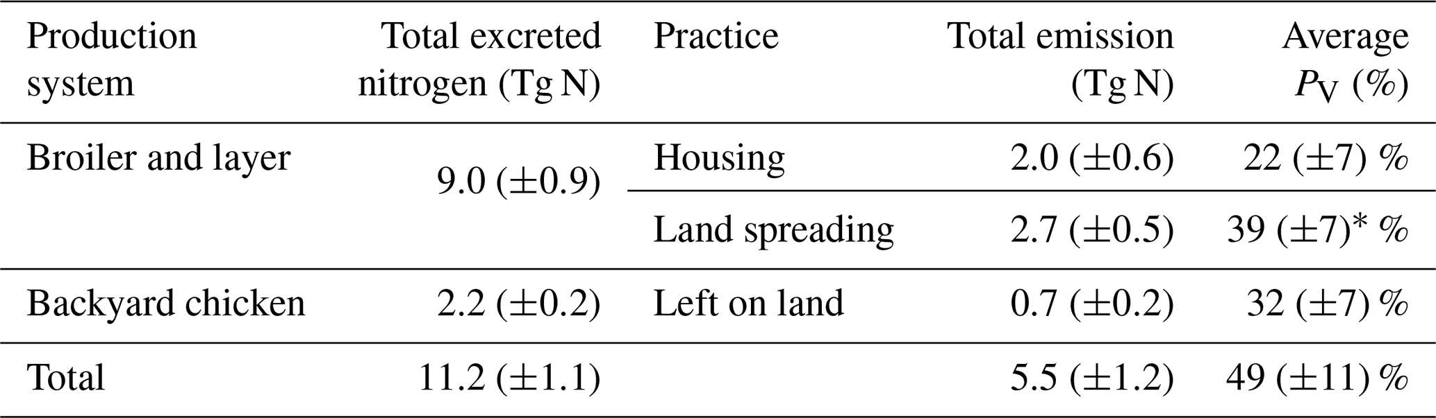
^∗ Average P_V for land spreading is based on the excreted nitrogen remaining (i.e. 7.0 Tg N) after NH₃ volatilization from housing.

3.5 Annual NH₃ emission from global chicken farming

The estimated NH₃ emissions based on 2010 values are summarized in Table 1, and the geographic distribution is presented in Fig. 12. Overall, the total emission from global chicken farming was 5.5 Tg N yr⁻¹. Practice related to broilers and layers, including housing and manure application to crops, contributed 2.2 and 2.7 Tg N NH₃ emissions, respectively, and backyard chicken manure caused 0.7 Tg N emissions. Regions with high NH₃ emissions were found across Europe, India, and parts of China, with hot spots occurring in the eastern US and eastern South America. The distribution of P_V values reflects the combined effect of how environmental differences lead to variations in emissions from chicken housing, manure spreading on arable land and from backyard birds.

Figure 11 Same as Fig. 9 but for backyard chicken in 2010.

Figure 13 shows the NH₃ emissions from the three main components for chickens (housing, crops and backyard) and summarizes the latitudinal difference in percentage volatilized. The highest emissions were identified to occur between 20 and 40^∘ N, reaching a total NH₃ emission of 2.5 Tg N. The lowest emissions accounted for 0.3 Tg N between 20 and 40 ^∘S. Manure application to crops was the largest fraction of NH₃ emissions in the Northern Hemisphere, and its volatilization to NH₃ was the highest among the three categories across the globe, exceeding 35 %. The NH₃ volatilization of housing and backyard chickens were comparable, ranging between 20 % and 30 %. The smaller degree in variation reflects the complex way in which water availability, humidity and temperature interact to affect the overall percentage of nitrogen volatilized, as illustrated by the maps.

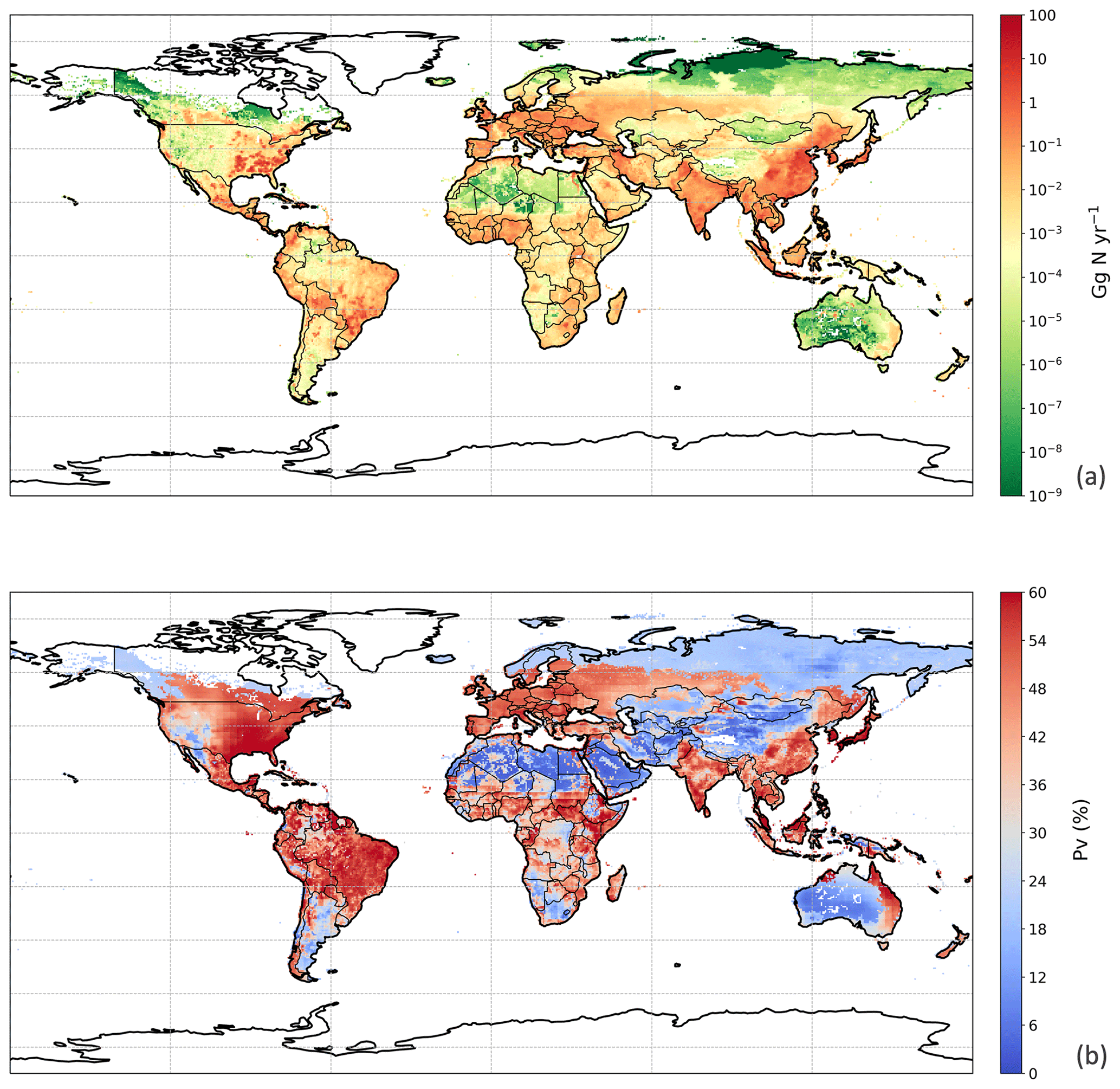
Figure 12 Simulated (a) annual global NH₃ emissions (Gg N yr⁻¹) from chicken agriculture in 2010. (b) Percentage of excreted nitrogen that volatilizes (P_V) as NH₃ from chicken agriculture in 2010. The resolution is $\mathrm{0.5}{}^{\circ }\times \mathrm{0.5}{}^{\circ }$.

Figure 14a shows the monthly NH₃ emissions from each sector. The highest emissions of over 0.6 Tg N were estimated for April and August, while lowest estimated emissions were in November, December and January. This shows how the seasonal differences are larger for NH₃ emissions from manure application than from animal houses, which is a result of both the climatic effects and the temporal distribution of manure application, according to the start of the main cropping seasons. From Fig. 14b, the NH₃ volatilization from backyard chicken excretion varied more throughout the year than for housing (linked to larger variations in temperature and water availability). Emissions from backyard birds were higher than housing from April to August, with the largest difference in July, and were lower than housing from September to March. The highest estimated rate was 65 % in July and the lowest rate was 12 % in January. The volatilization rates of housing showed smaller variations, with P_V values mostly over 20 %, with the highest rate of 28 % occurring in August. It is worth noting that the volatilization rates of manure land spreading are not presented in the figure because simple monthly values do not reflect the true volatilization rate. Nitrogen being applied in the agricultural month will cause NH₃ emissions in the following months when no application practices take place.

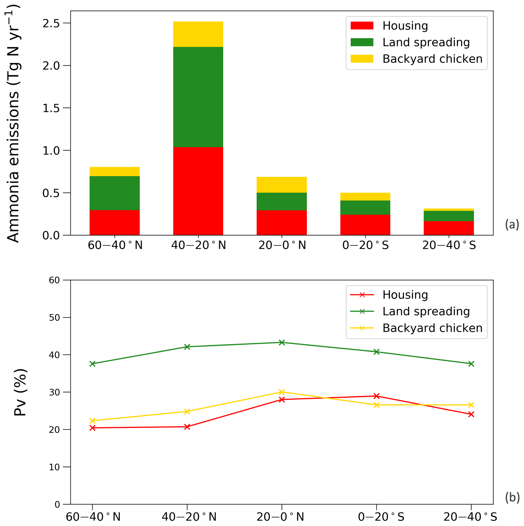
Figure 13 Simulations for chicken housing, manure applications to crops and land spreading of backyard chicken manure in 2010, given in regions. (a) Annual global NH₃ emissions (Tg N yr⁻¹). (b) Percentage of excreted nitrogen that volatilizes (P_V) as NH₃.

4 Discussion

4.1 Model parameterization

4.1.1 UA hydrolysis in chicken housing

Figure 3 shows the parameterizations for UA hydrolysis in chicken houses that are derived from AFO measurements and are taken from Elliott and Collins (1982). The temperature dependences are comparable in that both studies suggest an exponential correlation between the factor T and indoor temperature. Overall, the factor T, derived from using the AFO-monitored data in this study, was slightly larger than that from Elliott and Collins (1982). Within the temperature range of 18 to 28 ^∘C, the UA hydrolysis rate approximately doubled every 5 ^∘C, and an increasing 10 ^∘C led to a more rapid hydrolysis rate by a factor of 4.4 and 5.2, based on the two studies, respectively. In contrast, the RH dependences were more different between the two studies. The new parameterization suggests a linear decline of factor RH as RH decreases below 80 %, so that the magnitudes of factor RH are much larger compared to Elliot and Collins (1982).

The results of the global housing simulations by using two parameterizations are presented in Fig. 9 (using RH parameterization from Elliot and Collins, 1982) and Fig. S9 (using the new RH parameterization based on Fig. 3 from the monitored AFOs). The annual NH₃ emissions from housing in 2010 were estimated at 3.0 Tg N, based on the new parameterization, giving 50 % higher emissions than the estimates of 2.0 Tg N that were obtained by using the equations from Elliott and Collins (1982). In principle, warmer and wetter conditions lead to an increase in P_V. Increasing temperature accelerates the formation of TAN and increases the surface concentration of NH₃, and the hydrolysis of UA is enhanced under high moisture environments. The temperature inside chicken houses in the AMCLIM–Poultry model is assumed to be controlled, especially in the houses in cold climate regions, where sufficient heating is assumed to be used to maintain healthy environments. Therefore, the variations in housing temperature were not as significant as the outdoor temperatures. Meanwhile, the houses prevent rain getting in, so the hydrolysis of UA and aqueous NH₃ concentration are solely restricted by the water content of the excretion, which is a function of RH. As a result, RH becomes the foremost factor that determined the NH₃ emissions by affecting the water availability of the system. It is notable that large differences between the two sets of global simulations (as shown in Figs. 9 and S9 in Sect. S6) occurred in dry regions, such as Northern Africa, the Middle East and Western Australia. Compared with the results of using the Elliott and Collins equations, the new parameterization suggests much higher NH₃ volatilization in dry places. The substantial difference between the model simulations using the two RH parameterizations indicate the need for further data on this relationship. Additional measurement data sets, including both temperature and RH measurements and representing a wider range of environmental conditions, would help to strengthen and extend the relationships observed. The RH dependency of UA hydrolysis from Elliot and Collins (1982) was used for outdoor simulations including land spreading and backyard chickens, which have been previously tested and found to provide robust estimates from the GUANO model (Riddick et al., 2017).

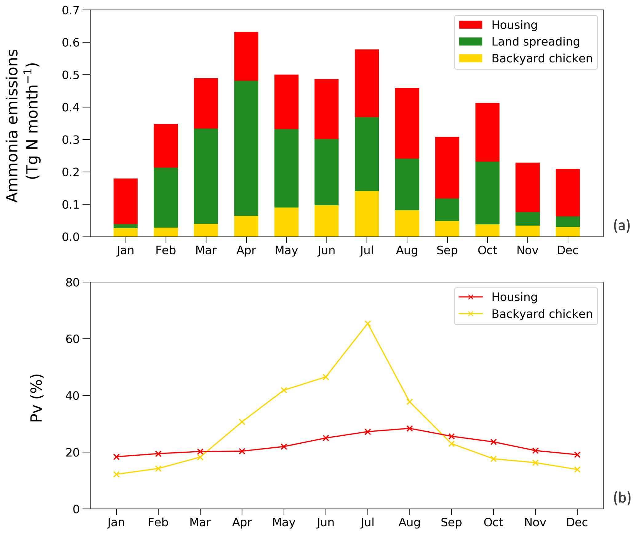
Figure 14 (a) Monthly NH₃ emissions (Tg N yr⁻¹) from chicken housing, manure applications to crops and land spreading of backyard chicken manure in 2010. (b) Percentage of excreted nitrogen that volatilizes (P_V) as NH₃ monthly for chicken housing and land spreading of backyard chicken manure.

It must also be recognized that both the RH parameterizations shown in Fig. 3b have limitations. A more accurate parameterization of RH dependence might fall in the area between two curves in Fig. 3b. It can be seen from Figs. 4c and 5c that the TAN pool of each chicken house increased continuously throughout the simulation period rather than remaining approximately constant at some points. This indicates that the TAN produced exceeded the loss through NH₃ emission, which is against the assumption that the production of TAN is equivalent to the NH₃ emission. It is possible that the new RH dependence overestimated the rate of UA hydrolysis. Meanwhile, from Figs. S4 and S5, by using Elliott and Collins' (1982) equation, the modelled indoor concentration of NH₃ was much lower than the measurements during the starting period of the simulations. This indicates an insufficient TAN pool that limited the emissions. Therefore, Elliott and Collins' (1982) parameterization probably underestimated the TAN production from UA hydrolysis, especially when each nitrogen pool was limited. In addition to the need for further data sets that relate NH₃ emissions from housed chicken to both indoor temperature and relative humidity, parallel measurements of the water, UA and TAN content and pH of different litter layers would be helpful for improving future parameterization.

4.1.2 Implications for the idealized simulations

As shown in Figs. 6 and 7, it can be seen from dry simulations (i.e. without precipitation) under idealized conditions for a whole year run that the annual mean P_V was relatively small and can drop to approximately zero when temperature is low. It indicates that the UA hydrolysis is hardly taking place. In contrast, the P_V was much higher in hot and wet regimes, reflecting an effective hydrolysis of UA. It is notable that the P_V declines at very high RH levels, using the new RH parameterization. This is mainly because the UA hydrolysis is considered to be optimum at 80 % and higher RH, but the TAN concentration becomes lower as the excretion contains more water when the ambient environment is humid, thereby providing a diluting effect.

From Fig. 7a, the P_V rate is seen to grow exponentially as a function of temperature for the 20 % RH simulations. It is similar to the impact of temperature on UA hydrolysis and also the Henry's law relationship. Conversely, for a humid environment with RH at 100 %, there is a smaller increase in P_V, showing a logarithmic-like trend. These differences are consistent with different amounts of TAN under the two cases. When there is sufficient TAN produced from the UA hydrolysis, the resistance can become the key limiting factor to emissions from the system. Conversely, in low-humidity environments, as the UA hydrolysis is limited, the produced TAN is readily removed through the atmospheric release of NH₃, with the total emission limited by the UA hydrolysis rate. Therefore, the rise in temperature under dry conditions provides a larger increase in NH₃ emissions.

From Fig. 7b, it is worth noting that the decrease in P_V occurs when the RH slightly exceeds 90 % rather than 80 %. A more obvious, sharp decline can be seen from the 15 ^∘C simulations. As discussed, there is a diluting effect on the TAN concentration when the RH is over a certain level. The possible reason why this turning point does not occur at 80 % RH, where the factor RH reaches the optimum, can be summarized as follows. The P_V rates in these simulations represent the integral of a whole year. The diluting of more water to dissolve TAN at high RH affects the instantaneous emission without changing the amount of the TAN pool. Low emissions in the earlier stage can therefore cause a larger emission potential in the later stage due to accumulation of TAN.

The overall implication of these idealized simulations is to demonstrate the close interplay between water availability and temperature, where temperature always increases volatilization (partitioning in favour of the gas phase), whereas a small amount of water is needed to facilitate UA hydrolysis, increasing the NH₃ emissions, while excess water availability dilutes the TAN pool, thereby reducing NH₃ emissions. These same principles also apply for emissions from manure application to crops and for backyard birds, where precipitation and run-off become more important.

4.2 Spatial and temporal variations of NH₃ emission

The NH₃ emission from chicken agriculture differs substantially across regions, both because of different chicken number distributions (Fig. S10), as this affects total nitrogen excretion, and because of different volatilization rates, as shown by the P_V values. The largest NH₃ emission is calculated for regions between 20 and 40^∘ N, which corresponds to the highest chicken density and associated manure application to land. The animal number and the amount of nitrogen from excretion have a first-order effect on the magnitude of emissions. Considering the P_V, the most significant spatial variations relate to emissions from manure spreading and backyard chickens, with less spatial variation in P_V for housed birds as the indoor conditions are considered to be largely controlled. The P_V rates of backyard chicken excretion were much lower in China and Southeast Asia in comparison with manure land application because the wash off is a major loss of nitrogen pools in these regions, especially during non-cropping periods when chicken manure is not applied to land (according to our model approach), while backyard birds lead to outdoor NH₃ emissions all year round (including during non-cropping periods with high precipitation).

It should be noted that from the northern India to Tibet, the P_V rate declines sharply from 40 % to below 6 % from all categories. This indicates that a sudden change from hot and wet conditions to cold and dry conditions causes the volatilization rate to drop dramatically in Tibet compared with India. This example clearly illustrates how the fraction of nitrogen volatilized as NH₃ is strongly linked to meteorological and related environmental conditions.

The AMCLIM–Poultry simulations also showed strong seasonal variations in NH₃ emissions from manure land spreading and backyard chicken excretion. The seasonal distributions (as illustrated by Fig. 14) were caused by changes in meteorological conditions, with high NH₃ emissions in summer due to the high temperatures influencing NH₃ emissions from housing and backyard birds. Even larger seasonal differences are seen in the modelled emission estimates for the land application of manure because this combines both the direct effects of environmental variation (temperature and water effect on P_V) with seasonal differences in the estimated timing of manure application to the land. Paulot et al. (2014) found that maximum NH₃ emissions from manure fertilizing can occur from April to September, depending on the local management. For example, they found that emission peaks in spring occurred in Europe, while summer emission peaks occurred in parts of the US and China. These differences reflect a combination of agricultural timing and the meteorological/environmental drivers (Hertel et al., 2011). Riddick et al. (2016) also showed the maximum emissions usually occur in April–June or July–September. The findings in present study are broadly consistent and demonstrate for the first time, on a global scale, how emissions from managed poultry (chicken) are dependent on both short-term meteorology and long-term regional climatic differences. Contrary to manure spreading and backyard birds, the seasonal variations in NH₃ emissions from chicken housing were much smaller due to the partly controlled environment and the assumed absence of precipitation/run-off within the houses.

Table 2 Estimates of NH₃ emissions from poultry/chicken farming by the Integrated Database model for Agricultural emissions (IDA; Albrektsen et al., 2017) for Denmark, by the National Ammonia Reduction Strategy Evaluation System (NARSES; Misselbrook et al., 2011) for the United Kingdom, based on 2010 values, and by the National Emission Model for Ammonia (NEMA; Velthof et al., 2012) for the Netherlands, based on 2009^∗ values. Ranges given in the P_V housing represent the geographical variations across the country.

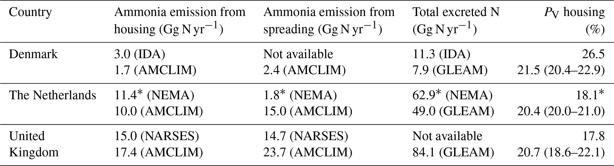
^∗ Based on 2009 values.

4.3 Comparison with other inventories and models

We compared the results from the AMCLIM–Poultry model to three other (model-based) studies/reports from Denmark, the Netherlands and the United Kingdom, respectively. The Danish IDA model (Albrektsen et al., 2017) and the UK NARSES model (Misselbrook et al., 2011) provided 2010 emission data, and the NEMA model (Velthof et al., 2012) from the Netherlands provided estimate emissions from 2009 (see Table 2). All these studies report emissions from poultry rather than chicken. It has been clearly stated that the inputs used in the AMCLIM–Poultry from the GLEAM model and also used here are chicken data, which excluded other poultry such as turkeys, ducks, etc. Therefore, we can see that the excreted nitrogen from the GLEAM model (GLEAM; FAO, 2018) is generally smaller than other individual studies. For housing, the AMCLIM model shows similar estimates of NH₃ emissions to the other models. The housing emissions from this study are smaller than the local models in Denmark and the Netherlands, partly due to the smaller total excreted nitrogen from the animals. However, the AMCLIM model suggests larger emissions from land spreading for the Netherlands and the UK (spreading-derived emissions are not available from the IDA model), especially in the Netherlands where the difference between the two estimates reaches eight times. This is probably due to the different schemes or assumptions for land spreading practices, e.g. deep injection of manure, in different models. The P_V rates, which indicate the fraction of nitrogen that is emitted as NH₃, are comparable from all models for the housing sector. The AMCLIM model suggests that the P_V rates do not vary significantly between these countries because the indoor conditions are largely controlled and in similar climates, which leads to small variations in house environments.

In addition, we also compared our results with existing emission factors (EFs). On a global average, the AMCLIM model estimated that the EFs for broiler and layer housing are 0.13 and 0.10 kg of N per animal per year, respectively. Combining with emissions from land application, the total EFs are 0.30 and 0.27 kg of N per animal per year for broilers and layers, and the EF for backyard chicken is 0.19 kg of N per animal per year. Regionally, the AMCLIM model estimates that the UK have EFs of 0.13 (0.11–0.14) kg of N per animal per year for chicken housing and 0.30 (0.12–0.33) kg of N per animal per year for the total emission, compared to 0.10 (0.06–0.15) for housing and 0.22 (0.15–0.30) for the total EF reviewed by Sutton et al. (1995a). For Europe, the EFs estimated by the AMCLIM model are 0.10 (0.01–0.16) and 0.09 (0.01–0.15) kg of N per animal per year for broiler and layer housing, and 0.15 (0.01–0.28) kg of N per animal per year for the followed land application. In comparison, according to the European Monitoring and Evaluation Programme and European Environmental Agency (EMEP/EEA, 2019), EFs are 0.16 to 0.32 and 0.15 kg of N per animal per year for layer housing and consequent manure application, while EFs for broiler housing and manure application are 0.13 and 0.04 kg of N per animal per year.

Table 3 Sensitivity test for model parameters for global application of the model.

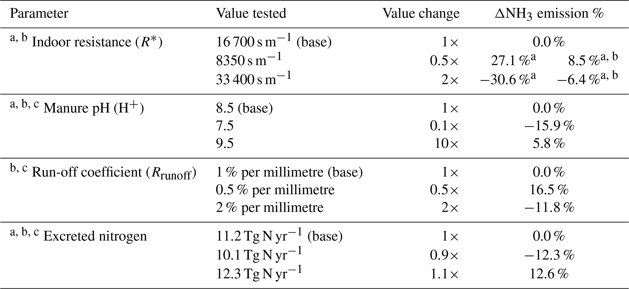
^a Parameters affecting NH₃ emissions from housing. ^b Parameters affecting NH₃ emissions from land spreading of chicken manure. ^c Parameters affecting NH₃ emissions from backyard chicken.

4.4 Uncertainty and limitations

There is substantial uncertainty in modelling NH₃ emissions from livestock farming. Here, we focus on discussing the uncertainty related to model parameterizations. The model parameters may influence the emissions interactively with non-linear consequences. We find that it is helpful to conduct a sensitivity analysis by simulating the effect of the changes in parameters on NH₃ emissions. By doing this, we are able to indicate the ranges of uncertainty and also to highlight which parameters are most important and need to be further investigated. Based on prior test, we find that indoor resistance R^∗, manure pH, run-off coefficient and amount of N excreted are most important, and we examine these in the sensitivity tests, with results summarized in Table 3. In addition, the uncertainty arising from the parameterization of UA hydrolysis is represented by the differences between Figs. 9 and S9.

It is worth noting that the ranges of the parameters are based on expert judgement. Indoor resistance and run-off coefficients are considered to be uncertain by a factor of 2, with manure pH uncertain by ±1, which corresponds to a factor of 10 for hydrogen ion concentrations. The nitrogen excretion rate is considered to have an uncertainty of 10 %. The global simulation of housing driven by varying indoor resistance values shows that R^∗ that is two times higher leads to an NH₃ emission decrease by approximately 31 % and two times lower R^∗ leads to 27 % higher emissions, which is similar to the result at the site scale (see Fig. S8). The R^∗ values directly influence the magnitude of housing emissions but only to a limited extent. The R^∗ values also impact NH₃ emissions from land spreading of chicken manure by limiting the available amount of nitrogen that is applied to land. In total, doubling R^∗ leads to a reduction in NH₃ emissions by 6.4 %, and halving R^∗ leads to an increase in emissions by 8.5 %. The manure pH, which affects the hydrolysis rate of UA and the chemical equilibria between NH${}_{\mathrm{4}}^{+}$ and gaseous NH₃, is found to have positive effect on NH₃ emissions so that emissions tend to increase as pH increases. We find that increasing pH from 8.5 to 9.5 causes annual NH₃ emissions to increase by 5.8 %, while a decrease in pH to 7.5 leads to a decline in emissions by 15.9 %. The run-off coefficient was set to be 1 % per millimetre for nitrogen pools in the model (Riddick et al., 2017). By doubling the run-off coefficient, the NH₃ emissions decrease by 11.8 %, while decreasing the coefficient to half leads to emissions increasing by 16.5 %. It should be noted that, among these parameters, changing the manure pH has influences on both housing emissions (from broiler and layer housing) and outdoor emissions (spreading of broiler and layer manure; backyard chicken manure). The run-off coefficient only affects the outdoor emissions, while indoor resistances limit housing emissions directly but also have impacts on consequent outdoor emissions. Smaller NH₃ emissions from housing indicate a larger potential for outdoor release during the spreading stages under the same farming practices. Conversely, higher housing emissions lead to smaller consequent emissions from land application. Concerning the nitrogen excretion rate from chickens, we find that 10 % in variation leads to an annual NH₃ emissions change of approximately 12 %. The change in NH₃ emissions is not proportional to the nitrogen input because of non-linear interactions in the model, e.g. an increase in nitrogen input by 10 % may only lead NH₃ emissions to increase by a negligible amount in regions with heavy rainfall. Combining these ranges and taking the base run result as the best estimate, the overall expected uncertainty of NH₃ emissions from global chicken farming is 1.2 Tg N yr⁻¹, where component uncertainties of housing, land spreading and backyard chicken are 0.6, 0.5 and 0.2 Tg N yr⁻¹, respectively. Detailed estimates are described in Sect. S9.

Future directions of the study include (a) a better parameterization for UA hydrolysis, (b) developing an interactive scheme for soil interactions, which allows us to simulate soil pH dynamically and identify relevant soil processes such as the absorption of TAN, (c) incorporate more detailed pathways for nitrogen flows, such as nitrification and leaching and canopy recapture, and (d) a better representation of human management based on statistical data or national and international survey.

4.5 Potential for considering NH₃ mitigation scenarios

The process-based approach of the AMCLIM–Poultry model lends itself well to the opportunity to assess the implementation of possible management options to abate NH₃ emissions. Of the many measures for reducing NH₃ emissions as described by the United Nations Economic Commission for Europe (UNECE; Bittman et al., 2014), several of them could be incorporated as part of future model development, for example, the following points:

• a.

  Measures to optimize animal diets to reduce excretion per animal. Such measures could be incorporated in the estimated amount of excretion per bird.

• b.

  Measures to reduce moisture in poultry houses and reduce UA hydrolysis. Such measures could be incorporated into the relationship between indoor and outdoor conditions for relative humidity.

• c.

  Measures to reduce the temperature of stored manure and reduce UA hydrolysis and NH₃ emission. Such measures could be included in a possible future AMCLIM module on manure storage by altering the model temperature.

• d.

  Measures to alter the timing of manure application to favour land application under cool conditions. This could be included by altering assumed ambient temperatures compared with seasonal averages.

• e.

  Measures to incorporate poultry manure immediately into the soil. This could be included empirically, based on an alteration of atmospheric transfer resistances, or by a more detailed development of several vertical layers or the model nitrogen pools (see Riedo et al., 2002).

While such considerations represent opportunities for future work, they highlight how the AMCLIM–Poultry model is well suited to the consideration of NH₃ emissions abatement scenarios.

5 Conclusions

This paper presented the simulated NH₃ emissions from global chicken farming by using the AMCLIM–Poultry model, including considerations of meteorological effects and simplified agricultural practices. The AMCLIM–Poultry model was designed based on underlying physics and chemistry, supported by evidence from experimental studies.

The magnitude of total NH₃ emissions from chicken farming estimated by the AMCLIM–Poultry based on 2010 was 5.5 ± 1.2 Tg N yr⁻¹, which accounts for approximately 13 ± 3 % of agriculture-derived NH₃ emissions (Crippa et al., 2016). High NH₃ emissions were from southern and eastern Asia, Europe and southeastern US. These regions also had high NH₃ volatilization rates, expressed as the percentage of excreted nitrogen (P_V) that is volatilized as NH₃. The tropics often had high P_V values, being up to five times higher than cold or dry regions, which illustrates how large NH₃ emission potentials are expected under hot and wet conditions. Agricultural activities related to chicken represent appreciable NH₃ sources, indicating that currently increasing NH₃ emissions, accompanied by increasing chicken density (FAO, 2018), is important – especially as climate change is also expected to increase NH₃ emissions, as demonstrated by the spatial comparisons of the model.

Based on 2010 values, the model estimated that 22 % of the total excreted nitrogen was volatilized as NH₃ emissions from chicken housing. The total NH₃ emission was 2.0 Tg N, where 1.3 Tg N was from broilers and 0.7 Tg N was from layers. For the land-based emissions, global NH₃ emissions were 2.7 Tg N from manure fertilizer applications for crops and 0.7 Tg N from backyard chicken excretion, respectively, with strong spatial and temporal variations. In the current model approach, NH₃ emissions from manure storage are incorporated as in-house storage with housing emissions. Further information on variations in practices is needed as a basis to estimate NH₃ emissions from the outdoor storage of chicken manure, although the overall climate effect is expected to be midway between that for housing (covered outdoor storage) and land spreading (uncovered storage). Contrary to empirical approaches, this study uses a process-based method to quantify NH₃ emissions from chickens, which provides a foundation for estimating emissions from other livestock types, based on theoretical considerations. The calculation of P_V values is an asset of the model, which provides insight to how environmental interactions will affect the NH₃ emissions and which could also be applied for considering scenarios using emission abatement options. Strong spatial variation in P_V implies that a single, empirically derived emission factor would not usually reflect reality under different climate conditions. The results of this study show increased emissions under warm conditions, pointing to an expectation that climate change will increase chicken NH₃ emissions globally. The different relationships for housed chickens (primarily temperature and humidity dependence) and for backyard birds and manure spreading (primarily temperature and precipitation dependence) indicate that the net effect of climate change on regional emissions will depend on the relative composition of chicken types and management.

Appendix A

Abbreviation	Unit	Model Variable
fN	g N g excretion−1	N content of chicken excretion
fUA		Fraction of uric acid in chicken excretion
Fe	g N m−2 s−1	Total nitrogen excretion rate from chicken
$F_{{\mathrm{H}}_{\mathrm{2}}\mathrm{O}}$(evap)	g m−2 s−1	Evaporation
$F_{{\mathrm{H}}_{\mathrm{2}}\mathrm{O}}$(rain)	g m−2 s−1	Precipitation
$F_{{\mathrm{NH}}_{\mathrm{3}}}$	g N m−2 s−1	Net rate of conversion of TAN to gaseous NH3 within litter/manure
Fremoval	g N s−1	Removal of NH3 through ventilation in the chicken house
Fsurface	g N s−1	Total flux of NH3 from surface litter in the chicken house
FTAN	g N m−2 s−1	Flux of TAN from uric acid hydrolysis
K(T, pH and RH)	s−1	Function of temperature, pH and RH influencing uric acid hydrolysis rate
kpH		Function of pH influencing uric acid hydrolysis rate
kRH		Function of RH influencing uric acid hydrolysis rate
kT		Function of temperature influencing uric acid hydrolysis rate
mE		Equilibrium moisture content of litter/manure
Mavailable water	g m−2	Mass of water in the system that is available for wash off
Mexcretion	g m−2	Mass of excretion
$M_{{\mathrm{H}}_{\mathrm{2}}\mathrm{O}}$	g m−2	Mass of water in the system
$M_{{\mathrm{H}}_{\mathrm{2}}\mathrm{O}}$(e)	g m−2	Mass of water in the excretion
MN	g N m−2	Mass of nitrogen components
MN-runoff	g N m−2	Mass of instant run-off for nitrogen components
MTAN	g N m−2	Mass of nitrogen in the form of TAN
MUA	g N m−2	Mass of nitrogen in the form of uric acid
NCrop	g N m−2	Amount of total N application for individual crops
NCrop_Chicken	g N m−2	Amount of chicken manure N application for individual crops
NAvailable	g N m−2	Amount of available chicken manure N
NTotal_manure	g N m−2	Amount of total N application for all crops
pH		pH of litter/manure
Q	m3 s−1	Ventilation rate in chicken house
Qavailable water	mm	Pools of water in the system that are available for wash off
rN	mm−1	Wash-off factor
Rrunoff		Run-off coefficient
R∗	s m−1	Overall indoor resistance in the chicken house
Ra	s m−1	Aerodynamic resistance
Rb	s m−1	Boundary layer resistance
RH	%	Relative humidity
S	m2	Surface area of the chicken house
T	K	Ground temperature
V	m3	Volume of the chicken house
$V_{{\mathrm{H}}_{\mathrm{2}}\mathrm{O}}$	mL m−2	Volume of water in the manure
z	m	Reference height
χin	g m−3	Air concentration of NH3 in the chicken house
χout	g m−3	Air concentration of NH3 of ambient environment
χsurface	g m−3	Concentration of NH3 in litter/manure on the surface