the Creative Commons Attribution 4.0 License.
the Creative Commons Attribution 4.0 License.
 | 16 Apr 2021
Functional convergence of biosphere–atmosphere interactions in response to meteorological conditions
Mirco Migliavacca
Diego G. Miralles
Guido Kraemer
Tarek S. El-Madany
Markus Reichstein
Jakob Runge
Miguel D. Mahecha
Understanding the dependencies of the terrestrial carbon and water cycle with meteorological conditions is a prerequisite to anticipate their behaviour under climate change conditions. However, terrestrial ecosystems and the atmosphere interact via a multitude of variables across temporal and spatial scales. Additionally these interactions might differ among vegetation types or climatic regions. Today, novel algorithms aim to disentangle the causal structure behind such interactions from empirical data. The estimated causal structures can be interpreted as networks, where nodes represent relevant meteorological variables or land-surface fluxes and the links represent the dependencies among them (possibly including time lags and link strength). Here we derived causal networks for different seasons at 119 eddy covariance flux tower observations in the FLUXNET network. We show that the networks of biosphere–atmosphere interactions are strongly shaped by meteorological conditions. For example, we find that temperate and high-latitude ecosystems during peak productivity exhibit biosphere–atmosphere interaction networks very similar to tropical forests. In times of anomalous conditions like droughts though, both ecosystems behave more like typical Mediterranean ecosystems during their dry season. Our results demonstrate that ecosystems from different climate zones or vegetation types have similar biosphere–atmosphere interactions if their meteorological conditions are similar. We anticipate our analysis to foster the use of network approaches, as they allow for a more comprehensive understanding of the state of ecosystem functioning. Long-term or even irreversible changes in network structure are rare and thus can be indicators of fundamental functional ecosystem shifts.
- Article
(16766 KB) - Full-text XML
- BibTeX
- EndNote


Terrestrial ecosystems and the atmosphere constantly exchange energy, matter, and momentum (Bonan, 2015). These interactions result in biosphere–atmosphere fluxes (in particular carbon, water, and energy fluxes) that are shaped by a variety of climatic conditions and states of the terrestrial biosphere (McPherson, 2007). Understanding how biosphere–atmosphere fluxes interact and how they causally depend on the short-term meteorological and long-term climate conditions is crucial for building predictive terrestrial-biosphere models (Detto et al., 2012; Green et al., 2017). However, the exact causal structure of dependencies between surface and atmosphere variables is still subject to unknowns (Baldocchi et al., 2016; Miralles et al., 2019). For example, we still do not understand well under which conditions certain climate extremes turn ecosystems into carbon sources or sinks (Sippel et al., 2017; Flach et al., 2018; von Buttlar et al., 2018). One reason for our incomplete understanding is that the causal dependencies underlying biosphere–atmosphere interactions might vary among ecosystems depending on vegetation structure and its long-term adaptation to climatic conditions.
Conducting a comparative study across ecosystems, focusing on their interactions with the atmosphere, has two requirements: firstly, we need standardised data encoding biosphere fluxes and meteorological conditions. Secondly, an analytical tool is needed that extracts an interaction structure from these data empirically. The latter requires handling of multivariate processes and estimating dependencies beyond correlations. The first requirement is best met by the FLUXNET database (Baldocchi, 2014), a collection of global long-term observations of biosphere–atmosphere fluxes measured via the eddy covariance method (Aubinet et al., 2012). The spatial distribution of FLUXNET sites is biased to European and North American sites, yet it still covers most climate zones and vegetation types ranging from boreal steppe to tropical rainforests surprisingly well (Reichstein et al., 2014). Further, the data are processed homogeneously across sites. The second requirement is addressed by causal inference. Various methods exist today (see Runge et al., 2019a, for a recent overview), some of which have been applied already in the biogeosciences (Ruddell and Kumar, 2009; Detto et al., 2012; Green et al., 2017; Papagiannopoulou et al., 2017; Shadaydeh et al., 2019; Claessen et al., 2019). One of that group is PCMCI (Runge et al., 2019b), a causal graph discovery algorithm based on a combination of the PC algorithm (named after its inventors, Peter and Clark; Spirtes and Glymour, 1991) and the test of momentary conditional independence (MCI) (Runge et al., 2019b). By applying such tests, it becomes possible to account for common drivers and mediators which can cause two variables to correlate even though no direct causal link exists between them. Then MCI partial correlations estimated by PCMCI yield a better interpretation of the strength of a causal mechanism than the common Pearson correlation. Krich et al. (2020) tested PCMCI regarding its suitability for interpreting eddy covariance data. The method proved to be consistent despite the data's inherent noisy character and was capable of extracting well-interpretable interaction structures. A causal interpretation of specific links, though, has to take into account regarding potentially unmet assumptions.
In this study, we investigate multivariate time series from FLUXNET tower data to understand how networks of biosphere–atmosphere interactions vary across vegetation types and climate zones. The rationale is as follows: if biosphere–atmosphere interactions varied significantly across climate gradients or between vegetation types, this could indicate, for example, that ecosystem responses to climatic extremes could differ significantly and would require terrestrial-biosphere models to account for them differently. If, however, the opposite applies and ecosystems of the Earth exhibit similar biosphere–atmosphere interaction types, then common principles can be identified that can serve as empirical reference for global vegetation models. We hypothesise first that the accessible states of biosphere–atmosphere interactions are limited and can be characterised by few functional states despite the complexity and differences among ecosystems. Second, attributing to an ecosystem's adaptation, we further hypothesise that a specific ecosystem can only access a limited fraction of the functional states.
The study is designed as follows: firstly, we perform causal discovery by PCMCI at each eddy covariance site and season. Secondly, we solely investigate the resulting interaction networks and visualise them in a low-dimensional space. We then interpret the low-dimensional space of biosphere–atmosphere interactions and investigate seasonal cycles, characteristic states, and the role of vegetation types and finally discuss the potential role of adaptation to the underlying climate space.
2.1 Eddy covariance observations
We used eddy covariance data from the FLUXNET database (Baldocchi et al., 2001) aggregated to daily time resolution. To maximise the available ecosystems and time series length, we took the union of the LaThuile fair-use (Baldocchi, 2008) and FLUXNET2015 Tier 1 (Pastorello et al., 2020) datasets (Nelson et al., 2020) with at least 5 years of measurement. If a site year was available in both datasets, we selected the one from FLUXNET2015. A detailed list of used sites and years is given in Table . The final dataset contains 119 sites from the major plant functional types and covers the major Köppen–Geiger climate classes, i.e. tropical to polar climate zones. The majority of sites belong to evergreen needleleaf forests, grasslands, and deciduous broadleaf forests. The dominant climate classes are continental, temperate, and dry climates. The dataset's variables, including meteorological and eddy covariance measurements, were quality-checked, filtered, gap-filled, and partitioned with standard tools (Papale et al., 2006; Pastorello et al., 2020) and provided with per-variable quality flags. We extracted the following variables, comparable between the two datasets, and their corresponding quality controls (if available): short-wave downward radiation (or global radiation, Rg), air temperature (T), net ecosystem exchange (NEE) (inverted so that positive values signify carbon uptake into the biosphere), vapour pressure deficit (VPD), sensible heat (H), latent heat flux (LE), gross primary productivity (GPP), precipitation (P), and soil water content (SWC, measured at the shallowest sensor). Within the FLUXNET2015 dataset these variables are named as “SW_IN_F_MDS”, “TA_F_MDS”, “NEE_VUT_USTAR50”, “VPD_F_MDS”, “H_F_MDS”, “LE_F_MDS”, “GPP_NT_VUT_USTAR50”, “P”, and “SWC_F_MDS_1”, respectively. Correspondingly for the LaThuile dataset they are “Rg_f”, “Tair_f”, “NEE_f”, “VPD_f”, “LE_f”, “H_f”, “GPP_f”, “precip”, and “SWC1_f”, respectively. GPP is calculated via the commonly used nighttime flux partitioning (Reichstein et al., 2005). Here GPP is the difference between ecosystem respiration and NEE. The latter is estimated via a model which is parameterised using nighttime values of NEE.
2.2 PCMCI
To analyse biosphere–atmosphere interactions, we estimated network structures using the causal-network discovery algorithm PCMCI. PCMCI is tailored to estimate time-lagged dependencies from potentially high-dimensional and autocorrelated multivariate time series. Dependencies can be interpreted causally under certain assumptions. The algorithm is explained from a biogeoscientific viewpoint in Krich et al. (2020). A comprehensive description from theoretical assumptions to numerical experiments is given in Runge et al. (2019b). As a brief summary, PCMCI efficiently conducts conditional independence tests among variables to reconstruct a dependency network. While PCMCI can also be combined with non-linear tests, here we estimate conditional independence using partial correlation (ParCorr), implying that we only consider linear dependencies. Partial correlation between two variables X and Y given a variable set Z is defined as the correlation between the residuals of X and Y after regressing out the (potentially multivariate) conditions Z. The conditions Z can consist of lagged third variables or time lags of X and Y.
PCMCI has two phases. In the first phase, the “condition selection”, a superset of lagged parents (up to some maximum time lag τmax) of each variable is estimated based on a fast variant of the PC algorithm (Spirtes and Glymour, 1991). A parent of is any lagged variable that is directly influencing . This can be the own past, i=j, τ>0, or other variables, i≠j, τ>0. A pseudo-code of this procedure is given in the Supplement of Runge et al. (2019b). In the second phase, “momentary conditional independence” (MCI) is estimated among all pairs of contemporaneous and lagged variables (, ) for τ≥0. The MCI test removes the influence of the lagged drivers (obtained in the first phase) using ParCorr and yields link strengths and p values (based on a two-sided t test). The link strength is here given by the MCI partial correlation. In short, the MCI value gives an estimate of dependence between two time series, one potentially lagged, with the influence of other lagged drivers including autocorrelation removed, yielding a better interpretation of the strength of a causal mechanism than the common Pearson correlation. For a more detailed discussion of the interpretation, see Runge et al. (2019b). As a particular partial correlation, the MCI value is independent of the variables' mean value and is normalised in [−1, 1] and can, hence, be compared between variable pairs with different units of measurement. Lagged links are directed forward in time. Contemporaneous dependencies are left undirected, as no time information reveals the direction of influence unless they are defined as unidirectional by the user (PCMCI parameter selected_links; see Table A2). A causal interpretation of links rests on the standard assumptions of causal discovery. Here we assume time order, the causal Markov condition, faithfulness, causal sufficiency, causal stationarity, and no contemporaneous causal effects. The use of ParCorr additionally requires stationarity in the mean and variance and linear dependencies (Runge et al., 2019b). In particular, a statistical independence (here at a 0.1 two-sided significance level) between a pair of variables conditional on the other lagged variables is interpreted as the absence of a causal link (faithfulness condition). On the other hand, a causal interpretation of the estimated links is here to be understood only with respect to the variables included in the analysis. The dependence structure among variables can finally be visualised by weighted networks with the nodes representing the variables and the links representing significant dependencies with its strengths given by the MCI partial correlation.
2.3 Network estimation
Dependencies are estimated using PCMCI among the variables Rg, T, NEE, VPD, H, and LE using time lags ranging from 0 to 5. As was already discussed by Krich et al. (2020), eddy covariance data and the choice of our variable set do not fully fulfil all assumptions of PCMCI. Causal sufficiency and no contemporaneous links are obviously not fulfilled, which can lead to spurious links. Yet, in the present context we aim to compare networks, and a causal interpretation of each link is not the focus. We further can not rule out non-linear dependencies. In the case that they have a strong linear part, we nevertheless can detect them. Based on findings in Krich et al. (2020), we subtracted a smoothed seasonal mean from each variable to remove the common driver influence of the seasonal cycle that would yield spurious dependencies. The seasonal mean was smoothed by setting the high-frequency components (>20 d−1) of its Fourier transform to 0. This decreases the detection of false links, while it leaves the detection of true links largely unaffected. We estimated networks in sliding windows of 3 months, taking the centre month as the time index of each network. The sliding windows help to capture the temporal evolution of biosphere–atmosphere interactions and provide enough data points for the network estimation via PCMCI. Additionally, we improve stationarity of the data further and address the requirement of causal stationarity; i.e. a causal link persists throughout the time period of network estimation. Further we set Rg as a potential driver of the system (by excluding its parents from the PCMCI parameter selected_links; see Table A2). We acknowledge the possibility of Rg being influenced by other variables, e.g. via transpiration and subsequent cloud formation. Yet, on the ecosystem scale we work with, we presume this effect to be rather small and likely dominated by lateral transport. Besides these possibilities, setting Rg as a driver can account for remaining non-stationarities (Runge, 2018). The analysis was performed also without this setting, i.e. allowing influences of other variables on Rg. The conclusions we draw are not affected (cf. Fig. B4). Missing data were flagged as such and are ignored by PCMCI. To avoid effects on the network structure from gap-filling, we used the following quality flag thresholds. A daily data point is not used if its quality flag is below 0.6 (i.e. more than 60 % of measured and good-quality gap-filled data). In the case that more than 25 % of data points of the 3-month window are flagged as bad quality, the time window is removed from the analysis. To analyse the factors influencing network structure, we consider the mean values over the respective time period of the variables included in the network calculation and additionally those of GPP, P, and SWC. GPP, P, and SWC were not included in the network calculation because certain characteristics can impinge on network estimation. GPP is derived using NEE and T. Any of the links GPP–T and GPP–NEE thus could be due to its processing rather than an actual dependence. P, on the other hand, typically yields non-intuitive results due to its binary character (precipitation of a certain amount – zero precipitation), while its effects occur more smoothly (e.g. increase in transpiration or respiration), and its strong deviation is from a normal distribution. Further, it can happen that over the time period of network estimation no precipitation occurs, rendering such periods not analysable. The issue with SWC is its lower availability, and for those sites that have such measurements it might be applied at a differing depth. The depth that is mostly present is at shallow depths of 5 or 10 cm. The upper soil layer, however, dries out quickly and can explain only little of the latent heat flux.
2.4 Dimensionality reduction
For the dimensionality reduction, we tested principal component analysis (PCA; Pearson, 1901), t-distributed stochastic neighbour embedding (t-SNE; Maaten and Hinton, 2008), and uniform manifold approximation and projection (UMAP; McInnes et al., 2018). PCA is the standard method for dimensionality reduction; it is commonly used, linear, fast, and easily interpretable regarding the meaning of its axes (the principal components). A PCA embedding typically fails to reveal complex clusterings because it maintains large-scale gradients but often produces embeddings in which far away points appear very close in the embedding. In contrast t-SNE aims to preserve local neighbourhoods. Therefore it calculates first similarity scores for each point pair using Euclidean distances and Gaussian distributions. Subsequently it randomly projects the data onto the lower-dimensional space and attempts to rearrange points in a way that the previously determined similarities are obtained. To assess the similarities in the low-dimensional space, however, it uses a Student t distribution. This helps to separate points which are also originally separated. This procedure makes t-SNE very good at visualising clusters in the data and non-linear relationships. Drawbacks are the difficult interpretability of the embedding axes due to the non-linear nature and its fairly long computation time for large datasets. Further, distances between far-separated points and those belonging to different clusters in the embedding space are not (necessarily) comparable to the original distances. This is as t-SNE does not preserve both the global and local structure at the same time, which is attempted by UMAP. UMAP was developed as an improvement of t-SNE regarding structure preservation and results also in a shorter run time especially for higher dimensions. A comparison of t-SNE and UMAP is given in Appendix C in McInnes et al. (2018). According to Kobak and Linderman (2019), the global structure preservation of UMAP is not an inherent characteristic of the method itself but rather stems from the chosen initialisation.
As we are dealing with an unsupervised method, there is no obvious measure to assess the quality of an embedding, as each method optimises a different error function. A measure commonly used for the comparison and characterisation of dimensionality methods is the agreement between K-ary neighbourhoods (the K nearest points to an observation) in the high-dimensional and low-dimensional space. The measure RNX(K) (Lee et al., 2015) gives a measure of the improvement of the embedding of K-ary neighbourhoods over random embeddings. For an embedding with random coordinates we obtain RNX(K)≈0, and if the K-ary neighbourhoods are perfectly preserved we obtain RNX(K)=1. As this measure depends on the neighbourhood size K, we can draw a curve over K that characterises if the method is better at maintaining global or local neighbourhoods. The area under the RNX(K) curve gives an idea of the overall quality of the embedding. An intercomparison of the three dimensionality reduction methods using this measure shows t-SNE to perform best (see Figs. B1, B2, and B3).
2.5 Distance correlation
Distance correlation (Székely et al., 2007) is a non-linear measure to quantify the dependence between two vectors. It has been used successfully to assess the influence of variables on the low-dimensional embedding (Kraemer et al., 2020b). Székely et al. (2007) details its empirical definition for a sample with X∈ℝp and Y∈ℝq as follows:
where is the empirical distance covariance with Akl and Bkl are distance matrices defined by
with resembling the Euclidean norm in ℝp.
Distance correlation can be used to quantify the dependence between two sets of observations of differing dimensionality. In our case these two vectors are firstly a link strength or an underlying quantity of the networks (Fig. 1d) and secondly the networks' position in the low-dimensional embedding (Fig. 2d). The resulting dependence value is used to rank the quantities in their ability to describe the structure of the low-dimensional embedding.
2.6 Clustering and median network trajectories
On the reduced space we applied a clustering method named “ordering points to identify the clustering structure” (OPTICS; Ankerst et al., 1999). OPTICS finds clusters by identifying regions of high density that contain a certain number of data points (minsamples). The cluster borders are defined by a certain drop in reachability of further data points (maxeps and xi). This allows points that lie outside the reachability of neighbouring clusters to remain unclustered. The following settings were used for clustering: min_samples = 80, max_eps = 8, and xi = 0.5. We calculated mean networks for each cluster by calculating the mean MCI value for each contemporaneous link among all networks contained in the cluster and only took those links that had an absolute value above 0.2.
2.7 Visualising ecosystem trajectories
As we calculated networks for each month for each measurement year for each FLUXNET site (if data requirements are fulfilled; see Sect. 2.3), annual trajectories can be visualised in the low-dimensional embedding by connecting the dots representing the monthly networks of a specific year. Further, for each ecosystem, we calculated a monthly median trajectory within the t-SNE space which is composed of its monthly median networks. To this end, we calculated non-intersecting convex hulls which consisted of at least three data points (networks within the t-SNE space belonging to the same ecosystem, representing the same month, in at least 3 years). The monthly median network is the average of the networks lying on (greater than or equal to three networks) or in the inner hull (less than networks).
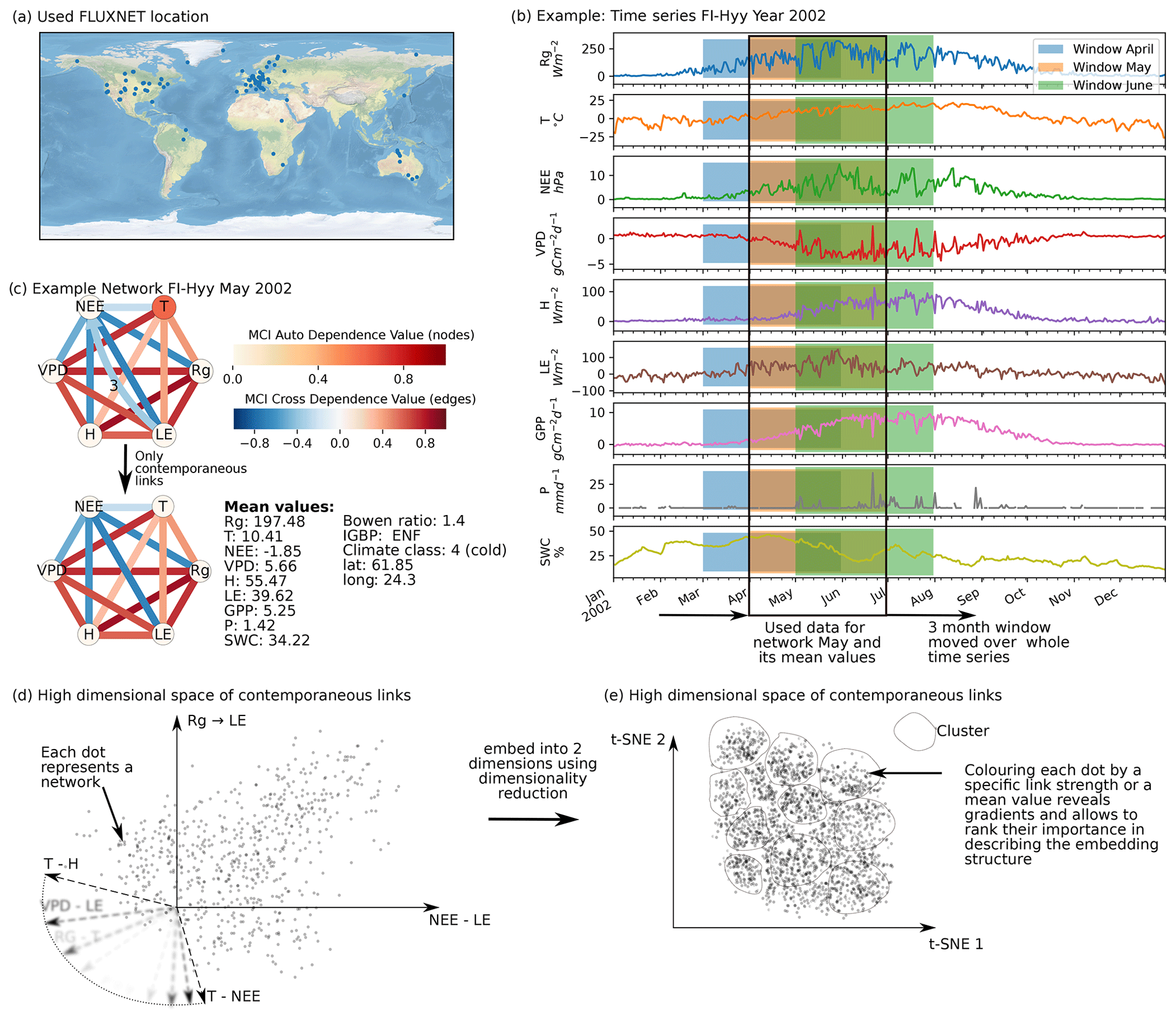
Figure 1Schematic representation of the workflow. (a) Eddy covariance data from the FLUXNET database are selected (119 sites). (b) For each site we used the time series of global radiation Rg, air temperature T, vapour pressure deficit VPD, net ecosystem exchange NEE, sensible heat H, latent heat LE, gross primary productivity GPP, precipitation P, and soil water content SWC. Networks are estimated in 3-month moving windows using Rg, T, NEE, VPD, LE, and H. (c) An example interaction network for FI-Hyy (Hyytiälä) in May 2002. Contemporaneous links are given by straight (undirected) edges; lagged links are given by curved arrows with a number indicating the time lag. The strongest and most persistent links are contemporaneous. Thus we limit our analysis to those links. (d) Each 3-month network can be interpreted as an observation in a 15-dimensional space (each contemporaneous link is one dimension). (e) Dimensionality reduction projects all interaction networks into a two-dimensional space preserving its local-neighbourhood structure. Here any subsequent analysis and interpretation will be realised.
2.8 Workflow
Our restrictions on the data length and quality resulted in a selection of 119 FLUXNET sites (Fig. 1a). Applying the above-described procedure we obtained 10 038 networks for the different months and sites. An example network estimated by PCMCI is shown in Fig. 1c. The strongest and most consistent links are contemporaneous, indicating that interactions happen on timescales shorter than the time resolution. While lagged common drivers are excluded, contemporaneous links can still be spurious due to contemporaneous confounding (see Sect. 2.2). Nevertheless, we focus our analysis on these 15 links, as they contain most information. This is done by performing the dimensionality reduction on contemporaneous links and neglecting the lagged ones. The rationale of employing a dimensionality reduction is the following. Each of the estimated networks constitutes one observation in a high-dimensional space with a network's links spanning its axes (Fig. 1d). Projecting this high-dimensional space onto two dimensions (Fig. 1e) allows first of all for visualisation. In the case that the data consist of a structure that can be “identified” by the dimensionality reduction method, the visualisation reveals the dominant features of transitions between different states of biosphere–atmosphere interactions. The dominant features are the links that appear with strong gradients in the low-dimensional embedding. To quantify and later rank the gradients exhibited by each link, we use the measure distance correlation (see Sect. 2.5). Therefore, we calculate the distance correlation of the link strengths (Fig. 1d) with their position on the low-dimensional embedding axes (Fig. 2d). We also examine the distance correlation of secondary quantities with the axes. The secondary quantities are firstly mean values of variables calculated for each 3-month period of network estimation as well as secondly static values like climate class, vegetation type, or location. The secondary quantities are used to find covariates of the low-dimensional embedding that can help to explain its structure. In a next step, we cluster the low-dimensional embedding to further understand to which network structures the gradients of link strength lead (see Sect. 2.4) and calculate the cluster's average networks (a simple mean). Up to this point (Sect. 3.1 and 3.2), we have analysed the manifold of biosphere–atmosphere interactions and can address the first part of our hypothesis. As each point of the low-dimensional embedding represents the biosphere–atmosphere interactions of a specific ecosystem at a specific time, we can investigate the behaviour of specific ecosystems (see Sect. 2.7). Therefore we look at the monthly median and annual trajectories of certain ecosystems (Sect. 3.3 and 3.4). This leads to the answer of the second part of our hypothesis.
3.1 Two-dimensional embedding of biosphere–atmosphere networks
To find the most suitable dimensionality reduction method, we evaluated three different methods (PCA, t-SNE, and UMAP) with respect to their ability to project the high-dimensional network space onto two dimensions. To compare the low-dimensional embedding spaces, we used the RNX(K) measure (see Sect. 2.4) which quantifies how well neighbourhoods are preserved when projecting the high-dimensional space onto fewer dimensions. We found that t-SNE achieved the best projection, by best preserving both local and distant neighbourhoods (cf. Sect. 2.4 and Figs. B1 and B2). This is unexpected, as UMAP is said to intentionally preserve the global structure. Yet, as can be seen in Fig. 4a, the networks almost form a continuum. Thus, by maintaining the local-neighbourhood structure, also the global structure is preserved within t-SNE.
The two-dimensional embedding by t-SNE of biosphere–atmosphere interactions is ordered primarily by dependencies including carbon flux (NEE) and energy distributions (LE and H). This can be seen in Fig. 2, which shows the Fig. 2d embedding colour-coded by the strength of individual links, i.e. MCI partial-correlation values. The colouring reveals that the link strengths are ordered along gradients; i.e. they exhibit some dependence with the t-SNE axes. Using distance correlation to rank those gradients (see Sect. 2.5), we find the links NEE–LE (ℛ=0.75), Rg–LE (ℛ=0.73), and T–H (ℛ=0.69) to have the strongest gradients. The connection between carbon and water fluxes as well as the role of energy input to sustain water fluxes (if available in the soil) are well-known and investigated dependencies (Beer et al., 2010; Luyssaert et al., 2007).
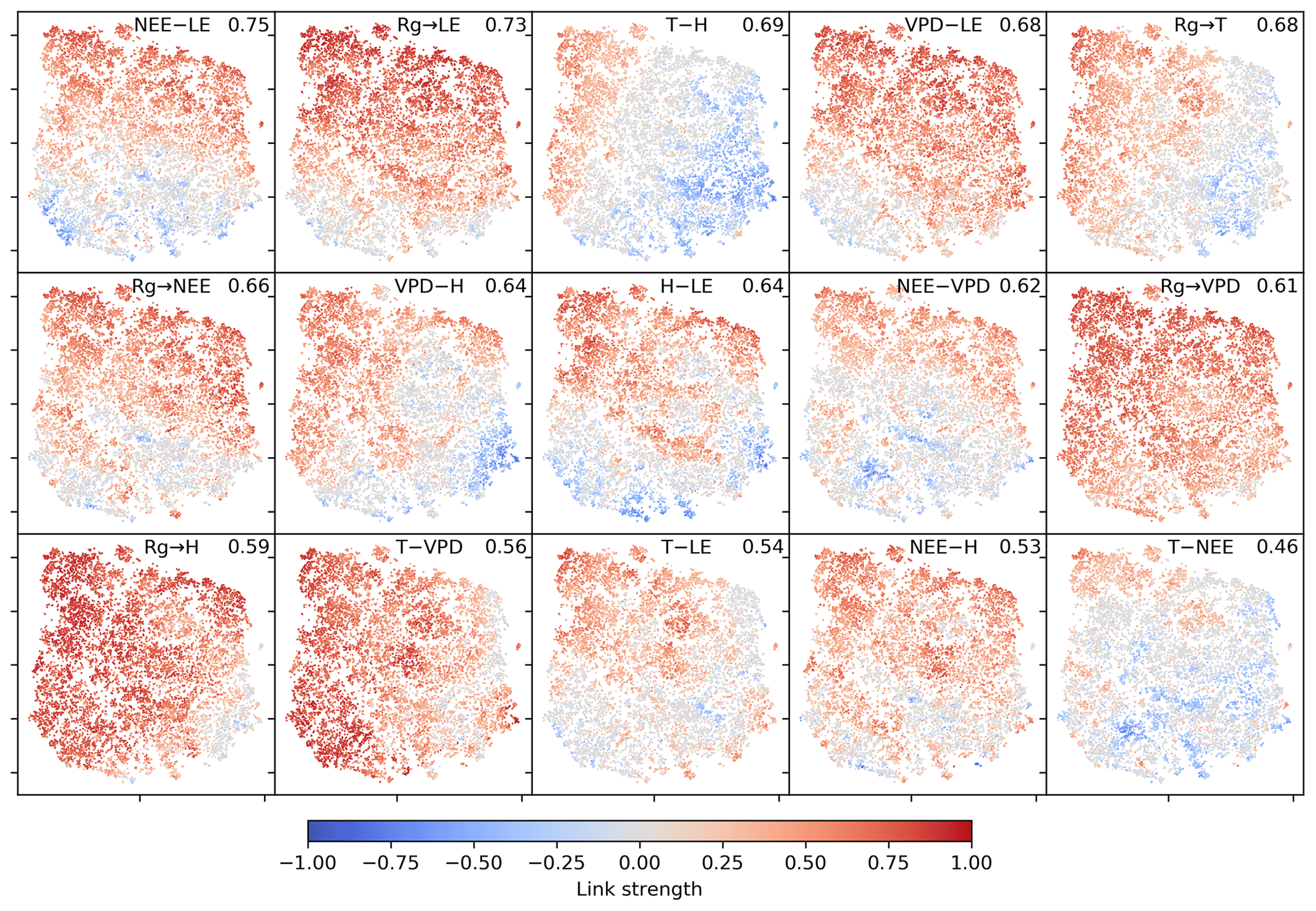
Figure 2Two-dimensional embedding of 3-monthly biosphere–atmosphere networks realised via t-SNE. Shown is the distribution of link strengths among the networks. The strength is estimated via MCI partial-correlation values. Panels are sorted by the distance correlation of the link's MCI value with the axes (value in the upper-right corner). As Rg is set as a potential driver (PCMCI parameter selected_links; see Table A2), connections including Rg are directed →. This setting does not affect the results (see Fig. B4).
To search for covariates that help to explain – and if thought further, help to predict the network structures – we colour-coded the embedding by the networks' underlying mean conditions, i.e. the average over the respective time window, of the exchange rates (GPP, NEE, LE, and H) as well as meteorological conditions (Rg, T, VPD, and P). This is shown in Fig. 3. Clearly, the mean exchange rates and meteorological conditions – although not considered in the estimation of the networks – are related to the observed biosphere–atmosphere interactions. On the contrary, corresponding vegetation types and Köppen-Geiger classes are not as much related as displayed in Fig. B6 in the Appendix . The results show that a high-dimensional space encompassing more than 10 000 ecosystem networks representing the states of biosphere–atmosphere interactions from ecosystems of various geographic origins can be reduced to a compact two-dimensional manifold characterised by four edges and gradients of mean biosphere and atmosphere conditions. While gradients in MCI partial-correlation strength are expected, as they were used as features in the dimensionality reduction, gradients in mean climatic and biospheric conditions were not. This information thus must be entailed in the networks' structure. To better grasp the distribution of network structures, we further analyse the emerging clusters.

Figure 3Two-dimensional embedding coloured by underlying mean exchange rates and meteorological conditions. The mean values are calculated over the respective time periods used for the network estimation. Each network is estimated on a 3-month window of daily time series data. Values are cut off at the highest and lowest percentile. Distance correlation of the shown quantity with the axes is given in the upper-right corner of each panel.
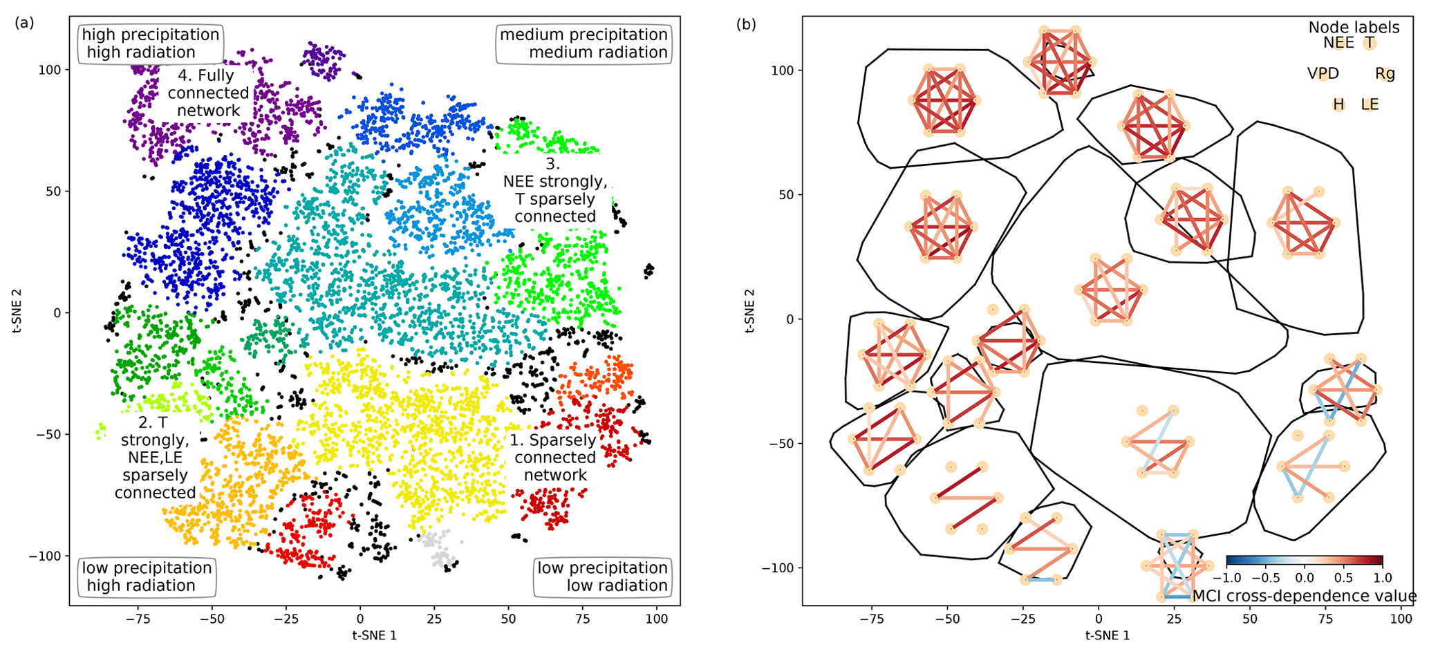
Figure 4Structure of the two-dimensional embedding. (a) t-SNE space clustered by the OPTICS approach (Ankerst et al., 1999). Colours represent different clusters; black dots are not attributed to a cluster. Indicated are the four archetypes of network connectivity and the networks' underlying meteorological conditions. (b) Convex hulls of clusters and their average network, i.e. average over all networks belonging to one cluster. Average networks are thresholded at a minimum link strength of 0.2. A finer clustering can be found in Fig. B5 in the Appendix.
3.2 Clusters of characteristic ecosystem–atmosphere networks
As we apply a significance threshold to each link of the estimated network structures (see Sect. 2.3), the networks typically lack weak links. This leads to a certain degree of clustering among the networks, which we identified using the OPTICS approach (see Sect. 2.6; Ankerst et al., 1999) (Fig. 4a). Cluster boundaries are shown by the convex hulls in Fig. 4b, where we also visualise the mean networks of each cluster. This visualisation reveals that the mean networks of the clusters situated at the embedding's edges can be regarded as archetypes of network structures, i.e. extremal, characteristic states (similar to the concept of endmember states). The four states can be described as follows:
-
Type 1 is a sparsely connected network. Links, if present, are very weak and predominantly exist among atmospheric variables. Mean atmospheric conditions are characterised by low energy input (low Rg and T). Carbon and water fluxes are consequently close to 0, and daily averages of sensible heat can even reach negative values. Such conditions reflect high-latitude ecosystem winter states experienced by ecosystems like the evergreen needleleaf forest (ENF) of Finland, i.e. Hyytiälä (FI-Hyy) and Sodankylä (FI-Sod), and Canada, i.e. the UCI-1850 burn site (CA-NS1) and the Quebec – Eastern Boreal (CA-Qcu) site during December and January.
-
Type 2 consists of strong links among atmospheric variables, but LE and NEE are weakly, not, or even negatively connected to the atmosphere, i.e. the meteorological variables. This network structure coincides with high energy input (high Rg and T) but low water availability (low P and SWC and high VPD). A high Bowen ratio, i.e. the ratio between sensible heat and latent heat, representing aridity, and low absolute carbon fluxes (GPP and NEE) are the consequence. These conditions are typically present at semi-arid ecosystems like the woody-savanna (WSA) Santa Rita Mesquite (US-SRM) as well as the grassland Santa Rita (US-SRG) sites, Audubon Research Ranch (US-Aud), and Sturt Plains (AU-Stp) during the dry season.
-
Type 3 exhibits the same strong links among Rg, VPD, and H as Type 2, but T is weakly or not connected. The opposite is true for links of LE and NEE, which are strongly connected to the other variables (except T). Rg and T are considerably lower than in Type 2 (approximately by 100 W m−2 and 10 ∘C), but because of sufficient water availability the Bowen ratio is between 0 and 1. Typical ecosystems in this state are mid- to high-latitude forests during spring or autumn, e.g. Harvard Forest EMS Tower (US-Ha1, deciduous broadleaf forest (DBF)), Roccarespampani 1 (IT-Ro1, DBF), Vielsalm (BE-Vie, mixed forest (MF)), and Hyytiälä (FI-Hyy, ENF).
-
Type 4 is fully and strongly connected. Both energy input and water availability are high, leading to Bowen ratios around 1. This network state is typically present in tropical forests like the Guyaflux site in French Guiana (GF-Guy) (evergreen broadleaf forest (EBF)) but can temporarily be also reached by a variety of other ecosystems, e.g. mid- and high-latitude forests like Hainich (DE-Hai, DBF), Tharandt (DE-Tha, ENF), BE-Vie (MF), and FI-Hyy (ENF) as well as woody savanna (WSA) such as Howard Springs (AU-How) and grassland (GRA) such as Daly River Savanna (AU-Dap).
The archetypes of networks are located at the edges of the two-dimensional space and thus could define two imaginary axes. From a physical point of view, energy is required for each process and interaction to occur, e.g. photosynthesis or evaporation (Bonan, 2015). Therefore, transitions along the axis connecting the network types 1 and 4 might be interpreted as energy controlled, as dependencies among all variables fade or increase consistently. Transitions along the axis connecting network types 2 and 3 are explainable by a combination of water availability and a temperature gradient. Low water availability but high temperatures cause a shutdown of stomatal conductance or ecosystems to enter a dormant state, which leads to low carbon and water fluxes and low connectivity. On the other hand, sufficient water and medium temperatures (around the optimum of photosynthesis) allow for carbon and water fluxes but reduce the influence of varying temperatures, leading to connected NEE and LE but disconnected T. And indeed these patterns and gradients exist. Mean Rg is lowest at network type 1 and almost linearly increases towards network type 4. P is lowest at network types 1 and 2. In combination with high energy input network type 2 has the lowest SWC values and the highest Bowen ratios (see Appendix Fig. B6). SWC is higher but quite dispersed elsewhere, suggesting that at a certain point water limitations are fading out. T values of course also show an increase not only from network types 1 to 4 (as radiation) but also from network types 3 to 2 and are actually rather low (8 to 15 ∘C) at network type 3 (see Fig. 3). As meteorological conditions affect biosphere productivity, network types 1 and 2 exhibit low, type 3 medium, and type 4 high productivity, i.e. estimated as GPP. In short, the clustering revealed that changes in energy and water availability can explain major transitions between different states of biosphere–atmosphere interactions. This is in line with a recent study showing that a variety of land-surface processes can be largely summarised by on the one hand productivity measures and on the other hand water and energy availability. Both water and energy availability need to be high for highly productive states, yet the lack of either of them leads to low productivity (Kraemer et al., 2020a). This biosphere state triangle is found in our analysis by the network types 1 (cold – low connectivity), 2 (dry – NEE/LE weakly connected), and 4 (high productivity – fully connected). Yet, a fourth network type (type 3) is naturally occurring in the t-SNE space, as we here include interactions with the atmosphere.
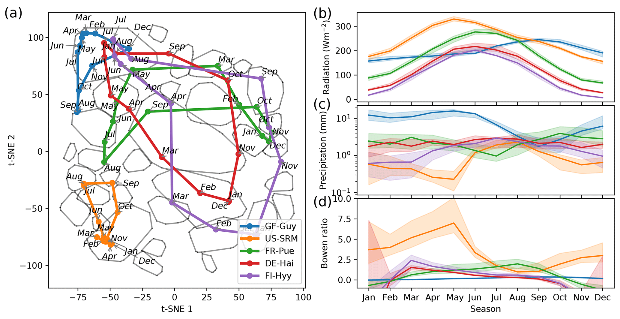
Figure 5Median trajectories of selected sites (a) and their corresponding mean values of radiation, precipitation, and the Bowen ratio (b). In winter months the Bowen ratio can turn negative. Nevertheless we set the lower limit of the y axis to 0. As networks are calculated using a centred 3-month moving window, each month is ascribed to a network. Thus, the behaviour of an ecosystem can be tracked by its monthly networks, which form trajectories for each year. An ecosystem's monthly median trajectory is composed of the two-dimensional monthly median networks (see Sect. 2.7 for details).
Up to this point we have found strong evidence supporting our first hypothesis. The manifold of biosphere–atmosphere interactions can be represented rather well by two dimensions, which we identified to be most consistent with energy and water availabilities. It is confined by four characteristic states and populated homogeneously by the observed network states. Having an understanding of the low-dimensional embedding's structure now allows us to analyse specific ecosystem behaviour.
3.3 Ecosystems' median trajectories
Each point in the reduced t-SNE space represents a biosphere–atmosphere interaction network for a given month and ecosystem. Hence, we can trace an ecosystem's trajectory through time. We are first focusing on an ecosystem's median monthly trajectory (see Sect. 2.7) within the low-dimensional space. We can see that the median trajectories reflect seasonal patterns of meteorological conditions (Fig. 5). For example, mid-latitude sites like FR-Pue (Puechabon, EBF), DE-Hai (DBF), and FI-Hyy (ENF) exhibit a strong seasonal variation of Rg and span a long distance in the t-SNE space. In contrast, tropical ecosystems like GF-Guy (EBF) constantly have high Rg and exhibit predominantly network type 4, indicative of highly productive conditions, while DE-Hai or FI-Hyy reach this connectivity pattern only during peak growing season. US-SRM (WSA), however, has similar or even higher Rg values throughout the year but barely manages to deviate from type 2, which is in accordance with its low water availability. The amount of precipitation further aligns with differences and characteristics of the trajectories of FR-Pue, DE-Hai, and FI-Hyy. For example, FI-Hyy shows some deviation towards edge 2 in February and March, as does FR-Pue in June, July, and August. For both, mean precipitation is lowest during these months. These behaviours demonstrate what the previous figures (Figs. 3 and 4) have already suggested: ecosystems populate the low-dimensional space and migrate within as allowed by their climatic conditions. Thereby they can exhibit a wide range of interaction structures as can be seen from the mid-latitude sites. As these behaviours are multi-year averages, they could resemble more ecosystem adaptation to median climatic conditions than flexible adjustment of biosphere–atmosphere interactions to quickly changing meteorological conditions. If biosphere–atmosphere interactions are confined by adaptation shall be investigated in the final analysis section.
3.4 Deviations from ecosystem median trajectories
The remaining open question is how flexibly do the networks adjust to deviations from mean climatic conditions. Therefore, we look at climatic anomalies. Figure 6 shows the trajectories of ecosystems during anomalous dry or wet conditions. During the European heatwave of 2003, in July and August the trajectories of two temperate central European forests, DE-Hai and DE-Tha, no longer manage to establish a network structure resembling network type 4, typical for these ecosystems during their highly productive phase. Instead they are shifted towards network type 2, associated with drier conditions (Fig. 6a and b). Similarly, the ecosystem BR-Sa3 (EBF) in the Brazilian tropical rainforest shows substantial deviations towards network type 2 during the exceptional dry season of 2001 (August, September, and October) (Marengo et al., 2018) (Fig. 6c). In contrast, US-Wkg (Walnut Gulch Kendall Grasslands) is a grassland accustomed to dry conditions and thus predominantly exhibits low water and carbon fluxes resulting in network structures like those of network type 2; i.e. water and carbon fluxes are barely or even not connected. Carbon and water fluxes of semi-arid ecosystems, however, are known to respond quickly and strongly to sufficient precipitation (Potts et al., 2019; Leon et al., 2014; Reynolds et al., 2004). This sensitivity is found to carry over to the network structure as well. The network structure of US-Wkg becomes fully connected (network type 4) in September 2014 with above-average precipitation (NOAA, 2015) (Fig. 6d). In summary, climatic extremes are visible in an ecosystem's trajectory as strong deviations from the median trajectory. With this finding we have to reject our second hypothesis that owing to an ecosystem's adaptation its accessible functional states are limited to a certain range. The opposite seems to be valid. Biosphere–atmosphere interactions can flexibly follow atmospheric conditions and are not confined to certain states.
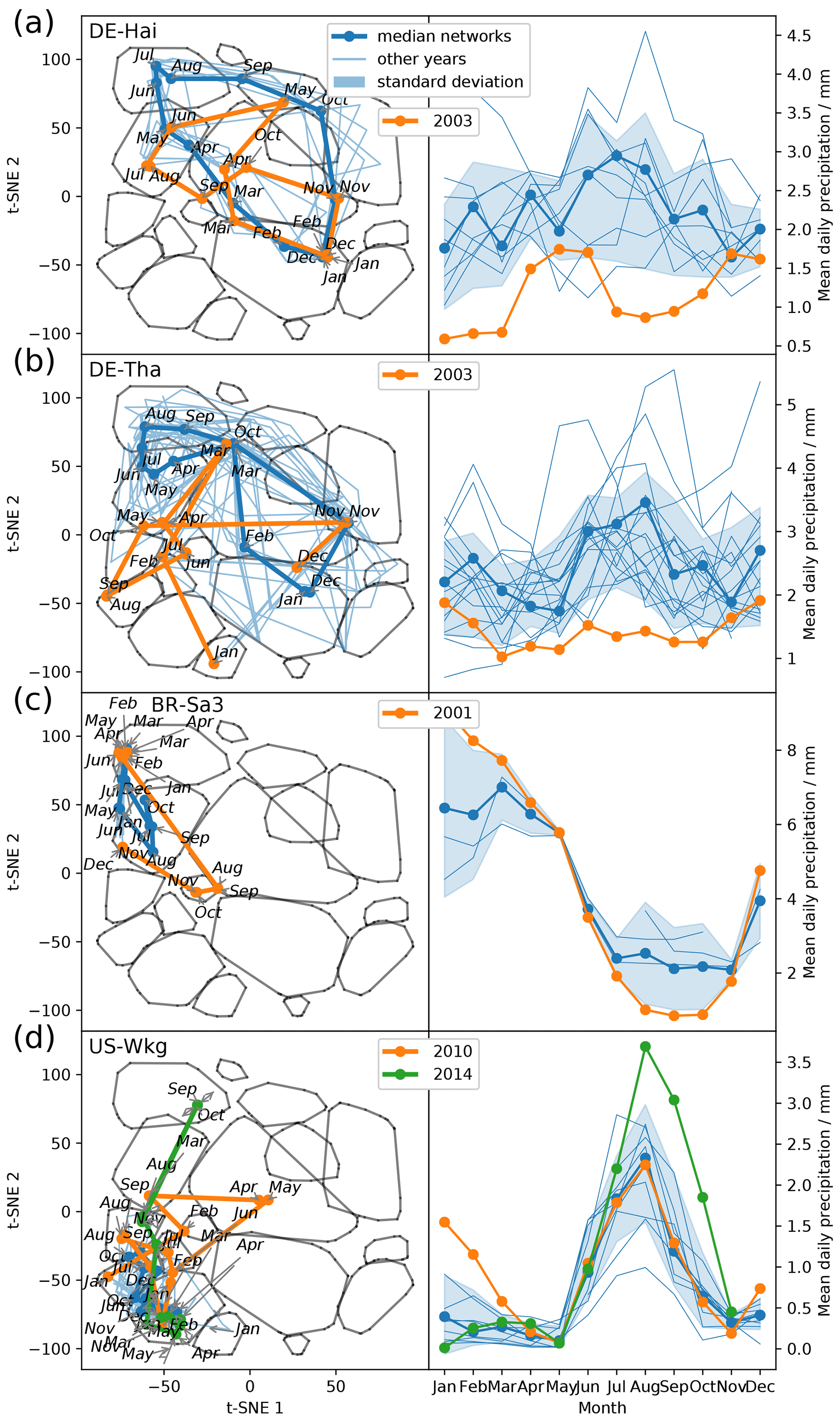
Figure 6Abnormal conditions in meteorological conditions (here precipitation) become visible in an ecosystem's trajectory. (a) Trajectories within the low-dimensional space of the ecosystems Hainich (DE-Hai, DBF), Tharandt (DE-Tha, ENF), Santarem-Km83-Logged Forest (BR-Sa3, EBF), and Walnut Gulch Kendall Grasslands (US-Wkg, GRA); (b) 3-monthly average of daily precipitation data.
3.5 Functional convergence of biosphere–atmosphere interactions
We have seen that networks representing biosphere–atmosphere interactions strongly align with prevailing mean meteorological conditions. Moreover, the visualisation of ecosystem trajectories within the t-SNE space (Figs. 5 and 6) and the distributions of vegetation types and climatic regions (Appendix Fig. B6) reveal that ecosystems across vegetation types and climatic regions can exhibit similar biosphere–atmosphere interactions if their meteorological conditions are similar. For example, we found a fully connected network (type 4) to be associated with high radiation and water availability and thus optimal growing conditions, which results in high carbon and water fluxes. Diverging from optimal growing conditions, links in the networks weaken and disappear. This behaviour can be understood as the functional convergence of ecosystems, which corroborates the hypothesis that ecosystems have a low number of key processes that determine ecosystem behaviour (Lambert, 2006; Meinzer, 2003; Shaver et al., 2007), rendering their behaviour transparent and predictable.
Criticism might rise, as the larger part of the biosphere–atmosphere interaction network indeed is a pure atmospheric network, i.e. Rg, T, VPD, and H. Thus strong associations of networks and their trajectories with atmospheric conditions could be dominated by changes in this atmospheric network. Figure 2, however, suggests the opposite. The strongest gradients are given by the links NEE–LE and Rg–LE, and transitions along the axis connecting types 2 and 3 (cf. Fig. 4) are dominated by changes in biosphere connectivity, i.e. LE and NEE.
In fact, the dominance of climatic drivers in controlling the temporal evolution of ecosystem functioning emerges also in other studies (Musavi et al., 2017; Schwalm et al., 2017; Kraemer et al., 2020a), as they showed that carbon fluxes are primarily controlled by climatic factors. Yet, these and others also show the role of biotic factors in shaping the responses of ecosystem processes to climatic variability. For example, Musavi et al. (2017) revealed in a global ecosystem study that species diversity and ecosystem age decrease interannual variability of GPP. Similarly, Wagg et al. (2017) showed biodiversity to increase long-term stability of ecosystem productivity. In regional studies Wales et al. (2020) found the stability of net primary production to be affected by the kind and severity of disturbances. Tamrakar et al. (2018) showed that seasonal carbon fluxes were more sensitive to environmental conditions in a homogeneous forest compared to a heterogeneous one. It would be of interest to investigate to which degree the effects of biotic factors also translates to the sensitivity of the network structure.
Furthermore, extreme heat and drought events (Sippel et al., 2018) or compound events in general (Zscheischler et al., 2020) can severely disrupt ecosystem functions. The time of recovery from such disturbances is a crucial parameter in assessing ecosystem resilience. Schwalm et al. (2017) showed that the recovery time measured, as the recovery in GPP is primarily influenced by climate but secondarily by biodiversity and CO2 fertilisation. Assessing the recovery time via GPP already puts the ecosystem functioning into focus. The presented framework here, i.e. the sensitivity of an ecosystem's network structure to meteorological conditions, might be a valuable asset in studying reaction time and strength to and recovery from extreme events, as it not only utilises one variable but also the interactions of a set of variables, thereby capturing more comprehensively an ecosystem state. A drawback is the reduced temporal resolution (a certain time period of daily or even half-hourly measurements is aggregated to one network), which can be offset by the moving window approach used here to a certain degree. Especially with regard to climatic extreme conditions in recent years with observed vegetation dieback in, for example, DE-Hai (Schuldt et al., 2020), further studies could also shed light on the role of adaptation in shaping biosphere–atmosphere interactions. Our study suggests that adaptation to a lesser degree limits the range of possible interactions but enables sustaining and persisting certain conditions for longer periods. The focus of further studies thus could be to elucidate the role of biotic factors in influencing ecosystem trajectories as well as the role of adaptation and the response to extreme events.
3.6 Limitations of the study
Finally, we would like to take a critical view on our analysis approach. As stated in Sect. 2.2, PCMCI might fail to identify some spurious links due to the occurrence of contemporaneous confounders. Thus networks can not be interpreted causally, but this does not severely hinder their value for the current analysis. In addition we include a rather limited set of variables into the network estimation. Thus we cannot and do not claim that ecosystems become fully alike under similar meteorological conditions. Yet, on the timescale investigated the data show that the interactions among the chosen set of variables can be described by very similar structures. Follow-up studies might search for and include further biosphere variables. Currently, an analysis of the biotic effects on the network structure is hampered because the t-SNE space is not metric. Thus, for instance, the effect of a drought with a similar magnitude in a boreal and temperate forest cannot simply be compared by the deviation from their median trajectory.
We analysed the functional behaviour of a variety of ecosystems using the FLUXNET database of carbon, water, and energy flux measurements. In particular, we examined the interaction structure between biosphere–atmosphere fluxes as well as atmospheric state variables using PCMCI, a method to estimate causal relationships from empirical time series under certain assumptions. Using non-linear dimensionality reduction, we find evidence supporting our hypothesis that the manifold of existing states is bound by few, i.e. four, archetypes of network states. They are characterised on the one hand by a fully connected and almost unconnected network structure and on the other hand by an antagonistic coupling of carbon and water flux with temperature – when one is strongly coupled, the other is decoupled. The transitions between these states correlate well with gradients of meteorological drivers, i.e. radiation and water availability. The movement of an ecosystem within that space therefore strongly aligns with changes in meteorological conditions. This, however, also leads to similar behaviour under similar conditions for strongly contrasting ecosystems. For example, forests of mid or even high latitudes exhibit an interaction structure similar to tropical forests given high radiation and water availability during summer. Yet, this state can also be reached by predominantly dry ecosystems like steppe grasslands given sufficient precipitation. In contrast if productive ecosystems are struck by a severe drought, like central European ecosystems in 2003, the behaviour can adapt more to that of a Mediterranean ecosystem. Thus the second part of our hypothesis must be rejected. The analysis shows that the biosphere–atmosphere interaction structure can adapt flexibly to prevailing conditions and is widely independent of vegetation type and climatic region. Such behaviour is strong evidence for functional convergence of ecosystems; i.e. their behaviour is determined by a low number of key processes. For further studies, we suggest focusing on the role of biotic factors such as, for example, plant functional types, ecosystem age, and adaptation. These factors could play a crucial role in understanding the ecosystem coping strategies to climatic extremes.
Table A1List of FLUXNET sites used for the generation of artificial datasets and the time period used. IGBP: International Geosphere–Biosphere Programme. DBF: deciduous broadleaf forest; OSH: open shrubland; WET: wetland; CRO: cropland; CSH: closed shrubland; MF: mixed forest; EBF: evergreen broadleaf forest; WSA: woody savanna; SAV: savanna; ENF: evergreen needleleaf forest; GRA: grassland.
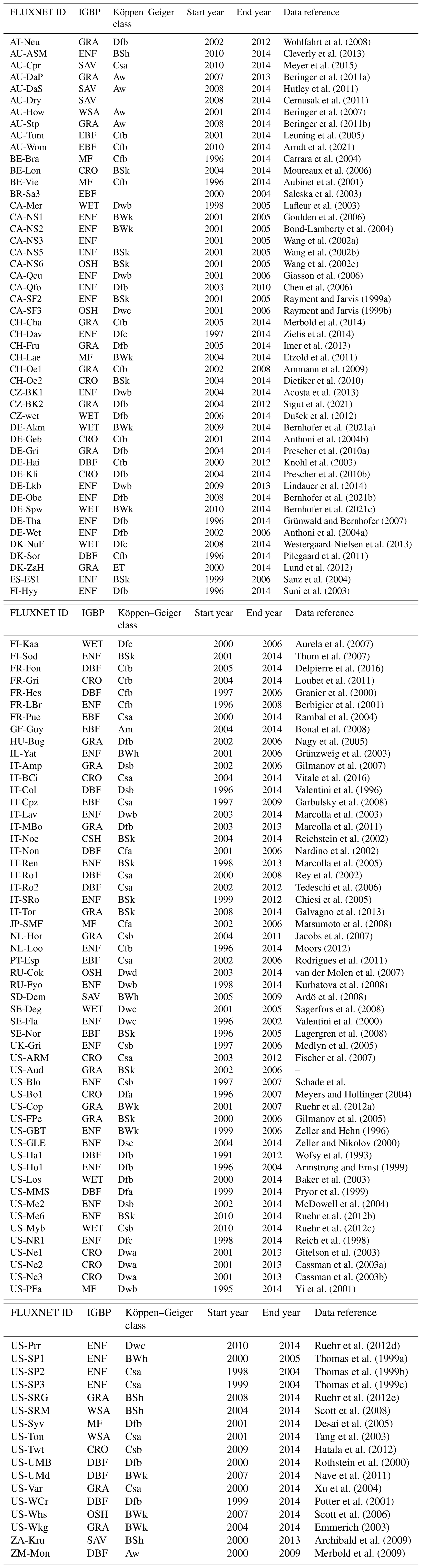
Table A2PCMCI parameters that were used differently from default settings.
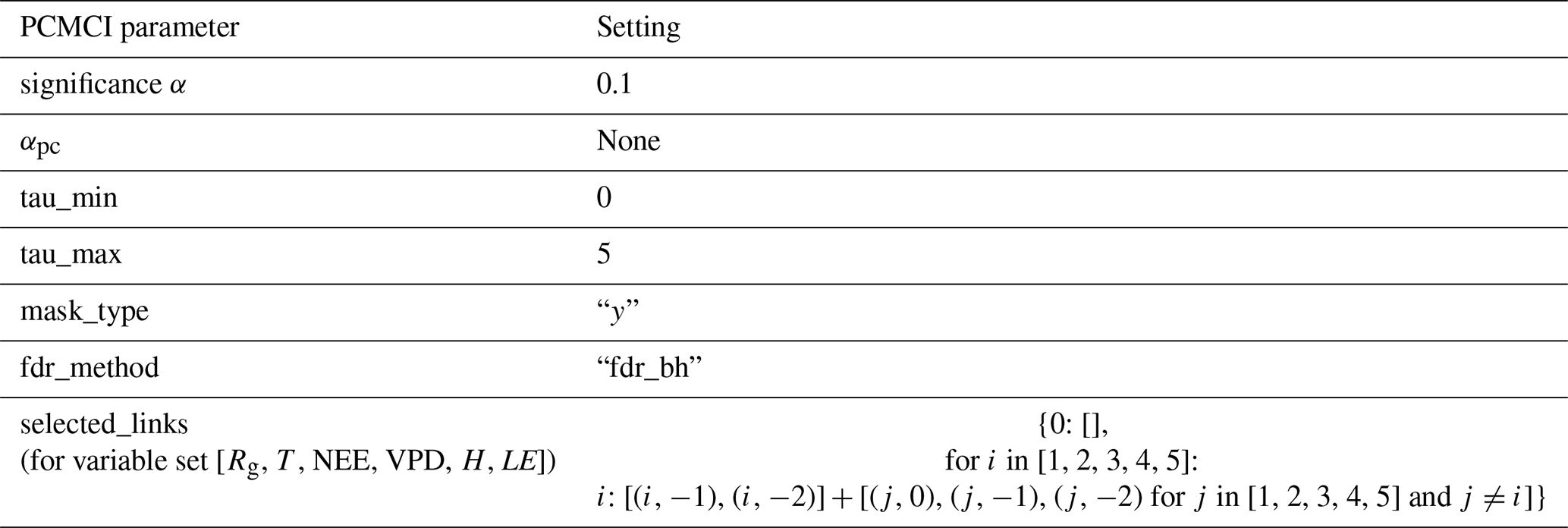
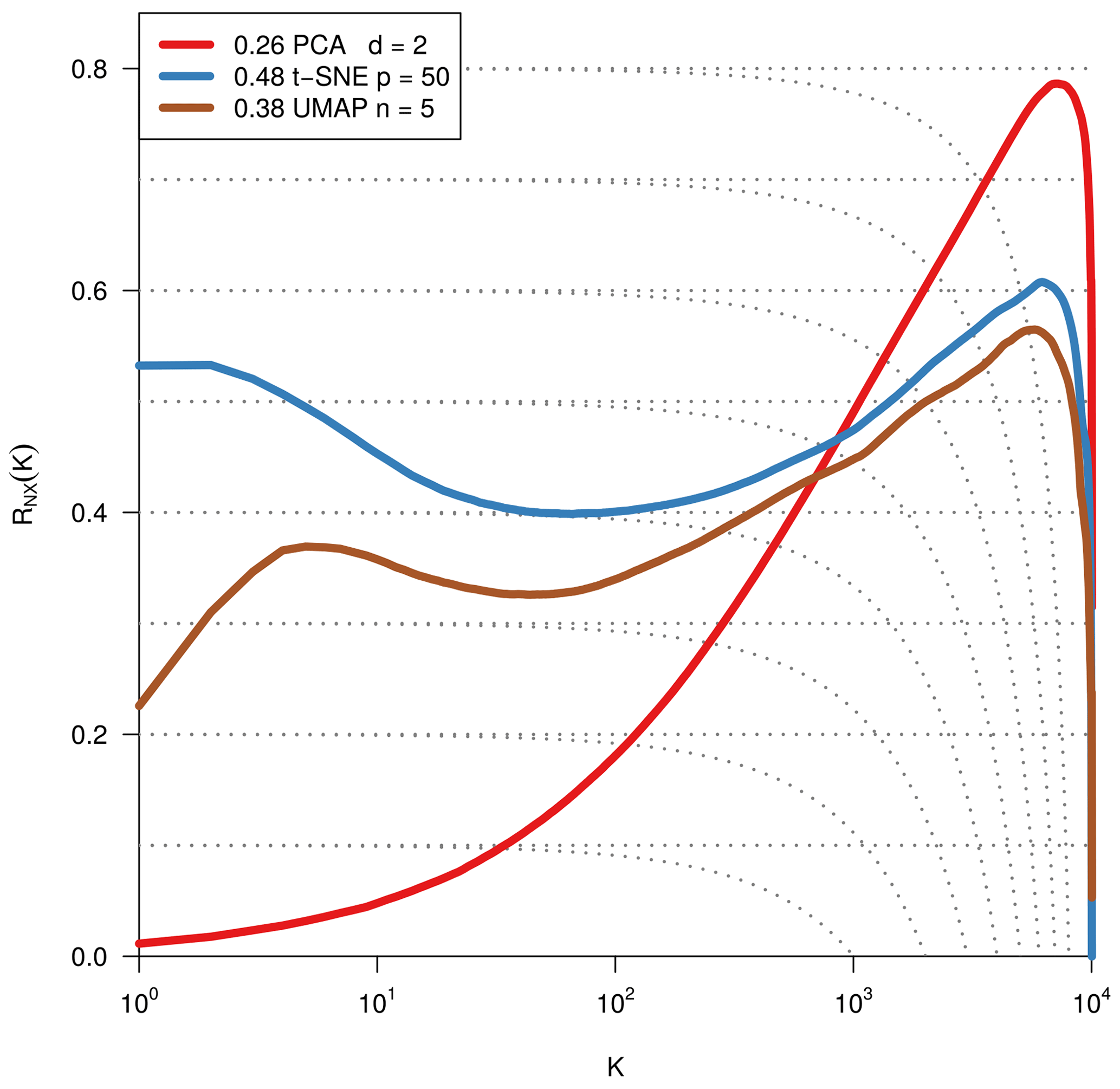
Figure B1Quality assessment of dimensionality reduction techniques. To visualise and subsequently analyse the network space, we reduce its dimensionality. We compared PCA, t-SNE, and UMAP including various parameter settings (here: PCA's leading two principal components, t-SNE with perplexity 30 and UMAP with nneighbours equal to 5 for two dimensions). The test statistic RNX(k) (y axis) gives the improvement of the embedding of K-ary neighbourhoods (x axis) over a random embedding. The area under the curves (preserving the log-scaled x axis) is given in the legend and gives an idea of the overall quality of the embedding (Lee et al., 2015). We chose t-SNE with perplexity 30, as it preserves best local neighbourhoods and performs well on larger distances.
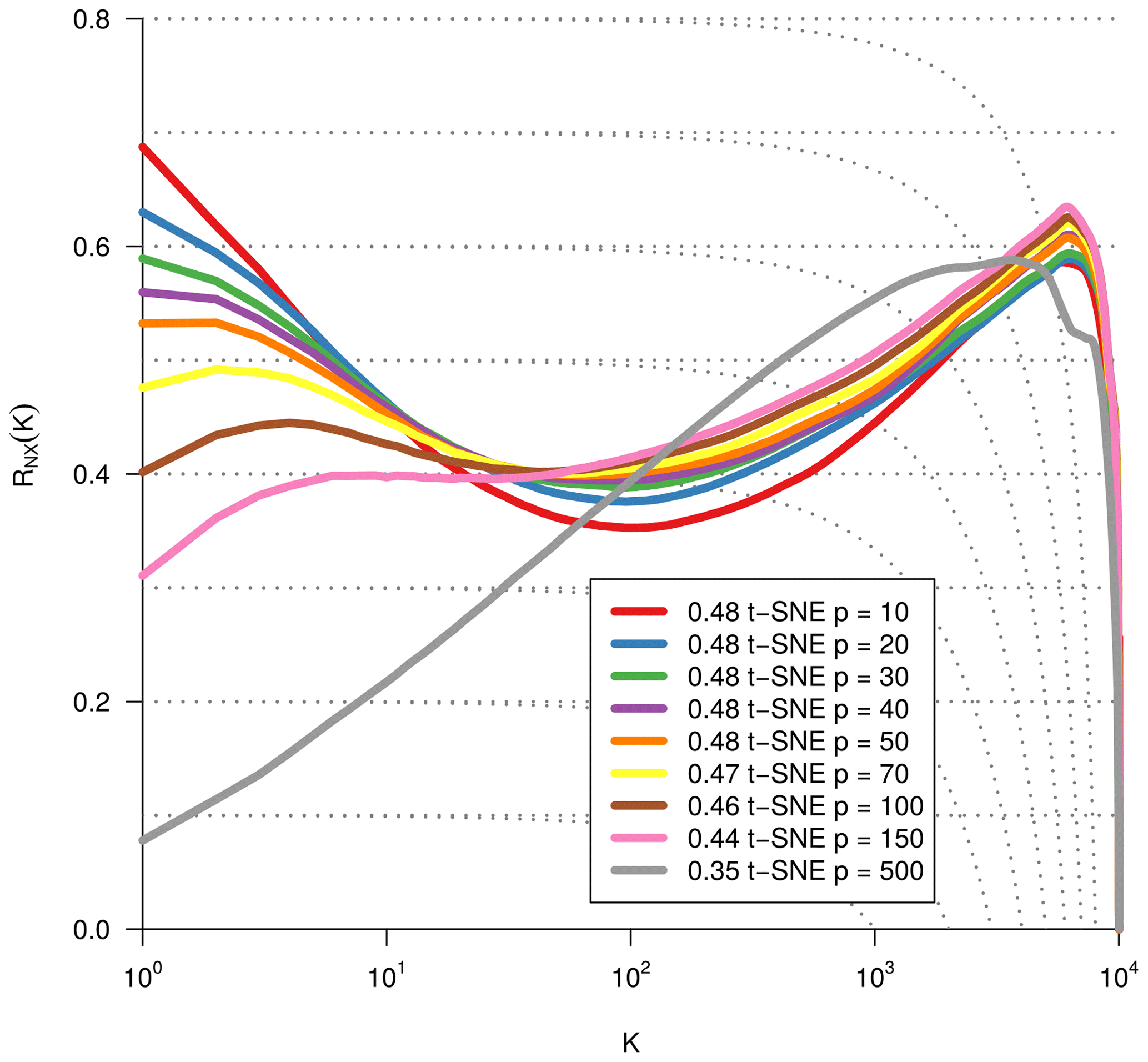
Figure B2Same metric as Fig. B1. Optimisation of the dimensionality reduction via t-SNE by using different perplexity values.
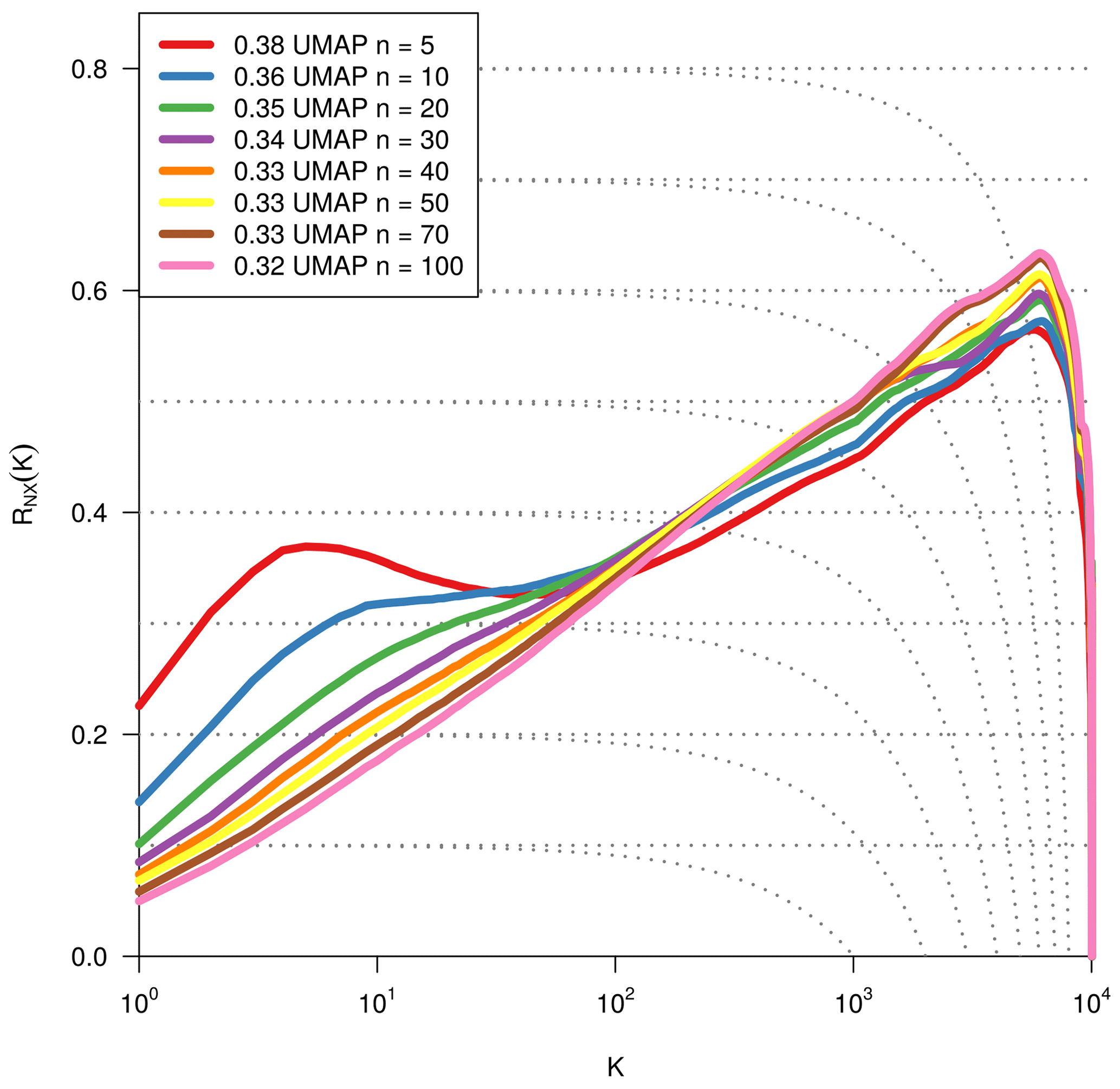
Figure B3Same metric as Fig. B1. Optimisation of the dimensionality reduction to two dimensions via UMAP by using different values for the parameter nneighbours.

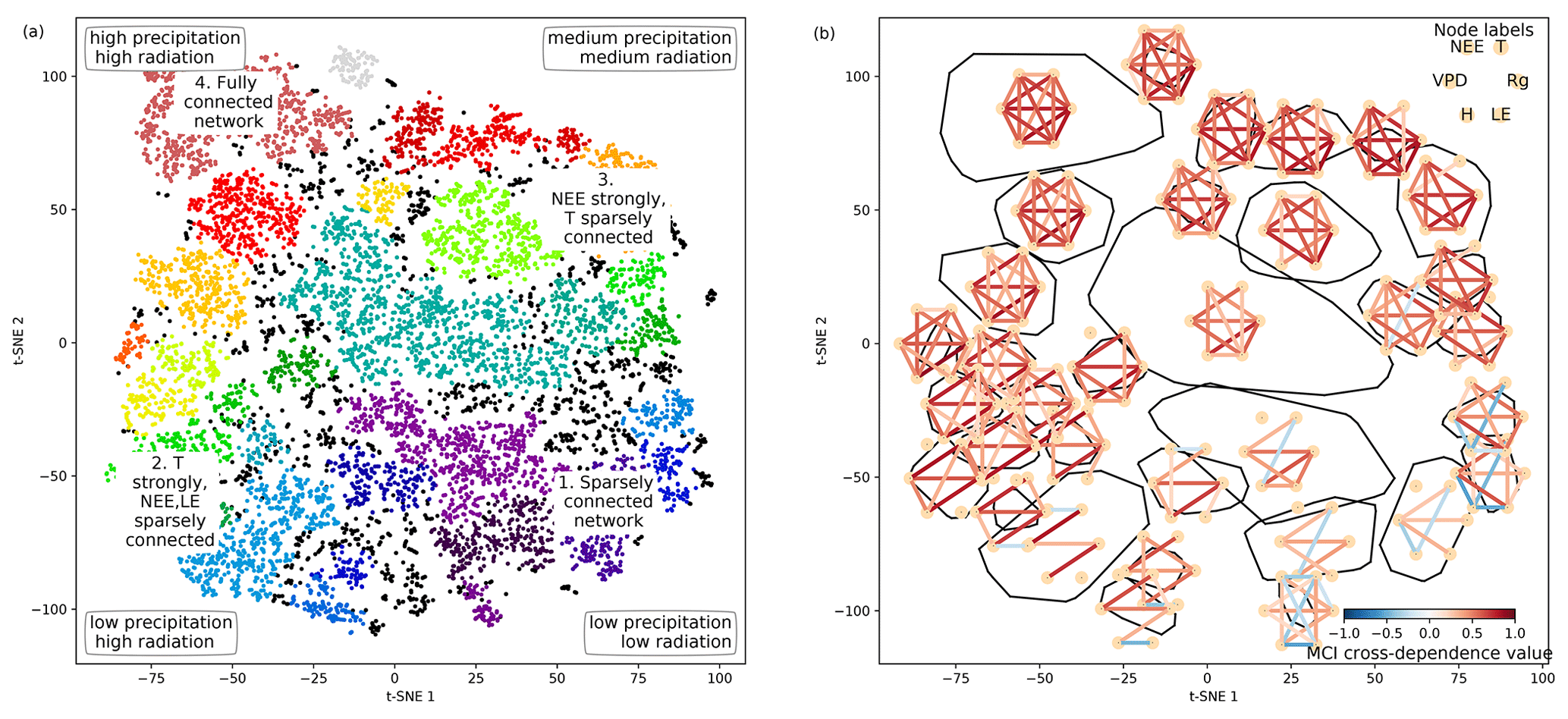
Figure B5Same as Fig. 4 but with smaller clusters exhibiting the finer structure of the t-SNE space.

Figure B6t-SNE space coloured by the underlying mean Bowen ratio and precipitation, as well as the ecosystem's respective Köppen–Geiger class and IGBP type.
Code scripts can be found at https://github.com/ckrich/Functional (Krich, 2021).
The eddy covariance data of the FLUXNET sites can be downloaded from the official web page (http://fluxnet.fluxdata.org/, last access: 14 April 2021).
CK and MDM designed the study with contributions from all other authors. CK conducted the analysis and wrote the manuscript. All authors helped to improve the manuscript.
The authors declare that they have no competing financial interests.
Diego G. Miralles acknowledges support from the European Research Council (DRY-2-DRY; grant agreement no. 715254). Christopher Krich thanks the Max Planck Research School for Global Biogeochemical Cycles for supporting his PhD project as well as Jacob A. Nelson in helping to assemble the dataset. This work used eddy covariance data acquired and shared by the FLUXNET community, including the following networks: AmeriFlux, AfriFlux, AsiaFlux, CarboAfrica, CarboEuropeIP, CarboItaly, CarboMont, ChinaFlux, Fluxnet-Canada, GreenGrass, ICOS, KoFlux, LBA, NECC, OzFlux-TERN, TCOS-Siberia, and USCCC. The ERA-Interim reanalysis data are provided by ECMWF and processed by LSCE. The FLUXNET eddy covariance data processing and harmonisation were carried out by the European Fluxes Database Cluster, AmeriFlux Management Project, and FluxData project of FLUXNET, with the support of CDIAC; ICOS Ecosystem Thematic Centre; and the OzFlux, ChinaFlux, and AsiaFlux offices.
The article processing charges for this open-access publication were covered by the Max Planck Society.
This paper was edited by Alexandra Konings and reviewed by three anonymous referees.
Acosta, M., Pavelka, M., Montagnani, L., Kutsch, W., Lindroth, A., Juszczak, R., and Janouš, D.: Soil Surface CO2 Efflux Measurements in Norway Spruce Forests: Comparison between Four Different Sites across Europe – from Boreal to Alpine Forest, Geoderma, 192, 295–303, https://doi.org/10.1016/j.geoderma.2012.08.027, 2013. a
Ammann, C., Spirig, C., Leifeld, J., and Neftel, A.: Assessment of the Nitrogen and Carbon Budget of Two Managed Temperate Grassland Fields, Agr. Ecosys. Environ., 133, 150–162, https://doi.org/10.1016/j.agee.2009.05.006, 2009. a
Ankerst, M., Breunig, M. M., Kriegel, H.-P., and Sander, J.: OPTICS: ordering points to identify the clustering structure, ACM Sigmod record, 28, 49–60, 1999. a, b, c
Anthoni, P., Knohl, A., Rebmann, C., Freibauer, A., Mund, M., Ziegler, W., Kolle, O., and Schulze, E.-D.: Forest and agricultural land-use-dependent CO2 exchange in Thuringia, Germany, Glob. Change Biol., 10, 2005–2019, 2004a. a
Anthoni, P. M., Knohl, A., Rebmann, C., Freibauer, A., Mund, M., Ziegler, W., Kolle, O., and Schulze, E.-D.: Forest and Agricultural Land-Use-Dependent CO2 Exchange in Thuringia, Germany, Glob. Change Biol., 10, 2005–2019, https://doi.org/10.1111/j.1365-2486.2004.00863.x, 2004b. a
Archibald, S. A., Kirton, A., van der Merwe, M. R., Scholes, R. J., Williams, C. A., and Hanan, N.: Drivers of Inter-Annual Variability in Net Ecosystem Exchange in a Semi-Arid Savanna Ecosystem, South Africa, Biogeosciences, 6, 251–266, https://doi.org/10.5194/bg-6-251-2009, 2009. a
Ardö, J., Mölder, M., El-Tahir, B. A., and Elkhidir, H. A. M.: Seasonal Variation of Carbon Fluxes in a Sparse Savanna in Semi Arid Sudan, Carbon Balance and Management, 3, 7, https://doi.org/10.1186/1750-0680-3-7, 2008. a
Armstrong, N. and Ernst, E.: The treatment of eczema with Chinese herbs: a systematic review of randomized clinical trials, Brit. J. Clin. Pharmaco., 48, 262, https://doi.org/10.4141/cjss93-034, 1999. a
Arndt, S., Hinko-Najera, N., Griebel, A., Beringer, J., and Livesley, S. J.: FLUXNET2015 AU-Wom Wombat, https://doi.org/10.18140/FLX/1440207, 2021. a
Aubinet, M., Chermanne, B., Vandenhaute, M., Longdoz, B., Yernaux, M., and Laitat, E.: Long Term Carbon Dioxide Exchange above a Mixed Forest in the Belgian Ardennes, Agr. Forest Meteorol., 108, 293–315, https://doi.org/10.1016/S0168-1923(01)00244-1, 2001. a
Aubinet, M., Vesala, T., and Papale, D.: Eddy covariance: a practical guide to measurement and data analysis, Springer Science & Business Media, 2012. a
Aurela, M., Riutta, T., Laurila, T., Tuovinen, J.-P., Vesala, T., Tuittila, E.-S., Rinne, J., Haapanala, S., and Laine, J.: CO2 exchange of a sedge fen in southern Finland-The impact of a drought period, Tellus B, 59, 826–837, 2007. a
Baker, I., Denning, A. S., Hanan, N., Prihodko, L., Uliasz, M., Vidale, P.-L., Davis, K., and Bakwin, P.: Simulated and Observed Fluxes of Sensible and Latent Heat and CO2 at the WLEF-TV Tower Using SiB2.5, Glob. Change Biol., 9, 1262–1277, https://doi.org/10.1046/j.1365-2486.2003.00671.x, 2003. a
Baldocchi, D.: “Breathing” of the terrestrial biosphere: lessons learned from a global network of carbon dioxide flux measurement systems, Austr. J. Bot., 56, 1–26, 2008. a
Baldocchi, D.: Measuring fluxes of trace gases and energy between ecosystems and the atmosphere – the state and future of the eddy covariance method, Glob. Change Biol., 20, 3600–3609, https://doi.org/10.1111/gcb.12649, 2014. a
Baldocchi, D., Falge, E., Gu, L., Olson, R., Hollinger, D., Running, S., Anthoni, P., Bernhofer, C., Davis, K., Evans, R., Fuentes, J., Goldstein, A., Katul, G., Law, B., Lee, X., Malhi, Y., Meyers, T., Munger, W., Oechel, W., Paw U, K. T., Pilegaard, K., Schmid, H. P., Valentini, R., Verma, S., Vesala, T., Wilson, K., and Wofsy, S.: FLUXNET: A New Tool to Study the Temporal and Spatial Variability of Ecosystem-Scale Carbon Dioxide, Water Vapor, and Energy Flux Densities, Bull. Am. Meteorol. Soc., 82, 2415–2434, https://doi.org/10.1175/1520-0477(2001)082<2415:FANTTS>2.3.CO;2, 2001. a
Baldocchi, D., Ryu, Y., and Keenan, T.: Terrestrial Carbon Cycle Variability [version 1; peer review: 2 approved, F1000Research, 5(F1000 Faculty Rev), 5, 2371, https://doi.org/10.12688/f1000research.8962.1, 2016. a
Beer, C., Reichstein, M., Tomelleri, E., Ciais, P., Jung, M., Carvalhais, N., Rödenbeck, C., Arain, M. A., Baldocchi, D., Bonan, G. B., Bondeau, A., Cescatti, A., Lasslop, G., Lindroth, A., Lomas, M., Luyssaert, S., Margolis, H., Oleson, K. W., Roupsard, O., Veenendaal, E., Viovy, N., Williams, C., Woodward, F. I., and Papale, D.: Terrestrial Gross Carbon Dioxide Uptake: Global Distribution and Covariation with Climate, Science, 329, 834–838, https://doi.org/10.1126/science.1184984, 2010. a
Berbigier, P., Bonnefond, J.-M., and Mellmann, P.: CO2 and Water Vapour Fluxes for 2 Years above Euroflux Forest Site, Agr. Forest Meteorol., 108, 183–197, https://doi.org/10.1016/S0168-1923(01)00240-4, 2001. a
Beringer, J., Hutley, L. B., Tapper, N. J., and Cernusak, L. A.: Savanna Fires and Their Impact on Net Ecosystem Productivity in North Australia, Glob. Change Biol., 13, 990–1004, https://doi.org/10.1111/j.1365-2486.2007.01334.x, 2007. a
Beringer, J., Hutley, L. B., Hacker, J. M., Neininger, B., and U, K. T. P.: Patterns and Processes of Carbon, Water and Energy Cycles across Northern Australian Landscapes: From Point to Region, Agr. Forest Meteorol., 151, 1409–1416, https://doi.org/10.1016/j.agrformet.2011.05.003, 2011a. a
Beringer, J., Hutley, L. B., Hacker, J. M., Neininger, B., and U, K. T. P.: Patterns and Processes of Carbon, Water and Energy Cycles across Northern Australian Landscapes: From Point to Region, Agr. Forest Meteorol., 151, 1409–1416, https://doi.org/10.1016/j.agrformet.2011.05.003, 2011b. a
Bernhofer, C., Grünwald, T., Moderow, U., Hehn, M., Eichelmann, U., Prasse, H., and Postel, U.: FLUXNET2015 DE-Akm Anklam, https://doi.org/10.18140/FLX/1440213, 2021a. a
Bernhofer, C., Grünwald, T., Moderow, U., Hehn, M., Eichelmann, U., Prasse, H., and Postel, U.: FLUXNET2015 DE-Obe Oberbärenburg, https://doi.org/10.18140/FLX/1440151, 2021b. a
Bernhofer, C., Grünwald, T., Moderow, U., Hehn, M., Eichelmann, U., Prasse, H., and Postel, U.: FLUXNET2015 DE-Spw Spreewald, https://doi.org/10.18140/FLX/1440220, 2021c. a
Bonal, D., Bosc, A., Ponton, S., Goret, J.-Y., Burban, B., Gross, P., Bonnefond, J.-M., Elbers, J., Longdoz, B., Epron, D., Guehl, J.-M., and Granier, A.: Impact of Severe Dry Season on Net Ecosystem Exchange in the Neotropical Rainforest of French Guiana, Glob. Change Biol., 14, 1917–1933, https://doi.org/10.1111/j.1365-2486.2008.01610.x, 2008. a
Bonan, G.: Ecological Climatology: Concepts and Applications, Cambridge University Press, 3 Edn., https://doi.org/10.1017/CBO9781107339200, 2015. a, b
Bond-Lamberty, B., Wang, C., and Gower, S. T.: Net Primary Production and Net Ecosystem Production of a Boreal Black Spruce Wildfire Chronosequence, Glob. Change Biol., 10, 473–487, https://doi.org/10.1111/j.1529-8817.2003.0742.x, 2004. a
Carrara, A., Janssens, I. A., Yuste, J. C., and Ceulemans, R.: Seasonal Changes in Photosynthesis, Respiration and NEE of a Mixed Temperate Forest, Agr. Forest Meteorol., 126, 15–31, https://doi.org/10.1016/j.agrformet.2004.05.002, 2004. a
Cassman, K. G., Dobermann, A., Walters, D. T., and Yang, H.: Meeting Cereal Demand While Protecting Natural Resources and Improving Environmental Quality, Ann. Rev. Environ. Resour., 28, 315–358, https://doi.org/10.1146/annurev.energy.28.040202.122858, 2003a. a
Cassman, K. G., Dobermann, A., Walters, D. T., and Yang, H.: Meeting Cereal Demand While Protecting Natural Resources and Improving Environmental Quality, Ann. Rev. Environ. Resour., 28, 315–358, https://doi.org/10.1146/annurev.energy.28.040202.122858, 2003b. a
Cernusak, L. A., Hutley, L. B., Beringer, J., Holtum, J. A. M., and Turner, B. L.: Photosynthetic Physiology of Eucalypts along a Sub-Continental Rainfall Gradient in Northern Australia, Agr. Forest Meteorol., 151, 1462–1470, https://doi.org/10.1016/j.agrformet.2011.01.006, 2011. a
Chen, J. M., Govind, A., Sonnentag, O., Zhang, Y., Barr, A., and Amiro, B.: Leaf Area Index Measurements at Fluxnet-Canada Forest Sites, Agr. Forest Meteorol., 140, 257–268, https://doi.org/10.1016/j.agrformet.2006.08.005, 2006. a
Chiesi, M., Maselli, F., Bindi, M., Fibbi, L., Cherubini, P., Arlotta, E., Tirone, G., Matteucci, G., and Seufert, G.: Modelling Carbon Budget of Mediterranean Forests Using Ground and Remote Sensing Measurements, Agr. Forest Meteorol., 135, 22–34, https://doi.org/10.1016/j.agrformet.2005.09.011, 2005. a
Claessen, J., Molini, A., Martens, B., Detto, M., Demuzere, M., and Miralles, D. G.: Global biosphere–climate interaction: a causal appraisal of observations and models over multiple temporal scales, Biogeosciences, 16, 4851–4874, https://doi.org/10.5194/bg-16-4851-2019, 2019. a
Cleverly, J., Boulain, N., Villalobos-Vega, R., Grant, N., Faux, R., Wood, C., Cook, P. G., Yu, Q., Leigh, A., and Eamus, D.: Dynamics of Component Carbon Fluxes in a Semi-Arid Acacia Woodland, Central Australia, J. Geophys. Res.-Biogeo., 118, 1168–1185, https://doi.org/10.1002/jgrg.20101, 2013. a
Delpierre, N., Berveiller, D., Granda, E., and Dufrêne, E.: Wood Phenology, Not Carbon Input, Controls the Interannual Variability of Wood Growth in a Temperate Oak Forest, New Phytol., 210, 459–470, https://doi.org/10.1111/nph.13771, 2016. a
Desai, A. R., Bolstad, P. V., Cook, B. D., Davis, K. J., and Carey, E. V.: Comparing Net Ecosystem Exchange of Carbon Dioxide between an Old-Growth and Mature Forest in the Upper Midwest, USA, Agr. Forest Meteorol., 128, 33–55, https://doi.org/10.1016/j.agrformet.2004.09.005, 2005. a
Detto, M., Molini, A., Katul, G., Stoy, P., Palmroth, S., and Baldocchi, D.: Causality and Persistence in Ecological Systems: A Nonparametric Spectral Granger Causality Approach, Am. Nat., 179, 524–535, https://doi.org/10.1086/664628, 2012. a, b
Dietiker, D., Buchmann, N., and Eugster, W.: Testing the Ability of the DNDC Model to Predict CO2 and Water Vapour Fluxes of a Swiss Cropland Site, Agr. Ecosys. Environ., 139, 396–401, https://doi.org/10.1016/j.agee.2010.09.002, 2010. a
Dušek, J., Čížková, H., Stellner, S., Czerný, R., and Květ, J.: Fluctuating Water Table Affects Gross Ecosystem Production and Gross Radiation Use Efficiency in a Sedge-Grass Marsh, Hydrobiologia, 692, 57–66, https://doi.org/10.1007/s10750-012-0998-z, 2012. a
Emmerich, W. E.: Carbon Dioxide Fluxes in a Semiarid Environment with High Carbonate Soils, Agr. Forest Meteorol., 116, 91–102, https://doi.org/10.1016/S0168-1923(02)00231-9, 2003. a
Etzold, S., Ruehr, N. K., Zweifel, R., Dobbertin, M., Zingg, A., Pluess, P., Häsler, R., Eugster, W., and Buchmann, N.: The Carbon Balance of Two Contrasting Mountain Forest Ecosystems in Switzerland: Similar Annual Trends, but Seasonal Differences, Ecosystems, 14, 1289–1309, https://doi.org/10.1007/s10021-011-9481-3, 2011. a
Fischer, M. L., Billesbach, D. P., Berry, J. A., Riley, W. J., and Torn, M. S.: Spatiotemporal Variations in Growing Season Exchanges of CO2, H2O, and Sensible Heat in Agricultural Fields of the Southern Great Plains, Earth Int., 11, 1–21, https://doi.org/10.1175/EI231.1, 2007. a
Flach, M., Sippel, S., Gans, F., Bastos, A., Brenning, A., Reichstein, M., and Mahecha, M. D.: Contrasting biosphere responses to hydrometeorological extremes: revisiting the 2010 western Russian heatwave, Biogeosciences, 15, 6067–6085, https://doi.org/10.5194/bg-15-6067-2018, 2018. a
Galvagno, M., Wohlfahrt, G., Cremonese, E., Rossini, M., Colombo, R., Filippa, G., Julitta, T., Manca, G., Siniscalco, C., di Cella, U. M., and Migliavacca, M.: Phenology and Carbon Dioxide Source/Sink Strength of a Subalpine Grassland in Response to an Exceptionally Short Snow Season, Environ. Res. Lett., 8, 025008, https://doi.org/10.1088/1748-9326/8/2/025008, 2013. a
Garbulsky, M. F., Peñuelas, J., Papale, D., and Filella, I.: Remote Estimation of Carbon Dioxide Uptake by a Mediterranean Forest, Global Change Biology, 14, 2860–2867, https://doi.org/10.1111/j.1365-2486.2008.01684.x, 2008. a
Giasson, M.-A., Coursolle, C., and Margolis, H. A.: Ecosystem-level CO2 fluxes from a boreal cutover in eastern Canada before and after scarification, Agr. Forest Meteorol., 140, 23–40, 2006. a
Gilmanov, T., Soussana, J.-F., Aires, L., et al.: Partitioning European grassland net ecosystem CO2 exchange into gross primary productivity and ecosystem respiration using light response function analysis, Agr. Ecosys. Environ., 121, 93–120, 2007. a
Gilmanov, T. G., Tieszen, L. L., Wylie, B. K., Flanagan, L. B., Frank, A. B., Haferkamp, M. R., Meyers, T. P., and Morgan, J. A.: Integration of CO2 flux and remotely-sensed data for primary production and ecosystem respiration analyses in the Northern Great Plains: Potential for quantitative spatial extrapolation, Glob. Ecol. Biogeo., 14, 271–292, 2005. a
Gitelson, A. A., Viña, A., Arkebauer, T. J., Rundquist, D. C., Keydan, G., and Leavitt, B.: Remote Estimation of Leaf Area Index and Green Leaf Biomass in Maize Canopies, Geophys. Res. Lett., 30, https://doi.org/10.1029/2002GL016450, 2003. a
Goulden, M. L., Winston, G. C., McMILLAN, A. M. S., Litvak, M. E., Read, E. L., Rocha, A. V., and Elliot, J. R.: An Eddy Covariance Mesonet to Measure the Effect of Forest Age on Land–Atmosphere Exchange, Glob. Change Biol., 12, 2146–2162, https://doi.org/10.1111/j.1365-2486.2006.01251.x, 2006. a
Granier, A., Ceschia, E., Damesin, C., et al.: The carbon balance of a young beech forest, Funct. Ecol., 14, 312–325, 2000. a
Green, J., G. Konings, A., Alemohammad, S. H., Berry, J., Entekhabi, D., Kolassa, J., Lee, J.-E., and Gentine, P.: Regionally strong feedbacks between the atmosphere and terrestrial biosphere, Nat. Geosci., 10, 410–414, https://doi.org/10.1038/ngeo2957, 2017. a, b
Grünwald, T. and Bernhofer, C.: A Decade of Carbon, Water and Energy Flux Measurements of an Old Spruce Forest at the Anchor Station Tharandt, Tellus B, 59, 387–396, https://doi.org/10.1111/j.1600-0889.2007.00259.x, 2007. a
Grünzweig, J., Lin, T., Rotenberg, E., Schwartz, A., and Yakir, D.: Carbon sequestration in arid-land forest, Glob. Change Biol., 9, 791–799, 2003. a
Hatala, J. A., Detto, M., and Baldocchi, D. D.: Gross Ecosystem Photosynthesis Causes a Diurnal Pattern in Methane Emission from Rice, Geophys. Res. Lett., 39, https://doi.org/10.1029/2012GL051303, 2012. a
Hutley, L. B., Beringer, J., Isaac, P. R., Hacker, J. M., and Cernusak, L. A.: A Sub-Continental Scale Living Laboratory: Spatial Patterns of Savanna Vegetation over a Rainfall Gradient in Northern Australia, Agr. Forest Meteorol., 151, 1417–1428, https://doi.org/10.1016/j.agrformet.2011.03.002, 2011. a
Imer, D., Merbold, L., Eugster, W., and Buchmann, N.: Temporal and Spatial Variations of Soil CO2, CH4 and N2O Fluxes at Three Differently Managed Grasslands, Biogeosciences, 10, 5931–5945, https://doi.org/10.5194/bg-10-5931-2013, 2013. a
Jacobs, C. M. J., Jacobs, A. F. G., Bosveld, F. C., Hendriks, D. M. D., Hensen, A., Kroon, P. S., Moors, E. J., Nol, L., Schrier-Uijl, A., and Veenendaal, E. M.: Variability of Annual CO2 Exchange from Dutch Grasslands, Biogeosciences, 4, 803–816, https://doi.org/10.5194/bg-4-803-2007, 2007. a
Knohl, A., Schulze, E.-D., Kolle, O., and Buchmann, N.: Large Carbon Uptake by an Unmanaged 250-Year-Old Deciduous Forest in Central Germany, Agr. Forest Meteorol., 118, 151–167, https://doi.org/10.1016/S0168-1923(03)00115-1, 2003. a
Kobak, D. and Linderman, G. C.: UMAP does not preserve global structure any better than t-SNE when using the same initialization, bioRxiv, https://doi.org/10.1101/2019.12.19.877522, 2019. a
Kraemer, G., Camps-Valls, G., Reichstein, M., and Mahecha, M. D.: Summarizing the state of the terrestrial biosphere in few dimensions, Biogeosciences, 17, 2397–2424, https://doi.org/10.5194/bg-17-2397-2020, 2020a. a, b
Kraemer, G., Reichstein, M., Camps-Valls, G., Smits, J., and Mahecha, M. D.: The Low Dimensionality of Development, Soc. Indic. Res., 1–22, 999–1020, 2020b. a
Krich, C.: Functional convergence of biosphere atmosphere interactions in response to meteorology, available at: https://github.com/ckrich/Functional, last access: 12 April 2021.
Krich, C., Runge, J., Miralles, D. G., Migliavacca, M., Perez-Priego, O., El-Madany, T., Carrara, A., and Mahecha, M. D.: Estimating causal networks in biosphere–atmosphere interaction with the PCMCI approach, Biogeosciences, 17, 1033–1061, https://doi.org/10.5194/bg-17-1033-2020, 2020. a, b, c, d
Kurbatova, J., Li, C., Varlagin, A., Xiao, X., and Vygodskaya, N.: Modeling Carbon Dynamics in Two Adjacent Spruce Forests with Different Soil Conditions in Russia, Biogeosciences, 5, 969–980, https://doi.org/10.5194/bg-5-969-2008, 2008. a
Lafleur, P. M., Roulet, N. T., Bubier, J. L., Frolking, S., and Moore, T. R.: Interannual variability in the peatland-atmosphere carbon dioxide exchange at an ombrotrophic bog, Global Biogeochem. Cy., 17, 0886–6236, 2003. a
Lagergren, F., Lindroth, A., Dellwik, E., Ibrom, A., Lankreijer, H., Launiainen, S., Mölder, M., Kolari, P., Pilegaard, K., and Vesala, T.: Biophysical controls on CO2 fluxes of three Northern forests based on long-term eddy covariance data, Tellus B, 60, 143–152, 2008. a
Lambert, W. D.: Functional convergence of ecosystems: evidence from body mass distributions of North American late Miocene mammal faunas, Ecosystems, 9, 97–118, 2006. a
Lee, J. A., Peluffo-Ordóñez, D. H., and Verleysen, M.: Multi-Scale Similarities in Stochastic Neighbour Embedding: Reducing Dimensionality While Preserving Both Local and Global Structure, Neurocomputing, 169, 246–261, https://doi.org/10.1016/j.neucom.2014.12.095, 2015. a, b
Leon, E., Vargas, R., Bullock, S., Lopez, E., Panosso, A. R., and La Scala, N.: Hot spots, hot moments, and spatio-temporal controls on soil CO2 efflux in a water-limited ecosystem, Soil Biol. Biochem., 77, 12 – 21, https://doi.org/10.1016/j.soilbio.2014.05.029, 2014. a
Leuning, R., Cleugh, H. A., Zegelin, S. J., and Hughes, D.: Carbon and Water Fluxes over a Temperate Eucalyptus Forest and a Tropical Wet/Dry Savanna in Australia: Measurements and Comparison with MODIS Remote Sensing Estimates, Agr. Forest Meteorol., 129, 151–173, https://doi.org/10.1016/j.agrformet.2004.12.004, 2005. a
Lindauer, M., Schmid, H. P., Grote, R., Mauder, M., Steinbrecher, R., and Wolpert, B.: Net Ecosystem Exchange over a Non-Cleared Wind-Throw-Disturbed Upland Spruce Forest–Measurements and Simulations, Agr. Forest Meteorol., 197, 219–234, https://doi.org/10.1016/j.agrformet.2014.07.005, 2014. a
Loubet, B., Laville, P., Lehuger, S., Larmanou, E., Fléchard, C., Mascher, N., Genermont, S., Roche, R., Ferrara, R. M., Stella, P., Personne, E., Durand, B., Decuq, C., Flura, D., Masson, S., Fanucci, O., Rampon, J.-N., Siemens, J., Kindler, R., Gabrielle, B., Schrumpf, M., and Cellier, P.: Carbon, Nitrogen and Greenhouse Gases Budgets over a Four Years Crop Rotation in Northern France, Plant Soil, 343, 109, https://doi.org/10.1007/s11104-011-0751-9, 2011. a
Lund, M., Falk, J. M., Friborg, T., Mbufong, H. N., Sigsgaard, C., Soegaard, H., and Tamstorf, M. P.: Trends in CO2 Exchange in a High Arctic Tundra Heath, 2000–2010, J. Geophys. Res.-Biogeo., 117, https://doi.org/10.1029/2011JG001901, 2012. a
Luyssaert, S., Inglima, I., Jung, M., et al.: CO2 balance of boreal, temperate, and tropical forests derived from a global database, Glob. Change Biol., 13, 2509–2537, 2007. a
Maaten, L. v. d. and Hinton, G.: Visualizing data using t-SNE, J. Mach. Learn. Res., 9, 2579–2605, 2008. a
Marcolla, B., Pitacco, A., and Cescatti, A.: Canopy Architecture and Turbulence Structure in a Coniferous Forest, Bound.-Lay. Meteorol., 108, 39–59, https://doi.org/10.1023/A:1023027709805, 2003. a
Marcolla, B., Cescatti, A., Montagnani, L., Manca, G., Kerschbaumer, G., and Minerbi, S.: Importance of advection in the atmospheric CO2 exchanges of an alpine forest, Agr. Forest Meteorol., 130, 193–206, 2005. a
Marcolla, B., Cescatti, A., Manca, G., Zorer, R., Cavagna, M., Fiora, A., Gianelle, D., Rodeghiero, M., Sottocornola, M., and Zampedri, R.: Climatic Controls and Ecosystem Responses Drive the Inter-Annual Variability of the Net Ecosystem Exchange of an Alpine Meadow, Agr. Forest Meteorol., 151, 1233–1243, https://doi.org/10.1016/j.agrformet.2011.04.015, 2011. a
Marengo, J. A., Alves, L. M., Alvala, R., Cunha, A. P., Brito, S., and Moraes, O. L.: Climatic characteristics of the 2010–2016 drought in the semiarid Northeast Brazil region, An. Acad. Bras. Cienc., 90, 1973–1985, 2018. a
Matsumoto, K., Ohta, T., Nakai, T., Kuwada, T., Daikoku, K., Iida, S., Yabuki, H., Kononov, A. V., van der Molen, M. K., Kodama, Y., Maximov, T. C., Dolman, A. J., and Hattori, S.: Energy Consumption and Evapotranspiration at Several Boreal and Temperate Forests in the Far East, Agr. Forest Meteorol., 148, 1978–1989, https://doi.org/10.1016/j.agrformet.2008.09.008, 2008. a
McDowell, N. G., Bowling, D. R., Bond, B. J., Irvine, J., Law, B. E., Anthoni, P., and Ehleringer, J. R.: Response of the Carbon Isotopic Content of Ecosystem, Leaf, and Soil Respiration to Meteorological and Physiological Driving Factors in a Pinus Ponderosa Ecosystem, Global Biogeochem. Cyc., 18, https://doi.org/10.1029/2003GB002049, 2004. a
McInnes, L., Healy, J., and Melville, J.: UMAP: Uniform Manifold Approximation and Projection for Dimension Reduction, 2018. a, b
McPherson, R. A.: A review of vegetation—atmosphere interactions and their influences on mesoscale phenomena, Prog. Phys. Geogr., 31, 261–285, https://doi.org/10.1177/0309133307079055, 2007. a
Medlyn, B. E., Berbigier, P., Clement, R., Grelle, A., Loustau, D., Linder, S., Wingate, L., Jarvis, P. G., Sigurdsson, B. D., and McMurtrie, R. E.: Carbon balance of coniferous forests growing in contrasting climates: Model-based analysis, Agr. Forest Meteorol., 131, 97–124, 2005. a
Meinzer, F. C.: Functional convergence in plant responses to the environment, Oecologia, 134, 1–11, 2003. a
Merbold, L., Ardö, J., Arneth, A., Scholes, R. J., Nouvellon, Y., de Grandcourt, A., Archibald, S., Bonnefond, J. M., Boulain, N., Brueggemann, N., Bruemmer, C., Cappelaere, B., Ceschia, E., El-Khidir, H. a. M., El-Tahir, B. A., Falk, U., Lloyd, J., Kergoat, L., Dantec, V. L., Mougin, E., Muchinda, M., Mukelabai, M. M., Ramier, D., Roupsard, O., Timouk, F., Veenendaal, E. M., and Kutsch, W. L.: Precipitation as Driver of Carbon Fluxes in 11 African Ecosystems, Biogeosciences, 6, 1027–1041, https://doi.org/10.5194/bg-6-1027-2009, 2009. a
Merbold, L., Eugster, W., Stieger, J., Zahniser, M., Nelson, D., and Buchmann, N.: Greenhouse Gas Budget (CO2, CH4 and N2O) of Intensively Managed Grassland Following Restoration, Glob. Change Biol., 20, 1913–1928, https://doi.org/10.1111/gcb.12518, 2014. a
Meyer, W. S., Kondrlova, E., and Koerber, G. R.: Evaporation of Perennial Semi-Arid Woodland in Southeastern Australia Is Adapted for Irregular but Common Dry Periods, Hydrol. Process., 29, 3714–3726, https://doi.org/10.1002/hyp.10467, 2015. a
Meyers, T. P. and Hollinger, S. E.: An assessment of storage terms in the surface energy balance of maize and soybean, Agr. Forest Meteorol., 125, 105–115, 2004. a
Miralles, D. G., Gentine, P., Seneviratne, S. I., and Teuling, A. J.: Land–atmospheric feedbacks during droughts and heatwaves: state of the science and current challenges, Ann. NY Acad. Sci., 1436, 19, 2019. a
Moors, E. J.: Water Use of Forests in the Netherlands, Tech. Rep. 41, Vrije Universiteit, Alterra Scientific Contributions 41, Alterra, Amsterdam, 2012. a
Moureaux, C., Debacq, A., Bodson, B., Heinesch, B., and Aubinet, M.: Annual Net Ecosystem Carbon Exchange by a Sugar Beet Crop, Agr. Forest Meteorol., 139, 25–39, https://doi.org/10.1016/j.agrformet.2006.05.009, 2006. a
Musavi, T., Migliavacca, M., Reichstein, M., et al.: Stand age and species richness dampen interannual variation of ecosystem-level photosynthetic capacity, Nat. Ecol. Evol., 1, 0048, https://doi.org/10.1038/s41559-016-0048, 2017. a, b
Nagy, Z., Czóbel, S., Balogh, J., Horváth, L., Fóti, S., Pintér, K., Weidinger, T., Csintalan, Z., and Tuba, Z.: Some preliminary results of the Hungarian grassland ecological research: carbon cycling and greenhouse gas balances under changing, Cereal Res. Commun., 33, 279–281, 2005. a
Nardino, M., Georgiadis, T., Rossi, F., Ponti, F., Miglietta, F., and Magliulo, V.: Primary productivity and evapotranspiration of a mixed forest, in: Congress CNR-ISA Fo, Istituto per i Sistemi Agricoli e Forestali del Mediterraneo, Portici, 24–25, 2002. a
Nave, L. E., Gough, C. M., Maurer, K. D., Bohrer, G., Hardiman, B. S., Moine, J. L., Munoz, A. B., Nadelhoffer, K. J., Sparks, J. P., Strahm, B. D., Vogel, C. S., and Curtis, P. S.: Disturbance and the Resilience of Coupled Carbon and Nitrogen Cycling in a North Temperate Forest, J. Geophys. Res.-Biogeo., 116, https://doi.org/10.1029/2011JG001758, 2011. a
Nelson, J. A., Pérez-Priego, O., Zhou, S., Poyatos, R., Zhang, Y., Blanken, P. D., Gimeno, T. E., Wohlfahrt, G., Desai, A. R., Gioli, B., Limousin, J.-M., Bonal, D., Paul-Limoges, E., Scott, R. L., Varlagin, A., Fuchs, K., Montagnani, L., Wolf, S., Delpierre, N., Berveiller, D., Gharun, M., Belelli Marchesini, L., Gianelle, D., Šigut, L., Mammarella, I., Siebicke, L., Andrew Black, T., Knohl, A., Hörtnagl, L., Magliulo, V., Besnard, S., Weber, U., Carvalhais, N., Migliavacca, M., Reichstein, M., and Jung, M.: Ecosystem transpiration and evaporation: Insights from three water flux partitioning methods across FLUXNET sites, Glob. Change Biol., 00, https://doi.org/10.1111/gcb.15314, 2020. a
NOAA: National Centers for Environmental Information, State of the Climate: National Climate Report for Annual 2014, published online January 2015, available at: https://www.ncdc.noaa.gov/sotc/national/201413 (last access: 12 January 2021), 2015. a
Papagiannopoulou, C., Miralles, D. G., Dorigo, W. A., Verhoest, N. E. C., Depoorter, M., and Waegeman, W.: Vegetation anomalies caused by antecedent precipitation in most of the world, Environ. Res. Lett., 12, 074016, https://doi.org/10.1088/1748-9326/aa7145, http://stacks.iop.org/1748-9326/12/i=7/a=074016 (last access: 12 January 2021), 2017. a
Papale, D., Reichstein, M., Aubinet, M., Canfora, E., Bernhofer, C., Kutsch, W., Longdoz, B., Rambal, S., Valentini, R., Vesala, T., and Yakir, D.: Towards a standardized processing of Net Ecosystem Exchange measured with eddy covariance technique: algorithms and uncertainty estimation, Biogeosciences, 3, 571–583, https://doi.org/10.5194/bg-3-571-2006, 2006. a
Pastorello, G., Trotta, C., Canfora, E., et al.: The FLUXNET2015 dataset and the ONEFlux processing pipeline for eddy covariance data, Sci. Data, 7, 1–27, 2020. a, b
Pearson, K.: On Lines and Planes of Closest Fit to Systems of Points in Space, Philos. Mag., 2, 559–572, 1901. a
Pilegaard, K., Ibrom, A., Courtney, M. S., Hummelshøj, P., and Jensen, N. O.: Increasing Net CO2 Uptake by a Danish Beech Forest during the Period from 1996 to 2009, Agr. Forest Meteorol., 151, 934–946, https://doi.org/10.1016/j.agrformet.2011.02.013, 2011. a
Potter, B. E., Teclaw, R. M., and Zasada, J. C.: The Impact of Forest Structure on Near-Ground Temperatures during Two Years of Contrasting Temperature Extremes, Agr. Forest Meteorol., 106, 331–336, https://doi.org/10.1016/S0168-1923(00)00220-3, 2001. a
Potts, D. L., Barron-Gafford, G. A., and Scott, R. L.: Ecosystem hydrologic and metabolic flashiness are shaped by plant community traits and precipitation, Agr. Forest Meteorol., 279, 107674, https://doi.org/10.1016/j.agrformet.2019.107674, 2019. a
Prescher, A.-K., Grünwald, T., and Bernhofer, C.: Land Use Regulates Carbon Budgets in Eastern Germany: From NEE to NBP, Agr. Forest Meteorol., 150, 1016–1025, https://doi.org/10.1016/j.agrformet.2010.03.008, 2010a. a
Prescher, A.-K., Grünwald, T., and Bernhofer, C.: Land Use Regulates Carbon Budgets in Eastern Germany: From NEE to NBP, Agr. Forest Meteorol., 150, 1016–1025, https://doi.org/10.1016/j.agrformet.2010.03.008, 2010b. a
Pryor, S. C., Barthelmie, R. J., and Jensen, B.: Nitrogen Dry Deposition at an AmeriFlux Site in a Hardwood Forest in the Midwest, Geophys. Res. Lett., 26, 691–694, https://doi.org/10.1029/1999GL900066, 1999. a
Rambal, S., Joffre, R., Ourcival, J. M., Cavender-Bares, J., and Rocheteau, A.: The Growth Respiration Component in Eddy CO2 Flux from a Quercus Ilex Mediterranean Forest, Glob. Change Biol., 10, 1460–1469, https://doi.org/10.1111/j.1365-2486.2004.00819.x, 2004. a
Rayment, M. B. and Jarvis, P. G.: Seasonal Gas Exchange of Black Spruce Using an Automatic Branch Bag System, Can. J. Forest Res., 29, 1528–1538, https://doi.org/10.1139/x99-130, 1999a. a
Rayment, M. B. and Jarvis, P. G.: Seasonal Gas Exchange of Black Spruce Using an Automatic Branch Bag System, Can. J. Forest Res., 29, 1528–1538, https://doi.org/10.1139/x99-130, 1999b. a
Reich, P. B., Walters, M. B., Ellsworth, D. S., Vose, J. M., Volin, J. C., Gresham, C., and Bowman, W. D.: Relationships of Leaf Dark Respiration to Leaf Nitrogen, Specific Leaf Area and Leaf Life-Span: A Test across Biomes and Functional Groups, Oecologia, 114, 471–482, https://doi.org/10.1007/s004420050471, 1998. a
Reichstein, M., Tenhunen, J. D., Roupsard, O., Ourcival, J.-m., Rambal, S., Miglietta, F., Peressotti, A., Pecchiari, M., Tirone, G., and Valentini, R.: Severe drought effects on ecosystem CO2 and H2O fluxes at three Mediterranean evergreen sites: revision of current hypotheses?, Glob. Change Biol., 8, 999–1017, 2002. a
Reichstein, M., Falge, E., Baldocchi, D., Papale, D., Aubinet, M., Berbigier, P., Bernhofer, C., Buchmann, N., Gilmanov, T., Granier, A., Grünwald, T., Havránková, K., Ilvesniemi, H., Janous, D., Knohl, A., Laurila, T., Lohila, A., Loustau, D., Matteucci, G., Meyers, T., Miglietta, F., Ourcival, J.-M., Pumpanen, J., Rambal, S., Rotenberg, E., Sanz, M., Tenhunen, J., Seufert, G., Vaccari, F., Vesala, T., Yakir, D., and Valentini, R.: On the separation of net ecosystem exchange into assimilation and ecosystem respiration: review and improved algorithm, Glob. Change Biol., 11, 1424–1439, https://doi.org/10.1111/j.1365-2486.2005.001002.x, 2005. a
Reichstein, M., Bahn, M., Mahecha, M. D., Kattge, J., and Baldocchi, D. D.: Linking plant and ecosystem functional biogeography, P. Natl. Acad. Sci. USA, 111, 13697–13702, 2014. a
Rey, A., Pegoraro, E., Tedeschi, V., Parri, I. D., Jarvis, P. G., and Valentini, R.: Annual Variation in Soil Respiration and Its Components in a Coppice Oak Forest in Central Italy, Glob. Change Biol., 8, 851–866, https://doi.org/10.1046/j.1365-2486.2002.00521.x, 2002. a
Reynolds, J. F., Kemp, P. R., Ogle, K., and Fernández, R. J.: Modifying the ‘pulse–reserve’paradigm for deserts of North America: precipitation pulses, soil water, and plant responses, Oecologia, 141, 194–210, 2004. a
Rodrigues, A., Pita, G., Mateus, J., Kurz-Besson, C., Casquilho, M., Cerasoli, S., Gomes, A., and Pereira, J.: Eight years of continuous carbon fluxes measurements in a Portuguese eucalypt stand under two main events: Drought and felling, Agr. Forest Meteorol., 151, 493–507, 2011. a
Rothstein, D. E., Zak, D. R., Pregitzer, K. S., and Curtis, P. S.: Kinetics of Nitrogen Uptake by Populus Tremuloides in Relation to Atmospheric CO2 and Soil Nitrogen Availability, Tree Physiol., 20, 265–270, https://doi.org/10.1093/treephys/20.4.265, 2000. a
Ruddell, B. L. and Kumar, P.: Ecohydrologic process networks: 1. Identification, Water Resources Research, 45, w03419, https://doi.org/10.1029/2008WR007279, 2009. a
Ruehr, N. K., Martin, J. G., and Law, B. E.: Effects of Water Availability on Carbon and Water Exchange in a Young Ponderosa Pine Forest: Above- and Belowground Responses, Agr. Forest Meteorol., 164, 136–148, https://doi.org/10.1016/j.agrformet.2012.05.015, 2012a. a
Ruehr, N. K., Martin, J. G., and Law, B. E.: Effects of Water Availability on Carbon and Water Exchange in a Young Ponderosa Pine Forest: Above- and Belowground Responses, Agr. Forest Meteorol., 164, 136–148, https://doi.org/10.1016/j.agrformet.2012.05.015, 2012b. a
Ruehr, N. K., Martin, J. G., and Law, B. E.: Effects of Water Availability on Carbon and Water Exchange in a Young Ponderosa Pine Forest: Above- and Belowground Responses, Agr. Forest Meteorol., 164, 136–148, https://doi.org/10.1016/j.agrformet.2012.05.015, 2012c. a
Ruehr, N. K., Martin, J. G., and Law, B. E.: Effects of Water Availability on Carbon and Water Exchange in a Young Ponderosa Pine Forest: Above- and Belowground Responses, Agr. Forest Meteorol., 164, 136–148, https://doi.org/10.1016/j.agrformet.2012.05.015, 2012d. a
Ruehr, N. K., Martin, J. G., and Law, B. E.: Effects of Water Availability on Carbon and Water Exchange in a Young Ponderosa Pine Forest: Above- and Belowground Responses, Agr. Forest Meteorol., 164, 136–148, https://doi.org/10.1016/j.agrformet.2012.05.015, 2012e. a
Runge, J.: Causal network reconstruction from time series: From theoretical assumptions to practical estimation, Chaos, 28, 075310, https://doi.org/10.1063/1.5025050, 2018. a
Runge, J., Bathiany, S., Bollt, E., et al.: Inferring causation from time series in Earth system sciences, Nat. Commun., 10, 2553, https://doi.org/10.1038/s41467-019-10105-3, 2019a. a
Runge, J., Nowack, P., Kretschmer, M., Flaxman, S., and Sejdinovic, D.: Detecting and quantifying causal associations in large nonlinear time series datasets, Sci. Adv., 5, 2019b. a, b, c, d, e, f
Sagerfors, J., Lindroth, A., Grelle, A., Klemedtsson, L., Weslien, P., and Nilsson, M.: Annual CO2 exchange between a nutrient-poor, minerotrophic, boreal mire and the atmosphere, J. Geophys. Res.-Biogeo., 113, https://doi.org/10.1029/2006JG000306, 2008. a
Saleska, S. R., Miller, S. D., Matross, D. M., Goulden, M. L., Wofsy, S. C., da Rocha, H. R., de Camargo, P. B., Crill, P., Daube, B. C., de Freitas, H. C., Hutyra, L., Keller, M., Kirchhoff, V., Menton, M., Munger, J. W., Pyle, E. H., Rice, A. H., and Silva, H.: Carbon in Amazon Forests: Unexpected Seasonal Fluxes and Disturbance-Induced Losses, Science, 302, 1554–1557, https://doi.org/10.1126/science.1091165, 2003. a
Sanz, M., Carrara, A., Gimeno, C., Bucher, A., and Lopez, R.: Effects of a dry and warm summer conditions on CO2 and energy fluxes from three Mediterranean ecosystems, Geophys. Res. Abstract, 6, p. 3239, 2004. a
Schade, G. W., Goldstein, A. H., and Lamanna, M. S.: Are Monoterpene Emissions Influenced by Humidity?, Geophys. Res. Lett., 26, 2187–2190, https://doi.org/10.1029/1999GL900444. a
Schuldt, B., Buras, A., Arend, M., Vitasse, Y., Beierkuhnlein, C., Damm, A., Gharun, M., Grams, T. E., Hauck, M., Hajek, P., Hartmann, H., Hiltbrunner, E., Hoch, G., Holloway-Phillips, M., Körner, C., Larysch, E., Lübbe, T., Nelson, D. B., Rammig, A., Rigling, A., Rose, L., Ruehr, N. K., Schumann, K., Weiser, F., Werner, C., Wohlgemuth, T., Zang, C. S., and Kahmen, A.: A first assessment of the impact of the extreme 2018 summer drought on Central European forests, Basic Appl. Ecol., 45, 86–103, 2020. a
Schwalm, C. R., Anderegg, W. R., Michalak, A. M., et al.: Global patterns of drought recovery, Nature, 548, 202–205, 2017. a, b
Scott, R. L., Huxman, T. E., Cable, W. L., and Emmerich, W. E.: Partitioning of Evapotranspiration and Its Relation to Carbon Dioxide Exchange in a Chihuahuan Desert Shrubland, Hydrol. Process., 20, 3227–3243, https://doi.org/10.1002/hyp.6329, 2006. a
Scott, R. L., Cable, W. L., and Hultine, K. R.: The Ecohydrologic Significance of Hydraulic Redistribution in a Semiarid Savanna, Water Resour. Res., 44, https://doi.org/10.1029/2007WR006149, 2008. a
Shadaydeh, M., Denzler, J., Garcia, Y. G., and Mahecha, M.: Time-Frequency Causal Inference Uncovers Anomalous Events in Environmental Systems, in: Pattern Recognition. DAGM GCPR 2019, edited by: Fink, G., Frintrop, S., and Jiang, X., Lecture Notes in Computer Science, Voll 11824, Springer, Cham., https://doi.org/10.1007/978-3-030-33676-9_35, 2019. a
Shaver, G. R., Street, L. E., Rastetter, E. B., Van Wijk, M. T., and Williams, M.: Functional convergence in regulation of net CO2 flux in heterogeneous tundra landscapes in Alaska and Sweden, J. Ecol., 95, 802–817, https://doi.org/10.1111/j.1365-2745.2007.01259.x, 2007. a
Sigut, L., Havrankova, K., Jocher, G., Pavelka, M., Janouš, D., Czerny, R., Stanik, K., and Trusina, J.: FLUXNET2015 CZ-BK2 Bily Kriz grassland, https://doi.org/10.18140/FLX/1440144, 2021. a
Sippel, S., Forkel, M., Rammig, A., Thonicke, K., Flach, M., Heimann, M., Otto, F. E. L., Reichstein, M., and Mahecha, M. D.: Contrasting and interacting changes in simulated spring and summer carbon cycle extremes in European ecosystems, Environ. Res. Lett., 12, 075006, https://doi.org/10.1088/1748-9326/aa7398, 2017. a
Sippel, S., Reichstein, M., Ma, X., Mahecha, M. D., Lange, H., Flach, M., and Frank, D.: Drought, heat, and the carbon cycle: a review, Curr. Clim. Change Rep., 4, 266–286, 2018. a
Spirtes, P. and Glymour, C.: An Algorithm for Fast Recovery of Sparse Causal Graphs, Soc. Sci. Comput. Rev., 9, 62–72, https://doi.org/10.1177/089443939100900106, 1991. a, b
Suni, T., Rinne, J., Reissell, A., Altimir, N., Keronen, P., Rannik, U., Dal Maso, M., Kulmala, M., and Vesala, T.: Long-Term Measurements of Surface Fluxes above a Scots Pine Forest in Hyytiala, Southern Finland, 1996–2001, Boreal Environ. Res., 8, 287–301, 2003. a
Székely, G. J., Rizzo, M. L., and Bakirov, N. K.: Measuring and testing dependence by correlation of distances, Ann. Statist., 35, 2769–2794, https://doi.org/10.1214/009053607000000505, 2007. a, b
Tamrakar, R., Rayment, M. B., Moyano, F., Mund, M., and Knohl, A.: Implications of structural diversity for seasonal and annual carbon dioxide fluxes in two temperate deciduous forests, Agr. Forest Meteorol., 263, 465–476, https://doi.org/10.1016/j.agrformet.2018.08.027, 2018. a
Tang, J., Baldocchi, D. D., Qi, Y., and Xu, L.: Assessing Soil CO2 Efflux Using Continuous Measurements of CO2 Profiles in Soils with Small Solid-State Sensors, Agr. Forest Meteorol., 118, 207–220, https://doi.org/10.1016/S0168-1923(03)00112-6, 2003. a
Tedeschi, V., Rey, A., Manca, G., Valentini, R., Jarvis, P. G., and Borghetti, M.: Soil respiration in a Mediterranean oak forest at different developmental stages after coppicing, Glob. Change Biol., 12, 110–121, 2006. a
Thomas, S. C., Halpern, C. B., Falk, D. A., Liguori, D. A., and Austin, K. A.: Plant diversity in managed forests: understory responses to thinning and fertilization, Ecol. Appl., 9, 864–879, 1999a. a
Thomas, S. C., Halpern, C. B., Falk, D. A., Liguori, D. A., and Austin, K. A.: Plant diversity in managed forests: understory responses to thinning and fertilization, Ecol. Appl., 9, 864–879, 1999b. a
Thomas, S. C., Halpern, C. B., Falk, D. A., Liguori, D. A., and Austin, K. A.: Plant diversity in managed forests: understory responses to thinning and fertilization, Ecol. Appl., 9, 864–879, 1999c. a
Thum, T., Aalto, T., Laurila, T., Aurela, M., Kolari, P., and Hari, P.: Parametrization of Two Photosynthesis Models at the Canopy Scale in a Northern Boreal Scots Pine Forest, Tellus B, 59, 874–890, https://doi.org/10.1111/j.1600-0889.2007.00305.x, 2007. a
Valentini, R., Angelis, P. D., Matteucci, G., Monaco, R., Dore, S., and Mucnozza, G. E. S.: Seasonal Net Carbon Dioxide Exchange of a Beech Forest with the Atmosphere, Glob. Change Biol., 2, 199–207, https://doi.org/10.1111/j.1365-2486.1996.tb00072.x, 1996. a
Valentini, R., Matteucci, G., Dolman, A., et al.: Respiration as the main determinant of carbon balance in European forests, Nature, 404, 861–865, 2000. a
van der Molen, M. K., van Huissteden, J., Parmentier, F. J. W., Petrescu, A. M. R., Dolman, A. J., Maximov, T. C., Kononov, A. V., Karsanaev, S. V., and Suzdalov, D. A.: The Growing Season Greenhouse Gas Balance of a Continental Tundra Site in the Indigirka Lowlands, NE Siberia, Biogeosciences, 4, 985–1003, https://doi.org/10.5194/bg-4-985-2007, 2007. a
Vitale, L., Di Tommasi, P., D'Urso, G., and Magliulo, V.: The Response of Ecosystem Carbon Fluxes to LAI and Environmental Drivers in a Maize Crop Grown in Two Contrasting Seasons, Int. J. Biometeorol., 60, 411–420, https://doi.org/10.1007/s00484-015-1038-2, 2016. a
von Buttlar, J., Zscheischler, J., Rammig, A., Sippel, S., Reichstein, M., Knohl, A., Jung, M., Menzer, O., Arain, M. A., Buchmann, N., Cescatti, A., Gianelle, D., Kiely, G., Law, B. E., Magliulo, V., Margolis, H., McCaughey, H., Merbold, L., Migliavacca, M., Montagnani, L., Oechel, W., Pavelka, M., Peichl, M., Rambal, S., Raschi, A., Scott, R. L., Vaccari, F. P., van Gorsel, E., Varlagin, A., Wohlfahrt, G., and Mahecha, M. D.: Impacts of droughts and extreme-temperature events on gross primary production and ecosystem respiration: a systematic assessment across ecosystems and climate zones, Biogeosciences, 15, 1293–1318, https://doi.org/10.5194/bg-15-1293-2018, 2018. a
Wagg, C., O'Brien, M. J., Vogel, A., Scherer-Lorenzen, M., Eisenhauer, N., Schmid, B., and Weigelt, A.: Plant diversity maintains long-term ecosystem productivity under frequent drought by increasing short-term variation, Ecology, 98, 2952–2961, https://doi.org/10.1002/ecy.2003, 2017. a
Wales, S. B., Kreider, M. R., Atkins, J., Hulshof, C. M., Fahey, R. T., Nave, L. E., Nadelhoffer, K. J., and Gough, C. M.: Stand age, disturbance history and the temporal stability of forest production, Forest Ecol. Manag., 460, 117865, https://doi.org/10.1016/j.foreco.2020.117865, 2020. a
Wang, C., Bond-Lamberty, B., and Gower, S. T.: Environmental Controls on Carbon Dioxide Flux from Black Spruce Coarse Woody Debris, Oecologia, 132, 374–381, https://doi.org/10.1007/s00442-002-0987-4, 2002a. a
Wang, C., Bond-Lamberty, B., and Gower, S. T.: Environmental Controls on Carbon Dioxide Flux from Black Spruce Coarse Woody Debris, Oecologia, 132, 374–381, https://doi.org/10.1007/s00442-002-0987-4, 2002b. a
Wang, C., Bond-Lamberty, B., and Gower, S. T.: Environmental Controls on Carbon Dioxide Flux from Black Spruce Coarse Woody Debris, Oecologia, 132, 374–381, https://doi.org/10.1007/s00442-002-0987-4, 2002c. a
Westergaard-Nielsen, A., Lund, M., Hansen, B. U., and Tamstorf, M. P.: Camera Derived Vegetation Greenness Index as Proxy for Gross Primary Production in a Low Arctic Wetland Area, ISPRS J. Photogramm., 86, 89–99, https://doi.org/10.1016/j.isprsjprs.2013.09.006, 2013. a
Wofsy, S. C., Goulden, M. L., Munger, J. W., Fan, S.-M., Bakwin, P. S., Daube, B. C., Bassow, S. L., and Bazzaz, F. A.: Net Exchange of CO2 in a Mid-Latitude Forest, Science, 260, 1314–1317, https://doi.org/10.1126/science.260.5112.1314, 1993. a
Wohlfahrt, G., Hammerle, A., Haslwanter, A., Bahn, M., Tappeiner, U., and Cernusca, A.: Seasonal and inter-annual variability of the net ecosystem CO2 exchange of a temperate mountain grassland: Effects of weather and management, J. Geophys. Res.-Atmos., 113, 2008. a
Xu, L., Baldocchi, D. D., and Tang, J.: How Soil Moisture, Rain Pulses, and Growth Alter the Response of Ecosystem Respiration to Temperature, Global Biogeochem. Cy., 18, https://doi.org/10.1029/2004GB002281, 2004. a
Yi, C., Davis, K. J., Berger, B. W., and Bakwin, P. S.: Long-Term Observations of the Dynamics of the Continental Planetary Boundary Layer, J. Atmos. Sci., 58, 1288–1299, https://doi.org/10.1175/1520-0469(2001)058<1288:LTOOTD>2.0.CO;2, 2001. a
Zeller, K. and Hehn, T.: Measurements of Upward Turbulent Ozone Fluxes above a Subalpine Spruce-Fir Forest, Geophys. Res. Lett., 23, 841–844, 1996. a
Zeller, K. F. and Nikolov, N. T.: Quantifying Simultaneous Fluxes of Ozone, Carbon Dioxide and Water Vapor above a Subalpine Forest Ecosystem, Environ. Pollut., 107, 1–20, https://doi.org/10.1016/S0269-7491(99)00156-6, 2000. a
Zielis, S., Etzold, S., Zweifel, R., Eugster, W., Haeni, M., and Buchmann, N.: NEP of a Swiss Subalpine Forest Is Significantly Driven Not Only by Current but Also by Previous Year's Weather, Biogeosciences, 11, 1627–1635, https://doi.org/10.5194/bg-11-1627-2014, 2014. a
Zscheischler, J., Martius, O., Westra, S., et al.: A typology of compound weather and climate events, Nat. Rev. Earth Environ., 1, 1–15, 2020. a