Does drought advance the onset of autumn leaf senescence in temperate deciduous forest trees?

Severe droughts are expected to become more frequent and persistent. However, their effect on autumn leaf senescence, a key process for deciduous trees and ecosystem functioning, is currently unclear. We hypothesized that (I) severe drought advances the onset of autumn leaf senescence in temperate deciduous trees and (II) tree species show different dynamics of autumn leaf senescence under drought.

We tested these hypotheses using a manipulative experiment on beech saplings and 3 years of monitoring mature beech, birch and oak trees in Belgium. The autumn leaf senescence was derived from the seasonal pattern of the chlorophyll content index and the loss of canopy greenness using generalized additive models and piecewise linear regressions.

Drought and associated heat stress and increased atmospheric aridity did not affect the onset of autumn leaf senescence in both saplings and mature trees, even if the saplings showed a high mortality and the mature trees an advanced loss of canopy greenness. We did not observe major differences among species.

To synthesize, the timing of autumn leaf senescence appears conservative across years and species and even independent of drought, heat and increased atmospheric aridity. Therefore, to study autumn senescence and avoid confusion among studies, seasonal chlorophyll dynamics and loss of canopy greenness should be considered separately.

1 Introduction

Autumn leaf senescence is a developmental stage of the leaf cells. The core function of this process is the remobilization of nutrients, and death is its consequence (Medawar, 1957; Keskitalo et al., 2005). Its evolutionary purpose is likely stress resistance, and, as such, the process dynamics are affected by different forms of environmental stress (e.g., high temperatures, water logging) (Benbella and Paulsen, 1998; Leul and Zhou, 1998; Munné-Bosch and Alegre, 2004). The process of autumn leaf senescence is highly coordinated and characterized by tight control over its timing. Furthermore, its most manifest feature, the detoxification of chlorophyll, allows the degradation of leaf macromolecules and subsequent nutrient remobilization – the essence of autumn leaf senescence (Hörtensteiner and Feller, 2002; Munné-Bosch and Alegre, 2004; Matile, 2000). In addition, chlorophyll degradation allows for the typical leaf coloration during autumn. However, autumn leaf senescence is also an important process at the ecosystem scale because it affects multiple ecological processes, such as trophic dynamics, tree growth, or the exchange of matter and energy between the ecosystem and atmosphere (Richardson et al., 2013).

The literature reports several definitions of autumn senescence and of multiple observational methods to measure autumn senescence (Gill et al., 2015; Fracheboud et al., 2009; Gallinat et al., 2015). This has hampered our understanding of the effects of drought stress on the timing of the onset of autumn leaf senescence, as opposed to the timing of leaf abscission or accelerated leaf senescence. For example, Estiarte and Penuelas (2015) reported that leaf senescence advances due to drought stress, while Vander Mijnsbrugge et al. (2016) reported a delay in the leaf senescence of young trees subjected to drought. After the summer drought in central Europe of 2003, Leuzinger et al. (2005) even reported that the leaf longevity (measured as a delay in the leaf discoloration and fall) of five deciduous tree species was on average prolonged by 22 d.

Droughts are expected to occur more frequently and become more intensive due to global warming and changes in precipitation patterns (IPCC, 2014; Crabbe et al., 2016). Extended periods with lower-than-average rainfall are often associated with higher air temperatures and higher vapor pressure deficits, which can negatively affect the functioning of trees in the temperate zone (Novick et al., 2016; De Boeck and Verbeeck, 2011). Belgian forests are thought to be especially vulnerable to droughts as they typically have sandy soils with low soil field capacities (Vander Mijnsbrugge et al., 2016; van der Werf et al., 2007).

To examine the effects of drought stress on the onset of autumn leaf senescence, we hypothesized the following:

1. The timing of the onset of autumn leaf senescence in temperate deciduous trees is advanced by severe drought stress. The leaves of a tree that experiences drought will accumulate the consequences of stress exposure and lose functionality. Therefore, it is likely not beneficial for a tree to maintain active leaves late in the season after severe drought. Instead, to maximize nutrient recovery, trees probably prefer an earlier leaf senescence. In addition, drought would reduce the tree's wood growth and increase its fine-root mortality (Brunner et al., 2015; Campioli et al., 2013). Consequently, the tree's carbon sink strength will decline, causing a reduced demand for carbon from the sources (e.g., the leaves) and advance the onset of autumn leaf senescence.

2. Different tree species show different dynamics in their onset of autumn leaf senescence under drought. We hypothesized that, under drought stress, species with continuous flushing (e.g., birch) will have a more stable timing onset of autumn leaf senescence than species with only one or two leaf flushes during spring–summer (e.g., beech and oak) (Koike, 1990).

We tested these hypotheses by subjecting young trees to treatments comprising less irrigation and warming and by examining the effect of years with different drought intensities (2017, 2018 and 2019) on mature trees in natural forest stands. Both young and mature trees experienced not only drought but also heat and increased atmospheric aridity.

2 Materials and methods

2.1 Study sites and experimental setting

2.1.1 Manipulative experiment

In 2018, we carried out a manipulative experiment at the Drie Eiken Campus in Wilrijk, Belgium (51^∘09^′ N, 4^∘24^′ E). In early March, 128 individuals of 3-year-old beech (Fagus sylvatica) saplings, from a local nursery and with the same local provenance, were planted in pots with a volume of 35 L and a surface area of 0.07 m². The pots were filled with 20 % peat and 80 % white sand. Eight beech saplings were placed in each of 12 climate-controlled glasshouses with a ground surface of 1.5×1.5 m and a height at the north and south side of 1.5 and 1.2 m, respectively. The glasshouses had a roof of colorless polycarbonate (a 4 mm thick plate) reducing the incoming light by ±20 % and modifying the spectral quality only in the UV range (Kwon et al., 2017). The glasshouses had three sides that could be opened or closed and were equipped with a combined humidity–temperature sensor (QFA66, Siemens, Erlangen, Germany) to monitor the relative humidity and air temperature (Fig. 1a, b) (Kwon et al., 2017). One pot per glasshouse was also equipped with a soil moisture smart sensor (HOBO S-SMD-M005, Onset, MA, USA) to monitor the soil water content (Fig. 1c). The latter sensors became available only at the time the drought stress was alleviated (see below). More details on the setup of the glasshouses can be found in the literature (Van den Berge et al., 2011; De Boeck et al., 2012; Fu et al., 2014). Two treatments were organized (n=48 per treatment; see below). In addition to the saplings in the glasshouses, eight beech saplings were placed in each of four reference plots outside of the glasshouses (n=32, Ref.). The relative humidity and air temperature of the outside reference plots were monitored by a pocket weather meter (Kestrel 3000, Nielsen, PA, USA). Once in April and once in July, all saplings received 35 g of NPK slow-release fertilizer (DCM ECO-Xtra 1) and 1.8 g of microelements (DCM MICRO-MIX). Using the relative humidity and air temperature data between 07:00 and 19:00 CET, the vapor pressure deficit was calculated for both treatments (see below) and the reference plots using the formulas of Buck (1981) (Eq. 1; Fig. 1d).

$$\begin{array}{}\text{(1)}& \begin{array}{rl}& e_{\mathrm{0}}=\mathrm{613.75}\times \exp \left(\right(\mathrm{17.502}\times T)/(\mathrm{240.97}+T\left)\right),\\ & e=(\mathrm{RH}/\mathrm{100})\times e_{\mathrm{0}},\\ & \mathrm{VPD}=e_{\mathrm{0}}-e,\end{array}\end{array}$$

where e₀ is the saturation vapor pressure (in Pa), T is the temperature (in ^∘C), e is the actual vapor pressure deficit (in Pa), RH is the relative humidity (in %) and VPD is the vapor pressure deficit (in Pa).

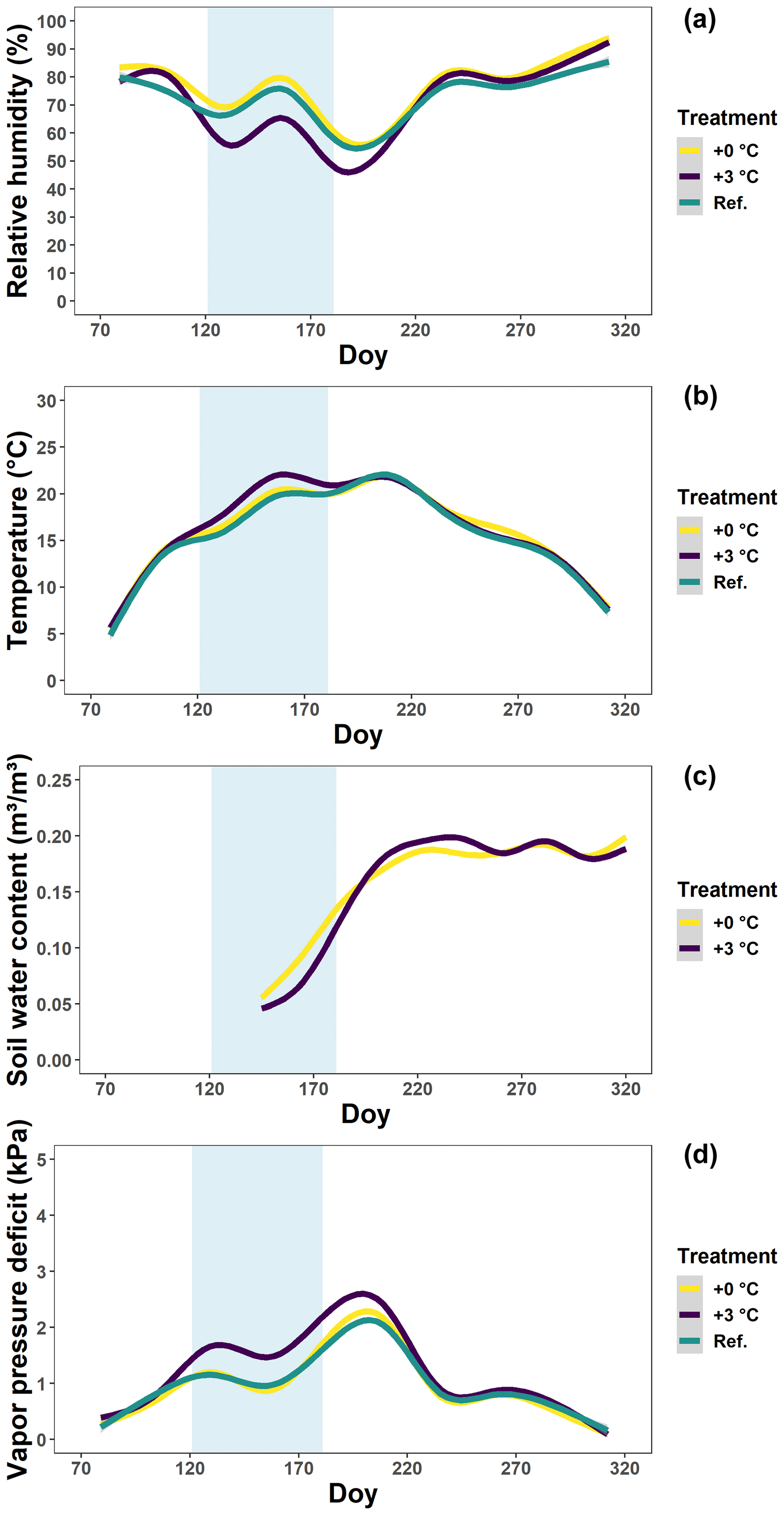
Figure 1 The relative humidity (a), temperature (b), soil water content (c) and vapor pressure deficit (d) in the glasshouses and outside plots at the Drie Eiken Campus in Wilrijk. Solid lines represent regressions of half-hourly measurements of the relative humidity (%), temperature (^∘C) and soil water content (m³/m³). Regressions were performed using generalized additive models implemented by the geom_smooth argument in the R ggplot2 package. The vapor pressure deficit (kPa) was calculated using the formulas of Buck (1981) using data of the relative humidity and air temperature between 07:00 and 19:00 CET. Green, yellow and purple lines represent the conditions in the reference plots (Ref.), glasshouses that follow the outside ambient air temperature (+0 ^∘C) and glasshouses that are 3 ^∘C warmer than the outside ambient air temperature (+3 ^∘C), respectively. The light blue band represents the treatment-period.

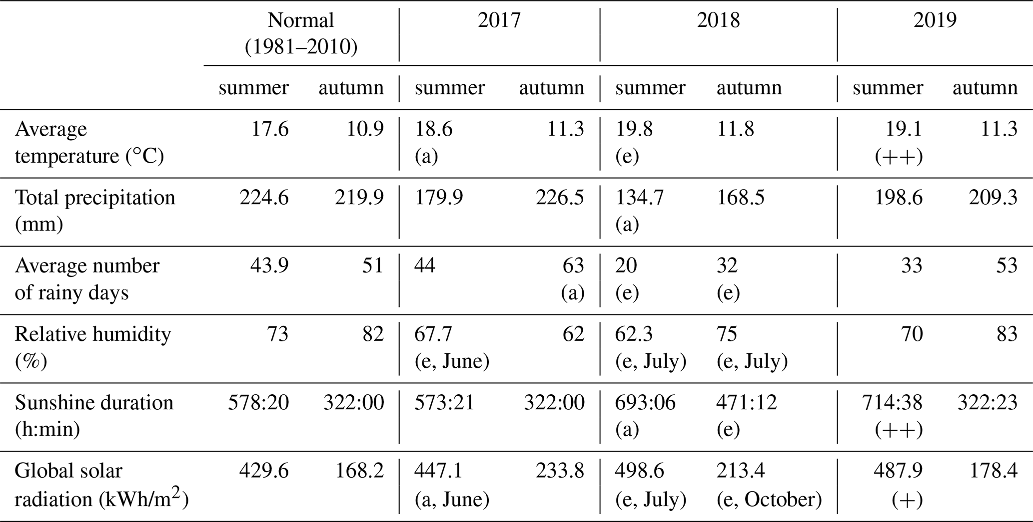
Table 1 Overview of the meteorological conditions during the summer and autumn of 2017, 2018 and 2019. All data are measured by the meteorological station of the Royal Meteorological Institute (KMI) in Ukkel, Belgium (KMI, 2018a, b, 2017b, a, 2019a, b). The degree of abnormality of the values is represented by two labels: a for abnormal values (with a recurrence time of 6 years) or e for exceptional values (with a recurrence time of 30 years). In the case only 1 month had abnormal values, this label is followed by the name of that particular month. Since 2019, the KMI has used a new system to show the degree of abnormality: values that are among the five highest values since 1981 are marked by (+), while values within the three highest values are marked by ($++)$.

From planting until April, the saplings were all irrigated two to three times a week until the pots overflowed. The reference plots outside were maintained with abundant irrigation during the whole growing season. On the other hand, at the start of the treatment, in early May, we shielded all the glasshouses using polyethylene film (200 µm thick) and irrigated the saplings only once a week with circa 2.5 L of water. In addition, we enhanced the drought in six glasshouses by raising the air temperature by 3 ^∘C compared to the ambient air temperature (+3 ^∘C). The air temperature in the other six glasshouses followed the ambient air temperature (+0 ^∘C). There were no significant differences in the temperature, relative humidity and vapor pressure deficit among the glasshouses with the reference and +0 ^∘C treatment (Fig. 1). Although no data on the soil water content were available for the reference plots (due to sensor malfunctioning), we did not expect major drought stress due to their abundant irrigation and lack of stress signals. Based on this information, the +0 ^∘C treatment can be considered a “less irrigation or drought” treatment. On the other hand, during the treatment, the daily soil water content and the daily relative humidity in the glasshouses with the +3 ^∘C treatment were significantly lower (P<0.001; tested using generalized additive mixed models) in comparison to the glasshouses with the +0 ^∘C treatment. After statistical testing following Rose et al. (2012), the difference between the +0 and +3 ^∘C treatments was found to be around 0.025 m³/m³ for the soil water content and 20 % for the relative humidity (Fig. 1; see “Data availability”). The +3 ^∘C treatment can therefore be considered a combined “less irrigation or drought, warming, and increased atmospheric aridity” treatment. In fact, this treatment should simulate natural drought conditions, which are often associated with heat stress and increased atmospheric aridity. The plan was to continue the treatment till the end of June, but, due to the significant mortality rate, we were already obliged to alleviate the drought from the 20 June by increasing the irrigation to the level of the reference plots. From July, the glasshouses were opened again and the saplings were irrigated four to five times a week until the end of the season.

A drawback of the experiment is that the saplings in the reference plots received more incoming light (i.e., ±20 %) than the saplings in the glasshouses (Van den Berge et al., 2011). However, as beech is a shade-tolerant species, reduced light is unlikely to have limited tree growth. In addition, preliminary tests suggested that the ratio of light on different wavelengths (e.g., R/FR) during civil twilight (i.e., what is required for phytochrome to detect the photoperiod) does not change seasonally significantly in our study area (Chelle et al., 2007).

2.1.2 Field observations in deciduous forests

From 2017 to 2019, we monitored dominant mature trees in two forests near Antwerp: the Klein Schietveld in Kapellen (KS; 51^∘21^′ N, 4^∘37^′ E) and the Park of Brasschaat (PB; 51^∘12^′ N, 4^∘26^′ E). In the KS, we monitored eight beech trees and eight birch (Betula pendula) trees. In the PB, we monitored eight beech trees and eight oak (Quercus robur) trees (thus 32 trees in total). The two forests and their meteorological conditions are described in detail by Mariën et al. (2019), which also show a lack of site effects on the autumn chlorophyll dynamics for the tree species studied here. To have a larger statistical sample, the data of the two beech stands (also of similar age and stem diameter) were aggregated.

For summer and autumn, we report here the average values for the temperature, precipitation, number of rainy days, relative humidity, sunshine duration and global solar radiation for the meteorological station of the Royal Meteorological Institute (KMI) in Ukkel, Belgium (Table 1). For these data, long-term averaged data were available. The temperature, relative humidity, vapor pressure deficit (see Eq. 1), precipitation and volumetric soil water content from 2017 to 2019 are presented in more detail using daily values that were measured at Brasschaat and, whenever necessary, gap-filled with data from the meteorological station in Woensdrecht, the Netherlands (Fig. 2a, b, d). The meteorological data from Brasschaat were provided by the Flemish Institute for Nature and Forest (INBO) and the Integrated Carbon Observation System (ICOS), while the data from Woensdrecht were provided by the Royal Netherlands Meteorological Institute (KNMI).

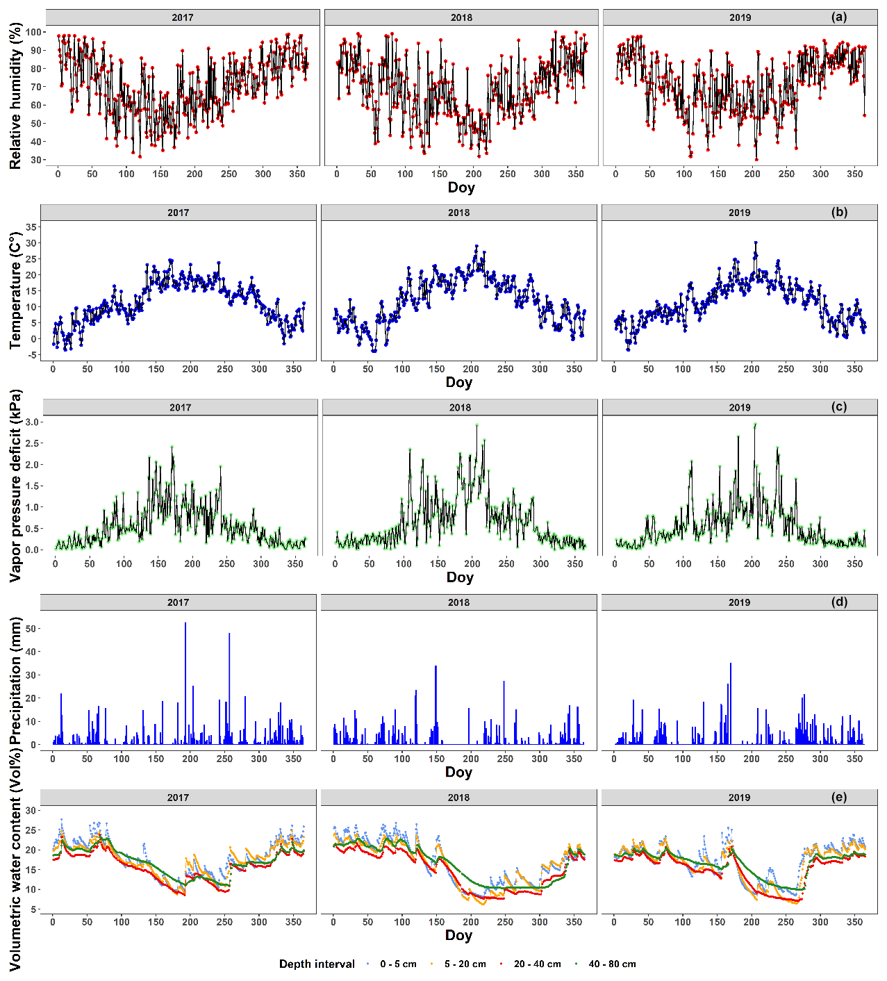
Figure 2 The meteorological conditions near the Klein Schietveld and Park of Brasschaat. The line plots represent the daily average relative humidity (%; red), temperature (^∘C; blue) and vapor pressure deficit (kPa; green). The bar plots represent the daily precipitation (mm; light blue). The volumetric soil water content (Vol %) at depth intervals of 0–5, 5–20, 20–40 and 40–80 cm is presented as line plots in cornflower blue, orange, red and green, respectively. The relative humidity, temperature, vapor pressure deficit and precipitation data were measured every half hour and provided by the Flemish Institute for Nature and Forest (INBO), the Integrated Carbon Observation System (ICOS), and the Royal Netherlands Meteorological Institute (KNMI). The vapor pressure deficit (kPa) was calculated using the formulas of Buck (1981) using data of the relative humidity and air temperature between 07:00 and 19:00 CET. The volumetric soil water content data were first measured every 6 h, but after 3 July 2018 measurements were made every hour. The volumetric soil water content data were provided courtesy of INBO.

The distance from Ukkel and Woensdrecht to our sites is 60 and 20 km, respectively. However, both locations show no major climatological differences with the KS and PB and are representative of the inter-annual variability experienced by the forests. The station of Ukkel is located within a green area in the suburb of Brussels (thus, classifiable as “urban park”). The microclimate is expected to be different than at our study sites. However, data from Ukkel were used to describe the intra-annual variability and long-term trends in the meteorological variables, which are less affected by the microclimate. The meteorological station of Brasschaat is very close to our sampling sites in the Park of Brasschaat and in the Klein Schietveld (±3 and ±4 km, respectively). The meteorological station in Brasschaat is a 40 m high scaffolding tower, at which measurements are taken at various heights, and stands in a patch of mixed forest covered mainly by Scots pines and deciduous tree species, such as oak and birch (see Carrara et al., 2003, for more information). Data of the temperature, precipitation and humidity were taken at the top of the tower. Concurrently, the volumetric soil water content was measured near the scaffolding tower using 12 water reflectometers (CS616 Water Content Reflectometer, Campbell Scientific, UT, USA) connected to a central data logger (CR1000 data logger, Campbell Scientific, UT, USA). The water reflectometers were equally divided over three sampling pits at an 8 m distance from the central data logger. In 2010 and in each pit, the water reflectometers were installed in pedogenetic horizons at four depth intervals (i.e., 0–5, 5–20, 20–40 and 40–80 cm). The volumetric soil water content data were first measured every 6 h, but after 3 July 2018 measurements were made every hour. The volumetric soil water content was calibrated following De Vos (2016) and averaged per day and depth interval. The station of Woensdrecht is located in an open field at a local airport surrounded by heathland and an urban area. It is located near the Markiezaatsmeer, an enclosed swamp ecosystem, within the river mouth of the Scheldt. The measurements in both Ukkel and Woensdrecht are taken at a height of 1.5 m. However, these data were only used as gap filling in the case of short-term gaps in the long-term Brasschaat series.

2.1.3 The rainfall deficit – an indicator of drought stress for 2017–2019

To indicate the magnitude of the droughts, we computed the rainfall deficit from 2017 to 2019 using data on the relative humidity, solar radiation, wind speed, temperature and precipitation from the meteorological station in Ukkel. Here, the meteorological records go back the longest in Belgium. The rainfall deficit is computed on a daily basis by accumulating the daily potential evapotranspiration minus the daily amount of precipitation. This was done in two ways: (I) per hydrological year, starting from a zero deficit at the start of the hydrological year (1 April) and (II) continuous computation, i.e., no restart from 0 at the start of each hydrological year. The latter method has the benefit that the long-term effect of accumulated droughts from successive years is accounted for.

The potential evapotranspiration was computed by means of the method of Bultot et al. (1983), which is similar to the method of Penman (1948) but has parameters that are calibrated specifically for the local Belgian conditions. Unlike for the rainfall deficit starting from a zero deficit, we accounted in the calculation of the continuously computed rainfall deficit for the hydrological fraction in wet periods that does not contribute to building up groundwater reserves. At the station of Ukkel, daily precipitation and potential evapotranspiration data are available covering more than 100 years. The precipitation data have been collected since 1898 at the same location and have been measured using the same instrument. For this study, the data for the 100-year period 1901–2000 were considered the reference data for the computation of long-term statistics on the rainfall deficit.

2.2 Measuring autumn leaf senescence – the chlorophyll content index and the loss of canopy greenness

In the manipulative experiment from late July until late November, we measured the chlorophyll content index (CCI; a proxy for the chlorophyll concentration) of each tree sapling weekly by randomly selecting one leaf from the outer, middle and inner layer of the upper part of the crown. The CCI was measured using a chlorophyll content meter, which measures the optical absorbance in the 653 and 931 nm wavebands (CCM-200 plus, Opti-Sciences Inc., Hudson, NH, USA). Concurrently, we visually estimated the loss of canopy greenness (LOCG; scaled between 0 and 1) of each sapling following the method of Vitasse et al. (2011), which accounts for both the percentage of leaves that have changed color and the percentage of leaves that have fallen.

For half of the monitored mature trees in the two forests and from the end of July to the end of November, tree climbers collected leaves on eight occasions per year separated by 2 to 3 weeks. During each measurement day, they collected five sun leaves and five shade leaves from each tree. Afterwards, the CCI was immediately measured on the harvested leaves using the same chlorophyll content meter as described above. From early September to late November, the loss of canopy greenness was estimated in a similar fashion to the manipulative experiment for the 32 mature trees (Vitasse et al., 2011).

Following the method of Mariën et al. (2019), we validated the CCI values by also measuring the chlorophyll concentrations (Fig. A1). In 2017 and 2018, on one occasion per month and using a 10 mm diameter cylinder, we collected samples of leaf tissue from the leaves of the mature trees for which we also measured the CCI. After storage at −80 ^∘C, the samples were grounded using glass beads and a centrifuge. The result was dissolved in ethanol, and the absorption of the solution was measured using a spectrophotometer (SmartSpec Plus spectrophotometer, Bio-Rad) at different wavelengths for chlorophyll a (662 nm) and chlorophyll b (644 nm). The chlorophyll concentrations could then be derived from the absorption values using the formulas described in Holm (1954) and Vonwettstein (1957).

2.3 Tree mortality in the manipulative experiment

In this study, we only considered those trees that defoliated due to autumn leaf senescence. Other tree saplings died or defoliated completely due to accelerated leaf senescence during or just after the treatment period. Since chlorophyll degradation is a common feature of both senescence processes and nutrient remobilization was only measured indirectly by the CCI, we did not consider (I) tree saplings that showed an early or abrupt defoliation (without gradual coloration) before the 18 August (n=20) and (II) tree saplings with constant CCI values lower than 3, the limit at which the values of the CCI meter can be interpreted, for the whole period from August to November (n=18). Like in other studies, some defoliated tree saplings produced a few new leaves as a last attempt to prevent death (Vander Mijnsbrugge et al., 2016; Turcsan et al., 2016). However, there were not enough of such leaves for meaningful analyses.

2.4 Statistical analyses

All statistical analyses were performed using R v.3.6.1 (R Core Team, 2020). The model assumptions were tested following Zuur et al. (2010). All graphical output is built using the R packages ggplot2, ggpubr, viridis and cowplot, while data manipulation has been performed using the R package dplyr (Wickham, 2009; Wilke, 2019; Garnier, 2018; Kassambara, 2019; Wickham et al., 2018).

2.4.1 Assessing the patterns of CCI and loss of canopy greenness using generalized additive mixed models

The patterns of the CCI and loss of canopy greenness data from both our tree saplings and mature trees were assessed using generalized additive mixed models (GAMMs) built using the R packages mgcv and gratia (Wood, 2011; Simpson, 2020; Hastie and Tibshirani, 1986; Pedersen et al., 2019). We used GAMMs because they allow more flexibility than other models (e.g., generalized linear models) to model the distribution parameter μ (i.e., the mean of the observed random variable) and the continuous explanatory variables (Rigby and Stasinopoulos, 2005).

To model the CCI of both our tree saplings and mature trees as a function of their covariates, Gaussian GAMMs with the identity link function were used (Table 2). To model the loss of canopy greenness of both our tree saplings and mature trees as a function of their covariates and because the loss of canopy greenness is scaled between 0 and 1, binomial GAMMs with the logistic link function were used (Table 2). The GAMMs were chosen with the lowest AIC (Akaike information criterion) value and all factor–smooth interaction terms were smoothed using P-splines to address the large gap in data (i.e., from November to June) between the yearly sampling periods.

Table 2 Adjusted R², effective degrees of freedom (edf's) and F-test values of the GAMM smooth terms (day of the year). All smooth terms were significant, with P values <0.001. 𝔼(y_i) values are the expected values of the response variable y_i; f(x_i) is the smooth function of the covariate x_i; β_i is the intercept of the covariate x_i; ζ is the random effect, and ε_i values are the errors. All smooth functions were fitted using P-splines. The chlorophyll content index, day of the year and tree individual are abbreviated by CCI, DOY and ID, respectively.

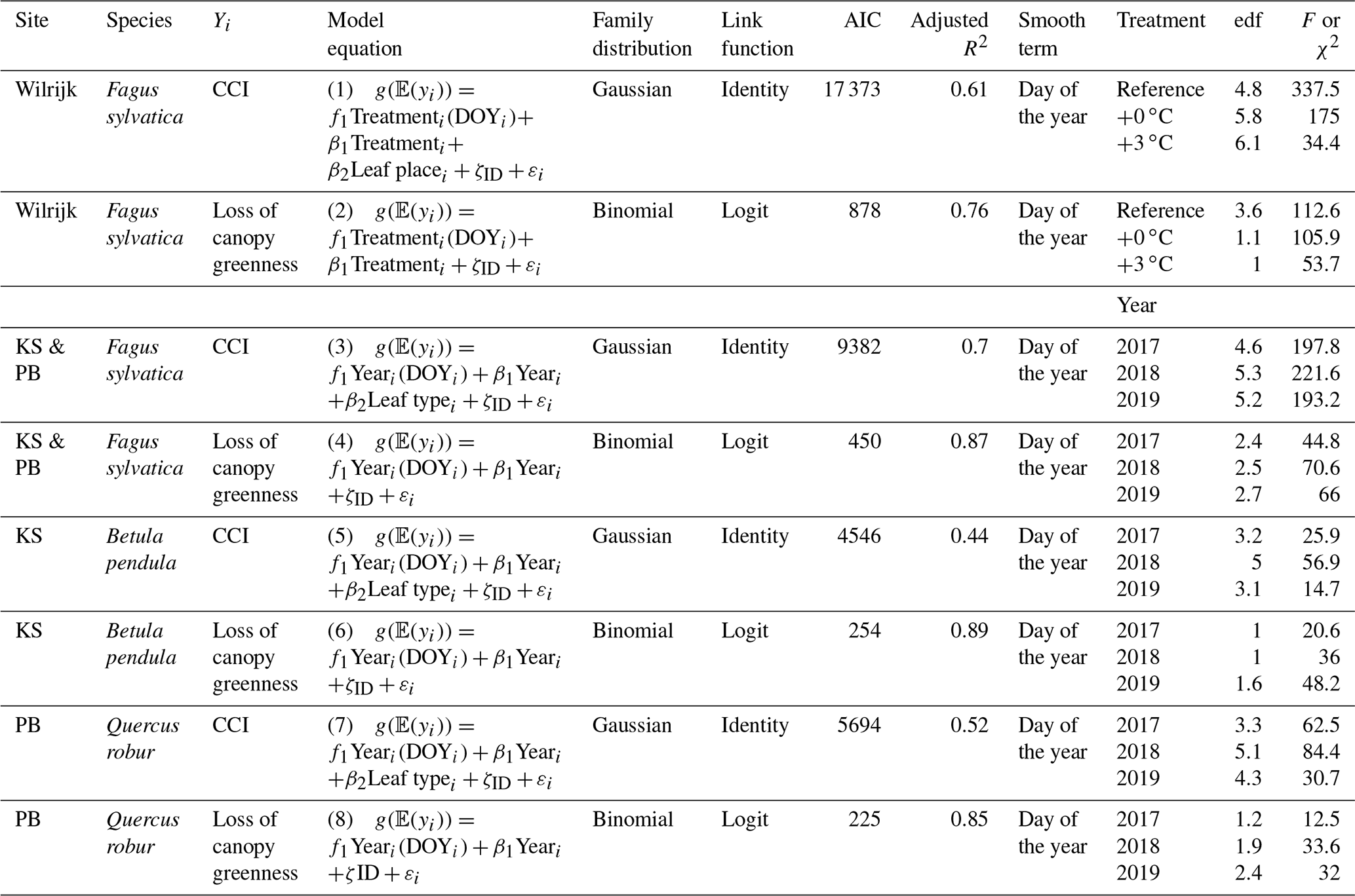
For the CCI of the beech saplings, the fixed covariates were the treatment (categorical with three levels), leaf place (categorical with three levels) and day of the year (continuous; model 1). The interaction term was modeled as a factor–smooth interaction between the covariates day of the year and treatment. The dependency among observations of the same individual tree was incorporated by using individual tree as the random intercept (in the following, the abbreviation cst. denotes “constant”).

$$\begin{array}{}\text{(Model 1)}& \begin{array}{rl}& Y_{ij}\sim \mathrm{Gaussian}({\mathit{\mu }}_{ij},\mathrm{cst}.),\\ & g\left(\mathbb{E}\right(Y_{ij}\left)\right)=g\left({\mathit{\mu }}_{ij}\right),\\ & g\left({\mathit{\mu }}_{ij}\right)={\mathrm{Treatment}}_{ij}+\mathrm{Leaf}{\mathrm{place}}_{ij}\\ & +f(\mathrm{Day}\mathrm{of}\mathrm{the}{\mathrm{year}}_{ij},{\mathrm{Treatment}}_{ij})\\ & +\mathrm{Individual}{\mathrm{tree}}_i,\end{array}\end{array}$$

where g is the identity link function; μ_ij is the conditional mean; Y_ij is the jth observation of the response variable (i.e., the CCI) in individual tree i, with i=1, …, 128; and Individual tree_i is the random intercept (Zuur et al., 2007, 2016).

For the loss of canopy greenness of the beech saplings, the fixed covariates were the treatment (categorical with three levels) and day of the year (continuous; model 2). The interaction term and the dependency among observations of the same individual tree were treated as in model 1.

$$\begin{array}{}\text{(Model 2)}& \begin{array}{rl}& Y_{ij}\sim B(n_{ij},{\mathit{\pi }}_{ij}),\\ & g\left(\mathbb{E}\right(Y_{ij}\left)\right)=g\left({\mathit{\mu }}_{ij}\right),\\ & g\left({\mathit{\mu }}_{ij}\right){=}_{}{\mathrm{Treatment}}_{ij}+f(\mathrm{Day}\mathrm{of}\mathrm{the}{\mathrm{year}}_{ij},\\ & {\mathrm{Treatment}}_{ij})+\mathrm{Individual}{\mathrm{tree}}_i,\end{array}\end{array}$$

where n_ij is the number of observations; π_ij is the probability of “success”; g is the logit link function; μ_ij is the conditional mean; Y_ij is the jth observation of the response variable (i.e., the loss of canopy greenness) in individual tree i, with i=1, …, 128; and Individual tree_i is the random intercept.

For the CCI of the mature beech, birch and oak trees, the fixed covariates were the year (categorical with three levels), leaf type (categorical with two levels) and day of the year (continuous; model 3). The interaction term was modeled as a factor–smooth interaction between the covariates day of the year and year. The dependency among observations of the same individual tree was incorporated using individual tree as the random intercept.

$$\begin{array}{}\text{(Model 3)}& \begin{array}{rl}& Y_{ij}\sim \mathrm{Gaussian}({\mathit{\mu }}_{ij},\mathrm{cst}.),\\ & g\left(\mathbb{E}\right(Y_{ij}\left)\right)=g\left({\mathit{\mu }}_{ij}\right),\\ & g\left({\mathit{\mu }}_{ij}\right){=}_{}{\mathrm{Year}}_{ij}+\mathrm{Leaf}{\mathrm{type}}_{ij}\\ & +f(\mathrm{Day}\mathrm{of}\mathrm{the}{\mathrm{year}}_{ij},{\mathrm{Year}}_{ij})\\ & +\mathrm{Individual}{\mathrm{tree}}_i,\end{array}\end{array}$$

where g is the identity link function; μ_ij is the conditional mean; Y_ij is the jth observation of the response variable (i.e., the CCI) in individual tree i, with i=1, …, 8 for beech, i=1, …, 4 for birch and i=1, …, 4 for oak; and Individual tree_i is the random intercept.

For the loss of canopy greenness of the mature beech, birch and oak trees, the fixed covariates were the year (categorical with three levels) and day of the year (continuous; model 4). The interaction term and the dependency among observations of the same individual tree were treated as in model 3.

$$\begin{array}{}\text{(Model 4)}& \begin{array}{rl}& Y_{ij}\sim B(n_{ij},{\mathit{\pi }}_{ij}),\\ & g\left(\mathbb{E}\right(Y_{ij}\left)\right)=g\left({\mathit{\mu }}_{ij}\right),\\ & g\left({\mathit{\mu }}_{ij}\right){=}_{}{\mathrm{Year}}_{ij}+\mathit{\text{f}}(\mathrm{Day}\mathrm{of}\mathrm{the}{\mathrm{year}}_{ij},{\mathrm{Year}}_{ij})\\ & +\mathrm{Individual}{\mathrm{tree}}_i,\end{array}\end{array}$$

where n_ij is the number of observations; π_ij is the probability of success; g is the logit link function; μ_ij is the conditional mean; Y_ij is the jth observation of the response variable (i.e., the loss of canopy greenness) in individual tree i, with i= 1, …, 16 for beech, i=1, …, 8 for birch and i=1, …, 8 for oak; and Individual tree_i is the random intercept.

2.4.2 Using breakpoints to indicate the onset of autumn leaf senescence and the onset of the loss of canopy greenness

In principle, the onset of autumn leaf senescence could be derived from the CCI or loss of canopy greenness. However, Mariën et al. (2019) recently showed that the latter method cannot be used under severe drought stress. Therefore, two phenological variables were considered to describe the autumn canopy dynamics: the onset of autumn leaf senescence derived from the CCI (the onset of autumn leaf senescence) and the onset of the loss of canopy greenness. For each tree, we defined the onset of autumn leaf senescence and the onset of loss of canopy greenness as the date by which the variable of interest started to decline substantially in early autumn. These dates were calculated using piecewise linear regressions and are represented by the breakpoints resulting from these analyses (Menzel et al., 2015; Mariën et al., 2019; Xie and Wilson, 2020). The piecewise linear regressions were performed using the R package segmented (Vito and Muggeo, 2008). The uncertainty reported represents the inter-tree variability. Trees that did not show a clear breakpoint (13 in the manipulative experiment) were not considered in the analysis. These trees did not show a different pattern of CCI or loss of canopy greenness than the other trees (Fig. A2).

2.4.3 Comparing the onset of autumn leaf senescence among tree saplings exposed to different treatments

We tested whether the beech saplings exposed to the three treatments in 2018 differed in their onset of autumn leaf senescence using a linear model with the onset of autumn leaf senescence as the response variable and treatment (categorical with three levels) as the fixed covariate. The residuals of the model were approximately normally distributed and a Breusch–Pagan test, the ncvTest and bptest functions in the car and lmtest R packages showed no evidence of heteroscedasticity (P>0.05) (Fox and Weisberg, 2019; Zeileis and Hothorn, 2002). A one-way ANOVA was used to detect significant differences in the onset of autumn leaf senescence among the treatments.

2.4.4 Comparing the onset of autumn leaf senescence and the onset of loss of canopy greenness in mature trees among species and years

To model the onset of autumn leaf senescence and the onset of the loss of canopy greenness as a function of their covariates, Gaussian linear mixed models were used. These models were built with the R package lme4 (Bates et al., 2015).

The effect of the year on the onset of autumn leaf senescence and the onset of the loss of canopy greenness was assessed using two linear mixed-effect models with the onset of autumn leaf senescence and the onset of the loss of canopy greenness from the mature beech, birch and oak trees as the response variable. The fixed covariate in these two models was the year (categorical with three levels; model 5). To incorporate the dependency among observations of the same species, we used species as the random intercept.

$$\begin{array}{}\text{(Model 5)}& \begin{array}{rl}& Y_{ij}\sim \mathrm{Gaussian}({\mathit{\mu }}_{ij},\mathrm{cst}.),\\ & g\left(\mathbb{E}\right(Y_{ij}\left)\right)=g\left({\mathit{\mu }}_{ij}\right),\\ & {\mathit{\mu }}_{ij}={\mathrm{Year}}_{ij}+{\mathrm{Species}}_i,\end{array}\end{array}$$

where g is the identity link function; μ_ij is the conditional mean; Y_ij is the jth observation of the response variable in species i, with i=1, …, 3; and Species_i is the random intercept.

The effect of the species on the onset of autumn leaf senescence and the onset of the loss of canopy greenness was assessed using two linear mixed-effect models with the onset of autumn leaf senescence and the onset of the loss of canopy greenness from the mature beech, birch and oak trees as the response variable. The fixed covariate in these two models was the species (categorical with three levels; model 6). To incorporate the dependency among observations of the same year, we used year as the random intercept.

$$\begin{array}{}\text{(Model 6)}& \begin{array}{rl}& Y_{ij}\sim \mathrm{Gaussian}({\mathit{\mu }}_{ij},\mathrm{cst}.),\\ & g\left(\mathbb{E}\right(Y_{ij}\left)\right)=g\left({\mathit{\mu }}_{ij}\right),\\ & {\mathit{\mu }}_{ij}={\mathrm{Species}}_{ij}+{\mathrm{Year}}_i,\end{array}\end{array}$$

where g is the identity link function; μ_ij is the conditional mean; Y_ij is the jth observation of the response variable in year i, with i= 1, …, 3; and Year_i is the random intercept.

The residuals of the models were approximately normally distributed and showed no heteroscedasticity (tested using diagnostic plots). Therefore, we used Pearson's χ² test, drop1 in the lme4 R package, to detect significant differences in the onset of autumn leaf senescence and the onset of the loss of canopy greenness among the predictor variables. A multiple comparison test, the glht test with Tukey's method in the multcomp R package, was used to test for significant differences among the means of the levels in the predictor variables (Hothorn et al., 2008).

3 Results

3.1 Magnitude of the drought stress in 2017, 2018 and 2019

The weather in 2018 and 2019 was exceptional, as can be seen in the overview of the meteorological conditions from 2017 to 2019 against the long-term reference values in Table 1 and Fig. 2. In 2017, the weather during spring was dry and warm but the weather during summer and autumn was relatively normal (KMI, 2017b, a, c). In contrast, the warm and dry summer of 2018 was marked by abnormal (with an average return time of 6 years) to exceptional (with an average return time of 30 years or more) values (KMI, 2018b). Furthermore, the autumn of 2018 was abnormally dry and all precipitation fell on relatively few days (32) (KMI, 2018a). In the summer of 2019, both the average air temperature and the total amount of sunshine were among the three highest values recorded since 1981. In fact, the absolute maximum air temperature record for Belgium was broken in 2019 (KMI, 2019b). On the other hand, the autumn of 2019 was considered normal (KMI, 2019a).

The rainfall deficit for each day in the hydrological year (from the 1 April until the 31 March) and different return times are shown in Fig. 3a and b. This demonstrates that in the late spring of 2017, the summer of 2018 and the summer of 2019, the rainfall deficit reached a return time of between 20 and 50 years, 50 years, and 20 years, respectively. The hydrological summers of 2017, 2018 and 2019 had therefore moderate to extremely dry conditions, which led to accumulated rainfall deficit conditions over time (see Fig. 3a). Especially the hydrological year starting in 2018 ended with a strong rainfall deficit of about 150 mm, which was not reduced during 2019. The effects of this strong rainfall deficit are also apparent in the lower volumetric soil water content values (ca. 5 % less) measured at the beginning of 2019, compared to the same measurements in 2017 and 2018.

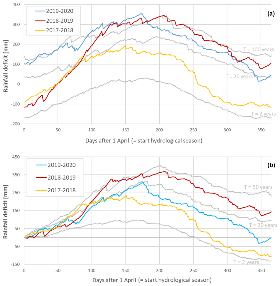
Figure 3 The rainfall deficit for the meteorological station of the Royal Meteorological Institute (KMI) in Ukkel, Belgium. The solid colored lines represent the rainfall deficit for the hydrological years in the period 2017–2020, while the solid grey lines represent the long-term reference statistics (computed for the 100-year period 1901–2000) with T as the return period, which represents the mean time between two successive exceedances of a given deficit value and is computed in an empirical way (Willems, 2000, 2013). Panel (a) uses a continuous computation, while panel (b) starts from a zero deficit on the first of April (the start of the hydrological year). The colors represent the rainfall deficit in 2017 (light blue), 2018 (red) and 2019 (yellow).

3.2 The effect of drought, heat stress and increased atmospheric aridity on the onset of autumn leaf senescence in tree saplings in the manipulative experiment

For all treatments, the CCI values of the beech saplings showed an overall moderate decrease until the beginning of October. Afterwards, this decrease accelerated (Fig. 4a, c; Table 2). In the +0 ^∘C and especially the +3 ^∘C treatment, an abnormal CCI decline was observed in early August with only a partial recovery later on. As a result, from the beginning of August until mid-September, the CCI values of the beech saplings in the reference plots were significantly higher than the CCI values of the beech saplings in the glasshouses. From the end of September, the CCI decreased in all treatments, showing similar CCI measurements across treatments. However, the modeled CCI of the +3 ^∘C treatment declined more slowly than the modeled CCI of the other two treatments. No significant difference was detected in the timing of the onset of autumn leaf senescence among the beech saplings exposed to the three different treatments, as the mean onset of autumn leaf senescence was between 21 (DOY $=\mathrm{260}\pm \mathrm{5}$) and 25 (DOY $=\mathrm{264}\pm \mathrm{4}$) September (P=0.7; Fig. A3).

Figure 4 The generalized additive mixed model fits for the chlorophyll content index (CCI; a) and loss of canopy greenness (b) of the Fagus sylvatica saplings at the Drie Eiken Campus in Wilrijk. The solid colored lines represent smooth terms, while the colored shaded bands around the smooth terms approximate the 95 % simultaneous confidence intervals (a) and 95 % pointwise confidence intervals (b). The dots and error bars represent the mean CCI (c) and mean canopy greenness (d) with standard errors. The colors represent the CCI or the loss of canopy greenness of the beech saplings in the reference plots (green; Ref.), the glasshouses that followed the outside ambient air temperature (yellow; +0 ^∘C) and the glasshouses that were 3 ^∘C warmer than the outside ambient air temperature (purple; +3 ^∘C).

The canopy greenness for the beech saplings showed a stable decline from early August until the end of autumn (Fig. 4b, d; Table 2). Nevertheless, during September, the canopy greenness of the beech saplings in the reference plots was significantly higher than the canopy greenness of the beech saplings in the glasshouses with the +3 ^∘C treatment.

The tree saplings in the glasshouses of both treatments were exposed to a high mortality with 14 % and 26 % of the tree saplings in the glasshouses with the +0 and +3 ^∘C treatment, respectively, considered “dead” according to our criteria (see Sect. 2.3.). In the reference plots, no beech saplings died.

3.3 Inter-annual and inter-species variability in the timing of the onset of autumn leaf senescence and the onset of the loss of canopy greenness in mature trees

The pattern in the CCI values for the mature beech, birch and oak trees seems consistent throughout the years with stable values in summer and a rapid decline around late October (panels a–c in Figs. 5–7; Table 2). We also observed no significant difference in the onset of autumn leaf senescence among the years (P=0.09) and species (P=1). The mean onset of autumn leaf senescence among the years was from 8 (DOY $=\mathrm{281}\pm \mathrm{6}$) to 19 (DOY $=\mathrm{292}\pm \mathrm{6}$) October (Fig. A4a), while the mean onset of autumn leaf senescence among the species was around 13 October (DOY $=\mathrm{286}\pm \mathrm{6}$; Fig. A4b). The CCI correlated linearly with the chlorophyll concentrations, but the data showed more variation in 2018 than 2017 (see Fig. A1).

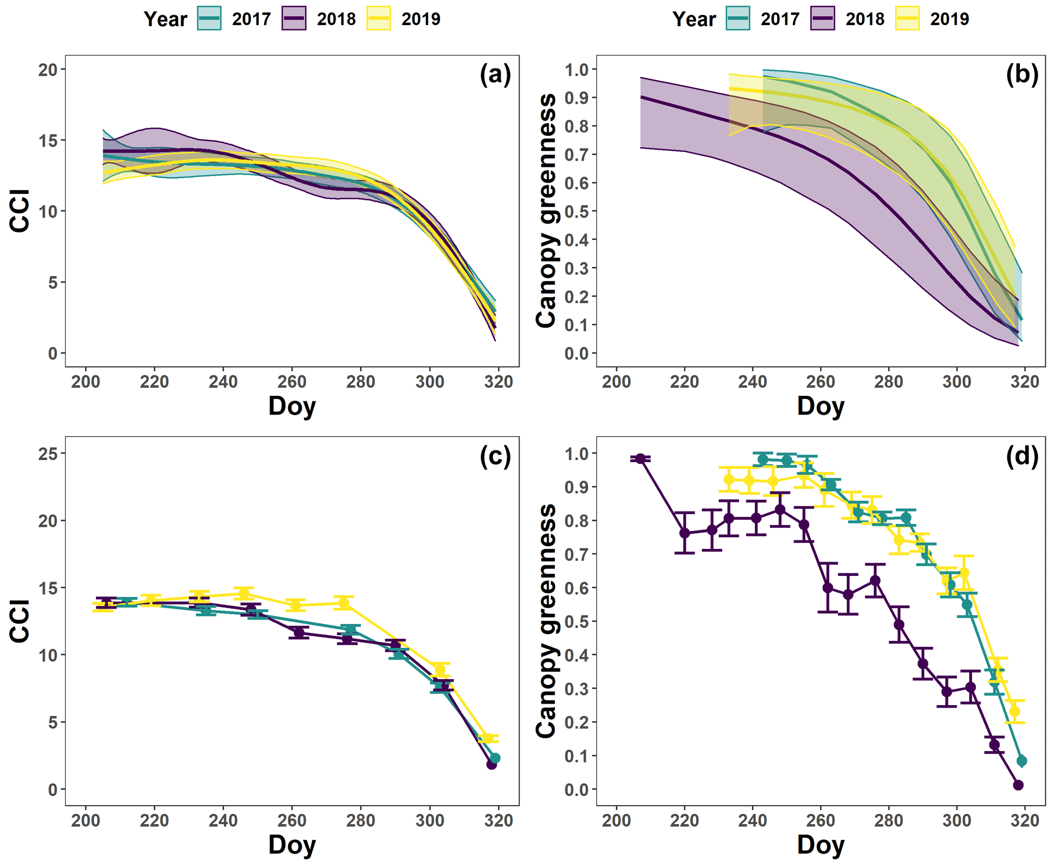
Figure 5 The generalized additive mixed model fits for the chlorophyll content index (CCI; n=8; a) and loss of canopy greenness (n=16; b) of the mature Fagus sylvatica trees at the Klein Schietveld and Park of Brasschaat. The solid colored lines represent smooth terms, while the colored shaded bands around the smooth terms represent approximate 95 % simultaneous confidence intervals (a) and 95 % pointwise confidence intervals (b). The dots and error bars represent the mean CCI (c) and mean canopy greenness (d) with standard errors. The colors represent the CCI or the loss of canopy greenness of the mature beech trees in 2017 (green), 2018 (purple) and 2019 (yellow).

Figure 6 The generalized additive mixed model fits for the chlorophyll content index (CCI; n=4; a) and loss of canopy greenness (n=8; b) of the mature Betula pendula trees at the Klein Schietveld. The solid colored lines represent smooth terms, while the colored shaded bands around the smooth terms represent approximate 95 % simultaneous confidence intervals (a) and 95  % pointwise confidence intervals (b). The dots and error bars represent the mean CCI (c) and mean canopy greenness (d) with standard errors. The colors represent the CCI or the loss of canopy greenness of the mature birch trees in 2017 (green), 2018 (purple) and 2019 (yellow).

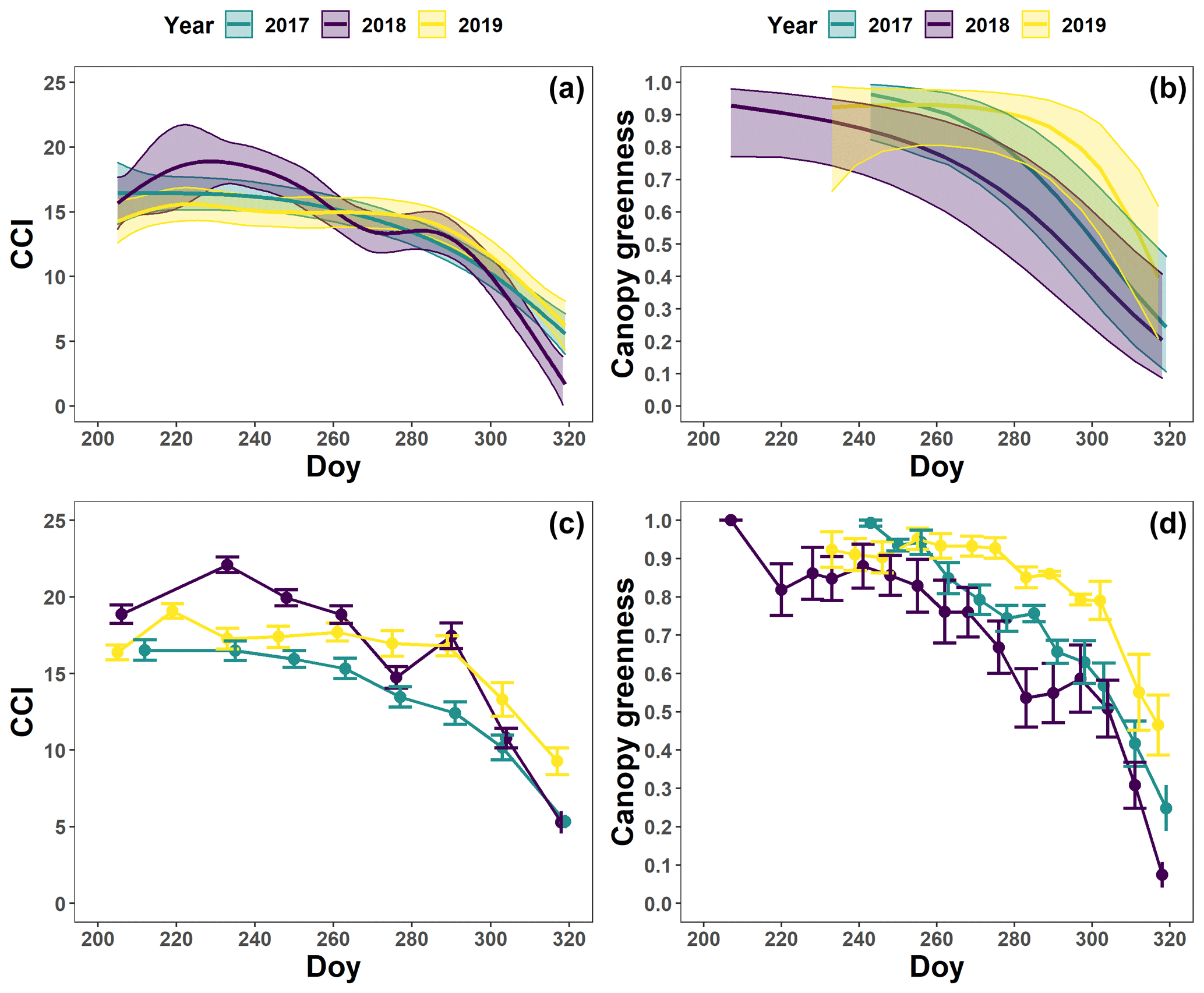
Figure 7 The generalized additive mixed model fits for the chlorophyll content index (CCI; n=4; a) and loss of canopy greenness (n=8; b) of the mature Quercus robur trees at the Park of Brasschaat. The solid colored lines represent smooth terms, while the colored shaded bands around the smooth terms represent approximate 95 % simultaneous confidence intervals (a) and 95 % pointwise confidence intervals (b). The dots and error bars represent the mean CCI (c) and mean canopy greenness (d) with standard errors. The colors represent the CCI or the loss of canopy greenness of the mature oak trees in 2017 (green), 2018 (purple) and 2019 (yellow).

The pattern in the canopy greenness for the mature beech, birch and oak trees seemed less consistent throughout the years (panels b and d in Figs. 5–7; Table 2). The loss of canopy greenness showed a very similar pattern between 2017 and 2019 for birch and beech, with the start of the decline in canopy greenness values around late September for birch and late October for beech. Like beech and birch, oak showed a standard pattern in 2019 with the start of the seasonal decline in late October. However, in 2017, oak showed an earlier loss of canopy greenness with the start of the seasonal decline in mid-September. In all cases, a rapid decline in the canopy greenness was observed in late autumn. In 2018, all species showed an earlier and steeper decline in their canopy greenness values. This effect was also reflected by a significant difference in the onset of the loss of canopy greenness among the years ($P=\mathrm{5}\times {\mathrm{10}}^{-\mathrm{11}}$). Across species, the onset of the loss of canopy greenness did not differ significantly (P=0.9) between 2017 (DOY $=\mathrm{292}\pm \mathrm{9}$) and 2019 (DOY $=\mathrm{290}\pm \mathrm{4}$), while it occurred 26 and 25 d earlier in 2018 (DOY $=\mathrm{266}\pm \mathrm{4}$) compared to 2017 ($P=\mathrm{1}\times {\mathrm{10}}^{-\mathrm{5}}$) and 2019 ($P=\mathrm{1}\times {\mathrm{10}}^{-\mathrm{5}}$), respectively (Fig. A5a). However, all tree species differed significantly in their onset of the loss of canopy greenness across years ($P=\mathrm{6}\times {\mathrm{10}}^{-\mathrm{9}}$). Compared to birch (DOY $=\mathrm{268}\pm \mathrm{9}$; Fig. A5b), the onset of the loss of canopy greenness for beech was on average 16 d later ($P=\mathrm{1}\times {\mathrm{10}}^{-\mathrm{4}}$; DOY $=\mathrm{284}\pm \mathrm{4}$), while for oak this was 30 d later ($P=\mathrm{1}\times {\mathrm{10}}^{-\mathrm{4}}$; DOY $=\mathrm{298}\pm \mathrm{4}$). The onset of the loss of canopy greenness for beech was also 14 d earlier than that for oak ($P=\mathrm{7}\times {\mathrm{10}}^{-\mathrm{4}})$.

4 Discussion

Our results showed that the timing of the onset of autumn leaf senescence in both tree saplings and mature trees was not significantly altered by severe drought, heat stress and increased atmospheric aridity induced by a decline in the soil moisture and relative humidity and an increase in the air temperature and vapor pressure deficit. These results are in contrast to other studies reporting, for example, that drought stress delays the onset of autumn leaf senescence (determined using remote sensing indices or visual assessment) (Wang et al., 2016; Vander Mijnsbrugge et al., 2016; Zeng et al., 2011; Gárate-Escamilla et al., 2020; Seyednasrollah et al., 2020). However, in our study, drought, heat stress and increased atmospheric aridity did affect the reduction in the CCI and canopy greenness of our beech saplings, their mortality, and the onset of the loss of canopy greenness in our mature trees. The effect of the drought, heat stress and increased atmospheric aridity on the loss of canopy greenness might be due to early leaf abscission in response to hydraulic failure of the branches (Wolfe et al., 2016; Munné-Bosch and Alegre, 2004). The manipulation experiment on the beech saplings also revealed that the less irrigation or drought treatment alone (the +0 ^∘C treatment) had less impact (e.g., lower tree mortality, lower premature degradation of chlorophyll in summer) than the combined less irrigation or drought, warming, and increased atmospheric aridity treatment (the +3 ^∘C treatment). The decline in the CCI of the saplings exposed to the +3 ^∘C treatment, around mid-August, might indicate that physiological damage due to stress can accumulate and become apparent even though stress is alleviated.

Our experimental design did not allow disentangling the effect of the three different stressors within the + 3 ^∘C treatment (i.e., less irrigation or drought, warming, and increased atmospheric aridity). However, Fu et al. (2018) found that summer warming delayed senescence in beech. In addition, Kint et al. (2012) found that growth in beech is primarily controlled by the water deficit and low relative humidity values during summer. Therefore, the effects observed in the + 3 ^∘C treatment might be mainly related to the atmospheric aridity. For the mature trees, the different drought response of the autumn pattern of chlorophyll (no effect) and the loss of canopy greenness (advanced and enhanced) is probably an important reason for the confusion still present today in the literature on the relationship between drought and autumn senescence. While the detoxification of chlorophyll is a prerequisite for the expression of different coloration values, chlorophyll does not degrade at the same speed as other leaf pigments. In fact, not even all leaf pigments degrade (or are formed) at the same velocity throughout the senescence process (Keskitalo et al., 2005). Consequently, observations of changing coloration levels are difficult to interpret. Moreover, note that coloration measurements also take into account leaf yellowing and mortality due to hydraulic failure.

The continuously computed rainfall deficit was similar between 2018 and 2019. Nevertheless, the loss of canopy greenness suggests that the drought of 2019, which coincided with several heat waves and increased atmospheric aridity, might have been less damaging for the late-summer leaf dynamics than the drought of 2018 (which lasted longer). The rainfall deficit starting from a zero deficit supports the observation that, despite the accumulated drought effect, the drought of 2019 was less severe in the growing season than the drought of 2018. Perhaps, the conditions of 2018 (i.e., sunny and warm with high vapor pressure deficits and a long period with low soil moisture starting earlier than in 2019) triggered the damaging process of cavitation in the trees, while this might have occurred less intensively in 2019 if the stomatal conductance was lower (Barigah et al., 2013; Bolte et al., 2016; Banks et al., 2019). Alternatively, the difference in the timing of the drought peaks (i.e., the drought of 2018 peaked around 1.5 months earlier than the drought of 2019; Fig. 3a) could have led to divergent responses due to differences in drought sensitivity across the growing season (Banks et al., 2019).

The drought (but also the heat stress and increased atmospheric aridity) did not affect the onset of autumn leaf senescence of both the beech saplings and the mature trees. Deciduous trees therefore seem to have a conservative strategy concerning the timing of their autumn leaf senescence that might be under the control of a constant variable (e.g., the day length or spectral quality) (Michelson et al., 2018; Chiang et al., 2019). Such a strategy prioritizes carbon uptake over nutrient remobilization, as a fixed onset of autumn leaf senescence would not allow an advanced nutrient remobilization when required (Keskitalo et al., 2005; Brelsford et al., 2019). Moreover, such a strategy makes the trees vulnerable against the effects of early frost. In the case of early frost, the trees might not complete their nutrient resorption. Possible consequences of incomplete nutrient resorption over a longer time period might include a decline in the overall fitness of the trees and negative feedbacks on the growth dynamics of the next season, such as fewer buds (Fu et al., 2014; Vander Mijnsbrugge et al., 2016; Crabbe et al., 2016). Although Fu et al. (2014) suggested a correlation between the bud burst and the onset of autumn leaf senescence, we have found no relationships for 2018 and 2019 in birch and beech but a positive relationship in oak (every delay of 1 d in the bud burst corresponded to a delay of ±2 d in the onset of autumn leaf senescence).

Surprisingly, the onset of autumn leaf senescence did not differ significantly among the different tree species, which supports the idea that the onset of autumn leaf senescence in different deciduous trees might be controlled by the same (light-related) signal. Perhaps the onset of leaf senescence is timed in a manner similar to that of flowering, as put forward by the external-coincidence model (i.e., both clock-regulated gene expression and light determine the perception of photoperiodism) (Böhlenius et al., 2006; Kobayashi and Weigel, 2007; Koornneef et al., 1991; Yanovsky and Kay, 2002). Other explanations for the lack of significant differences in the onset of autumn leaf senescence among the species could have been the small sample size (i.e., eight beech, four birch and four oak trees for the CCI measurements) or the inaccuracies related to the method of piecewise linear regressions. Given our results, the drought in 2017, 2018 and 2019 had little impact on the CCI trend and onset of autumn leaf senescence in mature beech, birch and oak trees.

In this regard, the exact impact of the light quantity and spectral quality on the trigger for the onset of senescence (directly or indirectly through photoperiodic detection) is not well known in deciduous trees (Michelson et al., 2018). If phytochrome only responds to the presence of red wavelengths, the effect of the polycarbonate in the glasshouses must have been minimal. However, experimental biases might be caused if cryptochrome, which is sensitive to UV light and active at low fluency rates, played a significant role in the onset of senescence (Schulze et al., 2019; Smith, 1982). Because very low light intensities are required by plants to generate a photosynthetic potential (a minimum scalar irradiance of ±1 µmol/m²) and very low fluencies (starting from 0.1 µmol/m²) are required for phytochrome action, we assumed the decrease in the incoming light intensity would not have had a significant effect (Legris et al., 2016, 2019; Poorter et al., 2019; Franklin and Quail, 2010; Neff et al., 2000; Mancinelli and Rabino, 1978).

Although the onset of autumn leaf senescence in both the tree saplings and the mature trees was not advanced by drought, heat stress and increased atmospheric aridity, the onset of autumn leaf senescence in beech saplings was around 22 d earlier than in mature beech trees. Such difference could be due to the different growing conditions (pots versus normal soil), environmental conditions at the different sites, the difference in the average leaf age (tree saplings have an earlier bud burst than mature trees), or the different ecophysiological response of tree saplings and mature trees (e.g., tree saplings are more vulnerable than mature trees and therefore are likely to use different functional strategies) (Niinemets, 2010; Vander Mijnsbrugge et al., 2016; Pšidová et al., 2015). As there is very little difference in the light conditions among the different sites, the difference in the day length is unlikely to have affected the difference in the timing of the onset of autumn leaf senescence between the beech saplings and mature trees. However, it is possible that the beech saplings have a different sensitivity to the light cues, as they usually grow in the understory and therefore under a different light regime than mature trees (Brelsford et al., 2019; Michelson et al., 2018; Chiang et al., 2019).

Concerning the onset of the loss of canopy greenness for all species and compared to 2017 (i.e., a year with normal environmental conditions in late summer and autumn) and 2019 (i.e., a year with high temperatures in summer and relatively normal precipitation in summer and autumn but suffering from the accumulated effects of the rainfall deficit), the onset of the loss of canopy greenness in 2018 was around 3.5 weeks earlier. The canopy greenness metric declined earlier in 2018 because the leaves were likely shed earlier due to an advanced leaf abscission process to protect the tree from hydraulic failure (Munné-Bosch and Alegre, 2004; Wolfe et al., 2016). There was also a difference in the onset of the loss of canopy greenness among the species. This might be due to two reasons. First, birch (the species with the earliest onset of the loss of canopy greenness) has an indeterministic growth pattern, which also means continuous leaf mortality. Second, oak (the species with the latest onset of the loss of canopy greenness) typically has a second leaf flush, which might connect the difference between beech and oak to differences in leaf longevity.

Overall, the GAMMs reproduced reliable fits of the CCI and canopy greenness. One of the few observed issues was a small mismatch between the mean CCI shown by the smoother of the fitted GAMMs and the mean CCI shown by the line plot for the +3 ^∘C treatment at the end of the growing season (early October–mid-November). The overestimation of the CCI in this case might reflect the limitations of using Gaussian GAMMs here

5 Conclusions

The different environmental conditions of 3 years (comprising a severe dry year and a severe warm year) did not affect the timing of the onset of autumn leaf senescence in mature beech, birch and oak forest trees in Belgium. This suggests that deciduous trees have a conservative strategy concerning the timing of their senescence. Like our mature beech trees, beech saplings exposed to drought, heat stress and increased atmospheric aridity also did not show any advancement in their onset of autumn leaf senescence compared to beech saplings in normal conditions. Although the drought, heat stress and increased atmospheric aridity did not affect the timing of the onset of autumn leaf senescence, it is clear from our results that they affect the mortality rate in tree saplings and the leaf mortality in mature trees.

Appendix A

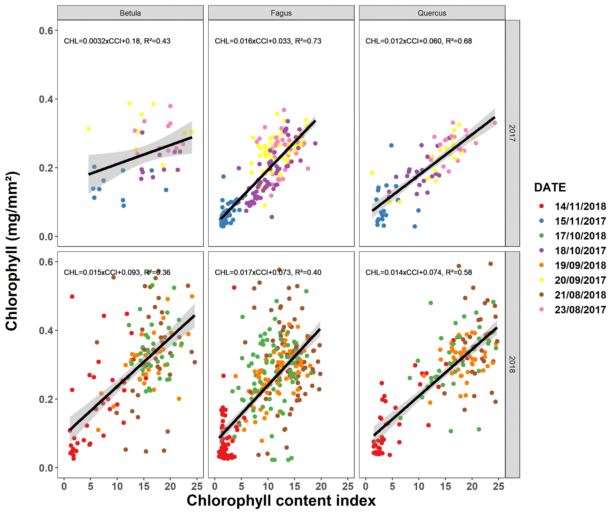
Figure A1 Relationship between the chlorophyll content index measured using a chlorophyll content meter (CCM-200 plus, Opti-Sciences Inc., Hudson, NH, USA) and the chlorophyll concentration measured using spectrophotometric analysis (Mariën et al., 2019). Between late August and late November 2017–2018, we sampled 20–40 leaves (5 leaves each for four to eight trees) for beech and 10–20 leaves (5 each for two to four trees) for birch and oak every month. The different colors represent different sampling dates.

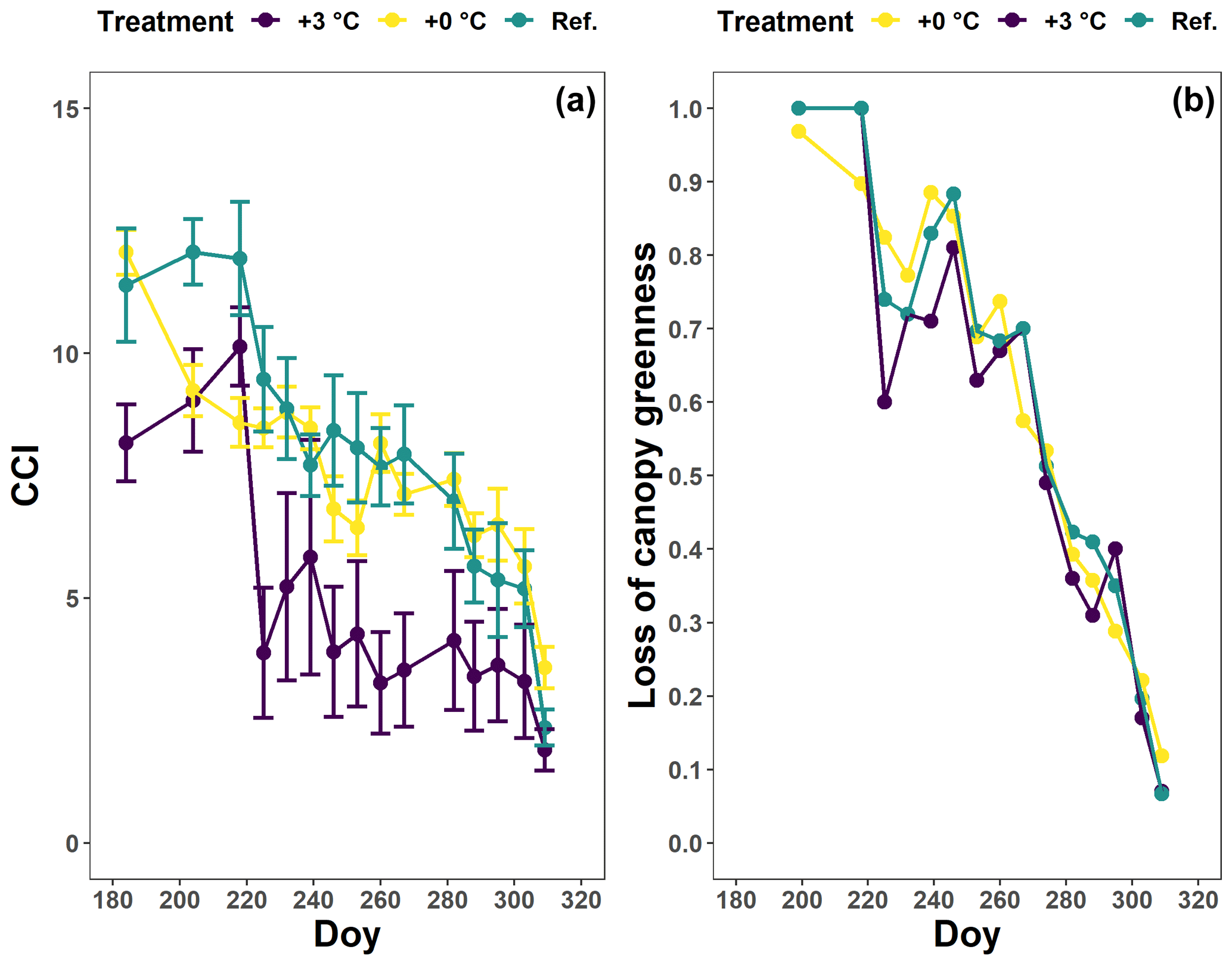
Figure A2 The chlorophyll content index (CCI; a) and loss of canopy greenness (b) of the Fagus sylvatica saplings at the Drie Eiken Campus in Wilrijk for which no breakpoint could be calculated. The dots and error bars represent the mean CCI (a) and mean loss of canopy greenness (b) with standard errors. The colors represent the CCI or the loss of canopy greenness of the beech saplings in the reference plots (green; Ref.), the glasshouses that followed the outside ambient air temperature (yellow; +0 ^∘C) and the glasshouses that were 3 ^∘C warmer than the outside ambient air temperature (purple; +3 ^∘C).

Figure A3 The mean onset of autumn leaf senescence per treatment for all Fagus sylvatica saplings at the Drie Eiken Campus in Wilrijk. Black dots represent the mean onset of autumn leaf senescence, while the error bars represent standard errors that indicate the inter-individual variability. All breakpoints are calculated using the chlorophyll content index data and piecewise linear regressions ($n_{\mathrm{Ref}.}=\mathrm{29}$; $n_{+\mathrm{0}{}^{\circ }\mathrm{C}}=\mathrm{26}$; $n_{+\mathrm{3}{}^{\circ }\mathrm{C}}=\mathrm{22}$): Ref. represents the breakpoints of the trees in the reference plots, while +0 and +3 ^∘C represent the breakpoints of the trees in the glasshouses under the less irrigation or drought and the less irrigation or drought, warming, and increased atmospheric aridity treatments, respectively.

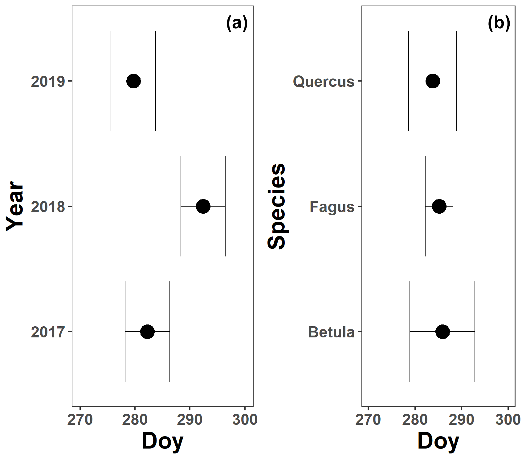
Figure A4 The mean onset of autumn leaf senescence for 3 years (a; 2017–2019) and the three species (b; Fagus sylvatica, Betula pendula and Quercus robur) measured on all mature trees at the Klein Schietveld and Park of Brasschaat. Black dots represent the mean onset of autumn leaf senescence, while the error bars represent standard errors that indicate the inter-individual variability. All breakpoints are calculated using the chlorophyll content index data and piecewise linear regressions (n_Fagus=8; n_Betula=4; n_Quercus=4).

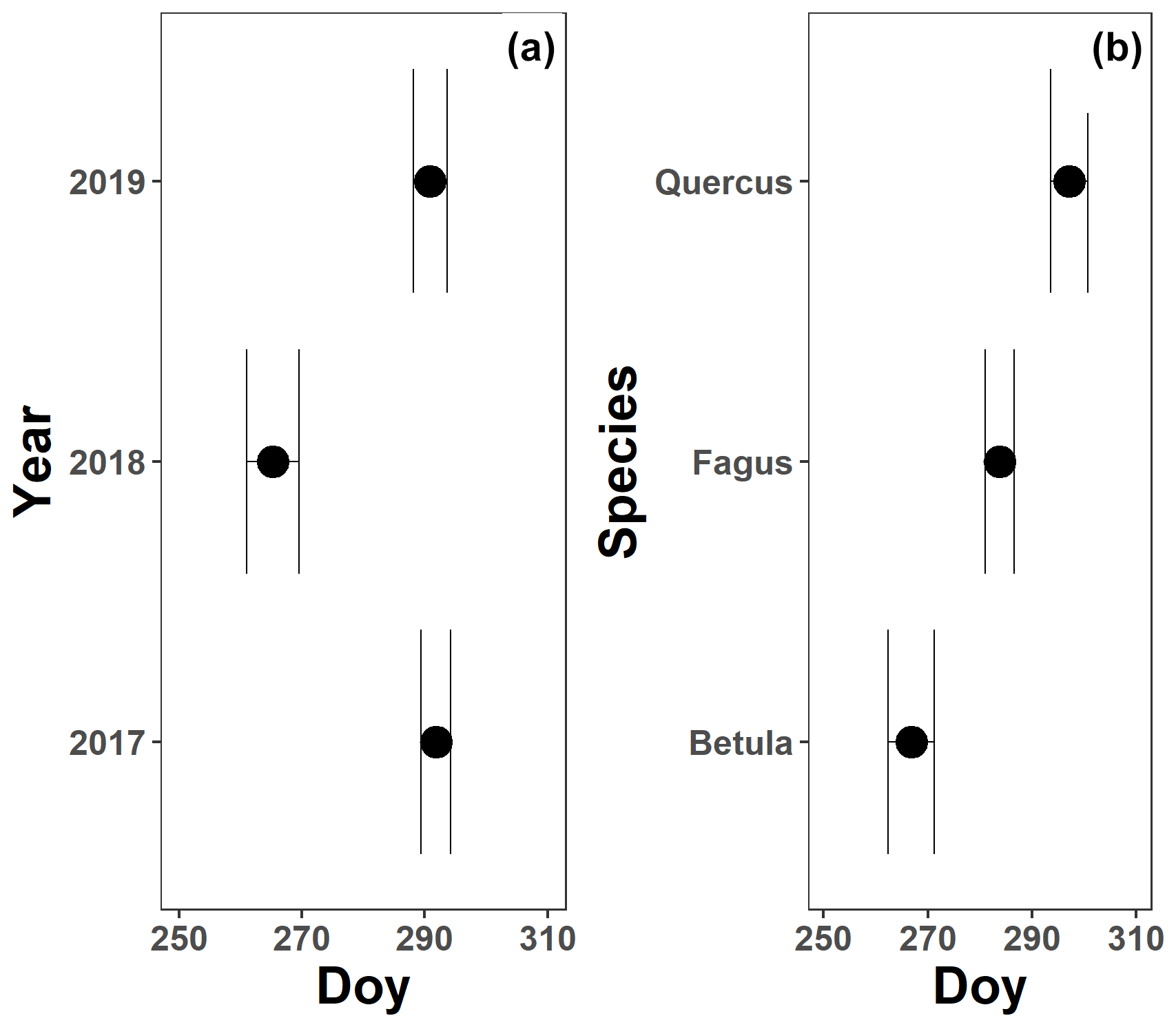
Figure A5 The mean onset of the loss of canopy greenness for 3 years (a; 2017–2019) and the three species (b; Fagus sylvatica, Betula pendula and Quercus robur) measured on all mature trees at the Klein Schietveld and Park of Brasschaat. Black dots represent the mean onset of the loss of canopy greenness, while the error bars represent standard errors that indicate the inter-individual variability. All breakpoints are calculated using the loss of canopy greenness data and piecewise linear regressions (n_Fagus=16; n_Betula=8; n_Quercus=8).