the Creative Commons Attribution 4.0 License.
the Creative Commons Attribution 4.0 License.
 | 06 Jul 2021
High-resolution induced polarization imaging of biogeochemical carbon turnover hotspots in a peatland
Timea Katona
Benjamin Silas Gilfedder
Sven Frei
Matthias Bücker
Adrian Flores-Orozco
Biogeochemical hotspots are defined as areas where biogeochemical processes occur with anomalously high reaction rates relative to their surroundings. Due to their importance in carbon and nutrient cycling, the characterization of hotspots is critical for predicting carbon budgets accurately in the context of climate change. However, biogeochemical hotspots are difficult to identify in the environment, as methods for in situ measurements often directly affect the sensitive redox-chemical conditions. Here, we present imaging results of a geophysical survey using the non-invasive induced polarization (IP) method to identify biogeochemical hotspots of carbon turnover in a minerotrophic wetland. To interpret the field-scale IP signatures, geochemical analyses were performed on freeze-core samples obtained in areas characterized by anomalously high and low IP responses. Our results reveal large variations in the electrical response, with the highest IP phase values (> 18 mrad) corresponding to high concentrations of phosphates (> 4000 µM), an indicator of carbon turnover. Furthermore, we found a strong relationship between the electrical properties resolved in IP images and the dissolved organic carbon. Moreover, analysis of the freeze core reveals negligible concentrations of iron sulfides. The extensive geochemical and geophysical data presented in our study demonstrate that IP images can track small-scale changes in the biogeochemical activity in peat and can be used to identify hotspots.
- Article
(6810 KB) - Full-text XML
- BibTeX
- EndNote


In terrestrial and aquatic ecosystems, patches or areas that show disproportionally high biogeochemical reaction rates relative to the surrounding matrix are referred to as biogeochemical “hot spots” (McClain et al., 2003). Hotspots for turnover of redox-sensitive species (e.g., oxygen, nitrate, or dissolved organic carbon) are often generated at interfaces between oxic and anoxic environments, where the local presence/absence of oxygen either favors or suppresses biogeochemical reactions such as aerobic respiration, denitrification, or oxidation/reduction of iron (McClain et al., 2003). Biogeochemical hotspots are important for nutrient and carbon cycling in various systems such as wetlands (Frei et al., 2010, 2012), lake sediments (Urban, 1994), the vadose zone (Hansen et al., 2014), hyporheic areas (Boano et al., 2014), or aquifers (Gu et al., 1998). Wetlands are distinct elements in the landscape, which are often located where hydrological flow paths converge, such as at the bottoms of basin-shaped catchments, local depressions, or around rivers and streams (Cirmo and McDonell, 1997). Wetlands are attracting increasing interest because of their important contribution to water supply, water quality, nutrient cycling, and biodiversity (Costanza et al., 1997, 2017). Understanding microbial-moderated cycling of nutrients and carbon in wetlands is critical, as these systems store a significant part of the global carbon through the accumulation of decomposed plant material (Kayranli et al., 2010). In wetlands, water table fluctuations as well as plant roots determine the vertical and horizontal distributions of oxic and anoxic areas (Frei et al., 2012; Gutknecht et al., 2006). Small-scale subsurface flow processes in wetlands, moderated by micro-topographical structures (hollow and hummocks) (Diamond et al., 2020), can control the spatial presence of redox-sensitive solutes and formation of biogeochemical hotspots (Frei et al., 2010, 2012). Despite their relevance for the carbon and nutrient cycling, basic mechanisms controlling the formation and distribution of biogeochemical hotspots in space are not well understood.
Biogeochemically active areas traditionally have been identified and localized through chemical analyses of point samples from the subsurface and subsequent interpolation of the data in space (Morse et al., 2014; Capps and Flecker, 2013; Hartley and Schlesinger, 2000). However, such point-based sampling methods may either miss hotspots due to the low spatial resolution of sampling (McClain et al., 2003) or disturb the redox-sensitive conditions in the subsurface by bringing oxygen into anoxic areas during sampling. Non-invasive methods, such as geophysical techniques, have the potential to study subsurface biogeochemical activity in situ without interfering with the subsurface environment (e.g., Williams et al., 2005, 2009; Atekwana and Slater, 2009; Flores Orozco et al., 2015, 2019, 2020). Geophysical methods permit us to map large areas in 3D and still resolve subsurface physical properties with a high spatial resolution (Binley et al., 2015).
In particular, the induced polarization (IP) technique has recently emerged as a useful tool to delineate biogeochemical processes in the subsurface (e.g., Kemna et al., 2012; Kessouri et al., 2019; Flores Orozco et al., 2020). The IP method provides information about the electrical conductivity and the capacitive properties of the ground, which can be expressed, respectively, in terms of the real and imaginary components of the complex resistivity (Binley and Kemna, 2005). The method is commonly used to explore metallic ores because of the strong polarization response associated with metallic minerals (e.g., Marshall and Madden, 1959; Seigel et al., 2007). Pelton et al. (1978) and Wong (1979) proposed the first models linking the IP response to the size and content of metallic minerals. More recently, the role of chemical and textural properties in the polarization of metallic minerals has been investigated in detail based on further developments of Wong's model of a perfect conductor and reaction currents (Bücker et al., 2018, 2019), while Revil et al. (2012, 2015a, b, 2017b, c, 2018) have presented a new mechanistic model that takes into account the intragrain polarization and Feng et al. (2020) have explained the polarization of perfectly conducting particles based on a Stern-layer capacitance. The two latter groups of models do not involve reaction currents. In porous media without a significant metallic content, the IP response can be related to the polarization of the electrical double layer formed at the grain–fluid interface (e.g., Revil and Florsch, 2010; Revil, 2012). For instance, Revil et al. (2017a) carried out IP measurements on a large set of soil samples, for which they report a linear relationship between the magnitude of the polarization response and the cation exchange capacity (CEC) which is related to surface area and surface charge density.
Since the early 2010s, various studies have explored the potential of IP measurement for the investigation of biogeochemical processes in the emerging field of biogeophysics (Slater and Attekwana, 2013). Laboratory studies on sediment samples examined the correlation between the spectral-induced polarization (SIP) response and iron sulfide precipitation caused by iron-reducing bacteria (Williams et al., 2005; Ntarlagiannis et al., 2005, 2010; Slater et al., 2007; Personna et al., 2008; Zhang et al., 2010; Placencia Gomez et al., 2013; Abdel Aal et al., 2014). Further investigations in the laboratory have also revealed an increase in the polarization response accompanying the accumulation of microbial cells and biofilms (Davis et al., 2006; Abdel Aal et al., 2010a, b; Albrecht et al., 2011; Revil et al., 2012; Zhang et al., 2013; Mellage et al., 2018; Rosier et al., 2019; Kessouri et al., 2019).
Motivated by these observations, the IP method has also been used to characterize biogeochemical degradation of contaminants at the field scale (Williams et al., 2009; Flores Orozco et al., 2011, 2012b, 2013, 2015; Maurya et al., 2017). Additionally, Wainwright et al. (2016) demonstrated the applicability of the IP imaging method to identify naturally reduced zones, i.e., hotspots, at the floodplain scale. These authors show that the accumulation of organic matter in areas with indigenous iron-reducing bacteria results in naturally reduced zones and the accumulation of iron sulfide minerals, which are classical IP targets. In line with this argumentation, Abdel Aal and Atekwana (2014) argued that the biogeochemical precipitation of iron sulfides controls the high electrical conductivity and IP response observed in hydrocarbon-impacted sites. Nonetheless, in a recent study, Flores Orozco et al. (2020) demonstrated the possibility of delineating biogeochemically active zones in a municipal solid waste landfill even in the absence of iron sulfides. Flores Orozco et al. (2020) argued that the high content of organic matter itself might explain both the high polarization response and high rates of microbial activity, thus opening up the possibility of delineating biogeochemical hotspots that are not related to iron-reducing bacteria. This conclusion is consistent with previous studies performed in marsh and peat soils, areas with a high organic matter content and high microbial turnover rates (Mansoor and Slater, 2007; McAnallen et al., 2018). Peat soils are characterized by a high surface charge and have been suggested to enhance the IP response (Slater and Reeve, 2002). Mansoor and Slater (2007) concluded that the IP method is a useful tool to map iron cycling and microbial activity in marsh soils. Garcia-Artigas et al. (2020) demonstrated that bioclogging by bacteria increases the IP response accompanying wetland treatment. Uhlemann et al. (2016) found differences in the electrical resistivity of peat according to saturation, microbial activity, and porewater conductivity; however, their study was limited to direct-current resistivity and did not investigate variations in the IP response. In contrast to these observations, laboratory studies have shown a low polarization response in samples with a high organic matter content, despite its high CEC (Schwartz and Furman, 2014). Based on field measurements, McAnallen et al. (2018) found that active peat is less polarizable due to variations in groundwater chemistry imposed by sphagnum mosses, while degrading peat resulted in low resistivity values and a high polarization response. Based on measurements with the Fourier transform infrared (FTIR) spectroscopy in water samples, the authors concluded that the carbon–oxygen (C=O) double bond in degrading peat correlated with the polarization magnitude of the peat material. Based on laboratory investigations, Ponziani et al. (2011) also concluded that decomposition of peat occurs predominantly by aerobic respiration, i.e., using molecular oxygen as the terminal electron acceptor to oxidize organic matter. Thus decomposition rates are expected to be highest at the interface between the oxic and anoxic zones.
Based on these promising previous results, we hypothesize that the IP method is a potentially useful tool for in situ investigation of biogeochemical processes and the mapping of biogeochemical hotspots. However, different responses observed in lab and field investigations do not offer a clear interpretation scheme of general validity. Additionally, it is not clear whether the IP method is only suited to characterizing biogeochemical hotspots associated with iron-reducing bacteria, which favor the accumulation of iron sulfides. Hence, in this study we present an extensive IP imaging data set collected at a peatland site to investigate the controls on the IP response in biogeochemically active areas. IP monitoring results are compared to geochemical data obtained from the analysis of freeze cores and porewater samples. Our main objectives are (i) to assess the applicability of the IP method to spatially delimit highly active biogeochemical areas in the peat soil and (ii) to investigate whether the local IP response is related to the accumulation of iron sulfides or high organic matter turnover.
2.1 Study site
The study site is part of the Lehstenbach catchment located in the Fichtelgebirge mountains (Fig. 1a), a low mountain range in northeastern Bavaria (Germany) close to the border with the Czech Republic. Various soil types including Dystric Cambisols, Haplic Podsols, and Histosols (i.e., peat soil) cover the catchment area of approximately 4.2 km2, situated on top of variscan granite bedrock (Strohmeier et al., 2013). The catchment is bowl shaped (Fig. 1b), and minerotrophic riparian peatlands have developed around the major streams. The plot-scale study site (Fig. 1c) is located in a riparian peatland draining into a nearby stream close to the catchment's outlet (Fig. 1b).
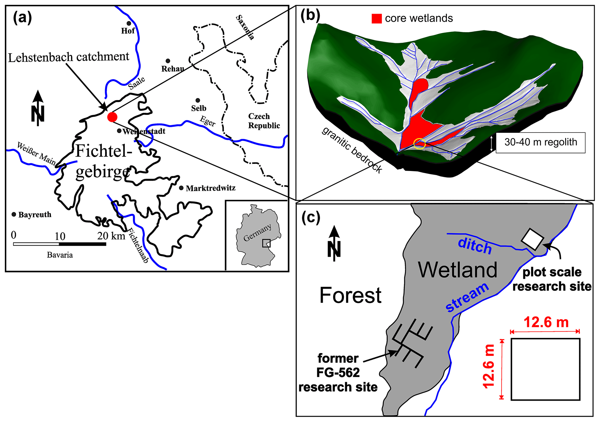
Figure 1(a) General overview of the experimental plot located in the Fichtel Mountains and (b) structure of the bowl-shaped Lehstenbach catchment and (c) location of the experimental plot.
The groundwater level in this area annually varies within the top 30 cm of the peat soil, and the local groundwater flow has a S–SW orientation (Durejka et al., 2019) towards a nearby drainage ditch. Permanently high water saturation of the peat soil favors the development of anoxic biogeochemical processes close to the surface. Frei et al. (2012) suggested that hotspots in the study area are related to the stimulation of iron-reducing bacteria and accumulation of iron sulfides, which are generated by small-scale subsurface flow processes and the spatially non-uniform availability of electron acceptors and donors induced by the typical micro-topography of the peatland. Non-uniform availability of electron acceptors and donors in combination with labile carbon stocks is the primary driver in generating biogeochemical hotspots in the peatland (Frei et al., 2012; Mishra and Riley, 2015).
2.2 Experimental plot and geochemical measurements
The experimental plot for the geophysical measurements covers approximately 160 m2 (12.6 × 12.6 m, Fig. 1c) of the riparian peatland. Sphagnum Sp. (peat moss) and Molinia caerulea (purple moor grass) dominate the vegetation, with the sphagnum and purple moor-grass abundance being higher in the northern part of the plot (Fig. 2a and b). In the southeastern region, where the sphagnum is less abundant, permanent surface runoff was observed (Fig. 2d). Peat thickness was measured with a 1 m resolution in the E–W direction and 0.5 m resolution in the N–S direction (along the IP profiles described below). To measure the thickness of the peat, a stainless-steel rod (0.5 cm in diameter) was pushed into the ground until it reached the granitic bedrock (similarly to Parry et al., 2014). The local groundwater level was measured in two piezometers and was found at ∼ 5–8 cm below the surface during the IP survey. Groundwater samples were collected at three different locations (S1, S2, and S3 indicated in Fig. 3) using a bailer. Porewater profiles were taken at S1, S2, and S3 at 5 cm intervals to a maximum depth of 50 cm below ground surface (b.g.s.) using stainless-steel mini-piezometers. All water samples were filtered through 0.45 µm filters and analyzed for fluoride, chloride, nitrite, bromide, nitrate, phosphate, and sulfate using an ion chromatograph (Compact IC plus 882, Metrohm GMBH). Dissolved organic carbon (DOC) was measured using a Shimadsu TOC analyzer via thermal combustion. Dissolved iron species (Fe2+) and total iron (Fetot) concentrations were measured photometrically using the 1,10-phenanthroline method on porewater samples that had been stabilized with 1 % vol vol 1 M HCl in the field (Tamura et al., 1974). Two freeze cores (see Fig. 2d) were extracted at locations S1 and S2 (Fig. 3) by pushing an 80 cm long stainless-steel tube into the peat. After the tube was installed, it was filled with a mixture of dry ice and ethanol. After around 20 min, the pipe with the frozen peat sample was extracted and stored on dry ice for transportation to the laboratory at the University of Bayreuth. Both freeze cores were cut into 10 cm segments. Each segment was analyzed for reactive iron (1 M HCl extraction and measured for Fetot as described above) (Canfield, 1989), reduced sulfur species using the total reduced inorganic sulfur (TRIS) method (Canfield et al., 1986) and carbon and nitrogen concentrations after combustion using a thermal conductivity detector. Peat samples were also analyzed by FTIR using a Vector 22 FTIR spectrometer (Bruker, Germany) in absorption mode with subsequent baseline subtraction on KBr pellets (200 mg dried KBr and 2 mg sample). Thirty-two measurements were recorded per sample and averaged from 4500 to 600 cm−1 in a similar manner to Biester et al. (2014).

Figure 2(a) Panoramic overview of the study site and the measurement setup. Pictures show the experimental setup and differences in the vegetation density between the northern and southern parts of the experimental plot. The induced polarization (IP) lines appear distorted due to the panoramic view. (b) Sphagnum in the northern part of the experimental plot. (c) Coaxial cables and stainless-steel electrodes used for IP measurements. (d) Vegetation and the coaxial cable bundle used for IP measurements in the water-covered area in the southeastern part of the experimental plot. (e) The freeze core shows the internal structure of the peat.
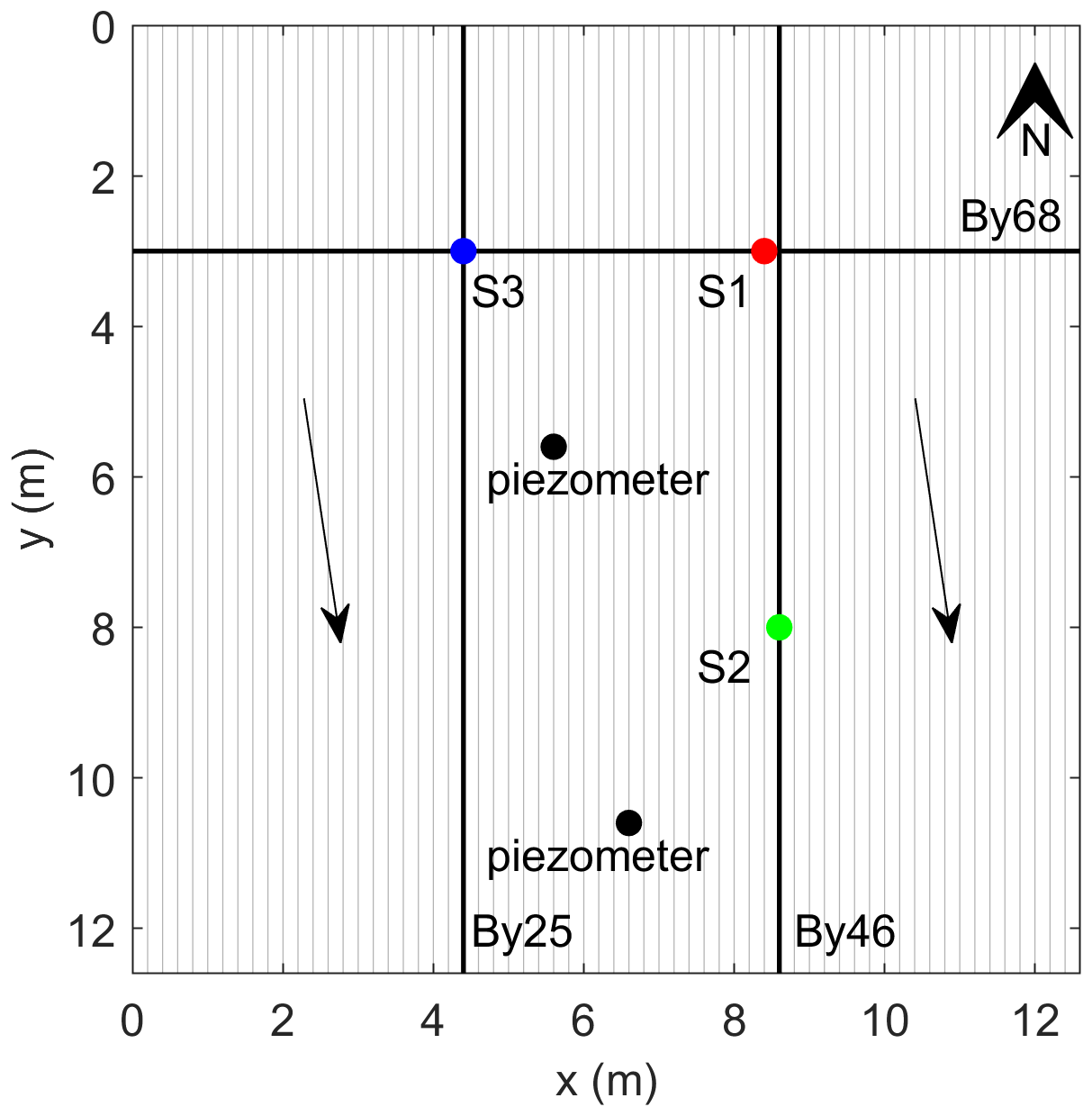
Figure 3Schematic map of the experimental plot. The solid lines represent the measured profiles; the bold lines represent the position of the profiles discussed in this paper (By 25, By 46, and By 68). The arrows indicate the groundwater flow direction. The points represent the locations of fluid (S1, S2, and S3) and freeze-core (S1, S2) samples as well as the position of piezometric tubes, where the water level was measured.
2.3 Non-invasive techniques: induced polarization measurements
The induced polarization (IP) imaging method, also known as complex conductivity imaging or electrical impedance tomography, is an extension of the electrical resistivity tomography (ERT) method (e.g., Kemna et al., 2012). As such, it is based on four-electrode measurements, where one pair of electrodes is used to inject a current (current dipole) and a second pair of electrodes is used to measure the resulting electrical potential (potential dipole). Modern devices can measure tens of potential dipoles simultaneously for a given current dipole, permitting the collection of dense data sets within a reasonable measuring time. This provides an imaging framework to gain information about lateral and vertical changes in the electrical properties of the subsurface. IP data can be collected in the frequency domain (FD), where an alternating current is injected into the ground where the polarization of the ground leads to a measurable phase shift between the injected periodic current and the measured voltage signals. From the ratio of the magnitudes of the measured voltage and the injected current as well as the phase shift between the two signals, we can obtain the electrical transfer impedance. The inversion of imaging data sets, i.e., a large set of such four-point transfer-impedance measurements collected at different locations and with different spacing between electrodes along a profile, permits us to solve for the spatial distribution of the electrical properties in the subsurface (see deGroot-Hedlin and Constable, 1990; Kemna et al., 2000; Binley and Kemna, 2005).
IP inversion results can be expressed in terms of the complex conductivity (σ*) or its inverse the complex resistivity (). The complex conductivity can be denoted either in terms of its real (σ′) and imaginary (σ′′) components or in terms of its magnitude () and phase (ϕ):
where is the imaginary unit, , and . The real part of the complex conductivity is mainly related to the Ohmic conduction, while the imaginary part is mainly related to the polarization of the subsurface materials. The conductivity (σ′) is related to porosity, saturation, the conductivity of the fluid filling the pores, and a contribution of the surface conductivity (Lesmes and Frye, 2001). The polarization (σ′′) is only related to the surface conductivity taking place at the electrical double layer (EDL) at the grain–fluid interface. For a detailed description of the IP method, the reader is referred to the work of Ward (1988), Binley and Kemna (2005), and Binley and Slater (2020).
The strongest polarization response is observed in the presence of electrically conducting minerals (e.g., iron) (e.g., Pelton et al., 1978) in the so-called electrode polarization (Wong et al., 1979). It arises from the different charge transport mechanisms in the electrical conductor (electronic or semiconductor conductivity) and the electrolytic conductivity of the surrounding pore fluid, which make the solid–liquid interface polarizable. Diffusion-controlled charging and relaxation processes inside the grain (e.g., Revil et al., 2018, 2019; Abdulsamad et al., 2019) or outside the grain in the electrolyte (e.g., Wong, 1979; Bücker et al., 2019) are considered possible causes of the polarization response at low frequencies irrespective of the specific modeling approach. All mechanistic models predict an increase in the polarization response with increasing volume content of the conductive minerals (Wong, 1979; Revil et al., 2015a, b, 2017a, b, 2018; Qi et al., 2018; Bücker et al., 2018).
In the absence of electron conductors, the polarization response is only related to the accumulation and polarization of ions in the EDL. Different models have been proposed to describe the polarization response as a function of grain size, surface area, and surface charge (e.g., Schwarz, 1962; Schurr, 1964; Leroy et al., 2008). Alternatively, the membrane polarization related the IP response to variations in the geometry of the pores as well as the concentration and mobility of the ions (e.g., Marshall and Madden, 1959; Bücker and Hördt, 2013; Bücker et al., 2019). Regardless of the specific modeling approach, EDL polarization mechanisms strongly depend on the specific surface area of the material and the charge density at the surface (Revil, 2012; Waxman and Smits, 1968).
In this study, we conducted FDIP measurements at 1 Hz along 65 lines during a period of 4 d in July 2019. We used the DAS-1 instrument manufactured by Multi-Phase Technologies (now MTP-IRIS Inc.). We collected 64 N–S-oriented lines (referred to as By 1 to By 64) with 20 cm spacing between each line. One additional line (By 68) was collected with a W–E orientation, which intersects the N–S-oriented lines at 3 m, as presented in Fig. 3. Each profile consisted of 64 stainless-steel electrodes (3 mm diameter) with a separation of 20 cm between each electrode (Fig. 2c). Besides the short electrode spacing, the use of a dipole–dipole configuration with a unit dipole length of 20 cm warranted a high resolution within the upper 50 cm of the peat, where the biogeochemical hotspots were expected. We deployed a dipole–dipole skip-0 (i.e., the dipole length for each measurement is equal to the unit spacing of 20 cm) configuration; voltage measurements were collected across eight adjacent potential dipoles for each current dipole. The dipole–dipole configuration avoids the use of electrodes for potential measurements previously used for current injections to avoid contamination of the data caused by remnant polarization of electrodes. To evaluate data quality, reciprocal readings were collected along one profile every day (see, e.g., LaBrecque et al., 1996; Flores Orozco et al., 2012a, 2019). Reciprocal readings refer to data collected after interchanging current and potential dipoles. We used coaxial cables to connect the electrodes with the measuring device to minimize the distortion of the data due to electromagnetic coupling and cross-talking between the cables (e.g., Zimmermann et al., 2008, 2019; Flores Orozco et al., 2013), with the shields of all coaxial cables running together into one ground electrode (for further details, see Flores Orozco et al., 2021).
The principle of reciprocity asserts that normal and reciprocal readings should be the same (e.g., Slater et al., 2000). Hence, we use here the analysis of the discrepancy between normal and reciprocal readings to detect outliers and to quantify data error (LaBrecque et al., 1996; Flores Orozco et al., 2012a; Slater and Binley, 2006; Slater et al., 2000). In this study, we quantified the error parameter for each line collected as normal and reciprocal pairs (using the approach outlined by Flores Orozco et al., 2012a) and computed the average value of the error parameters for the different lines to define the error model used for the inversion of all imaging data sets.
For the inversion of the IP imaging data set, we used CRTomo, a smoothness-constrained least-squares algorithm by Kemna (2000) that allows inversion of the data to a level of confidence specified by an error model. We used the resistance and phase error models described by Kemna (2000) and Flores Orozco et al. (2012a). The resistance (R) error model is expressed as , where a is the absolute error, which dominates at small resistances (i.e., R<0), and b is the relative error, which dominates at high resistance values (LaBrecque et al., 1996; Slater et al., 2000). For the phase, the error model is also expressed as a function of the resistance s(ϕa)=cRd, where d<0 in our study due to the relatively low range in the measured resistances (see Flores Orozco et al., 2012a, for further details). If d→0, the model reduces to the constant-phase-error model (Flores Orozco et al., 2012a) with s(ϕ)=c described by Kemna (2000) and Slater and Binley (2006).
3.1 Data quality and processing
In Fig. 4, we present a modified pseudosection showing both normal (negative levels) and reciprocal (positive levels) readings in terms of apparent resistivity (ρa) and apparent phase (ϕa) for the data collected along line By 25. Plots in Fig. 4 show consistency between the normal and reciprocal readings of apparent resistivity (a) and phase (b). Figure 4c and d show the histograms of the normal–reciprocal misfits along line By 25 for both the resistance and phase (ΔR and Δϕ, respectively), which exhibit near-Gaussian distributions with low standard deviations (as expected for random noise) for both the normalized resistance (SR=0.027) and the apparent phase (Sϕ=1.1 mrad). Readings exceeding these standard deviation values were considered outliers (between 16 % and 33 % of the data at the different lines) and were removed from the data set prior to the inversion.
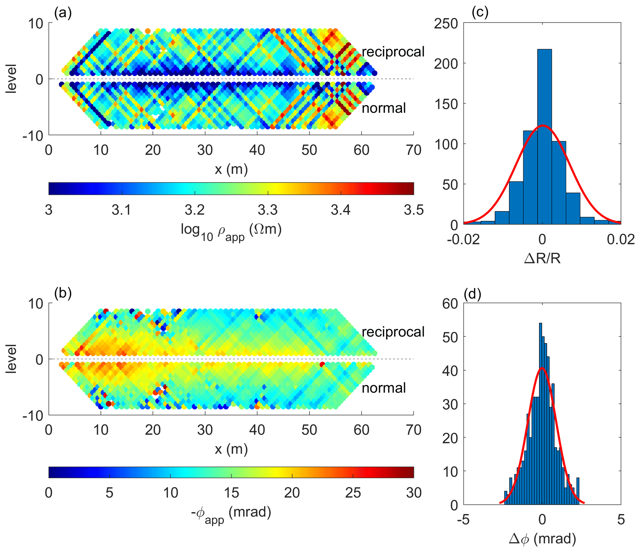
Figure 4Raw data analysis. Raw-data pseudosections of (a) the apparent resistivity and (b) the apparent phase shift for measurements collected along profile By 25. Histograms of the normal–reciprocal misfits of (c) the measured resistance (normalized) and (d) the apparent phase shift.
Here, we present inversion results obtained using the error parameters, a=0.001 Ω, b=0.022, and c=1 mrad. For the imaging, we defined a cut-off value of the cumulated sensitivity of 102.75, with pixels related to a lower cumulated sensitivity blanked in the images. The cumulated sensitivity values are a widely used parameter to assess the depth of investigation (Kemna et al., 2002; Flores Orozco et al., 2013).
3.2 Complex conductivity imaging results and their link to the peat thickness and land cover
The thickness of the peat in the plot was found to vary between 40 and 160 cm (Fig. 5). The thickness of the peat unit increased in the W–E direction, with much smaller variations in the N–S direction. Variations in the vegetation cover (as indicated by the three vegetation classes, abundant av, moderate mv, and sparse sv) do not seem to correspond to the variations in the peat thickness. Note that the N–S orientation of the majority of IP lines is approximately aligned with the direction of minimum changes in the peat thickness.
Figure 6 shows the imaging results of the N–S-oriented profiles By 25 and By 46 and the W–E-oriented profile By 68 expressed in terms of the conductivity (σ′) and polarization (σ′′). These images reveal three main electrical units: (i) a shallow peat unit with high σ′ (> 5 mSm−1) and high σ′′ (> 100 µS m−1) values in the top 10–20 cm b.g.s., (ii) an intermediate unit in the peat with moderate to low σ′ (< 5 mS m−1) and moderate σ′′ (40– 100 µS m−1) values, and, (iii) underneath it, a third unit characterized by moderate to low σ′ (< 5 mS m−1) and the lowest σ′′ (< 40 µS m−1) values corresponding to the granite bedrock. The compact structure of the granite, corresponding to low porosity, explains the observed low conductivity values (σ′ < 5 mS m−1) due to low surface charge and surface area. The shallow and intermediate electrical units are related to the relatively heterogeneous peat (Fig. 6), which is beyond the vertical change and lateral heterogeneities in the complex conductivity parameters. As shown in the plots of σ′′ in Fig. 6, the contact between the second and third units roughly corresponds to the contact between peat and granite measured with the metal rod. This indicates the ability of IP imaging to resolve the geometry of the peat unit. However, for the survey design used in this study, σ′′ images are not sensitive to materials deeper than ∼ 1.25 m. Images of the electrical conductivity reveal much more considerable variability and a lack of clear contrasts between the peat and the granite materials, likely due to the weathering of the shallow granite unit (Lischeid et al., 2002; Partington et al., 2013).
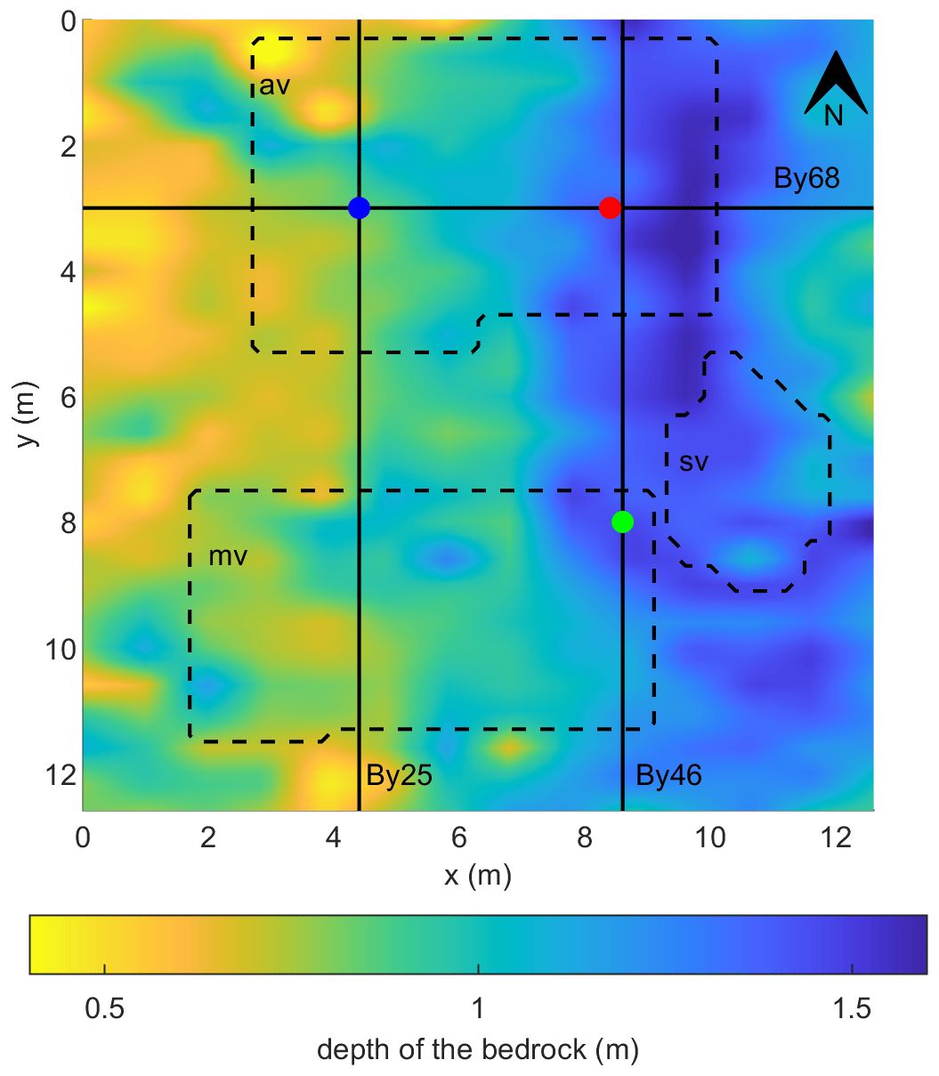
Figure 5Variations in the thickness of the peat layer, i.e., depth to the granite bedrock. The positions of the three selected IP profiles By 25, By 46, and By 68 are indicated (solid lines) as well as the position of the sampling points and the geometry of the three classes of vegetation cover: abundant vegetation (av), moderate vegetation (mv), and sparse vegetation (sv).
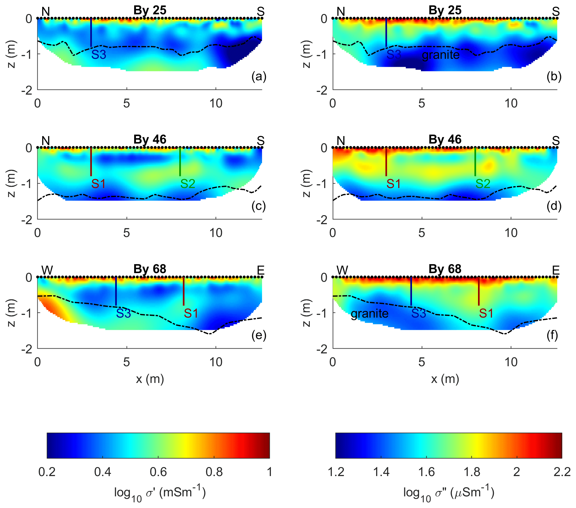
Figure 6Imaging results for data collected along profiles By 25 (a, b), By 46 (c, d), and By 68 (e, f) expressed as real σ′ and imaginary σ′′ components of the complex conductivity. The dashed lines represent the contact between the peat and granite; the black dots show the electrode positions at the surface. The vertical lines represent the locations of the fluid (S1, S2, and S3) and freeze-core (S1, S2) samples.
The phase of the complex conductivity represents the ratio of the polarization relative to the Ohmic conduction (). Thus, it can also be used to represent the polarization response (Kemna et al., 2004; Ulrich and Slater, 2004; Flores Orozco et al., 2020). Similarly to the σ′′ images, the phase images presented in Fig. 7 resolve the three main units: (i) the shallow peat unit within the top 10–50 cm is characterized by the highest values (ϕ > 18 mrad), (ii) the intermediate unit still corresponding to peat is characterized by moderate ϕ values (between 13 and 18 mrad), and (iii) the third unit, associated with the granitic bedrock, is related to the lowest ϕ values (< 13 mrad). The polarization images expressed in terms of ϕ show a higher contrast between the peat and the granite units than the σ′ (or σ′′) images. The histograms presented in Fig. 7 show the distribution of the phase values in the images, with a different color for model parameters extracted above and below the contact between peat and granite. The histograms highlight the fact that the lowest phase values clearly correspond to the granite bedrock (< 13 mrad), while higher phase values are characteristic of the peat unit.
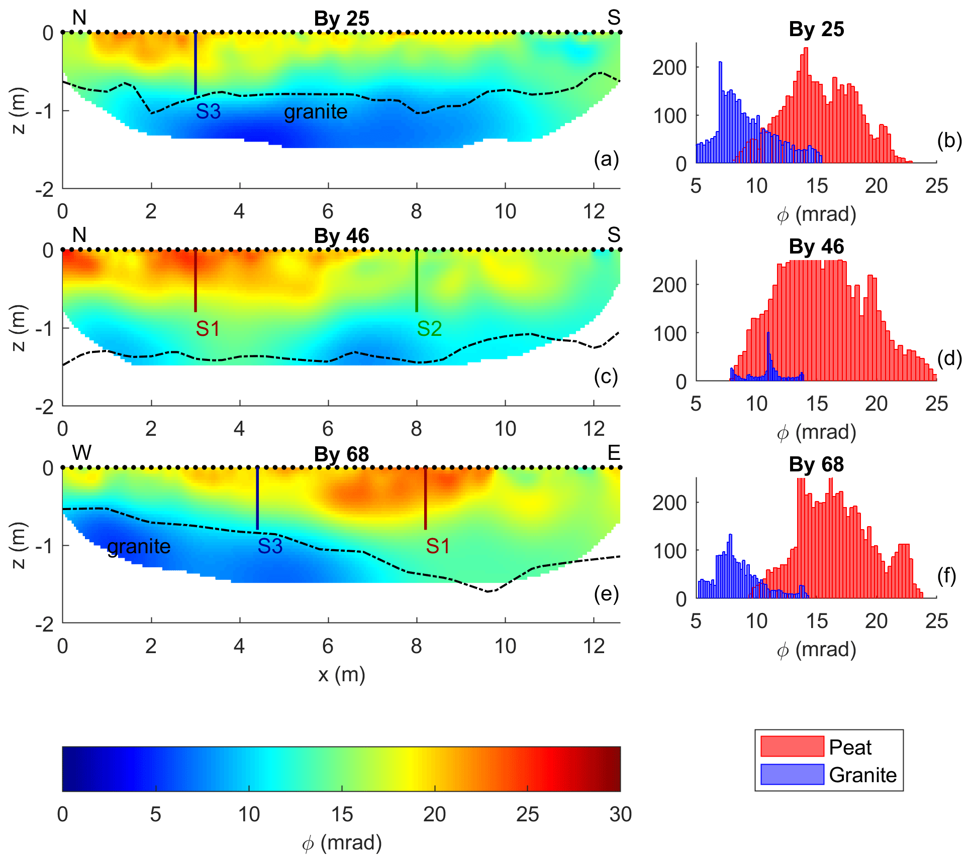
Figure 7Imaging results for data collected along profiles By 25 (a), By 46 (c), and By 68 (e), expressed as phase values ϕ of the complex conductivity. The dashed lines represent the contact between peat and granite; the black dots show the electrode positions at the surface. The vertical lines represent the location of the fluid (S1, S2, S3) and freeze-core (S1, S2) samples. The histograms represent the phase values of the granite and peat extracted from the imaging results in Fig. 6b, d, f according to the geometry of the dashed lines.
Moreover, the shallow unit shows more pronounced lateral variations in the phase than in σ′′, and patterns within the peat unit are more clearly defined. As observed in Fig. 6, along line By 25, the thickness of the first unit decreases from approx. 0.5 m at 2 m along the profile to 0 m around 10 m at the end of the profile. Along line By 46, the first unit is slightly thicker than 50 cm and shows the highest phase values (∼ 25 mrad) between 0 and 6.5 m along the profile. Beyond 6.5 m, the polarizable unit becomes discontinuous with isolated polarizable (∼ 18 mrad) zones, extending to a depth of 50 cm. The geometry of the shallow, polarizable unit is consistent with the corresponding results along line By 68, which crosses By 25 and By 46 at 3 m along these lines (S1 and S3 are located at these intersections). In particular, the highest phase values are consistently found in the shallowest 50 cm in the peat unit, at the depth where biogeochemical hotspots have been reported in the study by Frei et al. (2012).
Figure 8 presents maps of the electrical parameters at different depths aiming to identify lateral changes in the possible hotspots across the entire experimental plot. Such maps present the interpolation of values inverted in each profile. Along each profile, a value is obtained through the average of model parameters (conductivity magnitude and phase) within the surface and a depth of 20 cm (shallow maps) and between 100 and 120 cm (for deep maps). The western part of the experimental plot (between 0 and 4 m in the x direction and between 2 and 9 m in the y direction) corresponds to a shallow depth to the bedrock (a peat thickness of ∼ 50–70 cm) and is associated with high electrical parameters in the shallow maps (ϕ > 18 mrad, σ′ > 7, and σ′′ > 100 mS m−1), which we can interpret here as the geometry of the biogeochemical hotspots. Another hotspot can be identified in the northern part of the experimental plot, in the area with abundant vegetation; we observe a higher polarization response for the top 20 cm (ϕ > 18 mrad and σ′′ > 80 µS m−1) than, for instance, the one corresponding to the moderate vegetation located in the southern part. In contrast, the lowest polarization values (ϕ < 15 mrad and σ′′ < 80 µS m−1), which we interpret as biogeochemically inactive zones, are related to the area with sparse vegetation and permanent surface runoff.

Figure 8Maps of the complex conductivity at different depths. The black lines indicate the profiles By 25, By 46, and By 68. The dots represent the locations of the vertical sampling profiles S1, S2, and S3. The white lines outline areas classified as (av) abundant vegetation, (mv) moderate vegetation, (sv) sparse vegetation, and histograms of the complex-conductivity imaging results of the masked areas, the abundant vegetation (red bins), the moderate vegetation (green bins), and the sparse vegetation (blue bins).
Kleinebecker et al. (2009) suggest that besides climatic variables, biogeochemical characteristics of the peat influence the composition of vegetation in wetlands. Hence, we can use variations in the vegetation as a qualitative way of evaluating our interpretation of the IP imaging results. In Fig. 8g–i, we present the histograms of the electrical parameters extracted at each of the three vegetation features defined in the experimental plot (abundant, moderate, and sparse). These histograms show, in general, that the location with sparse vegetation, i.e., with permanent surface runoff, is related to the lowest phase values (histogram peak at 13 mrad). Moderate vegetation corresponds to moderate phase and σ′′ values (histogram peak at 18 mrad and 70 µS m−1, respectively). In comparison, the abundant vegetation corresponds to the highest phase and σ′′ values (histogram peak at 22 mrad and 90 µS m−1, respectively) in the top 20 cm. The histogram of the three vegetation features in terms of σ′ values overlaps with each other.
3.3 Comparison of electrical and geochemical parameters
The evaluations of the imaging results measured along profiles By 25, By 46, and By 68 were used to select the locations for the freeze core and sampling of groundwater. Sampling points S1 and S3 were defined in the highly polarizable parts of the uppermost peat unit (high σ′ and σ′′ values). In contrast, sampling point S2 is located in an area characterized by low polarization values. Figure 9a–e show the chemical parameters measured in the water samples, specifically chloride (Cl−), phosphate (PO), dissolved organic carbon (DOC), total iron (Fetot= Fe Fe3+), and pH, whereas Fig. 9f–j show the chemical parameters measured in the peat samples extracted from the freeze cores, namely, CEC, concentrations of iron sulfide (FeS or FeS2), total reactive iron (Fetot), potassium (K+), and sodium (Na+). The pore-fluid conductivity measured in water samples retrieved from the piezometers shows minor variation with values ranging between 6.7 and 10.4 mS m−1. To facilitate the comparison of electrical parameters and geochemical data, Fig. 9k–m show the complex conductivity parameters (σ′, σ′′, and ϕ) at the sampling points S1, S2, and S3, which were extracted as vertical 1D profiles from the corresponding imaging results.
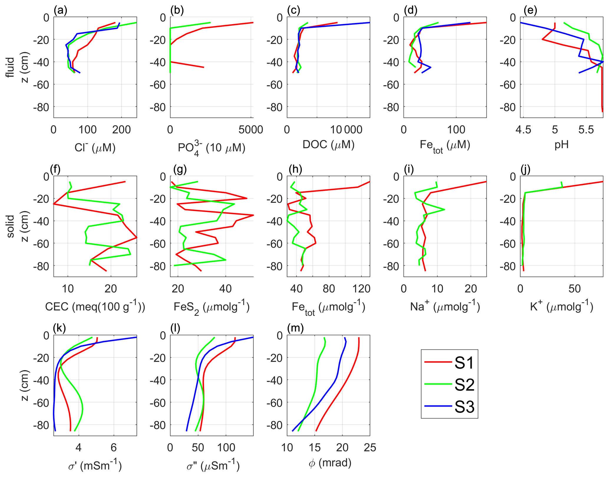
Figure 9Results of geochemical analyses of water and soil samples. Fluid-sample analysis of the (a) chloride Cl−, (b) phosphate PO, (c) dissolved organic carbon, (d) total iron Fetot, and (e) pH. Freeze-core sample analysis of the (f) cation exchange capacity CEC, (g) iron sulfide FeS2, (h) total iron Fetot, (i) sodium Na+, and (j) potassium K+. Imaging results at the three sampling locations in terms of (k) real component σ′, (l) imaginary component σ′′, and (m) phase ϕ of the complex conductivity.
As observed in Figs. 6 and 7, the highest complex conductivity values (σ′, σ′′) were resolved within the uppermost 10–20 cm and rapidly decreased with depth. Furthermore, the values of ϕ and σ′′ in the top 20 cm at S1 and S3 are significantly higher than those at location S2. High values of ϕ and σ′′ at S1 and S3 correspond to high concentrations of DOC, phosphate, Fetot in water samples, as well as high K+, and Na+ contents measured in soil materials extracted from the freeze cores. Figure 9 reveals consistent patterns between geochemical and geophysical parameters: in the first 10 cm b.g.s. close to sampling points S1 and S3, we observe complex conductivity values (σ′ and σ′′) as well as chemical parameters, such as DOC and phosphate (only at S1). Accordingly, at S1 Fetot also reveals at least 2 times higher concentrations than those measured in S2.
Figure 10 shows the actual correlations between the complex conductivity and Cl−, DOC, and Fetot concentrations measured in groundwater samples. In Fig. 10, we also provide a linear regression analysis to quantify the correlation between parameters. Figure 10 reveals that the phase has a weak to moderate correlation with DOC, Cl−, and Fetot. The conductivity (σ′) shows a slightly stronger correlation with the DOC, the Cl−, and total iron concentration than the polarization (σ′′). The highest σ′′ values (> 100 µS m−1) are related to the highest DOC and total iron concentration.
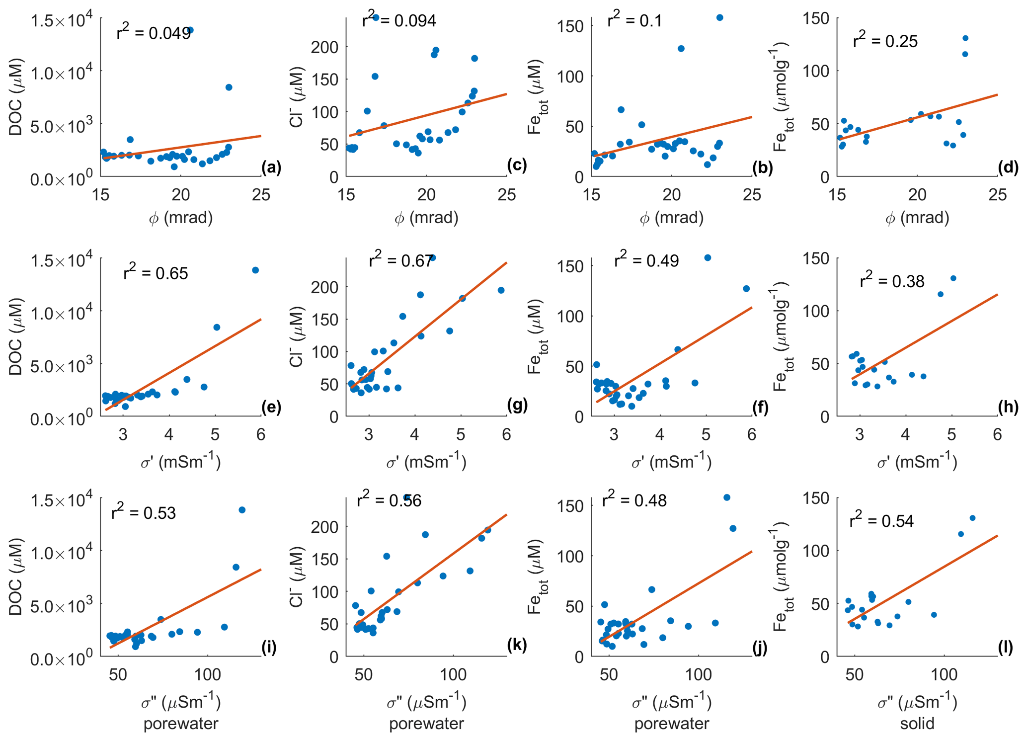
Figure 10Correlations between the geophysical and geochemical parameters, phase (ϕ), the real (σ′) and imaginary (σ′′) components of the complex conductivity (retrieved from the imaging results) and the biogeochemical analysis, expressed in terms of the dissolved organic carbon (DOC), and chloride (Cl−) content from the pore-fluid samples and total iron (Fetot) content from pore fluid in µmol L−1 and solid samples in µmol g−1. The correlation coefficients of least-square regression analysis are shown in the top left corners of the subplots.
Further evidence of the presence of the biogeochemical hotspot interpreted at the position of S1 is available by the FTIR spectroscopy analysis of the freeze-core samples presented in Fig. 11. The spectra show the absorbance intensity at different wave numbers, C–O bond (∼ 1050 cm−1), C=O double bond (∼ 1640 cm−1), carboxyl (∼ 1720 cm−1), and O–H bonds (∼ 3400 cm−1). The peaks are also indicated in Fig. 11 with the interpretation based on the typical values reported in peatlands, for instance, McAnallen et al. (2018) or Artz et al. (2008).
4.1 Biogeochemical interpretation
The geochemical and geoelectrical parameters presented in Figs. 6–7 and 9 reveal consistent patterns, with the highest values within the uppermost 10 cm around S1 and S3. The high DOC, K+, and phosphate concentrations in the uppermost peat layers and especially in the areas found to be biogeochemically active strongly suggest that there is rapid decomposition of dead plant material in these areas (Bragazza et al., 2009). Ions such as K+ and phosphate are essential plant nutrients, and phosphate species especially are often the primary limiting nutrient in peatlands (Hayati and Proctor, 1991). The presence of dissolved phosphate in porewaters suggests that (i) the plant uptake rate of this essential nutrient is exceeded by its production through the decomposition of plant material and (ii) that organic matter turnover must be rapid indeed to deliver this amount of phosphate to the porewater. This is supported by the DOC concentrations in porewater exceeding 10 mM. DOC is produced as a decomposition product during microbial hydrolysis and oxidation of solid-phase organic carbon via enzymes such as phenol oxidase (Kang et al., 2018). Enzymatic oxidation processes are enhanced by oxygen ingress via diffusion and, more importantly, by water table fluctuations that work as an “oxygen pump” to the shallow subsurface (Estop-Aragonés et al., 2012). Thus, an increased DOC concentration in the porewater can be used as an indicator of microbial activity (Elifantz et al., 2011; Liu, 2013). The small amount of phosphate measured in the less active area S2 can be explained by advective transport from the active area S1, which is directly “upstream” of S2. In this case, advective water flow through the uppermost peat layers along the hydrological head gradient may have transported a small amount of reaction products from the biogeochemical source areas to the “non-active” area. The high DOC, Fe, K+, and phosphate (only at S1) levels confirm our initial interpretation of the highly conductive and polarizable geophysical units within the first 20–50 cm b.g.s. in the surroundings of S1 and S3 as biogeochemically active areas.
The high DOC concentrations are also likely to be directly or indirectly responsible for the Fe maximum in the upper layers. Dissolved Fe was predominantly found as Fe2+ (reducing conditions), suggesting either that high labile DOC levels maintain a low redox potential or that the dissolved Fe2+ was complexed with the DOC limiting the oxidation kinetics enough so that Fe2+ can accumulate in peat porewaters. The TRIS analysis clearly showed very low levels of sulfide minerals in both freeze cores, especially in the uppermost peat layers. This was unexpected considering the reducing conditions implied by the dominance of porewater Fe2+. We argue that the lack of sulfide minerals is due to insufficient H2S or HS− needed to form FeS or FeS2 or that the redox potential was not low enough to reduce sulfate to H2S or HS−. Both mechanisms are possible, as groundwater in the catchment generally has low sulfate concentrations, and yet sulfate was detected in peat porewater samples, which would not be expected if redox potentials were low enough to reduce sulfate to sulfide. The chemical analyses do not reveal any significant or systemic vertical gradient in mineral sulfide concentrations, as expected for the site (Frei et al., 2012). The maximum in extractable (reactive) solid-phase Fe was also located in the uppermost peat layer at the “hotspot” S1. This Fe was likely in the form of iron oxides or bound to/in the plant organic matter. Such iron-rich layers typically form at the redox boundary between oxic and anoxic zones and can be highly dynamic depending on variations in the peatland water levels and oxygen ingress (Wang et al., 2017; Estop-Aragonés et al., 2013).
Similarly to other peatlands (Artz et al., 2008), the FTIR spectra show the presence of carbon–oxygen bonds such as C–O, C=O, and COOH at both S1 and S2. Furthermore, the peak intensities at S1 tend to decrease with the depth, while the peak intensities at S2 samples tend to increase in agreement with the increase in the polarization response (both phase and σ′′). This observation further supports our interpretation of the shallow 10 cm in IP images in the vicinity of S1 as a biogeochemical hotspot. However, such a biogeochemical hotspot is not related to the accumulation of iron sulfides, which was suggested by Abdel Aal and Atekwana (2014) or Wainwright et al. (2016) as the main parameter controlling the high IP response. The phosphate and Fe could potentially form complexes with the O–H groups that show an absorbance peak at 1050 cm−1 (Arai and Sparks, 2001; Parikh and Chorover, 2006). Furthermore, the iron can also form complexes with the carboxyl groups (absorbance at ∼ 1720 cm−1).
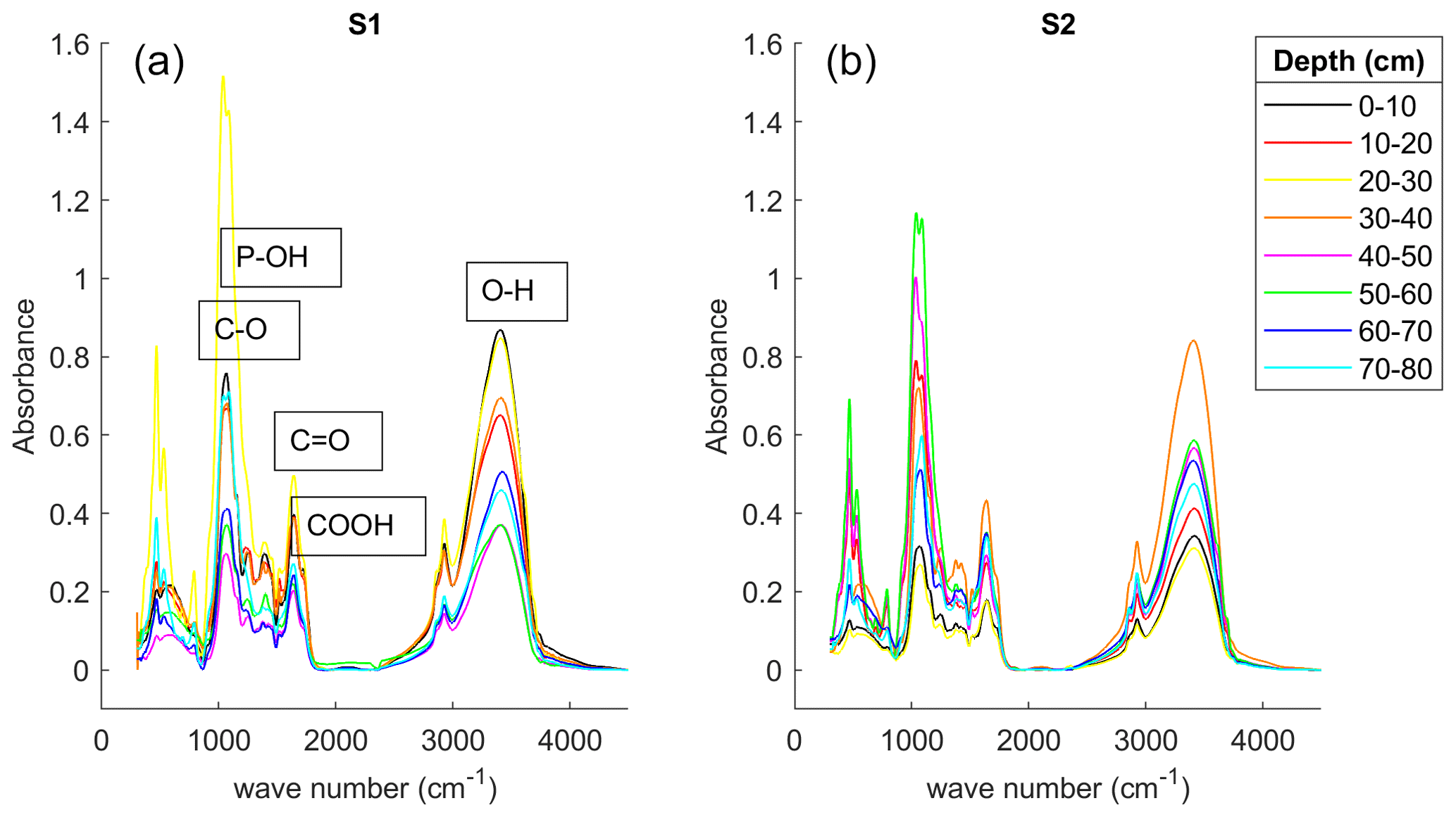
Figure 11Fourier transform infrared (FTIR) spectroscopy of the freeze-core samples collected at S1 (a) and S2 (b). Each sample was extracted from the 10 cm segments. The lines represent the depth at every 10 cm between 0 and 80 cm below the ground surface. The relevant peaks show the absorbance intensity; the interpretation is based on Artz et al. (2008), Arai and Sparks (2001), and Parikh and Chorover (2006).
4.2 Correlation between the peat and the electrical signatures
The two electrical units observed within the peat indicate variations in the biogeochemical activity with depth. Thus, it is likely that the anomalies associated with the highest σ′, σ′′, and ϕ values in the uppermost unit correspond to the location of active biogeochemical zones, i.e., a hotspot. Consequently, the moderate σ′, σ′′, and ϕ values indicate a less biogeochemically active or even inactive zone in the peat. The third unit represents the granitic bedrock. The low metal content and the well-crystallized form of the granite lead to low σ′′ values (here, < 40 µS m−1), as suggested by Marshall and Madden (1959).
The high polarization response of the biogeochemically active peat (here σ′′ > 100 µS m−1 and ϕ > 18 mrad) is consistent with the measurements of McAnallen et al. (2018), who performed time-domain IP measurements in different peatlands. They suggest that the active peat is less polarizable due to the presence of the abundant sphagnum cover. They found that in the areas where the peat is actively accumulating, the ratio of the vascular plants and the non-vascular sphagnum is low and, therefore, the oxygen availability is low. However, the sphagnum is expected to exude a small amount of carbon into the peat, and Fenner et al. (2004) found that the sphagnum contributes to the DOC leachate to the porewater, which is contradictory to the model of McAnallen et al. (2018). In agreement with Fenner et al. (2004), in our study, we also observe that high DOC content correlates with abundant sphagnum cover, which is also found in conjunction with abundant purple moor grass. In this regard, recent studies have demonstrated an increase in the polarization response due to the accumulation of biomass and activity in the root system (e.g., Weigand and Kemna 2017; Tsukanov and Schwartz, 2020). However, the sphagnum does not have roots; thus, it cannot directly contribute to the polarization response. McAnallen et al. (2018) suggest that the vascular purple moor grass can contribute to the high IP, as the roots transport oxygen into the deeper area, increasing the wettability and normalized chargeability of the peat.
Derived from the results and discussion above, we delineated the geometry of the hotspots. The map presented in Fig. 12 is based on the maps of phase and imaginary conductivity values at depths of 10 and 20 cm. Hotspots interpreted in those areas exceeded both a phase value of 18 mrad and imaginary conductivity of 100 µS m−1 at the same time. Besides the geometry of the hotspots, Fig. 12 indicates that the hotspot activity attenuates with the depth.
Figure 12Imaging results in terms of the imaginary component of the complex conductivity σ′′ > 100 µS m−1 and phase ϕ > 18 mrad, indicating the hotspot geometry at depths of (a) 10 cm and (b) 20 cm. The dots represent the locations of the vertical sampling profiles S1, S2, and S3.
4.3 Possible polarization mechanisms
In this study, we have found a strong correlation between the polarization response (ϕ and σ′′) and Fetot in the solid phase and a less pronounced correlation between the polarization response and the concentration of dissolved iron in the liquid phase (see Fig. 10). In all considered mechanistic polarization models, the phase value depends on the volumetric content of metallic particles (Wong, 1979; Revil 2015a, b; Bücker et al., 2018, 2019; Feng et al., 2020) and, therefore, the phase could reveal the possible metallic content in the peat. If the iron in the solid phase occurred in the form of highly conductive minerals, the two above correlations would point to the polarization mechanism of perfect conductors described by Wong (1979) as a possible explanation for the observed response. Previous studies (e.g., Flores Orozco et al., 2011, 2013) attributed the polarization of iron sulfides (FeS or FeS2) in sediments to such a polarization mechanism as long as sufficient Fe2+ cations are available in the porewater. Such an effect has been investigated in detail by Bücker et al. (2018, 2019) regarding the changes in the polarization response due to surface charge and reaction currents carried by redox reactions of metal ions at the mineral surface. However, in the case of the present study, the lack of sulfide and the rather high pH (inferred from the presence of sulfate) in the porewater do not favor the precipitation of conductive sulfides such as pyrite. Under these conditions, iron would rather precipitate as iron oxide or form iron–organic matter complexes. The electrical conductivity of most iron oxides is orders of magnitude smaller than the conductivity of sulfides (e.g., Cornell and Schwertmann, 1996) and is thus too low to explain an increased polarization based on a perfect-conductor polarization model (e.g., Wong, 1979; Bücker et al., 2018, 2019; Feng et al., 2020). The only highly conductive iron oxide is magnetite, with a conductivity similar to pyrite (Atekwana et al., 2016). Consequently, the presence of magnetite could explain such a polarization. However, the low pH (∼ 5) typical for peat systems does not favor the precipitation of magnetite, but rather less conducting iron (oxy)hydroxides such as ferrihydrite (Andrade et al., 2010; Linke and Gislason, 2018). Analysis of sediments of the freeze core also did not reveal magnetite. As indicated by the FTIR analysis, the iron might furthermore have built complexes with the carboxyl (absorbance at ∼ 1720 cm−1). Such moderately conductive iron minerals or iron–organic complexes might still cause a relatively strong polarization response as predicted by the polarization model developed by Revil et al. (2015) and Misra et al. (2016a). In this model, which attributes the polarization response to a diffuse intra-grain relaxation mechanism, the polarization magnitude is mainly controlled by the volumetric content. In this model, the (moderate) particle conductivity only plays a secondary role (e.g., Misra et al., 2016b).
The product of both surface charge density and specific surface area can be quantified by the CEC of a material. As peat mainly consists of organic matter known to have a high CEC, even when compared to most clay minerals (e.g., Schwartz and Furman, 2014, and references therein), the polarization of charged organic surfaces may explain the observed IP response. Additionally, Garcia-Artigas et al. (2020) concluded that bioclogging due to fine particles and biofilms increases the specific surface area and the CEC, resulting in an increase in the polarization response. However, the CEC values measured in samples retrieved from the freeze core vary in a narrow range between 5 and 25 meq kg−1, and we did not observe any correlation between CEC and changes in the polarization magnitude (σ′′, ϕ). Such a lack of correlation between the polarization effect and the CEC was also reported by Ponziani et al. (2011), who conducted spectral IP measurements on a set of peat samples. Hence, the measured CEC is high enough to explain a rise in EDL polarization; however, the (small) variation in CEC does not explain the observed variation in the polarization magnitude.
The pH of the pore fluid is also known to control the magnitude of EDL polarization; an increase in pH usually corresponds to an increase in the polarization magnitude (e.g., Skold et al., 2011). At low pH values, H+ ions occupy (negative) surface sites and thus reduce the net surface charge of the EDL (e.g., Hördt et al., 2016, and references therein). Our data seem to show the opposite behavior: we found a lower pH in the highly polarizable anomalies at S1 and S3 compared to site S2 (the inactive and less polarizable location), while the pH increases at depth for decreasing values in the polarization (both σ′′ and ϕ). At the same time, variations in pH are within the range 4.45 and 5.77 and thus might not be sufficiently large to control the observed changes in the polarization response.
Besides pH, pore-fluid salinity plays a significant role in the control of EDL polarization. Laboratory measurements on sand and sandstone samples indicated that an increase in salinity leads to an early increase in the imaginary conductivity, which is eventually followed by a peak and a decrease at very high salinities during later stages of the experiments (e.g., Revil and Skold, 2011; Weller et al., 2015). Hördt et al. (2016) provided a possible theoretical explanation for this behavior: in their membrane-polarization model, salinity controls the thickness of the diffuse layer of the EDL and depends on the specific geometry of the pores; there is an optimum thickness, which maximizes the magnitude of the polarization response. In the present study, we observed that an increase in salinity (as indicated by the high Cl− concentrations within the uppermost 10 cm at all sampling locations) is associated with an increase in the polarization magnitude response (e.g., Revil and Skold, 2011; Weller et al., 2015; Hördt et al., 2016). However, the highest Cl− concentrations were observed for the shallow layers at location S2, where we measured lower polarization magnitudes (in terms of σ′′, ϕ) compared to S1 and S3.
The strong correlation between the polarization response and the DOC suggests an, as yet not fully understood, causal relationship. A similar observation has recently been reported by Flores Orozco et al. (2020), who found a strong correlation between the organic carbon content as a proxy of microbial activity and both σ′ and σ′′ in a municipal waste landfill in Austria. Regarding the available carbon, McAnallen et al. (2018) reported a strong correlation between the occurrence of long-chained C=O double bonds and the total chargeability of peat material. The upper peat layers are exposed to oxygen, leading to oxidation of the peat and formation of C=O double bonds at solid-phase surfaces and in the porewater DOC. Such long-chained organic molecules have an increased wettability and thus more readily attach (or even form at organic matter surfaces) to the surface of solid organic and mineral particles (Alonso et al., 2009). Based on a membrane-polarization model, Bücker et al. (2017) predict an increase in the polarization magnitude in the presence of wetting (i.e., long-chained) hydrocarbon in the free phase. The long-chained polar DOC attaches to the peat surface, similarly to polar hydrocarbon, and so it might provide extra surface charge, thus reducing the pore space and causing membrane polarization (Marshall and Madden, 1959).
As suggested by Vindedahl et al. (2016), organic matter can adsorb to the iron-oxide surface via electrostatic attraction and provides a negatively charged macromolecular layer on the iron oxide. Such complexes could also explain the observed increase in the polarization response in the anomalies interpreted as biogeochemical hotspots. The point of zero charge of the peat is below pH 4 (Bakatula et al., 2018), while for iron (oxide) it varies between ∼ 5 and ∼ 9 (Kosmulski et al., 2003). This means that the organic matter is probably negatively charged, and the iron oxide is most likely positively charged since the measured pH at the sample points varies between 4.5 and 5.8, with lower values in the top 10 cm in the hotspot area. Hence, in the shallow 10 cm from S1 and S3, the pH favors the DOC to bond with the iron in the solid phase.
We investigated the applicability of induced polarization (IP) as a tool to identify and localize biogeochemically active areas or hotspots in peatlands. Although the exact polarization mechanism is not fully understood, our results reveal that the IP response of the peat changes with the level of biogeochemical activity. Thus, the IP method is capable of distinguishing between biogeochemically active and inactive zones within the peat. The phase and imaginary conductivity values show a contrast between these active and inactive zones and characterize the geometry of the hotspots even if iron sulfides are not present. The joint interpretation of chemical and geophysical data indicates that anomalous regions (characterized by phase values above 18 mrad and an imaginary conductivity of 100 µS m−1) delineate the geometry of the hotspots, which are limited to the top 10 cm b.g.s. Deeper areas (> 10 cm) of the peat are less active. In this regard, our study shows that the induced polarization method is able to characterize biogeochemical changes and their geometry within peat with high resolution. Additionally, our study demonstrates the ability of the IP method to map biogeochemically active zones even if they are not related to the microbiologically mediated accumulation of iron sulfides. We identify complexes of organic matter and iron as possible causes of the high polarization response of the carbon turnover hotspots investigated in our study. Further laboratory studies on peat samples with different concentrations and mixtures of DOC, phosphate, and iron in the pore fluid are required to fully understand the effect in IP signatures due to iron–organic complexes and the control phosphate exerts over the related polarization process.
All data are available from the corresponding author upon request.
AFO and TK designed the experimental setup, and TK conducted the field survey and analysis of the geophysical data. BSG and SF conducted the geochemical measurements and their interpretation. AFO, MB, and TK interpreted the geophysical signatures. TK lead the preparation of the draft, where SF, BSG, MB, and AFO contributed equally.
The authors declare that they have no conflict of interest.
Publisher's note: Copernicus Publications remains neutral with regard to jurisdictional claims in published maps and institutional affiliations.
This research was supported by German Research Foundation (DFG) projects FR 2858/2-1-3013594 and GI 792/2-1. The work of Timea Katona was supported by the ExploGRAF project (development of geophysical methods for the exploration of graphite ores) funded by the Austrian Federal Ministry of Science, Research and Economy. We are grateful for the constructive comments by Lee Slater and Andre Revil for improving the quality of this paper and the editorial work of Alexandra Konings.
This research has been supported by the Deutsche Forschungsgemeinschaft (grant no. 279180939).
This paper was edited by Alexandra Konings and reviewed by Andre Revil and Rutgers Newark.
Abdel Aal, G. Z. and Atekwana, E. A.: Spectral induced polarization (SIP) response of biodegraded oil in porous media, Geophys. J. Int., 196, 804–817, https://doi.org/10.1093/gji/ggt416, 2014.
Abdel Aal, G. Z., Atekwana, E. A., Rossbach, S., and Werkema, D. D.: Sensitivity of geoelectrical measurements to the presence of bacteria in porous media, J. Geophys. Res.-Biogeo., 115, G03017, https://doi.org/10.1029/2009jg001279, 2010a.
Abdel Aal, Gamal, Z., Estella, A., and Eliot, A.: Effect of bioclogging in porous media on complex conductivity signatures, J. Geophys. Res.-Biogeo., 115, G00G07, https://doi.org/10.1029/2009jg001159, 2010b.
Abdel Aal, G. Z., Atekwana, E. A., and Revil, A.: Geophysical signatures of disseminated iron minerals: A proxy for understanding subsurface biophysicochemical processes, J. Geophys. Res.-Biogeo., 119, 1831–1849, https://doi.org/10.1002/2014jg002659, 2014.
Abdulsamad, F., Revil, A., Ghorbani, A., Toy, V., Kirilova, M., Coperey, A., Duvillard, P., Ménard, G., and Ravanel, L.: Complex conductivity of graphitic schists and sandstones, J. Geophys. Res.-Sol. Ea., 124, 8223–8249, https://doi.org/10.1029/2019JB017628, 2019.
Albrecht, R., Gourry, J. C., Simonnot, M. O., and Leyval, C.: Complex conductivity response to microbial growth and biofilm formation on phenanthrene spiked medium, J. Appl. Geophys., 75, 558–564, https://doi.org/10.1016/j.jappgeo.2011.09.001, 2011.
Alonso, D. M., Granados, M. L., Mariscal, R., and Douhal, A.: Polarity of the acid chain of esters and transesterification activity of acid catalysts, J. Catal., 262, 18–26, https://doi.org/10.1016/j.jcat.2008.11.026, 2009.
Andrade, Â. L., Souza, D. M., Pereira, M. C., Fabris, J. D., and Domingues, R. Z.: pH effect on the synthesis of magnetite nanoparticles by the chemical reduction-precipitation method, Quim. Nova, 33, 524–527, https://doi.org/10.1590/s0100-40422010000300006, 2010.
Arai, Y. and Sparks, D. L.: ATR–FTIR spectroscopic investigation on phosphate adsorption mechanisms at the ferrihydrite–water interface, J. Colloid Interf. Sci., 241, 317–326, https://doi.org/10.1006/jcis.2001.7773, 2001.
Artz, R. R., Chapman, S. J., Robertson, A. J., Potts, J. M., Laggoun-Défarge, F., Gogo, S., and Francez, A. J.: FTIR spectroscopy can be used as a screening tool for organic matter quality in regenerating cutover peatlands, Soil Biol. Biochem., 40, 515–527, https://doi.org/10.1016/j.soilbio.2007.09.019, 2008.
Atekwana, E., Patrauchan, M., and Revil, A.: Induced Polarization Signature of Biofilms in Porous Media: From Laboratory Experiments to Theoretical Developments and Validation (No. DOE-Okstate-SC0007118), Oklahoma State Univ., Stillwater, OK, USA, https://doi.org/10.2172/1327843, 2016.
Atekwana, E. A. and Slater, L. D.: Biogeophysics: A new frontier in Earth science research, Rev. Geophys., 47, RG4004, https://doi.org/10.1029/2009rg000285, 2009.
Bakatula, E. N., Richard, D., Neculita, C. M., and Zagury, G. J.: Determination of point of zero charge of natural organic materials, Environ. Sci. Pollut. Res., 25, 7823–7833, https://doi.org/10.1007/s11356-017-1115-7, 2018.
Biester, H., Knorr, K. H., Schellekens, J., Basler, A., and Hermanns, Y. M.: Comparison of different methods to determine the degree of peat decomposition in peat bogs, Biogeosciences, 11, 2691–2707, https://doi.org/10.5194/bg-11-2691-2014, 2014.
Binley, A. and Kemna, A.: DC resistivity and induced polarization methods, in: Hydrogeophysics, Springer, Dordrecht, 129–156, https://doi.org/10.1007/1-4020-3102-5_5, 2005.
Binley, A. and Slater, L.: Resistivity and Induced Polarization: Theory and Applications to the Near-surface Earth, Cambridge University Press, https://doi.org/10.1017/9781108685955.003, 2020.
Binley, A., Hubbard, S. S., Huisman, J. A., Revil, A., Robinson, D. A., Singha, K., and Slater, L. D.: The emergence of hydrogeophysics for improved understanding of subsurface processes over multiple scales, Water Resour. Res., 51, 3837–3866, https://doi.org/10.1002/2015wr017016, 2015.
Boano, F., Harvey, J. W., Marion, A., Packman, A. I., Revelli, R., Ridolfi, L., and Wörman, A.: Hyporheic flow and transport processes: Mechanisms, models, and biogeochemical implications, Rev. Geophys., 52, 603–679, https://doi.org/10.1002/2012rg000417, 2014.
Bragazza, L., Buttler, A., Siegenthaler, A., and Mitchell, E. A.: Plant litter decomposition and nutrient release in peatlands, Geoph. Monog. Series, 184, 99–110, https://doi.org/10.1029/2008gm000815, 2009.
Bücker, M. and Hördt, A.: Analytical modelling of membrane polarization with explicit parametrization of pore radii and the electrical double layer, Geophys. J. Int., 194, 804–813, https://doi.org/10.1093/gji/ggt136, 2013.
Bücker, M., Orozco, A. F., Hördt, A., and Kemna, A.: An analytical membrane-polarization model to predict the complex conductivity signature of immiscible liquid hydrocarbon contaminants, Near Surf. Geophys., 15, 547–562, https://doi.org/10.3997/1873-0604.2017051, 2017.
Bücker, M., Orozco, A. F., and Kemna, A.: Electrochemical polarization around metallic particles – Part 1: The role of diffuse-layer and volume-diffusion relaxation, Geophysics, 83, E203–E217, https://doi.org/10.1190/geo2017-0401.1, 2018.
Bücker, M., Undorf, S., Flores Orozco, A., and Kemna, A.: Electrochemical polarization around metallic particles – Part 2: The role of diffuse surface charge, Geophysics, 84, E57–E73, https://doi.org/10.1190/geo2018-0150.1, 2019.
Canfield, D. E.: Reactive iron in marine sediments, Geochim. Cosmochim. Ac., 53, 619–632, https://doi.org/10.1016/0016-7037(89)90005-7, 1989.
Canfield, D. E., Raiswell, R., Westrich, J. T., Reaves, C. M., and Berner, R. A.: The use of chromium reduction in the analysis of reduced inorganic sulfur in sediments and shales, Chem. Geol., 54, 149–155, https://doi.org/10.1016/0009-2541(86)90078-1, 1986.
Capps, K. A. and Flecker, A. S.: Invasive fishes generate biogeochemical hotspots in a nutrient-limited system, PLoS One, 8, e54093, https://doi.org/10.1371/journal.pone.0054093, 2013.
Cirmo, C. P. and McDonnell, J. J.: Linking the hydrologic and biogeochemical controls of nitrogen transport in near-stream zones of temperate-forested catchments: a review, J. Hydrol., 199, 88–120, https://doi.org/10.1016/s0022-1694(96)03286-6, 1997.
Cornell, R. M. and Schwertmann, U.: The Iron Oxides, VCH, ISBN: 3-527-28567-8, 1996.
Costanza, R., d'Arge, R., De Groot, R., Farber, S., Grasso, M., Hannon, B., and Raskin, R. G.: The value of the world's ecosystem services and natural capital, Nature, 387, 253–260, https://doi.org/10.1038/387253a0, 1997.
Costanza, R., De Groot, R., Braat, L., Kubiszewski, I., Fioramonti, L., Sutton, P., and Grasso, M.: Twenty years of ecosystem services: how far have we come and how far do we still need to go?, Ecosyst. Serv., 28, 1–16, https://doi.org/10.1016/j.ecoser.2017.09.008, 2017.
Davis, C. A., Atekwana, E., Atekwana, E., Slater, L. D., Rossbach, S., and Mormile, M. R.: Microbial growth and biofilm formation in geologic media is detected with complex conductivity measurements, Geophys. Res. Lett., 33, L18403, https://doi.org/10.1029/2006gl027312, 2006.
deGroot-Hedlin, C. and Constable, S.: Occam's inversion to generate smooth, two-dimensional models from magnetotelluric data, Geophysics, 55, 1613–1624, https://doi.org/10.1190/1.1442813, 1990.
Diamond, J. S., McLaughlin, D. L., Slesak, R. A., and Stovall, A.: Microtopography is a fundamental organizing structure of vegetation and soil chemistry in black ash wetlands, Biogeosciences, 17, 901–915, https://doi.org/10.5194/bg-17-901-2020, 2020.
Durejka, S., Gilfedder, B. S., and Frei, S.: A method for long-term high resolution 222Radon measurements using a new hydrophobic capillary membrane system, J. Environ. Radioactiv., 208, 105980, https://doi.org/10.1016/j.jenvrad.2019.05.012, 2019.
Elifantz, H., Kautsky, L., Mor-Yosef, M., Tarchitzky, J., Bar-Tal, A., Chen, Y., and Minz, D.: Microbial activity and organic matter dynamics during 4 years of irrigation with treated wastewater, Microb. Ecol., 62, 973–981, https://doi.org/10.1007/s00248-011-9867-y, 2011.
Estop-Aragonés, C., Knorr, K. H., and Blodau, C.: Controls on in situ oxygen and dissolved inorganic carbon dynamics in peats of a temperate fen, J. Geophys. Res.-Biogeo., 117, G02002, https://doi.org/10.1029/2011jg001888, 2012.
Estop-Aragonés, C., Knorr, K. H., and Blodau, C.: Belowground in situ redox dynamics and methanogenesis recovery in a degraded fen during dry-wet cycles and flooding, Biogeosciences, 10, 421–436, https://doi.org/10.5194/bg-10-421-2013, 2013.
Feng, L., Li, Q., Cameron, S. D., He, K., Colby, R., Walker, K. M., and Ertaş, D.: Quantifying induced polarization of conductive inclusions in porous Media and implications for Geophysical Measurements, Sci. Rep., 10, 1–12, https://doi.org/10.1038/s41598-020-58390-z, 2020.
Fenner, N., Ostle, N., Freeman, C., Sleep, D., and Reynolds, B.: Peatland carbon efflux partitioning reveals that Sphagnum photosynthate contributes to the DOC pool, Plant Soil, 259, 345–354, https://doi.org/10.1023/b:plso.0000020981.90823.c1, 2004.
Flores Orozco, A., Williams, K. H., Long, P. E., Hubbard, S. S., and Kemna, A.: Using complex resistivity imaging to infer biogeochemical processes associated with bioremediation of an uranium-contaminated aquifer, J. Geophys. Res.-Biogeo., 116, G03001, https://doi.org/10.1029/2010jg001591, 2011.
Flores Orozco, A., Kemna, A., and Zimmermann, E.: Data error quantification in spectral induced polarization imaging, Geophysics, 77, E227–E237, https://doi.org/10.1190/geo2010-0194.1, 2012a.
Flores Orozco, A., Kemna, A., Oberdörster, C., Zschornack, L., Leven, C., Dietrich, P., and Weiss, H.: Delineation of subsurface hydrocarbon contamination at a former hydrogenation plant using spectral induced polarization imaging, J. Contam. Hydrol., 136, 131–144, https://doi.org/10.1016/j.jconhyd.2012.06.001, 2012b.
Flores Orozco, A., Williams, K. H., and Kemna, A.: Time-lapse spectral induced polarization imaging of stimulated uranium bioremediation, Near Surf. Geophys., 11, 531–544, https://doi.org/10.3997/1873-0604.2013020, 2013.
Flores Orozco, A., Velimirovic, M., Tosco, T., Kemna, A., Sapion, H., Klaas, N., and Bastiaens, L.: Monitoring the injection of microscale zerovalent iron particles for groundwater remediation by means of complex electrical conductivity imaging, Environ. Sci. Technol., 49, 5593–5600, https://doi.org/10.1021/acs.est.5b00208, 2015.
Flores Orozco, A., Kemna, A., Binley, A., and Cassiani, G.: Analysis of time-lapse data error in complex conductivity imaging to alleviate anthropogenic noise for site characterization, Geophysics, 84, B181–B193, https://doi.org/10.1190/geo2017-0755.1, 2019.
Flores Orozco, A., Gallistl, J., Steiner, M., Brandstätter, C., and Fellner, J.: Mapping biogeochemically active zones in landfills with induced polarization imaging: The Heferlbach landfill, Waste Manage., 107, 121–132, https://doi.org/10.1016/j.wasman.2020.04.001, 2020.
Flores Orozco, A., Aigner, L., and Gallistl, J.: Investigation of cable effects in spectral induced polarization imaging at the field scale using multicore and coaxial cables, Geophysics, 86, E59–E75, https://doi.org/10.1190/geo2019-0552.1, 2021.
Frei, S., Lischeid, G., and Fleckenstein, J. H.: Effects of micro-topography on surface–subsurface exchange and runoff generation in a virtual riparian wetland – A modeling study, Adv. Water Resour., 33, 1388–1401, https://doi.org/10.1016/j.advwatres.2010.07.006, 2010.
Frei, S., Knorr, K. H., Peiffer, S., and Fleckenstein, J. H.: Surface micro-topography causes hot spots of biogeochemical activity in wetland systems: A virtual modeling experiment, J. Geophys. Res.-Biogeo., 117, G00N12, https://doi.org/10.1029/2012jg002012, 2012.
Garcia-Artigas, R., Himi, M., Revil, A., Urruela, A., Lovera, R., Sendrós, A., and Rivero, L.: Time-domain induced polarization as a tool to image clogging in treatment wetlands, Sci. Total Environ., 724, 138189, https://doi.org/10.1016/j.scitotenv.2020.138189, 2020.
Gu, B., Liang, L., Dickey, M. J., Yin, X., and Dai, S.: Reductive precipitation of uranium (VI) by zero-valent iron, Environ. Sci. Technol., 32, 3366–3373, https://doi.org/10.1021/es980010o, 1998.
Gutknecht, J. L., Goodman, R. M., and Balser, T. C.: Linking soil process and microbial ecology in freshwater wetland ecosystems, Plant Soil, 289, 17–34, https://doi.org/10.1007/s11104-006-9105-4, 2006.
Hansen, D. J., McGuire, J. T., Mohanty, B. P., and Ziegler, B. A.: Evidence of aqueous iron sulfid clusters in the vadose zone, Vadose Zone J., 13, 1–12, https://doi.org/10.2136/vzj2013.07.0136, 2014.
Hartley, A. E. and Schlesinger, W. H.: Environmental controls on nitric oxide emission from northern Chihuahuan desert soils, Biogeochemistry, 50, 279–300, https://doi.org/10.1023/a:1006377832207, 2000.
Hayati, A. A. and Proctor, M. C. F.: Limiting nutrients in acid-mire vegetation: peat and plant analyses and experiments on plant responses to added nutrients, J. Ecol., 79, 75–95, https://doi.org/10.2307/2260785, 1991.
Hördt, A., Bairlein, K., Bielefeld, A., Bücker, M., Kuhn, E., Nordsiek, S., and Stebner, H.: The dependence of induced polarization on fluid salinity and pH, studied with an extended model of membrane polarization, J. Appl. Geophys., 135, 408–417, https://doi.org/10.1016/j.jappgeo.2016.02.007, 2016.
Kang, H., Kwon, M. J., Kim, S., Lee, S., Jones, T. G., Johncock, A. C., and Freeman, C.: Biologically driven DOC release from peatlands during recovery from acidification, Nat. Commun., 9, 1–7, https://doi.org/10.1038/s41467-018-06259-1, 2018.
Kayranli, B., Scholz, M., Mustafa, A., and Hedmark, Å.: Carbon storage and fluxes within freshwater wetlands: a critical review, Wetlands, 30, 111–124, https://doi.org/10.1007/s13157-009-0003-4, 2010.
Kemna, A.: Tomographic Inversion of Complex Resistivity: Theory and Application, Der Andere Verlag Osnabrück, Germany, ISBN 3-934366-92-9, 2000.
Kemna, A., Binley, A., Ramirez, A., and Daily, W.: Complex resistivity tomography for environmental applications, Chem. Eng. J., 77, 11–18, https://doi.org/10.1016/s1385-8947(99)00135-7, 2000.
Kemna, A., Vanderborght, J., Kulessa, B., and Vereecken, H.: Imaging and characterisation of subsurface solute transport using electrical resistivity tomography (ERT) and equivalent transport models, J. Hydrol., 267, 125–146, https://doi.org/10.1016/s0022-1694(02)00145-2, 2002.
Kemna, A., Binley, A., and Slater, L.: Crosshole IP imaging for engineering and environmental applications, Geophysics, 69, 97–107, https://doi.org/10.1190/1.1649379, 2004.
Kemna, A., Binley, A., Cassiani, G., Niederleithinger, E., Revil, A., Slater, L., and Kruschwitz, S.: An overview of the spectral induced polarization method for near-surface applications, Near Surf. Geophys., 10, 453–468, https://doi.org/10.3997/1873-0604.2012027, 2012.
Kessouri, P., Furman, A., Huisman, J. A., Martin, T., Mellage, A., Ntarlagiannis, D., and Kemna, A.: Induced polarization applied to biogeophysics: recent advances and future prospects, Near Surf. Geophys., 17, 595–621, https://doi.org/10.1002/nsg.12072, 2019.
Kleinebecker, T., Hölzel, N., and Vogel, A.: South Patagonian ombrotrophic bog vegetation reflects biogeochemical gradients at the landscape level, J. Veg. Sci., 19, 151–160, https://doi.org/10.3170/2008-8-18370, 2008.
Kosmulski, M., Maczka, E., Jartych, E., and Rosenholm, J. B.: Synthesis and characterization of goethite and goethite–hematite composite: experimental study and literature survey, Adv. Colloid Interfac., 103, 57–76, https://doi.org/10.1016/s0001-8686(02)00083-0, 2003.
LaBrecque, D. J., Miletto, M., Daily, W., Ramirez, A., and Owen, E.: The effects of noise on Occam's inversion of resistivity tomography data, Geophysics, 61, 538–548, https://doi.org/10.1190/1.1443980, 1996.
Leroy, P., Revil, A., Kemna, A., Cosenza, P., and Ghorbani, A.: Complex conductivity of water-saturated packs of glass beads, J. Colloid Interfac., 321, 103–117, https://doi.org/10.1016/j.jcis.2007.12.031, 2008.
Lesmes, D. P. and Frye, K. M.: Influence of pore fluid chemistry on the complex conductivity and induced polarization responses of Berea sandstone, J. Geophys. Res.-Sol. Ea., 106, 4079–4090, https://doi.org/10.1029/2000jb900392, 2001.
Linke, T. and Gislason, S. R.: Stability of iron minerals in Icelandic peat areas and transport of heavy metals and nutrients across oxidation and salinity gradients–a modelling approach, Energy Proced., 146, 30–37, https://doi.org/10.1016/j.egypro.2018.07.005, 2018.
Lischeid, G., Kolb, A., and Alewell, C.: Apparent translatory flow in groundwater recharge and runoff generation, J. Hydrol., 265, 195–211, https://doi.org/10.1016/s0022-1694(02)00108-7, 2002.
Liu, H.: Thermal response of soil microbial respiration is positively associated with labile carbon content and soil microbial activity, Geoderma, 193, 275–281, https://doi.org/10.1016/j.geoderma.2012.10.015, 2013.
Mansoor, N. and Slater, L.: On the relationship between iron concentration and induced polarization in marsh soils, Geophysics, 72, A1–A5, https://doi.org/10.1190/1.2374853, 2007.
Marshall, D. J. and Madden, T. R.: Induced polarization, a study of its causes, Geophysics, 24, 790–816, https://doi.org/10.1190/1.1438659, 1959.
Maurya, P. K., Rønde, V. K., Fiandaca, G., Balbarini, N., Auken, E., Bjerg, P. L., and Christiansen, A. V.: Detailed landfill leachate plume mapping using 2D and 3D electrical resistivity tomography-with correlation to ionic strength measured in screens, J. Appl. Geophys., 138, 1–8, https://doi.org/10.1016/j.jappgeo.2017.01.019, 2017.
McAnallen, L., Doherty, R., Donohue, S., Kirmizakis, P., and Mendonça, C.: Combined use of geophysical and geochemical methods to assess areas of active, degrading and restored blanket bog, Sci. Total Environ., 621, 762–771, https://doi.org/10.1016/j.scitotenv.2017.11.300, 2018.
McClain, M. E., Boyer, E. W., Dent, C. L., Gergel, S. E., Grimm, N. B., Groffman, P. M., and McDowell, W. H.: Biogeochemical hot spots and hot moments at the interface of terrestrial and aquatic ecosystems, Ecosystems, 6, 301–312, https://doi.org/10.1007/s10021-003-0161-9, 2003.
Mellage, A., Smeaton, C. M., Furman, A., Atekwana, E. A., Rezanezhad, F., and Van Cappellen, P.: Linking spectral induced polarization (SIP) and subsurface microbial processes: Results from sand column incubation experiments, Environ. Sci. Technol., 52, 2081–2090, https://doi.org/10.1021/acs.est.7b04420, 2018.
Mishra, U. and Riley, W. J.: Scaling impacts on environmental controls and spatial heterogeneity of soil organic carbon stocks, Biogeosciences, 12, 3993–4004, https://doi.org/10.5194/bg-12-3993-2015, 2015.
Misra, S., Torres-Verdín, C., Revil, A., Rasmus, J., and Homan, D.: Interfacial polarization of disseminated conductive minerals in absence of redox-active species – Part 1: Mechanistic model and validation, Geophysics, 81, E139–E157, https://doi.org/10.1190/geo2015-0346.1, 2016a.
Misra, S., Torres-Verdín, C., Revil, A., Rasmus, J., and Homan, D.: Interfacial polarization of disseminated conductive minerals in absence of redox-active species – Part 2: Effective electrical conductivity and dielectric permittivity Interfacial polarization due to inclusions, Geophysics, 81, E159–E176, https://doi.org/10.1190/geo2015-0400.1, 2016b.
Morse, J. L., Werner, S. F., Gillin, C. P., Goodale, C. L., Bailey, S. W., McGuire, K. J., and Groffman, P. M.: Searching for biogeochemical hot spots in three dimensions: Soil C and N cycling in hydropedologic settings in a northern hardwood forest, J. Geophys. Res.-Biogeo., 119, 1596–1607, https://doi.org/10.1002/2013jg002589, 2014.
Ntarlagiannis, D., Williams, K. H., Slater, L., and Hubbard, S.: Low-frequency electrical response to microbial induced sulfid precipitation, J. Geophys. Res.-Biogeo., 110, G02009, https://doi.org/10.1029/2005jg000024, 2005.
Ntarlagiannis, D., Doherty, R., and Williams, K. H.: Spectral induced polarization signatures of abiotic FeS precipitation SIP signatures of FeS precipitation, Geophysics, 75, F127–F133, https://doi.org/10.1190/1.3467759, 2010.
Parikh, S. J. and Chorover, J.: ATR-FTIR spectroscopy reveals bond formation during bacterial adhesion to iron oxide, Langmuir, 22, 8492–8500, https://doi.org/10.1021/la061359p, 2006.
Parry, L. E., West, L. J., Holden, J., and Chapman, P. J.: Evaluating approaches for estimating peat depth, J. Geophys. Res.-Biogeo., 119, 567–576, https://doi.org/10.1002/2013jg002411, 2014.
Partington, D., Brunner, P., Frei, S., Simmons, C. T., Werner, A. D., Therrien, R., and Fleckenstein, J. H.: Interpreting streamflow generation mechanisms from integrated surface-subsurface flow models of a riparian wetland and catchment, Water Resour. Res., 49, 5501–5519, https://doi.org/10.1002/wrcr.20405, 2013.
Pelton, W. H., Ward, S. H., Hallof, P. G., Sill, W. R., and Nelson, P. H.: Mineral discrimination and removal of inductive coupling with multifrequency IP, Geophysics, 43, 588–609, https://doi.org/10.1190/1.1440839, 1978.
Personna, Y. R., Ntarlagiannis, D., Slater, L., Yee, N., O'Brien, M., and Hubbard, S.: Spectral induced polarization and electrodic potential monitoring of microbially mediated iron sulfid transformations, J. Geophys. Res.-Biogeo., 113, G02020, https://doi.org/10.1029/2007jg000614, 2008.
Placencia-Gómez, E., Slater, L., Ntarlagiannis, D., and Binley, A.: Laboratory SIP signatures associated with oxidation of disseminated metal sulfids, J. Contam. Hydrol., 148, 25–38, https://doi.org/10.1016/j.jconhyd.2013.02.007, 2013.
Ponziani, M., Slob, E. C., Ngan-Tillard, D. J. M., and Vanhala, H.: Influence of water content on the electrical conductivity of peat, Int. Water Technol. J., 1, 14–21, 2011.
Qi, Y., Soueid Ahmed, A., Revil, A., Ghorbani, A., Abdulsamad, F., Florsch, N., and Bonnenfant, J.: Induced polarization response of porous media with metallic particles – Part 7: Detection and quantification of buried slag heaps, Geophysics, 83, E277–E291, https://doi.org/10.1190/geo2017-0760.1, 2018.
Revil, A.: Spectral induced polarization of shaly sands: Influence of the electrical double layer, Water Resour. Res., 48, W02517, https://doi.org/10.1029/2011wr011260, 2012.
Revil, A. and Florsch, N.: Determination of permeability from spectral induced polarization in granular media, Geophys. J. Int., 181, 1480–1498, https://doi.org/10.1111/j.1365-246x.2010.04573.x, 2010.
Revil, A. and Skold, M.: Salinity dependence of spectral induced polarization in sands and sandstones, Geophys. J. Int., 187, 813–824, https://doi.org/10.1111/j.1365-246x.2011.05181.x, 2011.
Revil, A., Atekwana, E., Zhang, C., Jardani, A., and Smith, S.: A new model for the spectral induced polarization signature of bacterial growth in porous media, Water Resour. Res., 48, W09545, https://doi.org/10.1029/2012wr011965, 2012.
Revil, A., Florsch, N., and Mao, D.: Induced polarization response of porous media with metallic particles – Part 1: A theory for disseminated semiconductors, Geophysics, 80, D525–D538, https://doi.org/10.1190/geo2014-0577.1, 2015a.
Revil, A., Abdel Aal, G. Z., Atekwana, E. A., Mao, D., and Florsch, N.: Induced polarization response of porous media with metallic particles – Part 2: Comparison with a broad database of experimental data, Geophysics, 80, D539–D552, https://doi.org/10.1190/geo2014-0578.1, 2015b.
Revil, A., Coperey, A., Shao, Z., Florsch, N., Fabricius, I. L., Deng, Y., and van Baaren, E. S.: Complex conductivity of soils, Water Resour. Res., 53, 7121–7147, https://doi.org/10.1002/2017wr020655, 2017a.
Revil, A., Sleevi, M. F., and Mao, D.: Induced polarization response of porous media with metallic particles – Part 5: Influence of the background polarization, Geophysics, 82, E77–E96, https://doi.org/10.1190/geo2016-0388.1, 2017b.
Revil, A., Mao, D., Shao, Z., Sleevi, M. F., and Wang, D.: Induced polarization response of porous media with metallic particles – Part 6: The case of metals and semimetals, Geophysics, 82, E97–E110, https://doi.org/10.1190/geo2016-0389.1, 2017c.
Revil, A., Coperey, A., Mao, D., Abdulsamad, F., Ghorbani, A., Rossi, M., and Gasquet, D.: Induced polarization response of porous media with metallic particles – Part 8: Influence of temperature and salinity, Geophysics, 83, E435–E456, https://doi.org/10.1190/geo2018-0089.1, 2018.
Rosier, C. L., Atekwana, E. A., Aal, G. A., and Patrauchan, M. A.: Cell concentrations and metabolites enhance the SIP response to biofilm matrix components, J. Appl. Geophys., 160, 183–194, https://doi.org/10.1016/j.jappgeo.2018.10.023, 2019.
Schurr, J. M.: On the theory of the dielectric dispersion of spherical colloidal particles in electrolyte solution1, J. Phys. Chem., 68, 2407–2413, https://doi.org/10.1021/j100791a004, 1964.
Schwartz, N. and Furman, A.: On the spectral induced polarization signature of soil organic matter, Geophys. J. Int., 200, 589–595, https://doi.org/10.1093/gji/ggu410, 2014.
Schwarz, G.: A theory of the low-frequency dielectric dispersion of colloidal particles in electrolyte solution1, 2, J. Phys. Chem., 66, 2636–2642, https://doi.org/10.1021/j100818a066, 1962.
Seigel, H., Nabighian, M., Parasnis, D. S., and Vozoff, K.: The early history of the induced polarization method, Leading Edge, 26, 312–321, https://doi.org/10.1190/1.2715054, 2007.
Skold, M., Revil, A., and Vaudelet, P.: The pH dependence of spectral induced polarization of silica sands: Experiment and modeling, Geophys. Res. Lett., 38, L12304, https://doi.org/10.1029/2011gl047748, 2011.
Slater, L. and Atekwana, E.: Geophysical signatures of subsurface microbial processes, Eos, Transactions American Geophysical Union, 94, 77–78, https://doi.org/10.1002/2013eo080001, 2013.
Slater, L. and Binley, A.: Synthetic and field-based electrical imaging of a zerovalent iron barrier: Implications for monitoring long-term barrier performance, Geophysics, 71, B129–B137, https://doi.org/10.1190/1.2235931, 2006.
Slater L. D. and Reeve A.: Investigating peatland stratigraphy and hydrogeology using integrated electrical geophysics, Geophys., 67, 365–378, https://doi.org/10.1190/1.1468597, 2002.
Slater, L., Binley, A. M., Daily, W., and Johnson, R.: Cross-hole electrical imaging of a controlled saline tracer injection, J. Appl. Geophys., 44, 85–102, https://doi.org/10.1016/s0926-9851(00)00002-1, 2000.
Slater, L., Ntarlagiannis, D., Personna, Y. R., and Hubbard, S.: Pore-scale spectral induced polarization signatures associated with FeS biomineral transformations, Geophys. Res. Lett., 34, L21404, https://doi.org/10.1029/2007gl031840, 2007.
Strohmeier, S., Knorr, K.-H., Reichert, M., Frei, S., Fleckenstein, J. H., Peiffer, S., and Matzner, E.: Concentrations and fluxes of dissolved organic carbon in runoff from a forested catchment: insights from high frequency measurements, Biogeosciences, 10, 905–916, https://doi.org/10.5194/bg-10-905-2013, 2013.
Tamura, H., Goto, K., Yotsuyanagi, T., and Nagayama, M.: Spectrophotometric determination of iron (II) with 1, 10-phenanthroline in the presence of large amounts of iron (III), Talanta, 21, 314–318, https://doi.org/10.1016/0039-9140(74)80012-3, 1974.
Tsukanov, K. and Schwartz, N.: Relationship between wheat root properties and its electrical signature using the spectral induced polarization method, Vadose Zone J., 19, e20014, https://doi.org/10.1002/vzj2.20014, 2020.
Uhlemann, S. S., Sorensen, J. P. R., House, A. R., Wilkinson, P. B., Roberts, C., Gooddy, D. C., Binley, A. M., and Chambers, J. E.: Integrated time-lapse geoelectrical imaging of wetland hydrological processes, Water Resour. Res., 52, 1607–1625, https://doi.org/10.1002/2015wr017932, 2016.
Ulrich, C. and Slater, L.: Induced polarization measurements on unsaturated, unconsolidated sands, Geophysics, 69, 762–771, https://doi.org/10.1190/1.1759462, 2004.
Urban, N. R.: Retention of sulfur in lake-sediments, in: Environmental Chemistry of Lakes and Reservoirs, edited by: Baker, L. A., Am. Chem. S., 237, 323–369, https://doi.org/10.1021/ba-1994-0237.ch010, 1994.
Vindedahl, A. M., Strehlau, J. H., Arnold, W. A., and Penn, R. L.: Organic matter and iron oxide nanoparticles: aggregation, interactions, and reactivity, Environ. Sci.-Nano, 3, 494–505, https://doi.org/10.1039/c5en00215j, 2016.
Wainwright, H. M., Flores Orozco, A., Bücker, M., Dafflon, B., Chen, J., Hubbard, S. S., and Williams, K. H.: Hierarchical Bayesian method for mapping biogeochemical hot spots using induced polarization imaging, Water Resour. Res., 52, 533–551, https://doi.org/10.1002/2015wr017763, 2016.
Wang, Y., Wang, H., He, J. S., and Feng, X.: Iron-mediated soil carbon response to water-table decline in an alpine wetland, Nat. Commun., 8, 1–9, https://doi.org/10.1038/ncomms15972, 2017.
Ward, S. H.: The resistivity and induced polarization methods, in: Symposium on the Application of Geophysics to Engineering and Environmental Problems 1988, Society of Exploration Geophysicists, 109–250, https://doi.org/10.4133/1.2921804, 1988.
Waxman, M. H. and Smits, L. J. M.: Electrical conductivities in oil-bearing shaly sands, Soc. Petrol. Eng. J., 8, 107–122, https://doi.org/10.2118/1863-a, 1968.
Weigand, M. and Kemna, A.: Multi-frequency electrical impedance tomography as a non-invasive tool to characterize and monitor crop root systems, Biogeosciences, 14, 921–939, https://doi.org/10.5194/bg-14-921-2017, 2017.
Weller, A., Zhang, Z., and Slater, L.: High-salinity polarization of sandstones, Geophysics, 80, D309–D318, https://doi.org/10.1190/geo2014-0483.1, 2015.
Williams, K. H., Ntarlagiannis, D., Slater, L. D., Dohnalkova, A., Hubbard, S. S., and Banfield, J. F.: Geophysical imaging of stimulated microbial biomineralization, Environ. Sci. Technol., 39, 7592–7600, https://doi.org/10.1021/es0504035, 2005.
Williams, K. H., Kemna, A., Wilkins, M. J., Druhan, J., Arntzen, E., N'Guessan, A. L., and Banfield, J. F.: Geophysical monitoring of coupled microbial and geochemical processes during stimulated subsurface bioremediation, Environ. Sci. Technol., 43, 6717–6723, https://doi.org/10.1021/es900855j, 2009.
Wong, J.: An electrochemical model of the induced-polarization phenomenon in disseminated sulfid ores, Geophysics, 44, 1245–1265, https://doi.org/10.1190/1.1441005, 1979.
Zhang, C., Ntarlagiannis, D., Slater, L., and Doherty, R.: Monitoring microbial sulfate reduction in porous media using multipurpose electrodes, J. Geophys. Res.-Biogeo., 115, G00G09, https://doi.org/10.1029/2009jg001157, 2010.
Zhang, C., Slater, L., and Prodan, C.: Complex dielectric properties of sulfate-reducing bacteria suspensions, Geomicrobiol. J., 30, 490–496, https://doi.org/10.1080/01490451.2012.719997, 2013.
Zimmermann, E., Kemna, A., Berwix, J., Glaas, W., and Vereecken, H.: EIT measurement system with high phase accuracy for the imaging of spectral induced polarization properties of soils and sediments, Meas. Sci. Technol., 19, 094010, https://doi.org/10.1088/0957-0233/19/9/094010, 2008.
Zimmermann, E., Huisman, J. A., Mester, A., and van Waasen, S.: Correction of phase errors due to leakage currents in wideband EIT field measurements on soil and sediments, Meas. Sci. Technol., 30, 084002, https://doi.org/10.1088/1361-6501/ab1b09, 2019.