the Creative Commons Attribution 4.0 License.
the Creative Commons Attribution 4.0 License.
 | 20 Jul 2021
Retracing hypoxia in Eckernförde Bight (Baltic Sea)
Heiner Dietze
Ulrike Löptien
An increasing number of dead zoning (hypoxia) has been reported as a consequence of declining levels of dissolved oxygen in coastal oceans all over the globe. Despite substantial efforts a quantitative description of hypoxia up to a level enabling reliable predictions has not been achieved yet for most regions of societal interest. This does also apply to Eckernförde Bight (EB) situated in the Baltic Sea, Germany. The aim of this study is to dissect underlying mechanisms of hypoxia in EB, to identify key sources of uncertainties, and to explore the potential of existing monitoring programs to predict hypoxia by developing and documenting a workflow that may be applicable to other regions facing similar challenges. Our main tool is an ultra-high spatially resolved general ocean circulation model based on a code framework of proven versatility in that it has been applied to various regional and even global simulations in the past. Our model configuration features a spacial horizontal resolution of 100 m (unprecedented in the underlying framework which is used in both global and regional applications) and includes an elementary representation of the biogeochemical dynamics of dissolved oxygen. In addition, we integrate artificial “clocks” that measure the residence time of the water in EB along with timescales of (surface) ventilation. Our approach relies on an ensemble of hindcast model simulations, covering the period from 2000 to 2018, designed to cover a range of poorly known model parameters for vertical background mixing (diffusivity) and local oxygen consumption within EB. Feed-forward artificial neural networks are used to identify predictors of hypoxia deep in EB based on data at a monitoring site at the entrance of EB.
Our results consistently show that the dynamics of low (hypoxic) oxygen concentrations in bottom waters deep inside EB is, to first order, determined by the following antagonistic processes: (1) the inflow of low-oxygenated water from the Kiel Bight (KB) – especially from July to October – and (2) the local ventilation of bottom waters by local (within EB) subduction and vertical mixing. Biogeochemical processes that consume oxygen locally are apparently of minor importance for the development of hypoxic events. Reverse reasoning suggests that subduction and mixing processes in EB contribute, under certain environmental conditions, to the ventilation of the KB by exporting recently ventilated waters enriched in oxygen. A detailed analysis of the 2017 fish-kill incident highlights the interplay between westerly winds importing hypoxia from KB and ventilating easterly winds which subduct oxygenated water.
- Article
(11470 KB) - Full-text XML
- BibTeX
- EndNote


The impact of humans on the Earth system has reached a level of magnitude comparable to natural influences. Among the changes apparently accompanying our way into the Anthropocene are decreasing oxygen concentrations in the global oceans. This decrease in oxygen is manifesting itself most prominently in coastal regions: in the 1960s only 42 of the so-called “dead zones”, which no longer permit the survival of higher animals, were reported. In 2008 this number already increased to 400 (Diaz and Rosenberg, 2008). The implications can be substantial, including mass mortality of (commercial) fish, loss of blue carbon (associated with seagrass habitat loss), degradation of touristic and recreational assets, and release of the potent greenhouse gas N2O (e.g., Naqvi et al., 2010).
The Baltic Sea in central northern Europe is a prominent example of a coastal region that has been exposed to intermittent dead zoning (i.e., hypoxic events) in the past (Zillén et al., 2008). Apparently hypoxia has increased over time in response to anthropogenic nutrient inputs and ocean warming (Jonsson et al., 1990; Carstensen et al., 2014). Consequently, international mitigation measures are put into action by the highly industrialized and populated bordering nations (e.g., Helsinki Convention, EU Marine Strategy Framework Directive, Baltic Sea Action Plan), and a discussion of geoengineering options targeted at containing dead zoning has been opened (Stigebrandt and Kalen, 2013; Stigebrandt et al., 2015; Liu et al., 2020).
The mechanisms behind the dynamics of oxygen dissolved in seawater are well known: oxygen is produced as a by-product of organic matter production by autotrophs in the sunlit surface ocean. Organic matter is exported to depth where its remineralization is typically associated with oxygen consumption by bacteria. Air–sea fluxes of oxygen may be in- or outgoing depending on whether the ocean's surface is over- or undersaturated. Typical surface concentrations of dissolved oxygen are around a few hundred millimoles O2 per cubic meter (mmol O2 m−3), predominantly set by physical solubility as a function of temperature and salinity. Additional complexity is added by the ocean circulation which determines the timescales on which oxygen sources and sinks may accumulate before antagonistic processes set in. This holds especially for the Baltic Sea where sporadic inflows of salty and oxygenated North Sea surface waters replace oxygen-deprived bottom waters of the Baltic Sea (Matthäus, 2006) and where wind-driven upwelling has been identified as a key process effecting vertical exchange of heat and nutrients (e.g., Lehmann and Myrberg, 2008).
Even though there is consensus regarding the underlying processes, the numerical quantitative simulation of hypoxic conditions remains challenging because it is, essentially, the quest to simulate extreme (low) values that are determined by the difference of relatively large and uncertain numbers. This introduces high uncertainty to both the open ocean model applications (e.g., Cocco et al., 2013; Dietze and Löptien, 2013; Löptien and Dietze, 2017) and Baltic Sea model applications (Meier et al., 2011, 2012), which limits their contribution to management or geoengineering decisions of stakeholders. For example, it has been illustrated in a global model that deficiencies in biogeochemical model components may be compensated for by deficiencies in circulation model components (Löptien and Dietze, 2019), thereby obscuring even the sign of the sensitivity of the (global) warming to come. This raises the question if it is actually feasible to reliably (i.e., getting the right answer for the right reason) simulate low-oxygen events in systems such as the Baltic Sea that are (1) infamous for their natural variability (Meier et al., 2021) and (2) subject to antagonistic effects of improved management of water resources and climate change on oxygen concentrations (e.g., Lennartz et al., 2014; Hoppe et al., 2013), which is notoriously difficult to deconvolve (Naqvi et al., 2010).

Figure 1Overview map. The colors indicate water depth (in m).

Figure 2Model bathymetry. The horizontal and vertical resolutions are 100 and 1 m, respectively. The northern and eastern boundaries are closed (rigid walls). Sea surface height, temperatures, and salinities around the closed boundaries are restored to prescribed values. Gray circles depict the locations of the observational sites at the entrance and deep inside EB. Mittelgrund is a shallow. Note that the region east of the orange rectangular area is discarded in all following plots because it is essentially determined by our boundary conditions rather than by intrinsic model dynamics.
The present study steps forward to simulate oxygen dynamics at the exemplary site Eckernförde Bight (EB) which is an appendix to the Kiel Bight (KB) in the German part of the Baltic Sea (Fig. 1). The EB site is special in that it hosts the monitoring station Boknis Eck (Fig. 2), one of the longest-operated time series stations worldwide (e.g., Lennartz et al., 2014). Consequently, EB is exceptionally well sampled, which facilitates the development of numerical models and piloting approaches which may be put to use in other coastal regions threatened by hypoxia (such as other Baltic Sea regions, the East China Sea, and Cheasapeake Bay). The overarching aim is to “…identify critical processes…” and to “…provide a supreme dynamic test of knowledge…” (Flynn, 2005) by simulating hypoxia in EB using a code framework that is proven to be easily applicable globally (e.g., in Dietze et al., 2017), near-globally (e.g., in Dietze et al., 2020), and regionally (e.g., in Dietze et al., 2014). We use an ensemble approach of a suite of regional coupled biogeochemical ocean models targeted at dissecting uncertainties of the biogeochemical module from those of the ocean circulation module. The analyses are aided by integrating artificial tracers measuring residence times – a concept essential to understanding hypoxia (e.g., Fennel and Testa, 2019). Finally, we use an artificial neuronal network (ANN) to identify the critical processes that make the oxygen deficiency deep in the EB predictable – an approach which also gives guidance on the question of where uncertainty may lurk.
MOMBE (Modular Ocean Model Bight of Eckernförde) is a new configuration of a general ocean circulation model (GCM). The GCM is coupled to a simple representation of biogeochemical processes by introducing an additional passive tracer that is advected and mixed just like the tracer temperature and salinity but, other than that, is controlled by prescribed rates of oxygen production and consumption. Further, we introduce artificial tracers or “clocks” that estimate the residence times and the age (i.e., the time of last contact to the surface) of water parcels. This approach facilitates the dissection between local (i.e., inside EB) and remote (e.g., inflowing hypoxic deep water from the KB) processes that drive the oxygen dynamics. The following subsections describe the GCM, followed by a model evaluation in Sect. 3. Feed-forward neural networks designed to mimic the full-fledged coupled GCM at a station deep inside the bight are described in Sect. 4.4.
2.1 Model configuration
We use the Modular Ocean Model framework MOM4p1, as released by NOAA's Geophysical Fluid Dynamics Laboratory (Griffies, 2009). Model code and configuration are almost identical to those described in Dietze et al. (2014) and Dietze et al. (2020). The few exceptions are listed in the following subsections. Section 2.1.1 describes the model grid, Sect. 2.1.2 describes the subgrid parameterizations, and Sect. 2.1.3 specifies the input data (boundary conditions). Section 2.1.4 documents the representation of sea ice. Section 2.1.5 introduces the implementation of the residence time and age racers. The implementation of the oxygen module is documented in Sect. 2.1.6.
2.1.1 Grid and bathymetry
The bathymetric data are provided by the Federal Maritime and Hydrographic Agency of Germany (BSH; https://www.geoseaportal.de/mapapps/resources/apps/bathymetrie/index.html?lang=de, last access: 15 July 2021). We use a bilinear scheme to interpolate these onto an Arakawa B model grid (Arakawa and Lamp, 1977). There are 165×103 grid boxes horizontally, each about 100 m×100 m in size (Fig. 2). The total wet area of the model is 119 km2. The vertical resolution is 1 m with a total of 31 layers. The average water depth is 11.7 m. The bathymetry was smoothed with a filter similar to the Shapiro filter (Shapiro, 1970). The filter weights are 0.25, 0.5, and 0.25. The filter essentially fills steep holes in the ocean floor which increases numerical stability of the GCM. The filter was successively applied three times as this has proven (in Dietze and Kriest, 2012; Dietze et al., 2014, 2020) to be a good compromise between unnecessary smoothing on the one hand and numerical instability on the other hand.
2.1.2 Subgrid parameterizations
Even a horizontal resolution as high as 100 m horizontally and 1 m vertically fails to explicitly resolve all (turbulent) processes of relevance for the transport and mixing of substances in EB. Hence, effects of unresolved small-scale processes have to be parameterized. We use parameterizations and settings identical to those applied by Dietze et al. (2014) in a high-resolution model configuration of the Baltic Sea. An exception is the parameter choice for the vertical background diffusivity: Holtermann et al. (2012) estimates from measurements for deep water processes in the central Baltic Sea a vertical diffusivity of 10−5 m2 s−1 (calculated from the propagation speed of a purposely deployed dye-like substance). Closer to coast Holtermann et al. (2012) report much higher values. Because mapping this information on conditions in EB is difficult, we decided to test a range of vertical background diffusivities and to assess the respective model performances based on available observations. The considered diffusivities are , , and m2 s−1. This range comprises relatively low diffusivities, which are characteristic for the deep central Baltic Sea, and fairly high values, which are more representative for coastal mixing (as can be expected in the shallow Eckernförde Bight).
2.1.3 Boundary conditions
The atmospheric boundary conditions of our model are set by a reanalysis from the Swedish Meteorological and Hydrological Institute (SMHI). We use the results of the reanalysis framework as a means to interpolate (patchy) observations in time and space. The underlying atmospheric model features a horizontal resolution of 11 km. For the period 2000 to 2015 we use RCA4 (Samuelsson et al., 2015, 2016). RCA4 data are available only until 2015. Hence, for the period 2016 to 2018 we switched to another product: UERRA (regional reanalysis for Europe; https://cds.climate.copernicus.eu/cdsapp#!/dataset/reanalysis-uerra-europe-complete?tab=overview, last access: 15 July 2021). UERRA is more advanced but does not include “spectral nudging” to the large-scale atmospheric circulation. This detail may allow for unrealistic shifts in the trajectories of low-pressure systems. Fortunately, for the time and location under consideration here, a rough comparison with the observations from Kiel lighthouse (in position 54.3344∘ N, 10.1202∘ E) showed a generally good agreement between reanalysis and direct observations (not shown).
A key element of regional ocean circulation model configurations are artificial boundary conditions introduced to limit the model domain. Typically, the choice of the extent of the model domain is enforced by computational capabilities rather than by scientific necessity. This can be problematic because boundary conditions are known to introduce spurious effects (e.g., Jensen, 1998; Blayo and Debreu, 2005; Herzfeld et al., 2011). Our choice is pragmatic in that we choose a rigid wall (such as Carton and Chao, 1999; Dietze et al., 2014). In combination with our spacial discretization (Arakawa B; Arakawa and Lamp, 1977) this necessitates a no-slip boundary condition which removes kinetic energy. By this choice, we may underestimate the effect of water entering and leaving the EB. This factor will be considered when analyzing the model results.
The water exchange across the rigid wall boundary condition is mimicked by restoring to prescribed temperature, salinity, and sea surface height values at the model boundaries only. There is no restoring inside EB, and there are no tides because the impact of tides is negligible in the Baltic Sea. For sea surface height we restore it to prescribed values taken from an oceanic reanalysis carried out with MOMBA (Dietze et al., 2014). MOMBA differs from MOMBE in that it covers the entire Baltic Sea with a horizontal resolution of 1 nautical mile, while MOMBE introduced here covers the EB only – albeit with much higher resolution (100 m). For the sake of consistency, MOMBA has been integrated for the entire hindcast period 2000–2018 using the atmospheric forcing described above (which differs from Dietze et al., 2014). For temperature, salinity, and oxygen we restore MOMBE at its horizontal boundaries with Kiel Bight to interpolated measurements from station Boknis Eck at the entrance of EB (Lennartz et al., 2014, http://www.bokniseck.de/, last access: 15 July 2021, http://doi.pangaea.de/10.1594/PANGAEA.855693).
2.1.4 Sea ice
The focus of our investigation is on ice-free seasons. We will show in Sect. 4.1 that the memory of the system under consideration, as given by residence times in Eckernförde Bight, is less than a month. This suggests that sea ice dynamics are rather irrelevant to the processes and seasons examined here. Even so, for the sake of completeness, we report that our ocean component is coupled to a dynamical sea ice module, the NOAA's Geophysical Fluid Dynamics Laboratory (GFDL) sea ice simulator (SIS). The SIS uses elastic–viscous–plastic rheology adapted from Hunke and Dukowicz (1997). We use the exact same settings described in Dietze et al. (2020) (which are identical to the settings in Dietze et al., 2014, except for switching to levitating sea ice).
2.1.5 Artificial clocks
In order to facilitate the dissection of local versus remote processes influencing the oceanic oxygen concentrations in EB, we introduce two artificial tracers or “clocks” to the ocean circulation model (following an approach similar to Dietze et al., 2009). Both clocks behave like dyes in that they are subject to transport processes just like temperature, salinity, and dissolved oxygen. In addition to being transported, the clocks continuously count up time in every grid box. The first clock is reset to zero whenever a water parcel reaches the ocean surface. Thus, it measures the time elapsed since a water parcel had been in contact with the atmosphere. This time is also referred to as the age of the water. The second clock is reset to zero at the eastern boundaries of the model domain. Thus, it measures the time elapsed since water entered EB. This time is also referred to as the residence time of water in EB.
2.1.6 Oxygen
Our dissolved oxygen module is dubbed EckO2 module (from Eckernförde O2). The module is very similar to the OXYCON approach that Bendtsen and Hansen (2013) used and also Lehmann et al. (2014). A schematic representation of EckO2 is given in Fig. 3. Following Bendtsen and Hansen (2013), the local development over time of dissolved oxygen, , is defined by
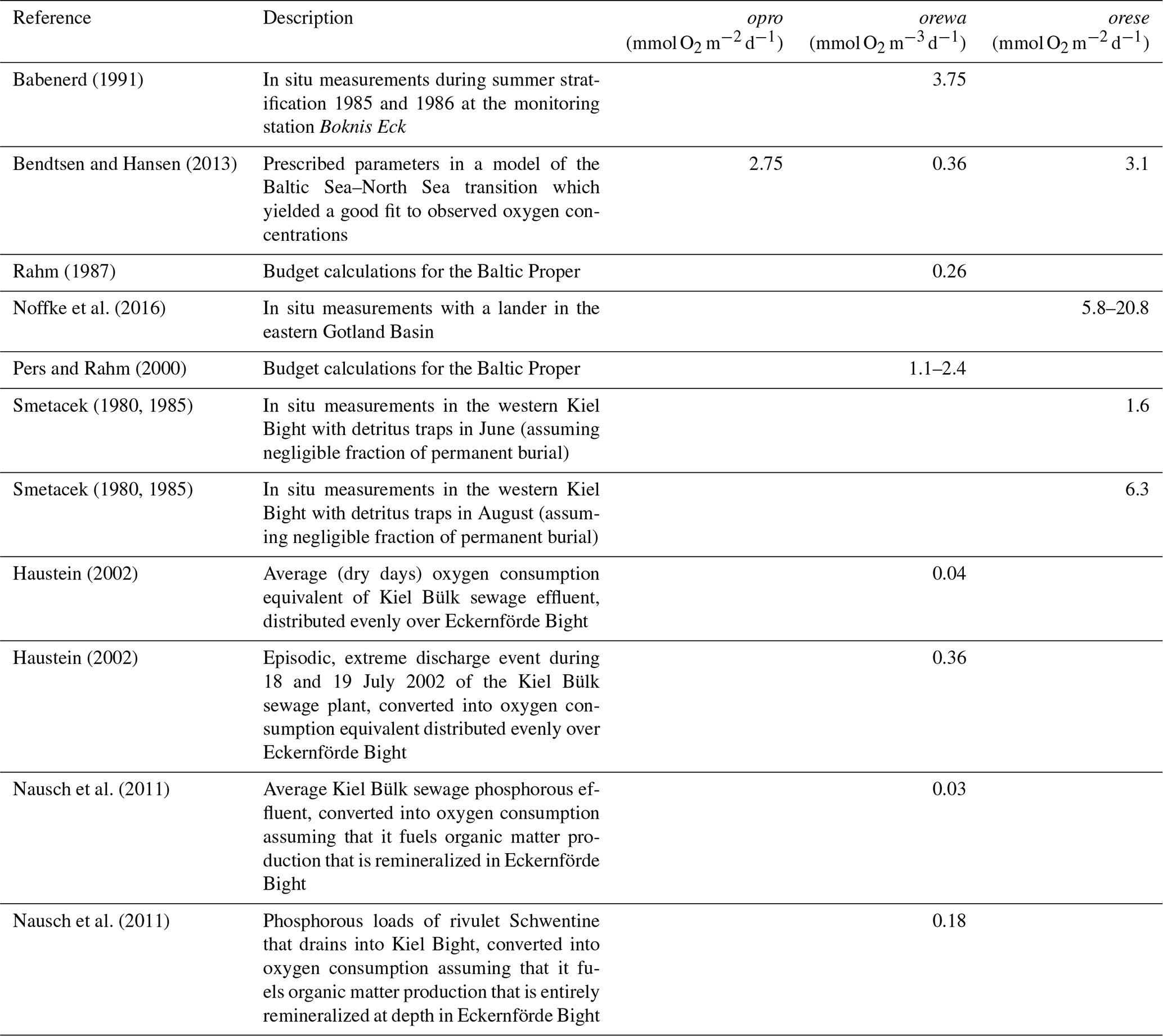
where A und D denote the divergence of the 3-D advective and diffusive fluxes as calculated by the GCM. S denotes biogeochemical oxygen sources and sinks given by the model parameters opro at the sunlit sea surface, by orewa at depth below the compensation depth zco, and by orese in the lowermost wet model grid box. These parameters determine how much oxygen is generated by primary production (opro) and how much is consumed at depth (orewa) and in the sediment (orese). The respective parameter choices are based on literature values listed in Table 1. Following Babenerd (1991) and based on Ærtebjerg et al. (1981) we assume that the subsurface oxygen consumption rates are rather uniform throughout KB, EB, and up into the Danish straits. This assumption is necessitated by our lack of direct measurements of consumption rates in EB. EckO2 prescribes climatological monthly mean consumption rates.
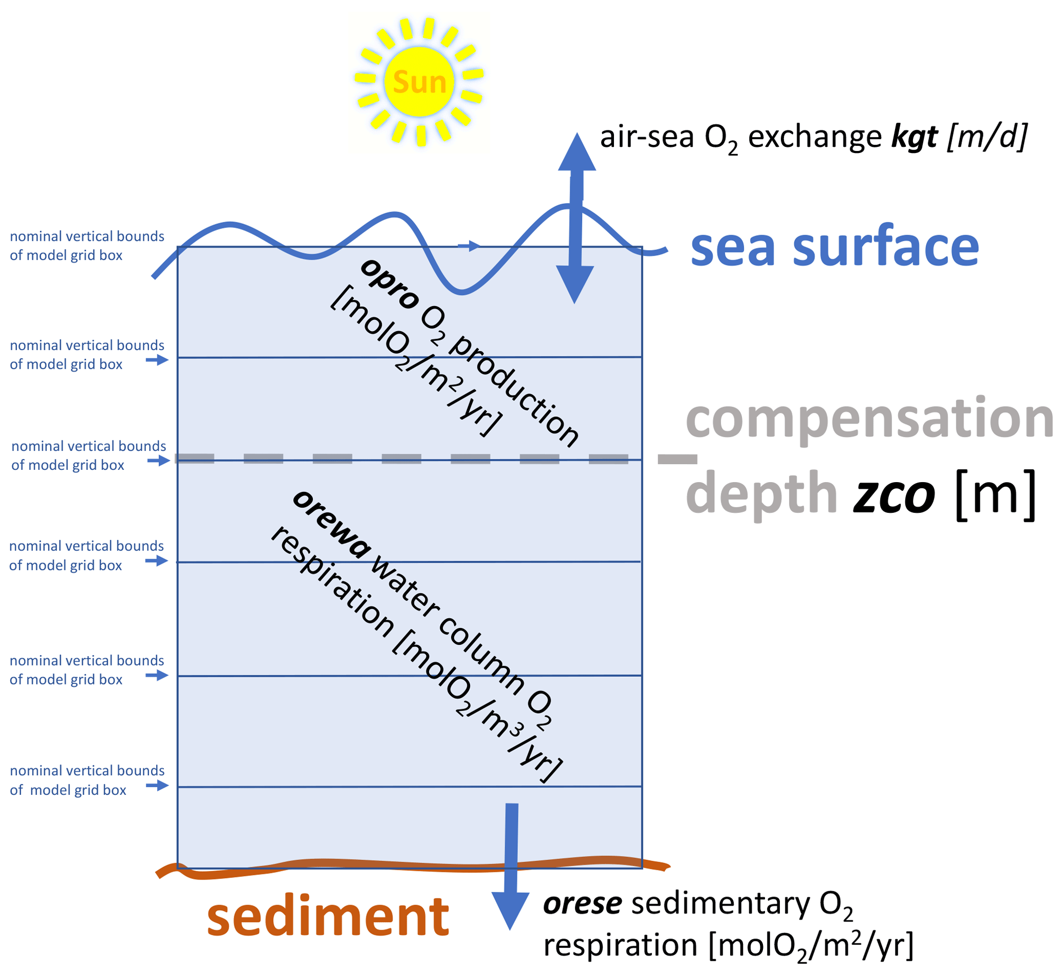
Figure 3Schematic of dissolved oxygen module EckO2. EckO2 calculates sinks and sources of oxygen throughout the water column for every grid box. These terms are then passed to the 3-D general ocean circulation that handles the effect of advection and diffusion. The velocity of the air–sea gas exchange is determined by the piston velocity kgt. Above the compensation depth zco, primary production produces oxygen at a rate prescribed by the model parameter opro. Below the compensation depth zco, respiration of organic matter consumes dissolved oxygen at a rate prescribed by orewa. At the bottom, prescribed oxygen fluxes orese mimic the oxygen consumption of the sediment that is fueled by the transfer across the water–sediment boundary. Table 2 summarizes respective parameter settings.
Table 1Estimates of oxygen consumption and production converted to respective model parameters of the EckO2 module. Conversions may include division by the average water depth and area of Eckernförde Bight (see Sect. 2.1.1), a O2:C ratio of 1.1, and a C:P ratio of 106.
Note that our choice of oxygen consumption rates (Table 2) corresponds to a best guess at the higher end of published estimates (Table 1). To this end the simulations including these local sources and sinks of oxygen provide an upper bound on the effects of local biotic processes on local oxygen dynamics in EB. A lower bound is explored by setting local consumption and production to zero.
2.2 Observations
We use data from the regular monitoring program of the Landesamt für Landwirtschaft, Umwelt und ländliche Räume (LLUR). Respective approximate monthly observations of salinity, temperature, and oxygen covered the entire hindcast period at the monitoring station Buoy 2a (location marked in Fig. 2). Typical surface concentrations of dissolved oxygen are around a few hundred millimoles O2 per cubic meter (mmol O2 m−3), predominantly set by physical solubility as a function of temperature and salinity (and rather constant atmospheric concentrations). At depth, however, oxygen sinks can accumulate oxygen deficits until critical thresholds for the survival of animal or even plants are undercut. Common denominations for critical thresholds are hypoxic, suboxic, and anoxic conditions. Their respective values are, however, fuzzy. Here, we follow Gray et al. (2002) and define the threshold values for hypoxia as a concentration of dissolved oxygen of 2 mg O2 L−1, which corresponds to ≈60 mmol O2 m−3. The relevance of this threshold is that it limits the survival of most fish (Hofmann et al., 2011). In addition we consider a second threshold of 4 mg O2 L−1 corresponding to ≈120 mmol O2 m−3. This value is used as an indicator for the eutrophication of stratified water bodies (such as EB) by the Baltic Marine Environment Protection Commission (Helsinki Commission – HELCOM, 16th Meeting of the Intersessional Network on Eutrophication Helsinki, Finland, 29–30 January 2020), and as such it is of relevance to the stakeholder LLUR.
Among the challenges in simulating oxygen dynamics is that both biotic parameters (determining oxygen respiration; Sect. 2.1.6) and the antagonistic abiotic parameters (that control ventilation with surface water high in oxygen such as, for example, vertical diffusivity; Sect. 2.1.2) are uncertain. Our approach is to run an ensemble of simulations encompassing a plausible range of settings. These settings are listed in Table 2. We compare low, medium, and high levels of diffusivity (tagged LoMix, MedMix, and HighMix, respectively) and, further, simulations which totally neglect local sources and sinks of oxygen (tagged Rem for “remote biotic effects only”) versus those featuring a best guess of local sources and sinks that are on the higher end of published estimates (cf. Table 1 with Table 2). This section identifies the most realistic simulations which will be considered in the following. The ultimate goal is to chose parameter settings which cover the contemporary uncertainty range.
Table 2List of model parameter settings for the EckO2 module and diffusive background mixing in MOMBE: κv refers to vertical background mixing (diffusivity), and opro, orewa, and orese refer to monthly (one value per month starting with the January value) oxygen production, water column oxygen respiration, and oxygen consumption by the sediment, respectively (cf. Fig. 3). Values for orewa and orese are derived from the published estimates listed in Table 1; opro is calculated as residual assuming instant equilibration of sedimentary fluxes.
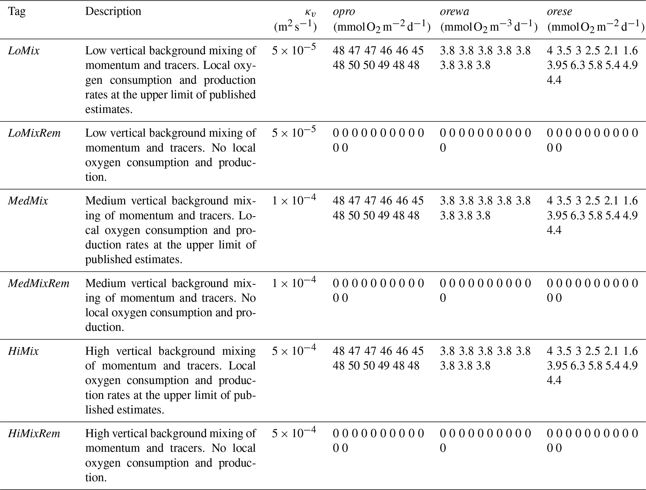
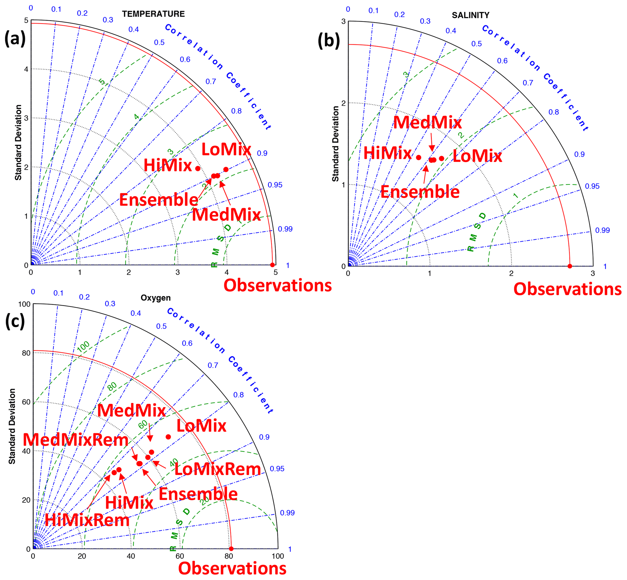
Figure 4Model assessment (Taylor plots) at station Buoy 2a in the interior of EB (Fig. 2). Observational data and model output refer to the 2000 to 2015 period. The simulation tags are defined in Table 2: LoMix, MedMix, and HiMix denote the levels of diffusive background mixing. Rem indicates remote effects of biogeochemical sources and sinks of oxygen only (i.e., no local oxygen consumption in EB.
Figure 4 shows Taylor diagrams which compare simulated and observed temperature, salinity, and oxygen. The simulations with high diffusivity (HiMix and HiMixRem) feature the lowest performance in reproducing the observed variability in temperature, salinity, and oxygen. This is consistent with an assessment of simulated velocities by Marlow (2020). We thus discard these simulations from the analysis. The more realistic simulations LoMix and HiMix are very similar irrespective of whether we account for local sources and sinks of oxygen or not. We conclude (from Fig. 4) that the lower values for the diffusivity are more realistic and that local sources and sinks of oxygen are apparently of minor importance within EB.
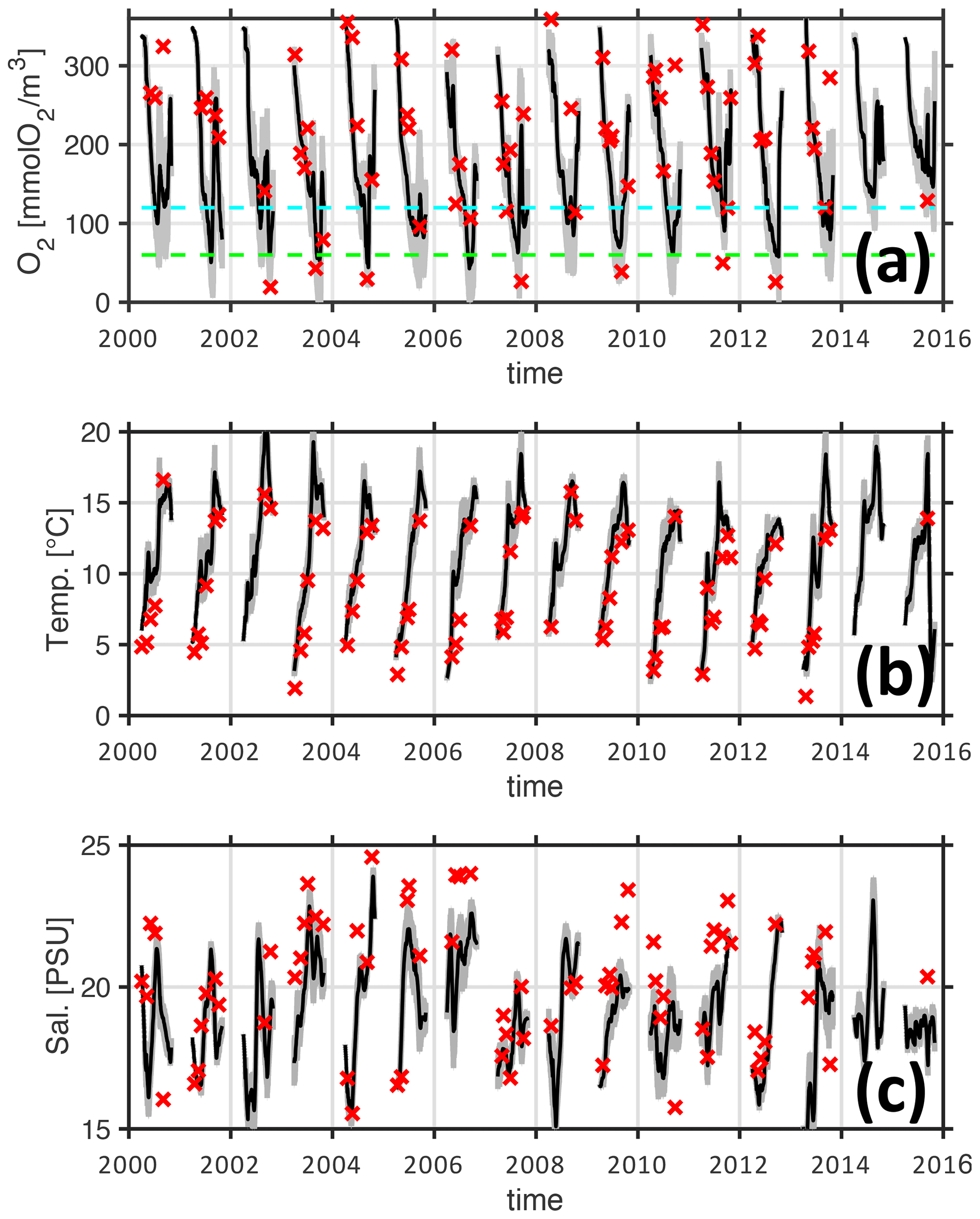
Figure 5Simulated and observed oxygen concentrations at the bottom (20 m depth) of the monitoring station Buoy 2a. Panels (a–c) refer to oxygen concentrations, temperature, and salinity, respectively. Red crosses denote observations. The black line denotes the ensemble mean of the simulations MedMix and LoMix. The gray line envelopes the ensembles' extremes at any given time. The horizontal dashed cyan and green lines in panel (a) show 120 and 60 mmol O2 m−3 hypoxia thresholds, respectively.
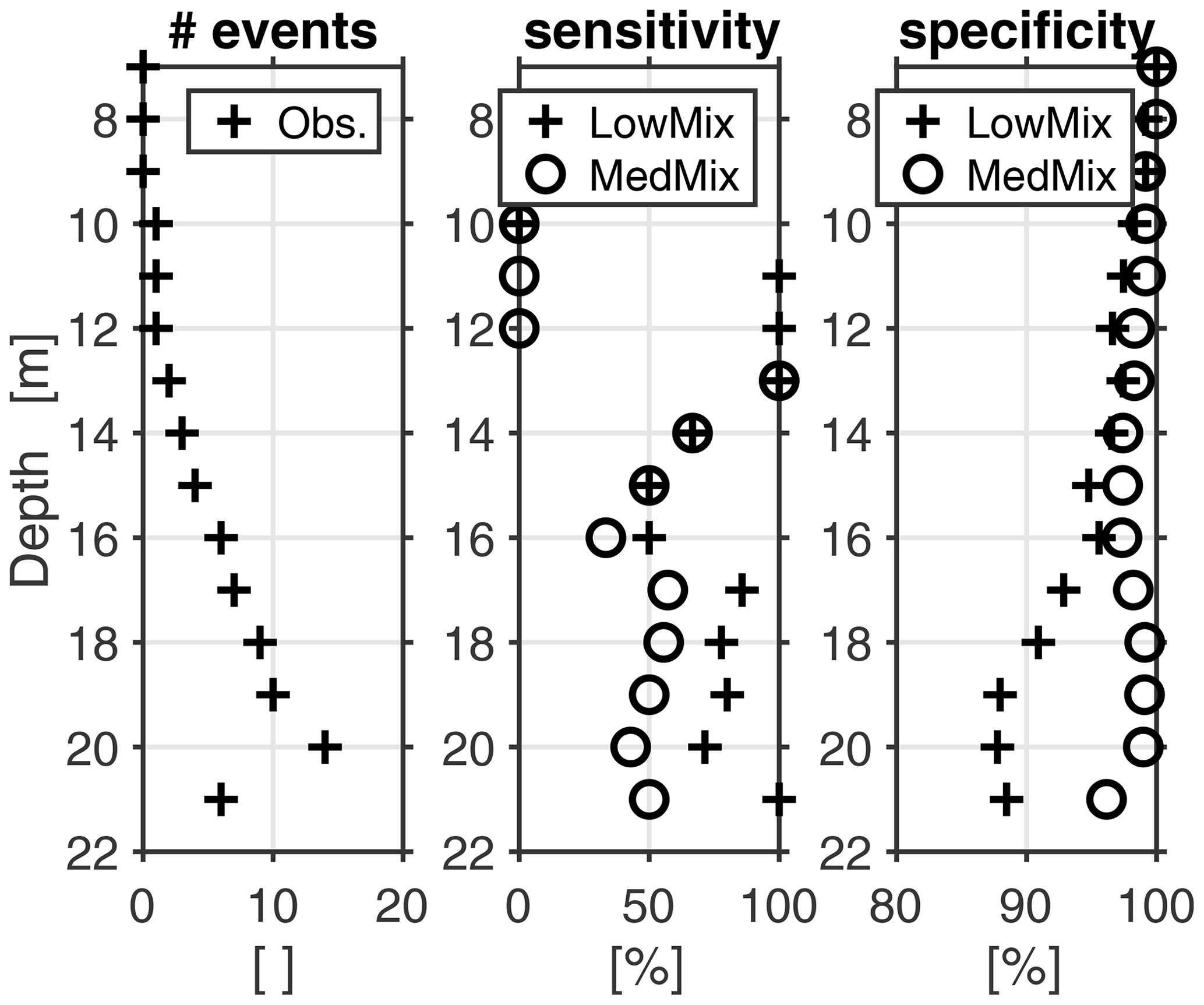
Figure 6Fidelity of hindcasted hypoxic events (oxygen threshold of 120 mmol O2 m−3) at station Buoy 2a.
Figure 5 shows simulated and observed oxygen concentrations at the bottom of the monitoring station Buoy 2a for the years 2000–2015. The respective months of April to October are shown. November to March are omitted because these months feature high concentrations of dissolved concentrations beyond our scope of interest. The overall impression is that the model retraces the dynamics of temperature, salinity, and oxygen reasonably well. Figure 6 provides a more quantitative estimate of the fidelity in reproducing hypoxic events (as defined by the 120 mmol O2 m−3 introduced in Sect. 1) at the monitoring station Buoy 2a. It shows sensitivity and specificity achieved with the simulations LoMix and MedMix that account for local sources and sinks of oxygen: LoMix typically simulates ≈70 % true positives and ≈10 % false positives. MedMix, in comparison, simulates only several percent false positives but fails to identify every third event (i.e., ≈70 % true positives).
We start with exploring the simulated residence and ventilation timescales (Sect. 4.1) for the simulations LoMix and MedMix. This provides a base for understanding the dynamics behind our hindcast presented in Sect. 4.2. A complementary case study of the intense hypoxic event 2017 is presented in Sect. 4.3. Section 4.4 describes the application of artificial intelligence for feature selection and extraction of the predictive capability of monitoring data at station Boknis Eck at the entrance of EB to forecast hypoxia within EB at the monitoring station Buoy 2a.
4.1 Residence and ventilation times
The estimates of residence and ventilation times are calculated with “artificial clocks”, as described in Sect. 2.1.5. Both model versions LoMix and MedMix show similar results: the water with the longest residence time is found at the end of EB in the interior close to the city of Eckernförde (Fig. 7). Typical values are of the order of 1 month for both exemplary months, August and October. Overall, MedMix shows lower values than LoMix indicating that vertical diffusive processes promote the horizontal exchange of water between EB and KB. This makes sense because the longest residence times can be found at the surface (Fig. 8), suggesting that, on average, water enters the bight at depth and leaves the bight at the surface. A stronger vertical diffusivity is then associated with an accelerated rate of surface water renewal by deep water with shorter residence times.
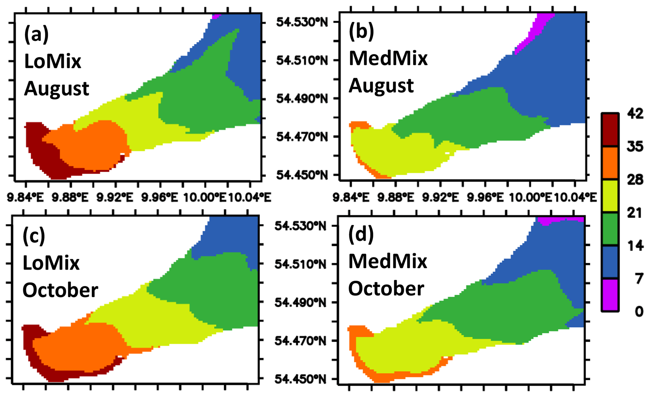
Figure 7Simulated climatological estimate of the residence time of water parcels in EB. The units are days elapsed since the water flushed into the bight. The estimate refers to the longest residence time found in local water columns. Panels (a) and (b) refer to August calculated by the simulations LoMix and MedMix, respectively. Panels (c) and (d) refer to October calculated by the simulations LoMix and MedMix, respectively. Note that the model domain extends beyond the eastern boundary shown here (see also Fig. 2).
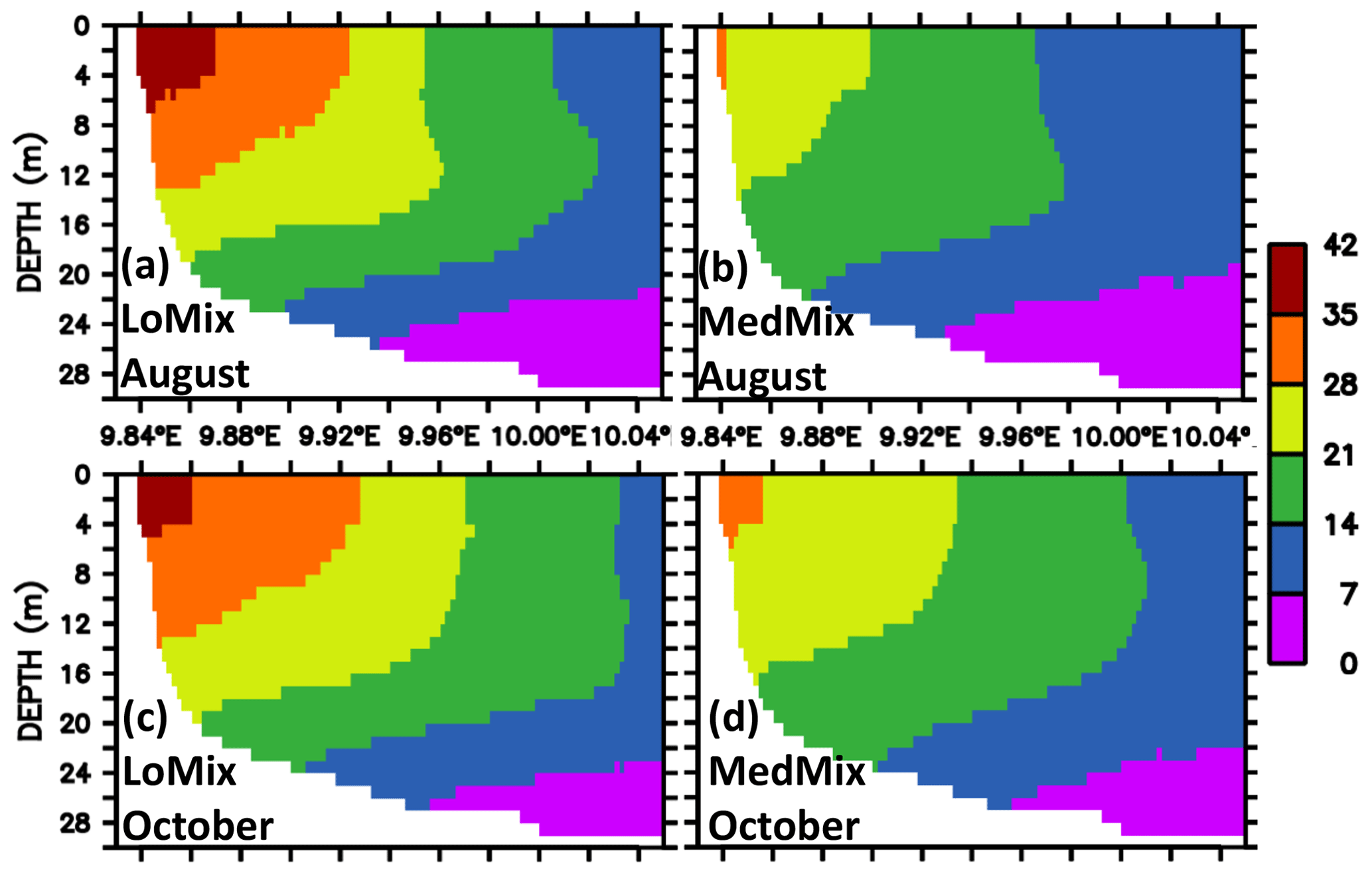
Figure 8Simulated climatological estimate of the residence times of water parcels in EB. The units are days elapsed since the water flushed into the bight. Sections along EB are shown. Panels (a) and (b) refer to August calculated by the simulations LoMix and MedMix, respectively. Panels (c) and (d) refer to October calculated by the simulations LoMix and MedMix, respectively. Note that the model domain extends beyond the eastern boundary shown here (see also Fig. 2).
The distribution of ventilation times or age is similar to that of residence times in that the highest values are generally found within the bight towards Eckernförde (Fig. 9). The horizontal gradient is more pronounced in the simulation with lower mixing, while higher prescribed vertical background mixing equalizes the effective ventilation processes horizontally. In terms of vertical distribution, age has, in contrast to the residence time, high values at depth and low at the surface, where it is reset to zero (Fig. 10).
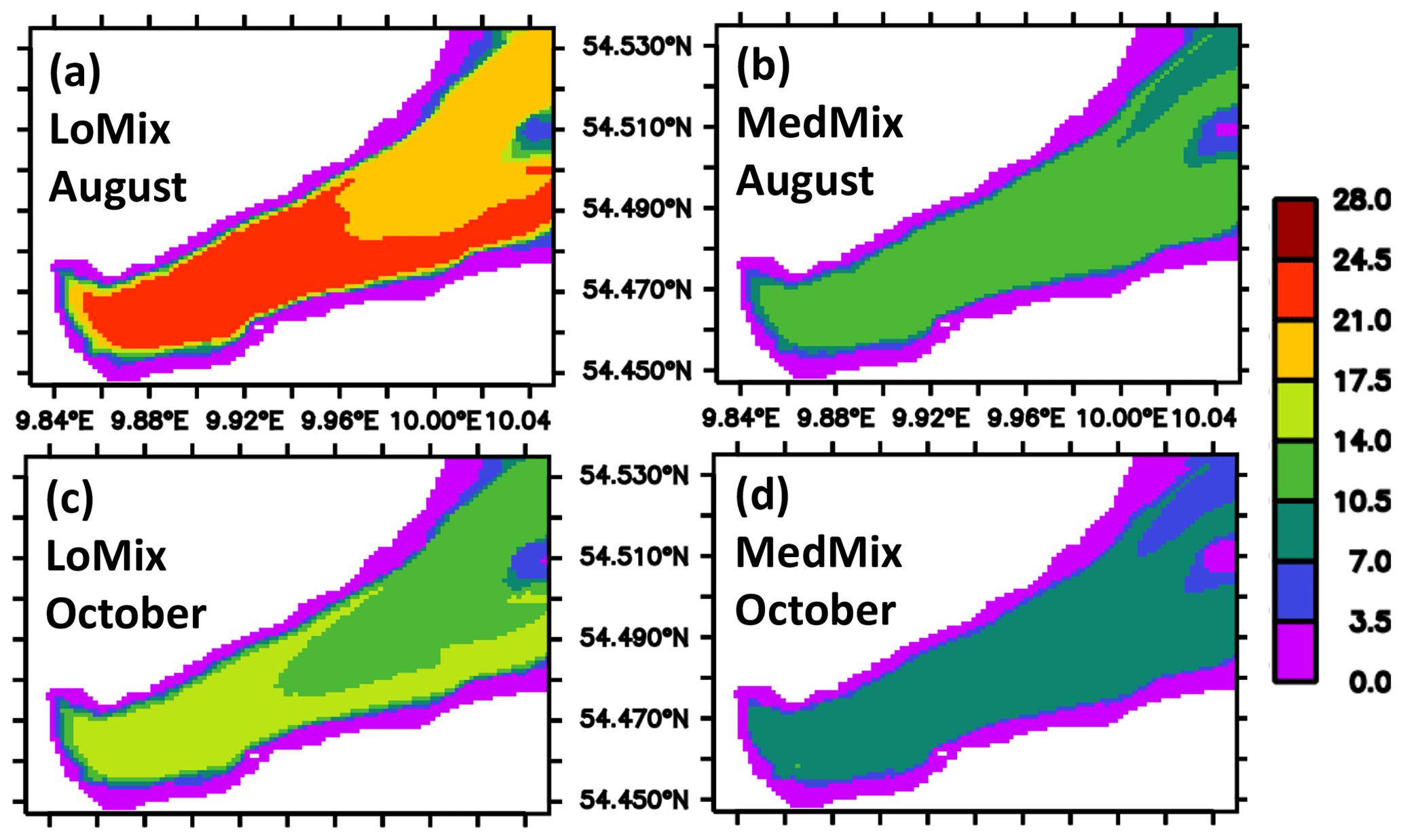
Figure 9Simulated climatological estimate of local ventilation. The color shading denotes the time elapsed (age) since bottom water has been in contact with the atmosphere in units of days. Panels (a) and (b) refer to August calculated by the simulations LoMix and MedMix, respectively. Panels (c) and (d) refer to October calculated by the simulations LoMix and MedMix, respectively. Note that the model domain extends beyond the eastern boundary shown here (see also Fig. 2).

Figure 10Simulated climatological estimate of local ventilation. The color shading denotes the time elapsed (age) since water parcels have been in contact with the atmosphere in units of days. Sections along EB are shown. Panels (a) and (b) refer to August calculated by the simulations LoMix and MedMix, respectively. Panels (c) and (d) refer to October calculated by the simulations LoMix and MedMix, respectively. Note that the model domain extends beyond the eastern boundary shown here (see also Fig. 2).
In summary, we find that residence times and age are of similar magnitude. This suggests that the first order control of processes that determine oxygen concentrations in EB is an antagonistic interplay of inflowing water (generally low in oxygen) and the local aeration by vertical exchange with oxygenated surface waters. Biogeochemical processes in the interior of EB are apparently of minor importance for the oxygen dynamics within EB.
4.2 The typical seasonal cycle inside EB
Figure 5 shows a comparison between the observed and simulated temporal evolution of dissolved oxygen concentrations at the bottom of the monitoring station Buoy 2. Most prominent is a pronounced seasonal cycle. The generic explanation for such seasonal cycles in such latitudes is that temperatures and biomass production in the surface waters ramp up in spring, being driven by enhanced levels of photosynthetically available radiation (note, however, that there is an ongoing discussion on this issue: Behrenfeld, 2010; Arteaga et al., 2020; Smetacek, 1985). The biomass eventually sinks to depth where it degrades and issues oxygen consumption. Later in the season, the water column stratifies, and the surface layer heats up, effectively creating a barrier to the exchange of bottom water (deprived of oxygen) and the oxygenated surface waters. As autumn approaches, the surface ocean cools again and weakens the stratified barrier to vertical mixing. This facilitates the wind-driven mixing events that come along with more unstable autumn weather. In winter, convective mixing homogenizes the entire (rather shallow) water column vertically (e.g., Fennel and Testa, 2019; Petenati, 2017). Apparently the model captures this dynamic well; i.e., the ensemble mean of LoMix and MedMix features a high visual correspondence between the respective curves in Fig. 5 (see Fig. 4 for more quantitative estimate).
Based on the hindcast simulation from 2000 to 2015 hypoxic events at station Buoy 2a are most common in August and October with a local minimum of occurrences in September (Fig. 11). This is inconsistent with the generic explanation outlined above, where a period of ever decreasing levels of dissolved oxygen ends in autumn when increasing winds and a pronounced air–sea heat transfer promotes net ventilation. So why do hypoxic conditions deep in EB at station Buoy 2a become more frequent after the September setback despite increasing winds and decreasing thermal stratification? The histograms of bottom oxygen concentrations observed at station Boknis Eck, situated at the entrance to EB (and used to prescribe the conditions of water flowing into EB in the model), suggest that particularly low oxygen concentrations are more frequent in October than in August (Fig. 12). Hence, water entering EB from KB in October is more likely to “import” hypoxia. Note that these considerations are in line with simulations LoMixRem/LoMix and MedMixRem/MedMix, each pair showing in Fig. 4 very little effect of local oxygen consumption within EB, even though (1) the respective biotic local oxygen consumptions are chosen to represent the upper limit of published estimates and (2) the water exchange with KB is hampered by a rigid wall boundary condition.

Figure 11Simulated climatological (2000–2015) occurrence of hypoxia at the monitoring station Buoy 2a. Occurrence refers to the sum of suboxic (i.e., <120 mmol O2 m−3) model grid boxes, identified in climatological daily model output. From November to June suboxic conditions were absent.
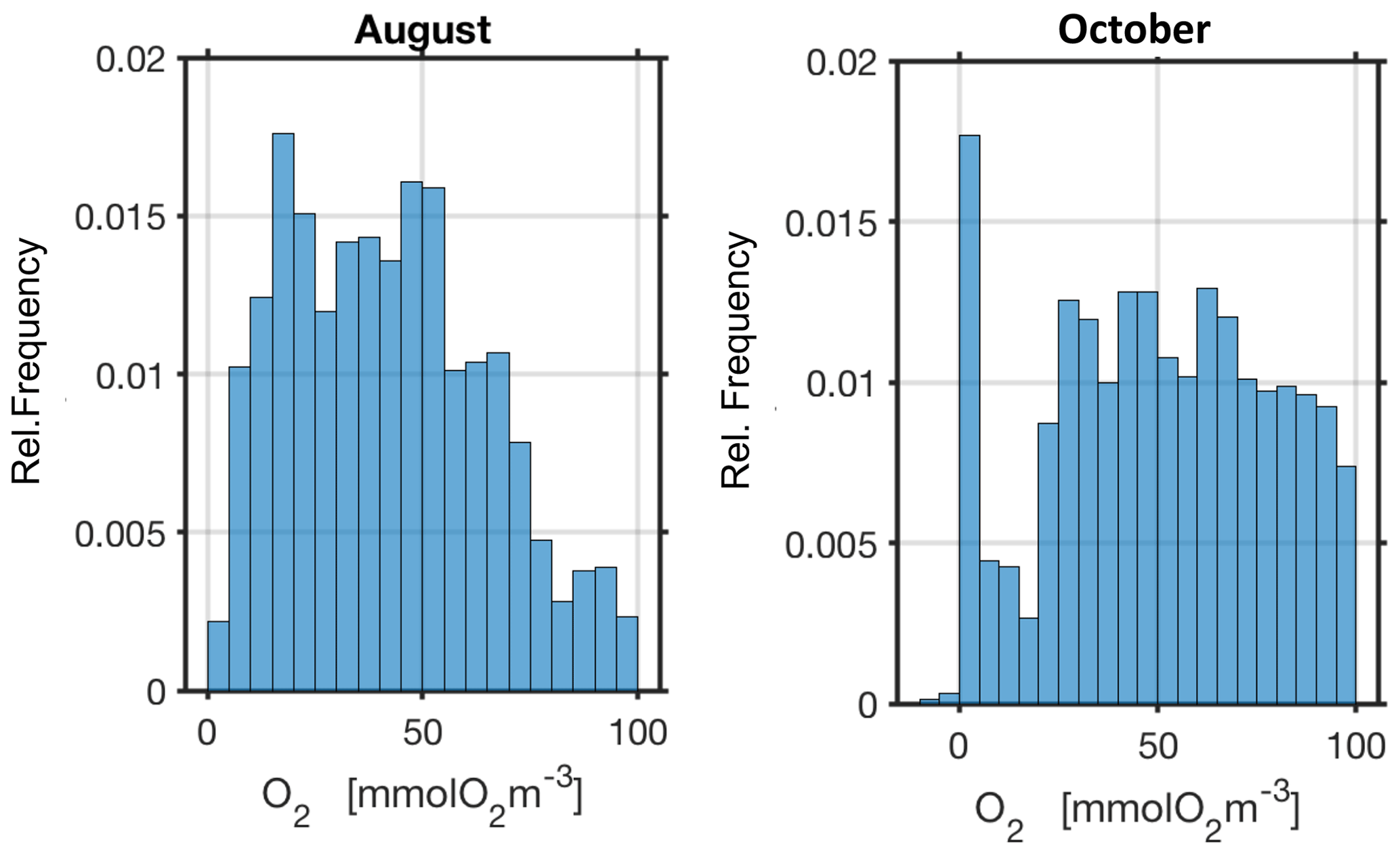
Figure 12Histogram of observed climatological bottom oxygen concentrations at Boknis Eck (capped at 100 mmol O2 m−3).
We conclude that the typical oxygen deficit in late summer is imported along with water from the KB, rather than being produced locally in EB. The following Sect. 4.3 will elucidate the underlying succession of events by means of a detailed case study.
4.3 Hypoxic event 2017
In fall 2017 a particularly pronounced hypoxic event occurred and led to a mass fish-kill incidence. In the following, we analyze this event in the MOMBE LoMix simulation.
Figure 13 shows a sequence of snapshots of simulated hypoxia in EB, starting 20 August and ending at peak conditions on 10 September. Over the course of these several weeks, EB loses oxygen, and hypoxic waters apparently enter the bight at the bottom from the east and move upwards. The notion of “imported” hypoxic conditions is backed by the Hovmöller diagrams of simulated age and residence times at the monitoring station Buoy 2a in Fig. 14: during the buildup of the hypoxic event in EB, the residence time features a local minimum deep inside EB. This suggests the prevalence of water masses “recently imported” from KB (Fig. 14b). Simultaneously, the age features a maximum (Fig. 14a), indicating that the recently imported hypoxic waters are well shielded from ventilation by oxygenated surface waters. Further evidence is provided in Fig. 15, showing that the oxygen decline in EB is contemporaneous with winds blowing out of the bight. These winds drive an overturning circulation, shown in Fig. 16, with surface waters being pushed out of the bight and bottom waters, for continuity reasons, being sucked into the bight at depth. Consequently, we find in Fig. 15 that the oxygen decline at the entrance of the bight (at station Boknis Eck) occurs earlier than the oxygen decline inside the bight (at station Buoy 2a) – just as expected in a system where water enters the bight at the bottom.
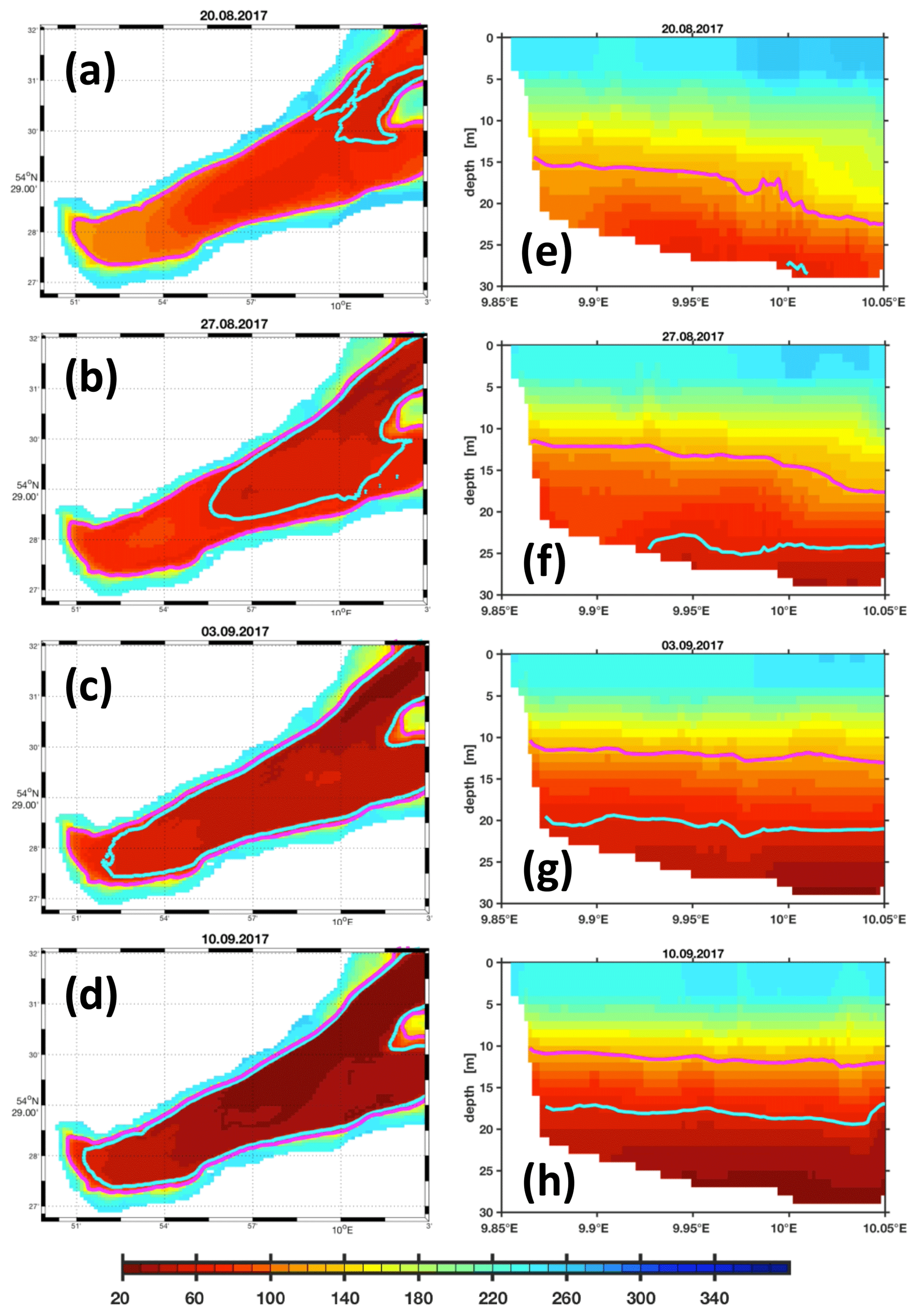
Figure 13Simulation (LoMix) of the 2017 hypoxic event. The colors refer to oxygen concentrations (in mmol O2 m−3). The contours in cyan and magenta show the 60 and 120 mmol O2 m−3 isolines. The left column (a–d) shows oxygen concentrations on the sea floor. The right column (e–h) shows a section through the bight with the city of Eckernförde to the left and the entrance to the bight to the right. (Corresponding animations featuring daily resolution named LoMix_O2_Bottom_2015.m4v and LoMix_O2_zonal_2017.m4v are archived at https://doi.org/10.5281/zenodo.4271940.) Note that the model domain extends beyond the eastern boundary shown here (see also Fig. 2).
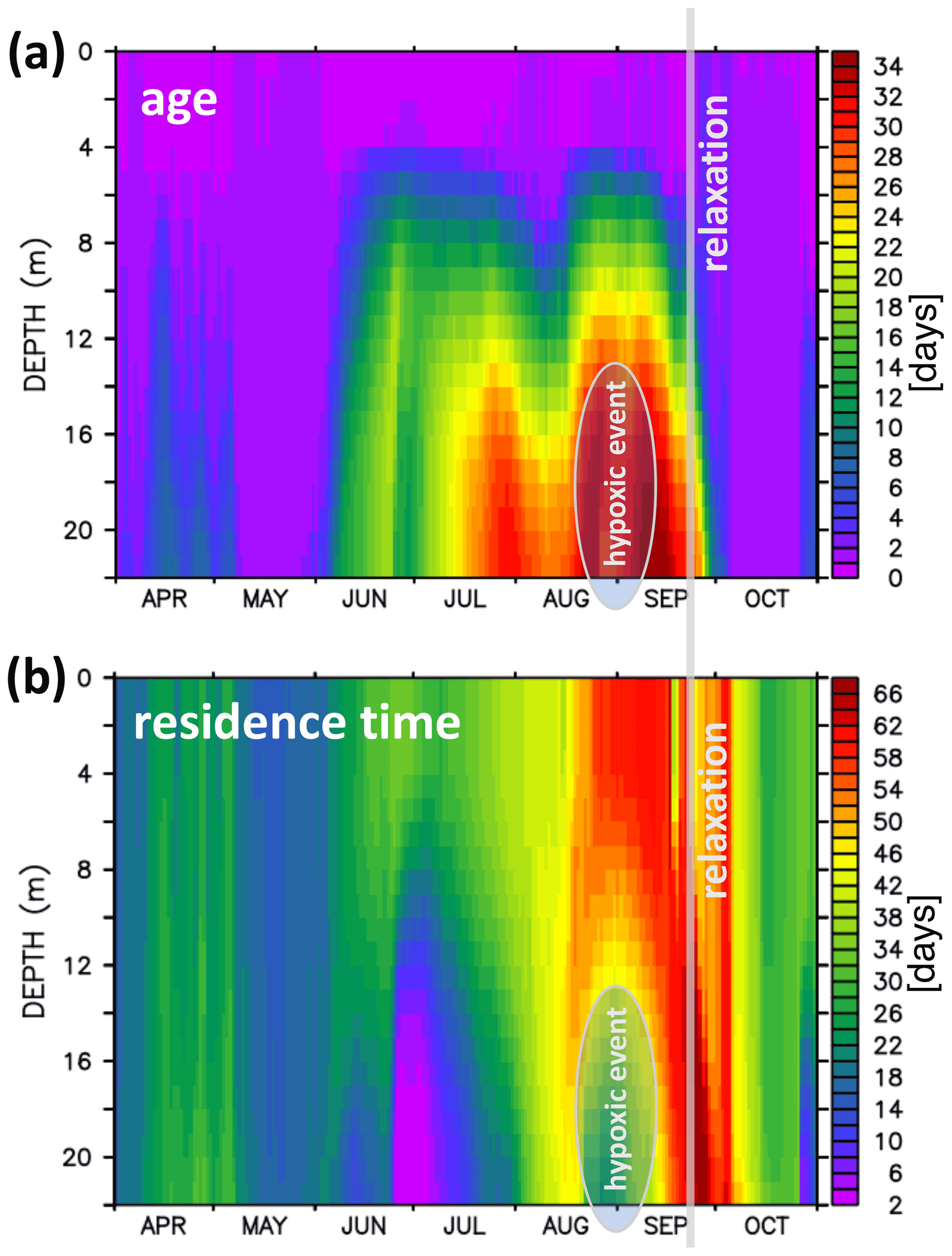
Figure 14Hovmöller diagrams of simulated water age and residence time at the monitoring station Buoy 2a (a and b, respectively). The oval marking in August–September highlights the 2017 hypoxic event. The vertical gray line marks the start of the relaxation phase ending the hypoxic event.
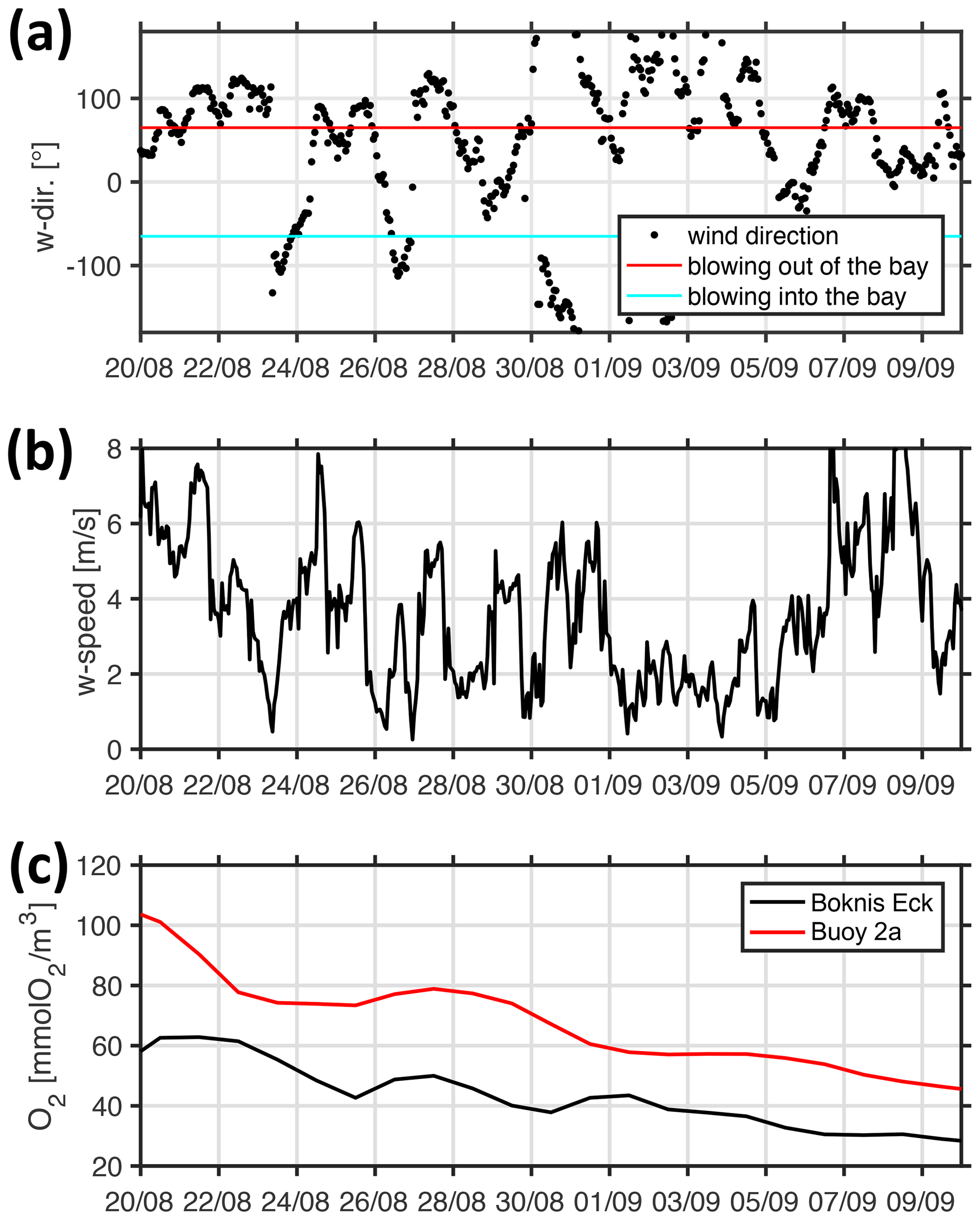
Figure 15Simulated temporal evolution of (a) wind direction, (b) wind speed, and (c) bottom oxygen concentrations during the buildup of the 2017 hypoxic event. The black and red lines in panel (c) refer to station Boknis Eck at the entrance and station Buoy 2a deep inside EB, respectively.

Figure 16Simulated, daily mean zonal currents during the buildup of the 2017 hypoxic event shown in Figs. 13–15. Green to blue colors characterize flows to the east (towards the KB). Yellow to red colors indicate flows to the west (into EB). The unit is kilometers per day (km d−1). The depicted section has an extension of ≈13 km. Note that the model domain extends beyond the eastern boundary shown here (see also Fig. 2).

Figure 17Simulated temporal evolution of (a) wind direction, (b) wind speed, and (c) bottom oxygen concentrations during the relaxation phase that terminates the 2017 hypoxic event. The black and red lines in panel (c) refer to station Boknis Eck at the entrance and station Buoy 2a deep inside EB, respectively.
During the relaxation phase that terminates the 2017 hypoxic event, the processes are reversed: Fig. 17 shows that the winds are blowing consistently into the bight for more than a week. Consequently, water is pushed into the bight at the surface, having nowhere to go. Some of the well-oxygenated surface water is subducted to depth and subsequently leaves EB at depth. Just as expected, the increase in oxygen at the monitoring station Buoy 2a inside the bight occurs earlier than the corresponding oxygen increase at the entrance station Boknis Eck. The oxygen levels at Boknis Eck now lag behind Buoy 2a by approximately 1 week.
In summary, we identified a governing mechanism by which EB is – depending on wind direction – either (1) impacted by imported low-oxygenated waters from KB or (2) being flushed by oxygenated surface water that is subducted to depth in the interior of EB and is exported at depth to KB – whereby EB is effectively ventilating KB.
Open questions, however, remain. Of particular interest is the questions of why some years are hit especially hard by hypoxia and whether such events are predictable days or weeks in advance. Such predictions may, for example, allow for netting and landing of doomed fish. The following section applies artificial intelligence (AI) to pursue these questions.
4.4 AI-based feature selection and time series prediction
The following section explores the statistical relations between the simulated time series at station Buoy 2a deep in the bight and Boknis Eck at the entrance of the bight. The major aims are (1) to gain further mechanistic insight and (2) to develop a surrogate model for the stakeholder that may be implemented on off-the-shelf desktop computers, smart phones, or even on very low cost (<10 EUR) embedded devices rather than necessitating access to a super-computing facility (as is the case with the full-fledged coupled model). This section is motivated by recent and encouraging success in emulating general circulation models (e.g., Castruccio et al., 2014), ecosystem models (e.g., Fer et al., 2018), the tremendous success in machine learning and data-driven methods in fluid dynamics (as summarized, for example, by Brunton et al., 2020a), and the sneaking suspicion that “…the most pressing scientific and engineering problems of the modern era are not amenable to empirical models or deviations of first principles…” (Brunton et al., 2020b).
In the following, we describe the application of shallow and deep feed-forward artificial neural networks (ANNs) to forecast bottom oxygen concentrations deep inside EB at the Buoy 2a monitoring station 2 weeks in advance from the atmospheric conditions and the regularly sampled monitoring station Boknis Eck at the entrance of the bight. The forecast range is chosen as a compromise between the time needed for mitigation measures (e.g., by netting and landing of doomed fish) and forecast accuracy which typically degrades with forecasting range. During the course of this exercise we will use different combinations of predictors (or input data) and test their impact on the forecast skill – a process also referred to as capacity estimation and feature selection (e.g., Sbalzarini et al., 2002). Note, however, that a comprehensive analysis of time series forecasting, which must include traditional statistical approaches in addition to machine learning methods (Makridakis et al., 2018), is beyond the scope of this article.
4.4.1 Capacity estimation and feature selection
For training the ANNs, we draw our training (80 %) and validation data (20 %) randomly from the 2000 to 2016 model hindcast. We hand-design features (input data) and test their respective capacity to forecast bottom oxygen concentrations at station Buoy 2a (target data). Hand-designed features are “…two edged swords” (e.g., Reichstein et al., 2019): they can be seen as an advantage because they give us control of the explanatory drivers which may be used to promote system understanding. On the other hand, hand-designed features are typically suboptimal. To this end our results here provide a lower bound on the potential of ANNs for the task at hand.
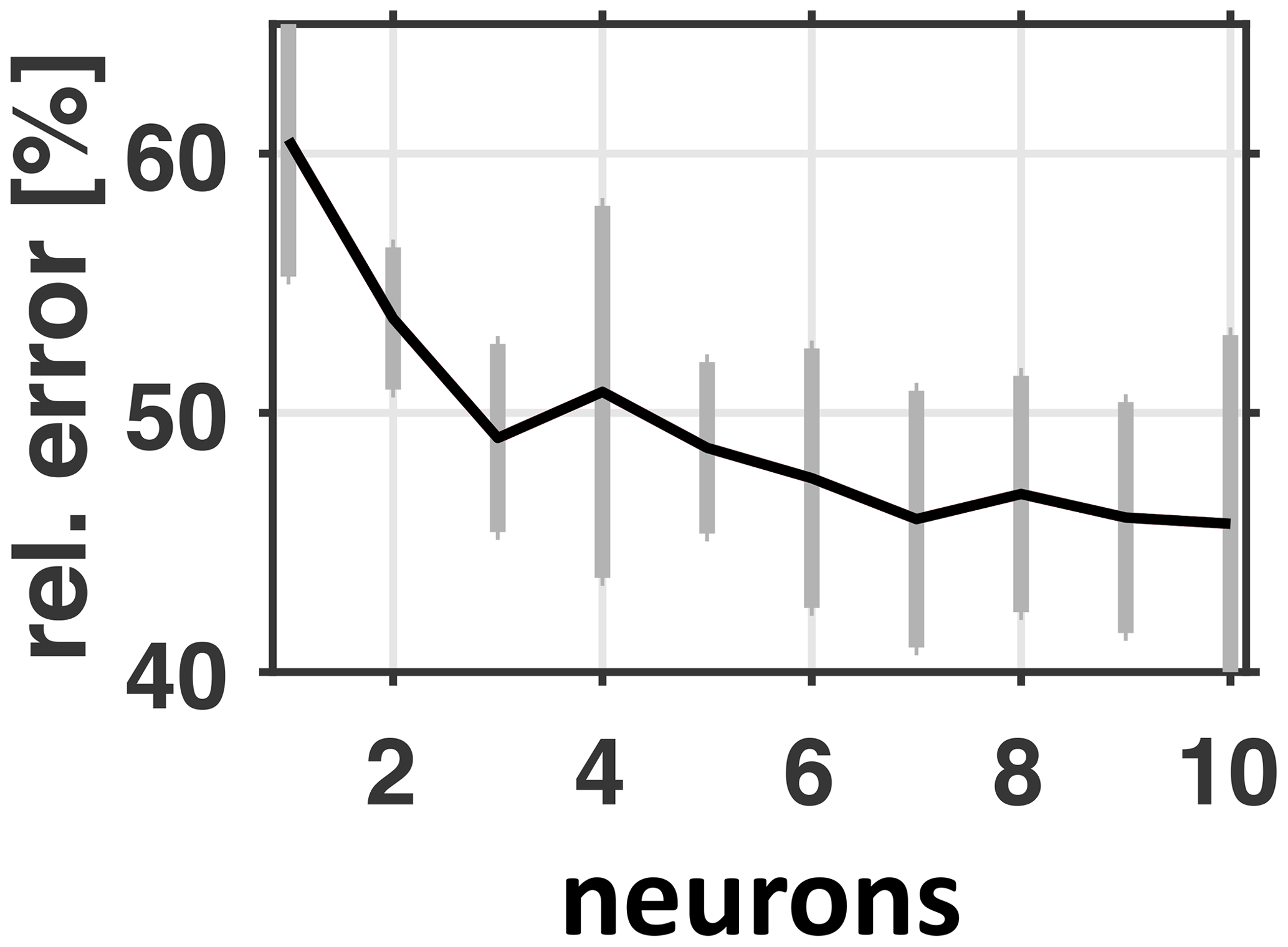
Figure 18ANN error relative to naive persistency forecast versus the number of neurons in the hidden layer. The black line features the best ANN parameter setting found within an ensemble of 30 optimizations for each of the number of neurons tested. The gray bars denote the ensemble's standard deviations.
The ANN is trained using the Levenberg–Marquardt algorithm (Marquardt, 1963) applied to neural network training following Hagan and Menhaj (1994) and Hagan et al. (1996). Each training is repeated 30 times, each of which may yield (slightly) differing results because, depending on the (random) initialization of weights, the algorithm may terminate in potentially differing local optima of the cost function. As cost function we choose mean-squared errors (calculated from MOMBE output and the ANN prediction designed to mimic the MOMBE output). Figure 18 shows respective cost as errors relative to a naive biweekly persistency forecast based on bottom oxygen concentrations at the monitoring station Boknis Eck: apparently the ANN's performance converges at 45 % relative to the persistency forecast. Defining this as the Pareto frontier suggests a Pareto optimal of 56 %, which corresponds to one or two nodes. The idea of opting for a rather parsimonious two-node model that scores 80 % of the Pareto Frontier rather than 100 % is to reduce the risk of overfitting which may hinder generalization. Further, parsimonious models are easier to interpret than their complex counterpart such that their robustness is easier to assess. This is especially important because we have no straightforward way to extract human semantics from the “rules” the neural network learned during the optimization process that related our input features to the target bottom oxygen concentrations at station Buoy 2a.
We start with a shallow (one input, one hidden, and one output layer) ANN utilizing the full vertical profiles of temperature, salinity, and oxygen along with a biweekly wind forecast totaling 106 input features (given by the three 1 m resolution vertical profiles of temperature, salinity, and oxygen down to 26 m depth and the 14 daily forecasts of zonal and meridional winds each). This setup is based on an optimistic estimate of the number of features available to stakeholders. Specifically, we assume to have access to a correct biweekly wind forecast along with one full vertical profile each of temperature, salinity, and oxygen at the monitoring station Boknis Eck located at the entrance of EB (i.e., the 106 features introduced above).
Figure 18 suggests that the Pareto Frontier is at 45 %, corresponding to a 55 % reduction in error relative to the persistence model. A total of 80 % of this yields a Pareto Optimal of 56 %. This corresponds to one or two nodes. Additional tests with deeper ANNs featuring up to 10 hidden layers with two nodes were unsuccessful in that respective errors were always higher than 50 %. We conclude that a simple two node shallow ANN already features a reasonable performance, and two input features, of the 106 tested, may suffice to capture the main effects.
Table 3Capacity estimation of input features. This table relates the fidelity of biweekly walk-forward ANN forecasts of bottom oxygen concentrations at the monitoring station Buoy 2a with data from station Boknis Eck fed to the ANN. The average of wind speed squared refers to respective biweekly forecasts of zonal winds. The error is the RMS deviation between the (computationally cheap) ANN projection and simulated (computationally expensive; full-fledged coupled biogeochemical ocean circulation model) bottom oxygen concentrations at Buoy 2a relative to the respective RMS of the persistence model (which naively assumes that Boknis Eck bottom oxygen concentrations will persist for 14 d at Buoy 2a.
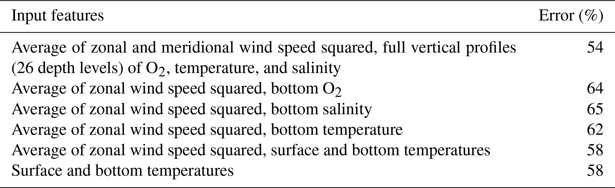
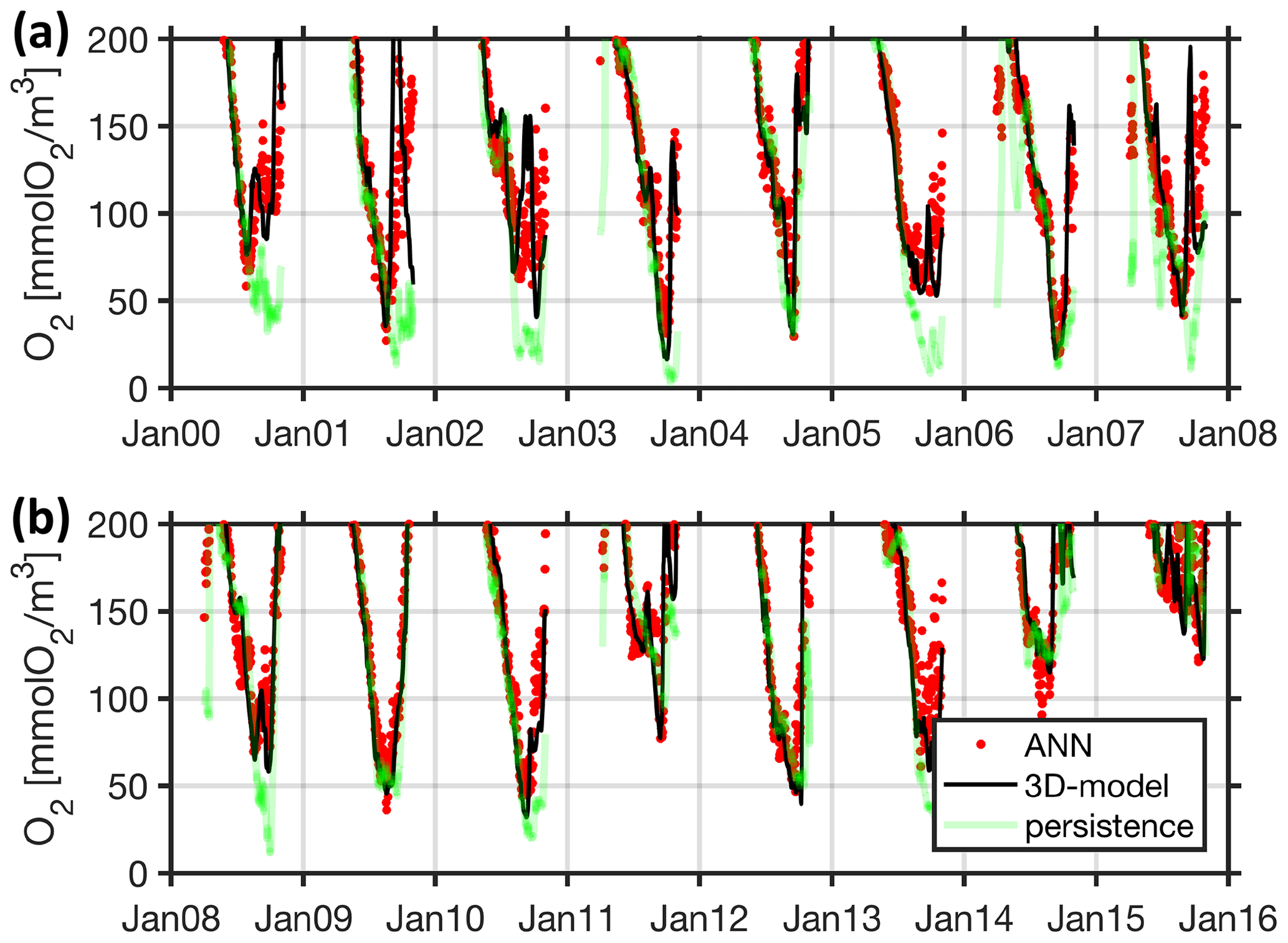
Figure 19Walk-forward performance of ANN based on training and testing data (corresponding to 80 % and 20 % of the data shown here). The black line shows bottom oxygen concentrations at station Buoy 2a as simulated with the full-fledged and computationally expensive 3-D coupled ocean circulation biogeochemical model. Each of the red dots denotes a respective biweekly walk-forward (computationally cheap) ANN forecast utilizing surface and bottom temperatures at station Boknis Eck only. For comparison, the green line features a naive biweekly persistency forecast based on bottom oxygen concentrations at station Boknis Eck.
Table 3 summarizes our effort to identify the most predictive features by backward elimination (e.g., Dietterich, 2002). Using combinations of only 15 features comprised of biweekly zonal wind speed and the bottom values of either temperature, salinity, or oxygen yielded a moderate degradation in performance of only 10 % (Table 3 entries 2 to 4). Pushing further we identified a combination of two features only that are, on the one hand, within this 10 % degradation and, on the other hand, especially easy to measure for stakeholders: surface and bottom temperatures at station Boknis Eck. Contrary to intuition, adding wind forecasts does not improve the ANNs fidelity (compare entries 5 and 6 in Table 3). Even so, the ANN fits the training and validation data remarkably well (Fig. 19). We conclude that the ANN's biweekly forecast exploits links other than those being direct consequences of the wind-driven inflow versus ventilation mechanism identified in Sect. 4.3. Section 4.4.2 puts this exploitation to the test using independent test (model) data.
4.4.2 ANN generalization
This section discusses the fidelity of the two-node ANN using simulated bottom and surface temperatures identified in Sect. 4.4.2 as being parsimonious but – nevertheless – yielding reasonable results compared to more complex architectures, such as deeper nets using more nodes and input data. Here, we use independent test data covering the years 2016 to 2018 of our hindcast simulation. These data have been used neither in training nor during validation so far. To rate the forecast it is compared to the “persistence model”, which assumes that the oxygen concentrations at station Boknis Eck appear 2 weeks later at station Buoy 2a (green line in Fig. 20). The first striking impression of the close-ups in Fig. 20 is that all years feature a similar seasonal decline in bottom oxygen in autumn and this decline generally closely resembles the oxygen decline in Boknis Eck 2 weeks in advance. Large interannual differences, however, occur at the onset of the trend reversal. This “return point” in time is not captured well by the persistency model. These results are consistent with our results in Sect. 4.3 showing that the decline is driven by the import of low-oxygenated waters from KB. Ventilation, however, takes place in the interior of the bight, and its signal reaches station Boknis Eck at the entrance afterwards such that we indeed expect no predictive power of the persistency model under these circumstances. To this end, our ANN clearly outperforms the persistency model in that it predicts an earlier and more realistic recovery of oxygen values during the end of summer/beginning of autumn despite the ANN also exclusively relying on data at the entrance at station Boknis Eck.
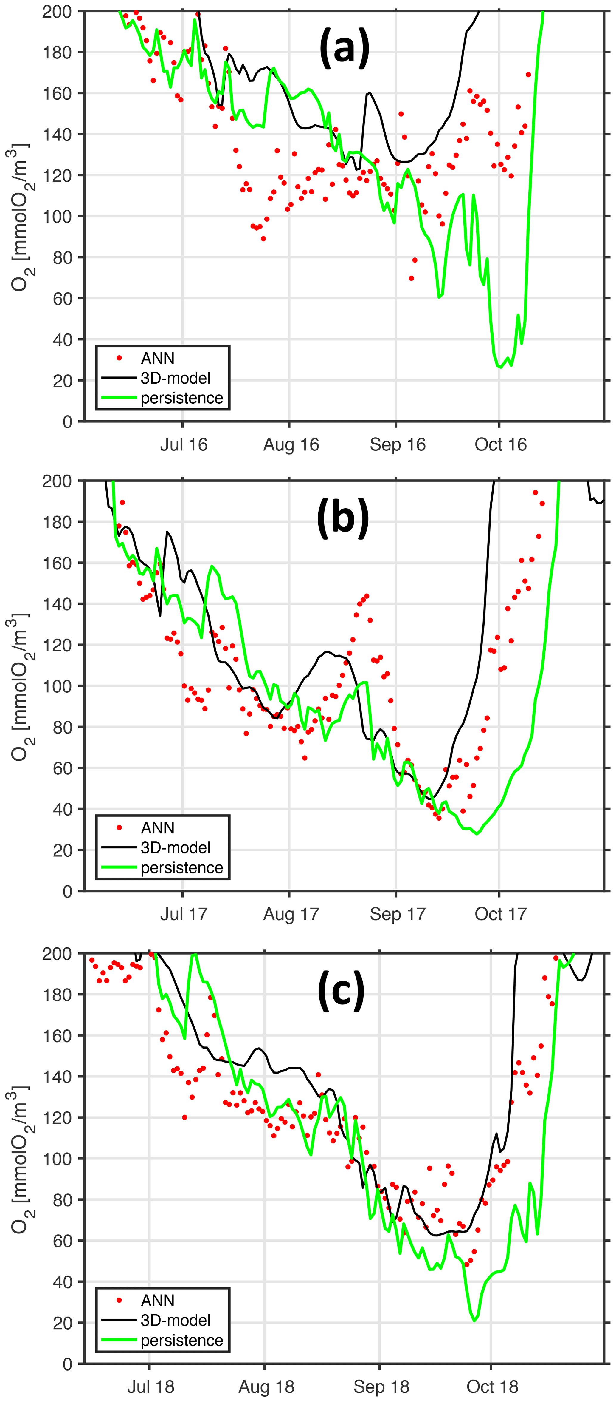
Figure 20Walk-forward validation (generalization) of ANN. Panels (a–c) refer to years 2016, 2017, and 2018. The black line shows bottom oxygen concentrations at the monitoring station Buoy 2a as simulated with the full-fledged and computationally expensive 3-D coupled ocean circulation biogeochemical model. Each of the red dots denotes a respective biweekly walk-forward (computationally cheap) ANN forecast utilizing surface and bottom temperatures at station Boknis Eck only. The green line features a naive biweekly persistency forecast based on bottom oxygen concentrations from station Boknis Eck for comparison.
The ANN essentially and successfully links information regarding season (“derived” from sea surface temperature) and stratification (“derived” from the temperature difference between surface and depth) at the entrance of the bight with oxygen concentration in the interior of the bight – without utilizing information on winds. This clearly emphasizes the role of stratification in putting an end to hypoxic events: EB is in the latitudes of prevailing westerlies, with “prevailing” entailing that the local winds shift back and forth as the weather systems travel east. Any of these wind shifts from westerly to easterly may end an hypoxic event in EB – if the stratification is weak enough (and winds are strong enough) such that oxygenated surface water can be pushed to depth. In a nutshell, if the stratification has sufficiently weakened, you know that the next wind shift will subduct oxygenated water, thereby ending the hypoxic event.
In summary, the ANN features a remarkable performance given that it simply relies on two temperature measurements at the entrance of the bight. This performance is owed to the importance of stratification in setting the length of hypoxic events: eroding stratification preconditions the wind-driven downwelling or subduction of oxygenated surface waters which ends hypoxic events. Given that the EM is positioned in the prevailing westerlies, the winds regularly change to easterlies, but this only drives substantial oxygenation (replacement) of bottom waters if the stratification is weak enough to be penetrated. Hence, there is a high explanatory power of surface and bottom temperatures at the entrance of EB to predict the dynamics of hypoxia deep in EB.
Oxygen concentrations are controlled by the antagonistic interplay of respiration and ventilation processes, both of which may respond antagonistically to climate change and improved management of water resources (e.g., Lennartz et al., 2014; Hoppe et al., 2013).
Our model-based analysis suggests that the variability in the occurrence of hypoxic conditions in EB is correlated with the high variability in wind-driven ventilation rather than with a high variability in local respiration. This result is in agreement with Ærtebjerg et al. (2003), who examined the massive 2002 (one of the worst ever documented) oxygen deficit event that encompassed the Kattegat, the Belt Sea, and the western Baltic Sea. Back then, Ærtebjerg et al. (2003) found no evidence for anomalous respiration patterns, i.e., metrics like anthropogenic phosphate loads, and the evolution of the phytoplankton spring bloom appeared to have stayed – in contrast to the oxygen concentration – within typical bounds. This, in turn, highlighted the importance of the variability in ventilation in shaping hypoxic events.
In our model frameworks we distinguish between two types of ventilation: for one, vertical mixing driven by isotropic turbulence and composed of a parameterization of constant background mixing complemented by a surface mixed layer model that mimics the effect of convection, shear instability, and wind-induced turbulence (more specifically we use the KPP scheme of Large et al., 1994). Vertical mixing is difficult to constrain in models because direct observations of turbulence are rare and additional complexity arises from numerical subtleties in models (e.g., Burchard et al., 2008). That said, we use the fidelity of simulated temperatures as a proxy for the realism of mixing rates: our simulations LoMix and MedMix featuring a vertical diffusivity of and 10−4 m2 s−1 both fit the observations inside the bight reasonably well. The respective correlation coefficients are ≈0.9 at a simulated standard deviation scoring ≈90 % of the observed (Fig. 4). This is roughly consistent with an estimate inferred from the rate of spreading of a deliberately released substance from Holtermann et al. (2012) who report a basin-scale Baltic Sea vertical diffusivity of the order of 10−5 m2 s−1 with dramatically increasing values in proximity to the coast.
The other type of ventilation that is of relevance in our coupled ocean circulation biogeochemical model is the explicitly resolved (i.e., not parameterized) wind-driven overturning circulation in EB (Fig. 16). There is consensus that wind-driven vertical circulation is a key mechanism in the Baltic Sea (e.g., Lehmann and Myrberg, 2008), including EB (Karstensen et al., 2014). Wind-driven vertical circulation is associated with upwelling only most of the times simply because upwelled waters are typically cold and nutrient-rich, which may be easily traced by satellites resolving cold filaments and spawning phytoplankton blooms both in space and time. Less prominent is the effect of wind-induced downwelling. Driven by a convergence of surface water such events typically do not manifest themselves in surface properties and, consequently, are rarely discussed. A closer look into our simulated seasonal cycles of the years 2016, 2017, and 2018 (Fig. 20), however, showcases the importance of (often ignored) wind-driven downwelling in controlling hypoxia in EB: we find that the minimum oxygen concentration is mainly set by the timing of the first overturning event in late summer/beginning of autumn when winds push surface waters into the bight where it is subducted, overcomes the vertical stratification, and replaces deoxygenated bottom waters with recently oxygenated surface waters. This explicitly resolved overturning cycle expands over the whole bight and apparently exports oxygenated bottom waters, thereby ventilating KB. Given the reasonable representation of the seasonal cycles during the 2000 to 2016 period (Fig. 5), we conclude that our coupled ocean circulation biogeochemical model resolves the major processes at play – although at a high computational cost.
Further mechanistic insight resulted from an exploration of the relations between simulated time series at station Buoy 2a in the interior of EB and biweekly lagged series at station Boknis Eck at the entrance of the bight using an ANN: contrary to our intuition, an ANN fed only with information on stratification (i.e., bottom and surface temperatures whose difference is a measure of stratification) at the entrance of the bight and season (i.e., surface temperature which is strongly correlated to season) performs surprisingly well without access to wind forecasts even though the major mechanism behind the oxygen variability is wind-driven. This highlights the importance of the preconditioning that has to precede a ventilating overturning event: in EB, deoxygenation continues almost monotonically until destabilizing buoyancy fluxes have eroded the stability of the water column to a point when the next shift to easterly wind can replace the denser bottom waters with lighter surface waters. Because synoptic weather systems and associated wind directions have a lifetime of the order of a week in EB, forecasts based on state of preconditioning are, on average, accurate within a week.
So although the wind-driven upwelling and, especially, the downwelling (which traditionally are not so much in focus because their effects are not as evident at the easy-to-observe surface) are the key process driving oxygen dynamics, we identified the stratification to be the ultimate gatekeeper for determining the length and severity of seasonal hypoxia in EB. This result relates hypoxia in EB directly with climate change because increased oceanic stratification is driven by a warming atmosphere.
Yet caveats remain. Among those is the influence of the waste water treatment facility Kiel Bülk. Kiel Bülk serves 310 000 citizens and discharges 19×106 m3 treated sewage per year into the sea close to our model boundary. Our model calculations do not account for this because we lack respective data on sewage composition. The following back-of-the-envelope calculation based on published data covering an extreme event puts the potential influence of Kiel Bülk into perspective: Haustein (2002) documents a discharge corresponding to 24.4 t of COD (chemical oxygen demand) for the extreme heavy rain event of 18 July 2002. This corresponds to 7.6×10⁵ mol O2. Our model domain covers roughly a wet area of 120 km2 with an average depth of 11.7 m, corresponding to a volume of 1.4×10⁹ m3. Hence, assuming that currents swept the entire discharge of 18 July into EB where it spread out homogeneously yields a reduction of only 1 mmol O2 m−3. This is negligible to the extent that the assumption of instantaneous homogeneous distribution over the entire bight holds.
Another issue that surfaced in the review process is boundary conditions. Our model domain ends east of Mittelgrund with a rigid wall which introduces spurious effects. Note that this applies to all boundary conditions (e.g., Blayo and Debreu, 2005; Herzfeld et al., 2011; Jensen, 1998) because there is, inevitably, a price to be paid for the benefit of not having to resolve the entire ocean (and pay the associated computational cost). In our case the Arakawa B model grid (Arakawa and Lamp, 1977) discretization necessitates a no-slip boundary condition, effectively taking kinetic energy out of the system. Even so we find that the thereby (spuriously) damped circulation is the key process in that it, on the one hand, imports hypoxia into EB and, on the other hand, subducts oxygenated surface waters. We argue that this result is robust towards the choice of boundary condition because open boundary conditions (as opposed to the rigid wall we use here) are prone to allow an even more vivid circulation.
Oxygen concentrations are controlled by the antagonistic interplay of respiration and ventilation processes, both of which may respond antagonistically to climate change and improved management of water resources (e.g., Lennartz et al., 2014; Hoppe et al., 2013). The quantitative estimation of respective sensitivities is painstaking also because of the systems' intrinsic large natural variability (e.g., Meier et al., 2021), but it is without alternative if well-intentioned policy is to effectively combat coastal hypoxia in a warming world featuring already more than 60 patents on artificial downwelling techniques (Liu et al., 2020).
We set out to dissect the mechanisms driving hypoxic events and associated fish kills in EB and to identify the major sources for uncertainties in the underlying model. We developed the high-resolution coupled ocean circulation biogeochemical model MOMBE and integrated an ensemble of hindcast simulations covering the years 2000 to 2018. Our analysis based on simulated and observed oxygen, temperature, and salinity along with artificial model tracers quantifying residence times and local ventilation (ideal age) revealed the two major and antagonistic processes determining oxygen variability in EB. (1) The oxygen deficit in EB which builds up every summer is imported from KB. The prevailing westerlies push surface water out of the bight. Its replacement enters the bight at depth which, in summer, taps into the oxygen depleted deep(er) KB. Local oxygen consumption in EB plays a minor role in shaping hypoxic events. (2) Intermittent easterly winds subduct oxygenated surface water at the end of the bight once the vertical stratification has been sufficiently degraded in late summer/beginning of August. The subducted water ventilates the entire EB and, as it is exported to KB, contributes to ventilating KB.
Further, we explored the predictability of hypoxia in the interior of EB (at station Buoy 2a) based on data from the entrance (at station Boknis Eck). The rationale was to identify main controlling mechanisms and to develop a computationally cheap forecasting tool for stakeholder. Successful experiments with an artificial neural network, trained with data from the coupled MOMBE model, revealed in a backward elimination exercise that surface and bottom temperatures on their own (taken at a monitoring station at the entrance of EB) provide enough information for a reasonable biweekly forecast of bottom oxygen concentrations deep in EB. This finding traces the severity of hypoxia in late summer as being a consequence of a wind-induced subduction of surface water that is delayed (or advanced) by the state of stratification. More specifically we identified a system in which the severity of seasonal hypoxia is clearly controlled by a wind-induced downwelling gate kept by stratification.
Our approach to simulate local hypoxia with high-resolution models and then identify the key processes by ways of machine learning is versatile in that it may easily be applicable to other regions affected by hypoxic conditions. Given that there are already more than 60 artificial downwelling techniques patented (Liu et al., 2020) – which may or may not be put to work to contain coastal hypoxia in our warming future – we rank a more comprehensive quantitative system understanding of local hypoxia all over the world among pressing societal questions.
The circulation model code MOM4p1 is distributed by NOAA's Geophysical Fluid Dynamics Laboratory (https://github.com/mom-ocean/MOM4p1, last access: 15 July 2021, Grieffies, 2009). We use the original code without applying any changes to it. Meridional sections and bottom values of simulated oxygen concentrations, temperature, salinity, residence time, and age have been visualized for the hindcast period 2000–2018 for the stakeholder. They are archived under https://doi.org/10.5281/zenodo.4271941 (Dietze and Löptien, 2020). The Boknis Eck time series station is run by the Chemical Oceanography Research Unit of the GEOMAR Helmholtz Centre for Ocean Research Kiel. The data from Boknis Eck are available from https://doi.org/10.1594/PANGAEA.855693 (Bange and Frank, 2015).
HD and UL have been equally involved in setting up and running the model configurations. Both authors contributed to the interpretation of model results and to outlining and writing the paper in equal shares.
The authors declare that they have no conflict of interest.
Publisher's note: Copernicus Publications remains neutral with regard to jurisdictional claims in published maps and institutional affiliations.
We acknowledge support by Birgit Schneider. This work is part of a collaborative effort between the Christian-Albrechts-Universität zu Kiel and the Landesamt für Landwirtschaft, Umwelt und ländliche Räume (LLUR) titled Frühwarnsystem Upwelling (FRAM), Vergabenummer 0608.451812. We are grateful to the MOM community for sharing code and expertise. The key figure is based on symbols distributed by https://ian.umces.edu/symbols/, last access: 15 July 2021, courtesy of the Integration and Application Network, University of Maryland Center for Environmental Science. We are grateful to expertise conveyed to us by the RedMod project (https://redmod-project.de/, last access: 15 July 2021). Specifically, we acknowledge support by and discussions with Corinna Schrum and Udo von Toussaint. The bachelor student Jonas Marlow supported initial model evaluation. Ute Hecht from the maritime meteorology department at the GEOMAR Helmholtz Centre for Ocean Research Kiel provided the weather data from Kiel Lighthouse. LLUR provided data from monitoring station Buoy 2a. The Chemical Oceanography Research Unit of GEOMAR provided Boknis Eck data. We acknowledge discussions with Rolf Karez, Ivo Bobsien, Britta Munkes, and all participants of the 2018 Freundeskreis Eckernförde meeting. The constructive discussion with anonymous reviewers mediated by our editor Tina Treude has helped to substantially improve an earlier version of this manuscript. Thank you all for your interest, time, and effort!
This paper was edited by Tina Treude and reviewed by two anonymous referees.
Ærtebjerg, G., Carstensen, J., Axe, P., Druon, J.-N., and Stips, A.: The 2002 Oxygen Depletion Event in the Kattegat, Belt Sea and Western Baltic, Baltic Sea Environment Proceedings No. 90, Thematic Report, Helsinki Commission, Baltic Marine Environment Protection Commission, 1–66, 2003. a, b
Ærtebjerg, N. G., Jacobsen, T. S., Gargas, E., and Buche, E: The Belt project. Evaluation of the physical, chemical and biological measurements, National Agency for Environmental Protection, Denmark, 1981. a
Arakawa, A. and Lamb, V. R.: Computational design of the basic dynamical processes of the UCLA general circulation model, Methods in Computational Physics: Advances in Research and Applications, 17, Academic Press, 173–265, https://doi.org/10.1016/B978-0-12-460817-7.50009-4, 1977. a, b, c
Arteaga, L. A., Boss, E., Behrenfeld, M. J., Westberry, T. K., and Sarmiento, J. L.: Seasonal modulation of phytoplankton biomass in the Southern Ocean, Nat. Commun., 22, 5364, https://doi.org/10.1038/s41467-020-19157-2, 2020. a
Babenerd, B.: Increasing oxygen deficiency in Kiel Bay (Western Baltic): A paradigm of progressing coastal eutrophication, Meeresforschung, 33, 121–140, 1991. a, b
Bange, H. and Frank, M.: Hydrochemistry from time series station Boknis Eck from 1957 to 2014, Zenodo [Dataset], https://doi.org/10.1594/PANGAEA.855693 (last access: 15 July 2021), 2015.
Behrenfeld, M. J.: Abandoning Sverdrup's Critical Depth Hypothesis on phytoplankton blooms, Ecology, 91, 977–989, https://doi.org/10.1890/09-1207.1, 2010. a
Bendtsen, J. and Hansen, J. L. S.: Effects of global warming on hypoxia in the Baltic Sea-North Sea transition zone, Ecol. Model., 264, 17–26, https://doi.org/10.1016/j.ecolmodel.2012.06.018, 2013. a, b, c
Blayo, E. and Debreu, L.: Revisiting open boundary conditions from the point of view of characteristic variables, Ocean Model., 9, 3, 231–252, https://doi.org/10.1016/j.ocemod.2004.07.001, 2005. a, b
Brunton, S. L., Noack, B. R., and Koumoutsakos, P.: Machine Learning for Fluid Mechanics, Annual Review of Fluid Dynamics, 52, 477–508, https://doi.org/10.1146/annurev-fluid-010719-060214, 2020a. a
Brunton, S. L., Hemati, M. S., and Kunihiko, T.: Special issue on machine learning and data-driven methods in fluid dynamics, Theor. Comp. Fluid Dyn., 34, 333–337, https://doi.org/10.1007/s00162-020-00542-y, 2020b. a
Burchard, H., Craig, P. D., Gemmrich, J. R., van Haren, H., Mathieu, P. P., Meier, H. M., Nimmo Smith, W. A. M., Prandke, H., Rippeth, T. P., Skyllingstad, E. D., Smyth, W. D., Welsh, D. J. K., and Wijesekera, W.: Observational and numerical modeling methods for quantifying coastal ocean turbulence and mixing, Prog. Oceanogr., 76, 399–442, https://doi.org/10.1016/j.pocean.2007.09.005, 2008. a
Carstensen, J., Andersen, J. H., Gustafsson, B. G., and Conley, D. J.: Deoxygenation of the Baltic Sea during the last century, P. Natl. Acad. Sci. USA, 111, 15, 5628–5633, https://doi.org/10.1073/pnas.1323156111, 2014. a
Carton, J. A. and Chao, Y.: Caribbean Sea eddies inferred from TOPEX/POSEIDON altimetry and a 1/6∘ Atlantic Ocean model simulation, J. Geophys. Res., 104, 7743–7752, https://doi.org/10.1029/1998JC900081, 1999. a
Castruccio, S., McInerney, D. J., Stein, M. L., Crouch, F. L., Jacob, R. L., and Moyer, E. J.: Statistical Emulation of Climate Model Projections Based on Precomputed GCM Runs, J. Climate, 27, 1829–1844, https://doi.org/10.1175/JCLI-D-13-00099.1, 2014. a
Cocco, V., Joos, F., Steinacher, M., Frölicher, T. L., Bopp, L., Dunne, J., Gehlen, M., Heinze, C., Orr, J., Oschlies, A., Schneider, B., Segschneider, J., and Tjiputra, J.: Oxygen and indicators of stress for marine life in multi-model global warming projections, Biogeosciences, 10, 1849–1868, https://doi.org/10.5194/bg-10-1849-2013, 2013. a
Diaz, R J. and Rosenberg, R.: Spreading dead zones and consequences for marine ecosystems, Science, 321, 926–929, https://doi.org/10.1126/science.1156401, 2008. a
Dietterich, T. G.: Machine Learning for Sequential Data: A Review, in: Structural, Syntactic, and Statistical Pattern Recognition, edited by: Caelli, T., Amin, A., Duin, R. P. W., de Ridder, D., and Kamel, M., Springer, Berlin, Heidelberg, 15–30, https://doi.org/10.1007/3-540-70659-3_2, 2002. a
Dietze, H. and Kriest, I.: 137Cs off Fukushima Dai-ichi, Japan – model based estimates of dilution and fate, Ocean Sci., 8, 319–332, https://doi.org/10.5194/os-8-319-2012, 2012. a
Dietze, H. and Löptien, U.: Revisiting “nutrient trapping” in global biogeochemical ocean circulation models, Global Biogeochem. Cy., 27, 265–284, https://doi.org/10.1002/gbc.20029, 2013. a
Dietze, H. and Löptien, U.: Frühwarnsystem Upwelling (FRAM), Zenodo [Dataset], https://doi.org/10.5281/zenodo.4271941 (last access: 15 July 2021), 2020.
Dietze, H., Matear, R., and Moore, T.: Nutrient supply to anticyclonic meso-scale eddies off western Australia estimated with artificial tracers released in a circulation model, Deep-Sea Res. Pt. I, 56, 1440–1448, https://doi.org/10.1016/j.dsr.2009.04.012, 2009. a
Dietze, H., Löptien, U., and Getzlaff, K.: MOMBA 1.1 – a high-resolution Baltic Sea configuration of GFDL's Modular Ocean Model, Geosci. Model Dev., 7, 1713–1731, https://doi.org/10.5194/gmd-7-1713-2014, 2014. a, b, c, d, e, f, g, h
Dietze, H., Getzlaff, J., and Löptien, U.: Simulating natural carbon sequestration in the Southern Ocean: on uncertainties associated with eddy parameterizations and iron deposition, Biogeosciences, 14, 1561–1576, https://doi.org/10.5194/bg-14-1561-2017, 2017. a
Dietze, H., Löptien, U., and Getzlaff, J.: MOMSO 1.0 – an eddying Southern Ocean model configuration with fairly equilibrated natural carbon, Geosci. Model Dev., 13, 71–97, https://doi.org/10.5194/gmd-13-71-2020, 2020. a, b, c, d
Fennel, K. and Testa, J. M.: Biogeochemical Controls on Coastal Hypoxia, Annu. Rev. Mar. Sci., 11, 105–130, https://doi.org/10.1146/annurev-marine-010318-095138, 2019. a, b
Fer, I., Kelly, R., Moorcroft, P. R., Richardson, A. D., Cowdery, E. M., and Dietze, M. C.: Linking big models to big data: efficient ecosystem model calibration through Bayesian model emulation, Biogeosciences, 15, 5801–5830, https://doi.org/10.5194/bg-15-5801-2018, 2018. a
Flynn, K. J.: Castles built on sand: dysfunctionality in plankton models and the inadequacy of dialogue between biologists and modellers, J. Plankton Res., 27, 1205–1210, https://doi.org/10.1093/plankt/fbi099, 2005. a
Gray, J. S., Shiu-sun, R., and Or, Y. Y.: Effects of hypoxia and organic enrichment on the coastal marine environment, Mar. Ecol. Prog. Ser., 238, 249–279, https://doi.org/10.3354/meps238249, 2002. a
Grieffies, S. M.: Elements of MOM4p1, GFDL Ocean Group Technical Report No. 6, NOAA/Geophysical Fluid Dynamics Laboratory, Version prepared on 16 December 2009, 444 pp., 2009. a
Hagan, M. T. and Menhaj, M. B.: Training Feedforward Networks with the Marquardt Algorithm, IEEE T. Neuronal Network., 5, 989–993, https://doi.org/10.1109/72.329697, 1994. a
Hagan, M. T., Demuth, H. B., and Beale: Neural Network Design, PWS Publishing, Boston, MA, 1996. a
Haustein, V.: Auswirkungen der hohen Niederschläge vom 17./18. Juli 2002 auf die Reinigungsleistung kommunaler Kläranlagen, in: Jahresbericht 2002, Landesamt für Natur und Umwelt, Flintbek, Germany, 2002. a, b, c
Herzfeld, M., Schmidt, M., Griffies, S. M., and Liang, Z.: Realistic test cases for limited area ocean modelling, Ocean Model., 37, 1–34, https://doi.org/10.1016/j.ocemod.2010.12.008. a, b
Hofmann, A. F., Peltzer, E. T., Walz, P. M., and Brewer, P. G.: Hypoxia by degrees: Establishing definitions for a changing ocean, Deep-Sea Res. Pt. I, 58, 1212–1226, https://doi.org/10.1016/j.dsr.2011.09.004, 2011. a
Holtermann, P. L., Umlauf, L., Tanhua, T., Schmale, O., Rehder, G., and Waniek, J. J.: The Baltic Sea Tracer Release Experiment: 1. Mixing rates, J. Geophys. Res., 117, C01021, https://doi.org/10.1029/2011JC007439, 2012. a, b, c
Hoppe, H.-G., Giesenhagen, H. C., Koppe, R., Hansen, H.-P., and Gocke, K.: Impact of change in climate and policy from 1988 to 2007 on environmental and microbial variables at the time series station Boknis Eck, Baltic Sea, Biogeosciences, 10, 4529–4546, https://doi.org/10.5194/bg-10-4529-2013, 2013. a, b, c
Hunke, E. C. and Dukowicz, J. K.: An Elastic-Viscous-Plastic Model for Sea Ice Dynamics, J. Phys. Oceanogr., 27, 1849–1867, https://doi.org/10.1175/1520-0485(1997)027<1849:AEVPMF>2.0.CO;2, 1997. a
Jensen, T. G.: Open boundary conditions in stratified ocean models, J. Marine Syst., 16, 297–322, https://doi.org/10.1016/S0924-7963(97)00023-7, 1998. a, b
Jonsson, P., Carman, R., and Wulff, F.: Laminated sediments in the Baltic: a tool for evaluating nutrient mass balances, Ambio, 19, 15–158, 1990. a
Karstensen, J., Liblik, T., Fischer, J., Bumke, K., and Krahmann, G.: Summer upwelling at the Boknis Eck time-series station (1982 to 2012) – a combined glider and wind data analysis, Biogeosciences, 11, 3603–3617, https://doi.org/10.5194/bg-11-3603-2014, 2014. a
Large, W. G., McWillimas, J. C., and Doney, S. C.: Oceanic vertical mixing: A review and a model with a nonlocal boundary layer parameterization, Rev. Geophys., 363–403, https://doi.org/10.1029/94RG01872, 1994. a
Lehmann, A. and Myrberg, K.: Upwelling in the Baltic Sea – A review, J. Marine Syst., 74, S3–S12, https://doi.org/10.1016/j.jmarsys.2008.02.010, 2008. a, b
Lehmann, A., Hinrichsen, H.-H., Getzlaff, K., and Myrberg, K.: Quantifying the heterogeneity of hypoxic and anoxic areas in the Baltic Sea by a simplified coupled hydrodynamic-oxygen consumption model approach, J. Marine Syst., 134, 20–28, https://doi.org/10.1016/j.jmarsys.2014.02.012, 2014. a
Lennartz, S. T., Lehmann, A., Herrford, J., Malien, F., Hansen, H.-P., Biester, H., and Bange, H. W.: Long-term trends at the Boknis Eck time series station (Baltic Sea), 1957–2013: does climate change counteract the decline in eutrophication?, Biogeosciences, 11, 6323–6339, https://doi.org/10.5194/bg-11-6323-2014, 2014. a, b, c, d, e
Liu, S., Zhao, L., Xiao, C., Fan, W., Cai, Y., Pan, Y., and Chen, Y.: Review of Artificial Downwelling for Mitigating Hypoxia in Coastal Waters, Water, 12, 2846, https://doi.org/10.3390/w12102846. a, b, c
Löptien, U. and Dietze, H.: Effects of parameter indeterminacy in pelagic biogeochemical modules of Earth System Models on projections into a warming future: The scale of the problem, Global Biogeochem. Cy. 31, 1155–1172, https://doi.org/10.1002/2017GB005690, 2017. a
Löptien, U. and Dietze, H.: Reciprocal bias compensation and ensuing uncertainties in model-based climate projections: pelagic biogeochemistry versus ocean mixing, Biogeosciences, 16, 1865–1881, https://doi.org/10.5194/bg-16-1865-2019, 2019. a
Makridakis, S., Spiliotis, E., and Assimakopoulos, V.: Statistical and Machine Learning forecasting methods: Concerns and ways forward, PLoS ONE, 13, 3, e0194889, https://doi.org/10.1371/journal.pone.0194889, 2018. a
Marlow, J.: Strömungsanalyse in einem ultra-hochaufgelösten Modell der Eckernförder Bucht, Bachelor Thesis CAU, 1–51, 2020. a
Marquardt, D. W.: An Algorithm for Least-Squares Estimation of nonlinear Parameters, J. Soc. Ind. Appl. Math., 11, 431–441, https://doi.org/10.1137/0111030, 1963. a
Matthäus, W.: The history of investigation of salt water inflows into the Baltic Sea – from the early beginning to recent results, Mar. Sci. Rep. 65, Baltic Sea Res. Inst., Rostock-Warnemünde, Germany, 2006. a
Meier, H. M., Andersson, H. C., Eilola, K., Gustafsson, B. G., Kuznetsov, I., Müller-Karulis, B., Neumann, T., and Savchuk, O. P.: Hypoxia in future climates: A model ensemble study for the Baltic Sea, Geophys. Res. Lett., 38, L24608, https://doi.org/10.1029/2011GL049929, 2011. a
Meier, H. E. M., Hordoir, R., Andersson, H. C., Dietrich, C., Eilola, K., Gustafsson, B. G., Höglund, A., and Schimanke, S.: Modeling the combined impact of changing climate and changing nutrient loads on the Baltic Sea environment in an ensemble of transient simulations for 1961–2099, Clim. Dynam., 39, 2421–2441, https://doi.org/10.1007/s00382-012-1339-7, 2012. a
Meier, M., Dieterich, C., and Gröger, M.: Natural variability is a large source of uncertainty in future projections of hypoxia in the Baltic Sea, Communications Earth and Environment, 2, 50, https://doi.org/10.1038/s43247-021-00115-9, 2021. a, b
Naqvi, S. W. A., Bange, H. W., Farías, L., Monteiro, P. M. S., Scranton, M. I., and Zhang, J.: Marine hypoxia/anoxia as a source of CH4 and N2O, Biogeosciences, 7, 2159–2190, https://doi.org/10.5194/bg-7-2159-2010, 2010. a, b
Nausch, G., Bachor, A., Petenati, T., Voß, J., and von Weber, M.: Nährstoff in den deutschen Küstengewässern der Ostsee und angrenzenden Gebieten, in: Meereskunde Aktuell Nord- und Ostsee, Bundesamt für Seeschifffahrt und Hydrographie (BSH), Hamburg, Germany, 1–16, ISSN: 1867-8874, 2011. a, b
Noffke, A., Sommer, S., Dale, A. W., Hall, P. O. J., and Pfannkuche, O.: Benthic nutrient fluxes in the Eastern Gotland Basin (Baltic Sea) with particular focus on microbial mat ecosystems, J. Marine Syst., 158, 1–12, https://doi.org/10.1016/j.jmarsys.2016.01.007, 2016. a
Pers, C. and Rahm, L.: Changes in apparent oxygen removal in the Baltic proper deep water, J. Marine Syst., 25, 421–429, https://doi.org/10.1016/S0924-7963(00)00031-2, 2000. a
Petenati, T.: Sauerstoffmangel im bodennahen Wasser der westlichen Ostsee, Landesamt für Natur und Umwelt des Landes Schleswig-Holstein, Germany, 1–8, 2017. a
Rahm, L.: Oxygen consumption in the Baltic proper, Limnol. Oceanogr., 32, 973–978, 1987. a
Reichstein, M., Camps-Valls, G., Stevens, B., Jung, M., Denzler, J., Carvalhais, N., and Prabhat: Deep learning and process understanding for data-driven Earth system science, Nature, 566, 195–204, https://doi.org/10.1038/s41586-019-0912-1, 2019. a
Samuelsson, P., Gollvik S., Kupiainen M., Kourzeneva E., and van de Berg, W. J.: The surface processes of the Rossby Centre regional atmospheric climate model (RCA4), SMHI-Report Meteorology, 157, 1–58, 2015. a
Samuelsson, P., Jones, C. G., Willen, U., Ullerstig, A., Gollvik, S., Hansson, U., Jansson. E., Kjellström, E., Nikulin, G., and Wyser, K.: The Rossby Centre Regional Climate model RCA3; Model description and performance, Tellus A, 63, 4–23, https://doi.org/10.1111/j.1600-0870.2010.00478.x, 2016. a
Sbalzarini, I. F., Theriot, J., and Koumoutsakos, P.: Machine Learning for Biological Trajectory Classification Applications, in: Proceedings of the CTR summer program, Center for Turbulence Research, 2002. a
Shapiro, R.: Smoothing, filtering, and boundary effects, Rev. Geophys., 8, 359–387, https://doi.org/10.1029/RG008i002p00359, 1970. a
Smetacek, V.: Annual cycle of sedimentation in relation to plankton ecology in western Kiel Bight, Ophelia, 1, 65–76, 1980. a, b
Smetacek, V.: The Annual Cycle of Kiel Plankton: A Long-term Analysis, Estuaries, 8, 145–157, https://doi.org/10.2307/1351864, 1985. a, b, c
Stigebrandt, A. and Kalen, O.: Improving oxygen conditions in the deeper parts of Bornholm Sea by pumped injection of winter water, Ambio, 42, 587–595, https://doi.org/10.1007/s13280-012-0356-4, 2013. a
Stigebrandt, A., Rosenberg, R., Råman Vinnå, L., and Ödalen, M.: Consequences of artificial deepwater ventilation in the Bornholm Basin for oxygen conditions, cod reproduction and benthic biomass – a model study, Ocean Sci., 11, 93–110, https://doi.org/10.5194/os-11-93-2015, 2015. a
Zillén, L, Conley, D. J., Andren, T., Andren, E., and Gjorck. S.: Past occurrences of hypoxia in the Baltic Sea andthe role of climate variability, environmental change and human impact, Earth Sci. Rev., 91, 77–92, 2008. a