the Creative Commons Attribution 4.0 License.
the Creative Commons Attribution 4.0 License.
 | 22 Jul 2021
Do Loop Current eddies stimulate productivity in the Gulf of Mexico?
Pierre Damien
Julio Sheinbaum
Orens Pasqueron de Fommervault
Julien Jouanno
Lorena Linacre
Olaf Duteil
Surface chlorophyll concentrations inferred from satellite images suggest a strong influence of the mesoscale activity on biogeochemical variability within the oligotrophic regions of the Gulf of Mexico (GoM). More specifically, long-living anticyclonic Loop Current eddies (LCEs) are shed episodically from the Loop Current and propagate westward. This study addresses the biogeochemical response of the LCEs to seasonal forcing and show their role in driving phytoplankton biomass distribution in the GoM. Using an eddy resolving (∘) interannual regional simulation, it is shown that the LCEs foster a large biomass increase in winter in the upper ocean. It is based on the coupled physical–biogeochemical model NEMO-PISCES (Nucleus for European Modeling of the Ocean and Pelagic Interaction Scheme for Carbon and Ecosystem Studies) that yields a realistic representation of the surface chlorophyll distribution. The primary production in the LCEs is larger than the average rate in the surrounding open waters of the GoM. This behavior cannot be directly identified from surface chlorophyll distribution alone since LCEs are associated with a negative surface chlorophyll anomaly all year long. This anomalous biomass increase in the LCEs is explained by the mixed-layer response to winter convective mixing that reaches deeper and nutrient-richer waters.
- Article
(14328 KB) - Full-text XML
-
Supplement
(306 KB) - BibTeX
- EndNote


Historical satellite ocean color observations of the deep waters of the Gulf of Mexico (roughly delimited by the 200 m isobath and hereafter referred to as GoM open waters) indicate low surface chlorophyll concentrations [Chl], low biomass, and low primary productivity (Müller-Karger et al., 1991; Biggs and Ressler, 2001; Salmerón-García et al., 2011). The GoM open waters are mostly oligotrophic, as confirmed by more recent bio-optical in situ measurements from autonomous floats (Green et al., 2014; Pasqueron de Fommervault et al., 2017; Damien et al., 2018). The surface chlorophyll concentration in the GoM open waters exhibits a clear seasonal cycle which is primarily triggered by the seasonal variation of the mixed layer depth (Müller-Karger et al., 2015) and river discharges (Brokaw et al., 2019). In tandem, the seasonal cycle is strongly modulated by the energetic mesoscale dynamic activity which shapes the distribution of biogeochemical properties (Biggs and Ressler, 2001; Pasqueron de Fommervault et al., 2017). This mesoscale activity is dominated by the large and long-living Loop Current eddies (LCEs) which are shed episodically by the Loop Current (Weisberg and Liu, 2017) and constitute the most energetic circulation features in the GoM (Sheinbaum et al., 2016; Sturges and Leben, 2000).
Mesoscale activity (see McGillicuddy et al., 2016, for a review) modulates the phytoplankton biomass distribution (Siegel et al., 1999; Doney et al., 2003; Gaube et al., 2014; Mahadevan, 2014) and the ecosystem functioning (McGillicuddy et al., 1998, Oschlies and Garcon, 1998, Garcon et al., 2001). Specifically, the ability of the mesoscale eddies to enhance vertical fluxes of nutrients is a determinant in sustaining the observed phytoplankton growth rate in oligotrophic regions such as the GoM open waters, where the phytoplankton primary production is limited by nutrient availability in the euphotic layer (McGillicuddy and Robinson 1997; McGillicuddy et al., 1998; Oschlies and Garcon, 1998).
The upward doming of isopycnals in cyclonic eddies and downward depressions in anticyclonic eddies, also known as “eddy pumping”, occur when the eddies are strengthening (Siegel et al., 1999; Klein and Lapeyre, 2009) and produce a vertical nutrient transport. This has been historically proposed as the dominant mechanism controlling the mesoscale biogeochemical variability as it induces a reduction in productivity in the anticyclone and an increase in cyclones. This paradigm is however challenged by observations of enhanced surface chlorophyll concentrations in anticyclonic eddies (Gaube et al., 2014), particularly during winter (Dufois et al., 2016). As a plausible explanation, eddy–wind interactions may significantly modulate vertical fluxes through Ekman transport divergence within the eddies (Martin and Richards, 2001; Gaube et al., 2013, 2015). This mechanism is responsible for a downwelling in the core of cyclones and an upwelling in the core of anticyclones. Dufois et al. (2014, 2016) link these observations to a deeper mixed layer in anticyclonic eddies. This is explained by the eddy-driven modulation of the upper ocean stratification which directly affects the winter convective mixing (He et al., 2017). Observed mixed layers tend to be deeper in anticyclones than in cyclones (Williams, 1998; Kouketsu et al., 2012), and vertical nutrient fluxes to the euphotic layer are potentially enhanced in anticyclones during periods prone to convection (e.g., winter in the GoM). Although some consensus exists on the fundamental role of anticyclonic eddies on the productivity of oligotrophic ocean regions, large uncertainties remain regarding the relative importance of the different mechanisms involved in the biogeochemical responses.
In addition, in situ measurements in oligotrophic regions have shown that the surface [Chl] variability, observed from ocean color satellite imagery, is not necessarily representative of the total phytoplankton (carbon) biomass variability in the water column (Siegel et al., 2013; Mignot et al., 2014). In particular, a surface [Chl] winter increase may result from physiological mechanisms (i.e., modification of the ratio of [Chl] to phytoplankton carbon biomass) or from a vertical redistribution of the phytoplankton (Mayot et al., 2017) rather than from changes in the biomass content. It is not clear yet which of these hypotheses holds in oligotrophic regions and more specifically in the GoM open waters where this issue has been addressed by in situ subsurface [Chl] observations (Pasqueron de Fommervault et al., 2017). Most of the studies focusing on chlorophyll variability use surface (or near-surface) [Chl] as a proxy for phytoplankton biomass and interpret a [Chl] increase as an effective biomass production. Only a few studies considered the vertically integrated responses (Dufois et al., 2017; Guo et al., 2017; Huang and Xu, 2018) emphasizing the importance of considering the eddy impact on the subsurface.
The objective of this study is to better understand the role of LCEs in driving [Chl] distribution and variability within the GoM open waters. Material and methods used in this study are presented in Sect. 2. In Sect. 3, the imprint of the LCEs on the surface [Chl] distribution is inferred from satellite ocean color observations. Since these measurements are confined to the oceanic surface layer and do not allow access to the vertical properties of LCEs, we complete the analysis with a coupled physical–biogeochemical simulation (Sects. 2 and 3). Particular attention is paid to the validation of the modeled LCE dynamical structures and surface [Chl] anomalies. In the last section, we propose to disentangle the mesoscale mechanisms controlling the seasonal cycle of the [Chl] vertical profile in LCEs. The model also enables us to assess both abiotic and biotic processes and physical–biogeochemical interactions that can be difficult to address with in situ observations only.
2.1 The coupled physical–biogeochemical model
The simulation analyzed in this study (referred to as GOLFO12-PISCES) has been described and compared with observations in Damien et al. (2018). It relies on a physical–biogeochemical coupled model based on the ocean model NEMO (Nucleus for European Modeling of the Ocean, version 3.6; Madec, 2016) and the biogeochemical model PISCES (Pelagic Interaction Scheme for Carbon and Ecosystem Studies; Aumont and Bopp, 2006; Aumont et al., 2015). The model grid covers the GoM and the western part of the Cayman Sea (Fig. 1) with a ∘ horizontal resolution (∼ 8.4 km). This allows us to resolve scales related to the first baroclinic mode, which is of the order of 30–40 km in the GoM open waters (e.g., Chelton et al., 1998). The model is forced with realistic open-boundary conditions from the MERCATOR reanalysis GLORYS2V3, high-frequency atmospheric forcing based on an ECMWF ERA-Interim reanalysis (Brodeau et al., 2010), and freshwater and nutrient-rich discharges from rivers (Dai and Trenberth, 2002). The open-boundary conditions of biogeochemical tracers are prescribed from the World Ocean Atlas observation database (Garcia et al., 2010) for NO3, O2, Si, and PO4 and from the global configuration ORCA2 (Aumont and Bopp, 2006) for dissolved inorganic carbon (DIC), dissolved organic carbon (DOC), Alkalinity, and Fe. The other state variables are forced with very small constant values. The analysis has been performed using 5 d averaged outputs for a period of 5 years from 2002 to 2007. We refer the reader to Damien et al. (2018) for extended model and numerical setup descriptions. In this previous study, an extensive validation of the modeled properties were carried out, focusing on physical properties that are known to influence primary production and chlorophyll concentration: the mixed layer depth and the depth and slope of the nutricline. A novel aspect was to use in situ observations collected from autonomous floats and published in Green et al. (2014) and Pasqueron de Fommervault et al. (2017) to validate not only the modeled surface chlorophyll concentration but also the chlorophyll vertical profile in the GoM. Starting from the parameters suitable for global simulations (Aumont et al., 2015), a large tuning of the biogeochemical model was carried out to reproduce the vertical profile of chlorophyll correctly. The ability of GOLFO12-PISCES to reproduce the main observed features of the GoM was demonstrated, at least at a basin and seasonal scale.
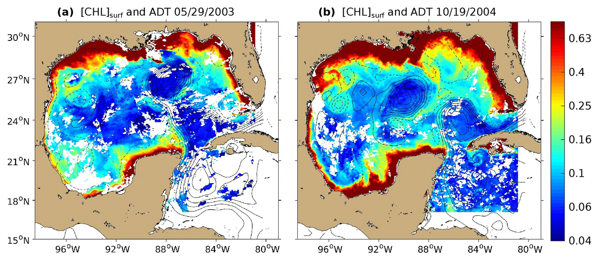
Figure 1The 8 d composite images of [Chl]surf (in mg m−3) around (a) 29 May 2003 and (b) 19 October 2004 derived from Aqua-MODIS images overlaid with contours of absolute dynamic topography (ADT; in m) derived from Aviso images are superimposed. Contour interval is 10 cm, and ADT values lower than 40 cm are shown with dashed curves.
2.2 Observational data set used
Satellite observations are used to evaluate the ability of GOLFO12-PISCES to reproduce the dynamical and biological signatures associated with LCEs. Surface geostrophic velocities are derived from a ∘ multi-satellite merged product of absolute dynamic topography (ADT) provided by AVISO+ (http://marine.copernicus.eu, last access: 10 April 2021). Surface chlorophyll concentrations are from the Aqua-MODIS 4 km product (Sathyendranath et al., 2012; http://marine.copernicus.eu, last access: 10 April 2021) and consist of 8 d composites from 2003 to 2015.
2.2.1 LCEs detection, tracking, and composite construction
In order to track the LCEs, we use the algorithm developed by Nencioli et al. (2010), which has been extensively employed to track coherent mesoscale eddies (Dong et al., 2012; Ciani et al., 2017; Zhao et al., 2018) and submesoscale eddies (Damien et al., 2017). It is based on the geometric organization of the velocity fields, dominated by rotation, that develop around eddy centers. Here, it is applied to weekly AVISO+ surface geostrophic velocities and GOLFO12-PISCES 5 d averaged velocities at 20 m depth. The selection of LCEs is defined using the criteria that eddies have to be shed from the Loop Current.
In order to assess the [Chl] response to LCE dynamics, eddy-centric horizontal images and transects of LCEs are used to make composites constructed by averaging modeled variables of the different LCEs collocated to their center. The transect building procedure involves an axisymmetric averaging that assumes axis symmetry of the dynamical structures and no tilting of their rotation axis. Moreover, we choose not to consider the LCEs formation period and the LCEs destruction period when reaching the western basin (Lipphardt et al., 2008; Hamilton et al., 2018) as LCE destruction and formation involves specific processes (Frolov et al., 2004; Donohue et al., 2016). We therefore focus on the LCEs contained in the central part of the GoM from 86 to 94∘ W. Annual composites are computed along with monthly composite averages in order to assess seasonal variability. Composite LCEs averaged during the months of January and February are referred to as winter composites, and those averaged during July and August are referred to as summer composites. These composites provide an overview of the LCEs mean hydrographical, biogeochemical, and dynamical characteristics.
2.2.2 Diagnostics
The LCE radius RLCE is estimated as the radial distance between the center and the peak azimuthal velocity Vmax. The mixed layer depth (MLD), a major physical factor influencing nutrient distribution and [Chl] dynamics (Mann and Lazier, 2006), is defined as the depth at which potential density exceeds its value at 10 m depth by 0.125 kg m−3 (Levitus, 1982; Monterey and Levitus, 1997).
The stratification of the water column is evaluated by the square of the buoyancy frequency , where g is the gravitational acceleration, z is depth, ρ is density, and ρ0 is a reference density.
As carried out in Damien et al. (2018), several metrics are defined and used to describe [Chl]:
- –
[Chl]surf is [Chl] averaged between 0 and 30 m depth and considered as surface concentration (in mg Chl m−3).
- –
[Chl]tot is the integrated content of [Chl] over the 0–350 m layer (in mg Chl m−2).
- –
DCM is the depth of the deep chlorophyll maximum (in m).
- –
[Chl]DCM is the [Chl] value at DCM depth (in mg Chl m−3).
To understand the mesoscale distribution of [Chl], key biological variables are vertically integrated between 0 and 350 m: the phytoplanktonic concentration [Phy]tot, the primary production rate PPtot, and the grazing rate GRZtot. PPtot consists of two components: new production PPNtot fueled by nutrients supplied from a source external to the mixed layer and regenerated production PPRtot sustained by recycled nutrients within the euphotic layer (Dugdale and Goering, 1967; Eppley and Peterson, 1979). The euphotic depth corresponds to 1 % of the incoming photosynthetic active radiation at surface and reaches between 120 and 150 m in the GoM (Jolliff et al., 2008; Linacre et al., 2019). A chlorophyll concentration anomaly within LCEs, [Chl]′, is computed as , where is the averaged background [Chl] field in the open GoM waters (for radius > 250 km from the LCEs' centers). We also define the normalized anomaly as , with SD the standard deviation operator, following a similar approach as Gaube et al. (2013, 2014) and Dufois et al. (2016). To limit the influence of very high [Chl] values in coastal waters under the direct influence of continental discharges, a salinity filtering criterion (lower than 36 psu) is applied. A similar method was used by Gaube et al. (2013, 2014) to filter edge effects but using a distance criterion instead.
3.1 Satellite observations of [Chl]
Figure 1 shows the 8 d averaged satellite observations of the surface chlorophyll around 29 May 2003 (panel a) and 19 October 2004 (panel b). These observations highlight the strong contrast between the eutrophic conditions in the coastal waters and the oligotrophic conditions in the open ocean, as already addressed by several studies (Martinez-Lopez and Zavala-Hidalgo, 2009; Pasqueron de Fommervault et al., 2017). Far from the coast, these figures also reveal that the surface chlorophyll varies at a scale of the order of 100 km with a distribution that tends to follow the absolute dynamic topography (ADT) contours.
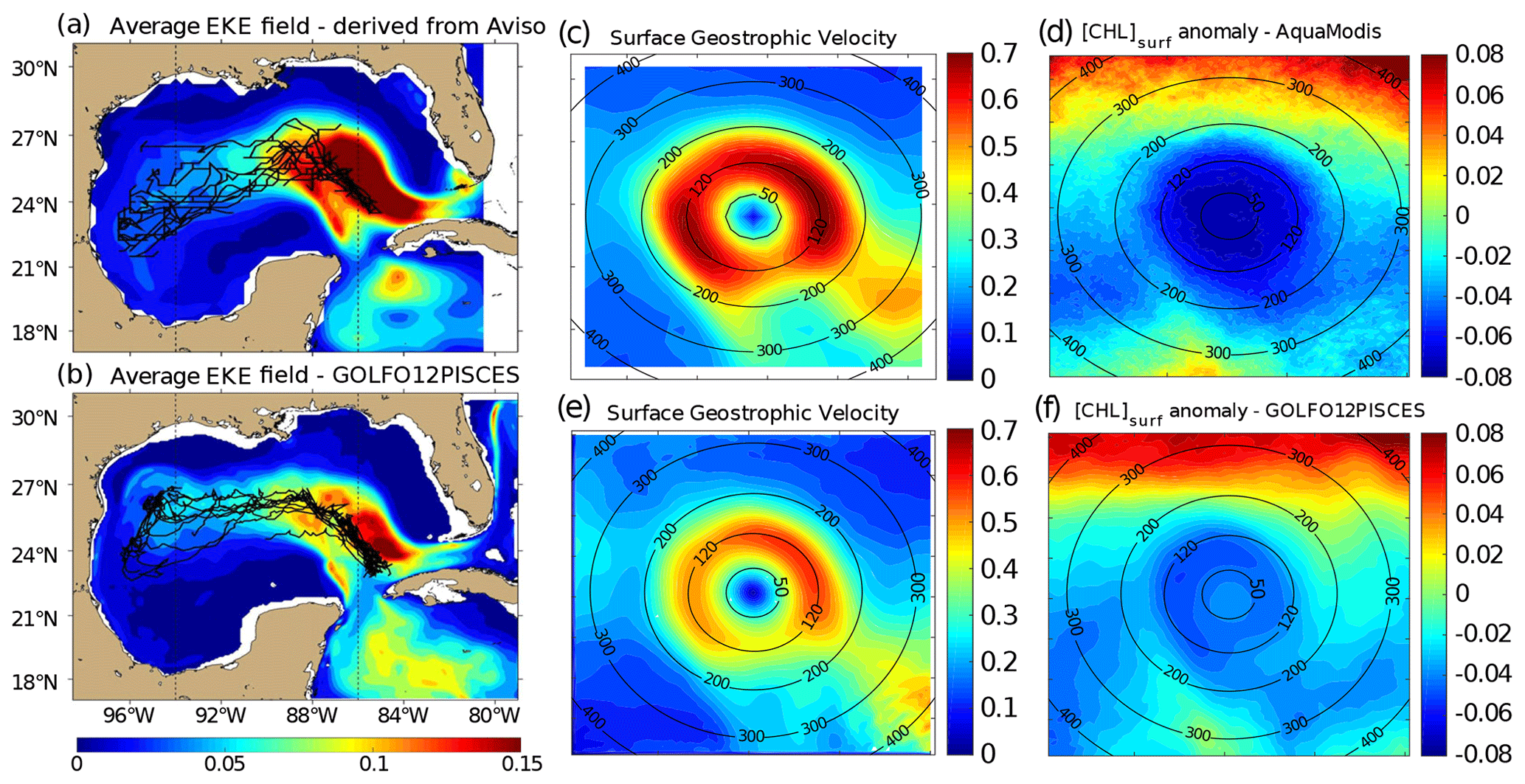
Figure 2Average eddy kinetic energy (EKE) field derived from (a) Aviso geostrophic surface velocities and from (b) GOLFO12-PISCES currents at 10 m depth. The trajectories of the tracked LCEs are superimposed to the EKE field (black lines). Dashed vertical black lines indicate the central GoM area over which composites are built. Annual LCE composite images of surface geostrophic velocities for (c) Aviso images and (e) GOLFO12-PISCES. Annual LCE composite images of surface chlorophyll concentration anomaly for (d) MODIS images, and (f) GOLFO12-PISCES. Black circles indicate the radius in kilometers.
LCE trajectories are reported in Fig. 2a, superimposed onto the geostrophic climatological eddy kinetic energy (EKE) field at the surface. EKE is computed from eddy velocities defined on each grid cell as the difference between the total horizontal current and its mean value over 120 d. This time window is chosen to filter the seasonal signal. EKE is concentrated in the Loop Current (LC) and on the westward pathway of the LCEs (Lipphardt et al., 2008) demonstrating that LCEs constitute the major source of EKE in the GoM open waters (Sheinbaum et al., 2016; Sturges and Leben, 2000; Hamilton, 2007; Jouanno et al., 2016).
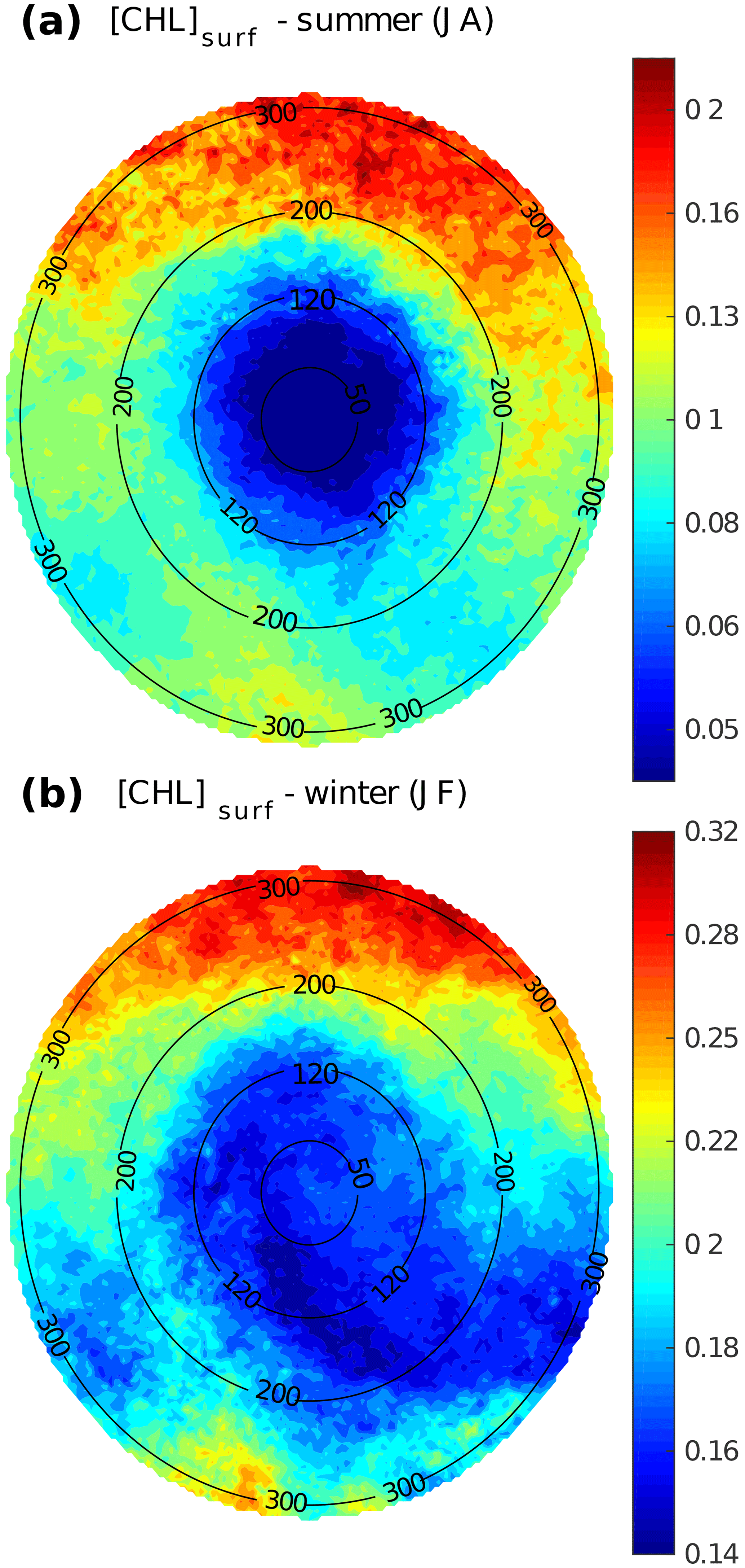
Figure 3LCE composite images of [Chl]surf derived from Aqua-MODIS for the (a) summer and (b) winter seasons. Black circles indicate the radius in kilometers.
LCE annual composites of surface geostrophic velocities (Fig. 2c) and [Chl]surf (Fig. 2d) are built from 482 different satellite images. On average, we found that RLCE is ∼ 120 km and Vmax ∼ 0.6–0.7 m s−1, in agreement with previously reported LCEs (Elliot, 1982; Cooper et al., 1990; Forristal et al., 1992; Glenn and Ebbesmeyer, 1993; Weisberg and Liu, 2017; Tenreiro et al., 2018). LCEs are associated with a negative [Chl]surf anomaly (∼ −0.07 mg m−3 in the annual average). The LCEs' influence on [Chl]surf is largest in summer (Fig. 3a) when it reaches very low values (< 0.045 mg m−3), which correspond to an anomaly of ∼ −0.08 mg m−3. This anomaly is less remarkable in winter (∼ −0.06 mg m−3; Fig. 3b) when [Chl]surf is ∼ 0.17 mg m−3 within LCEs. The high chlorophyll concentrations in the northern part of the composites (in the southern part too but in smaller proportions) are related to shelves.
3.2 Dynamical characterization of modeled LCEs
A total of 11 model LCEs were detected during the 5 years of simulation. Their trajectories are reported in Fig. 2b, superimposed upon the climatological EKE field simulated at 10 m. The westward–southwestward propagation of LCEs is well reproduced (Vukovich, 2007) even though the LCE translation is almost westward in GOLFO12-PISCES. A comparison with Fig. 2a shows the ability of GOLFO12-PISCES to represent the mean and transient dynamical features of the GoM open waters (also see Garcia-Jove et al., 2016).
The robustness of the composite method arises from the number of LCEs used to build the composites:
-
Annual composite is built from 605 5 d averaged LCE model outputs from 10 different LCEs.
-
Summer composite is built from 83 5 d averaged LCE model outputs from 8 different LCEs.
-
Winter composite is built from 93 5 d averaged LCE model outputs from 9 different LCEs.
The model LCE surface geostrophic velocities (Fig. 2e) have important similarities with velocities inferred from altimetry (Fig. 2c), confirming that GOLFO12-PISCES reproduces the surface signature of the LCEs. However, one can also notice an underestimation of the surface orbital velocities (∼ 25 % on average over the 50–200 km radius range). This bias could result from the relatively coarse model resolution and 5 d output frequency that are unable to fully capture the gradient intensity at RLCE. The assumption of an axial symmetry of the LCE circulation around its center also induces an error that tends to decrease Vmax.
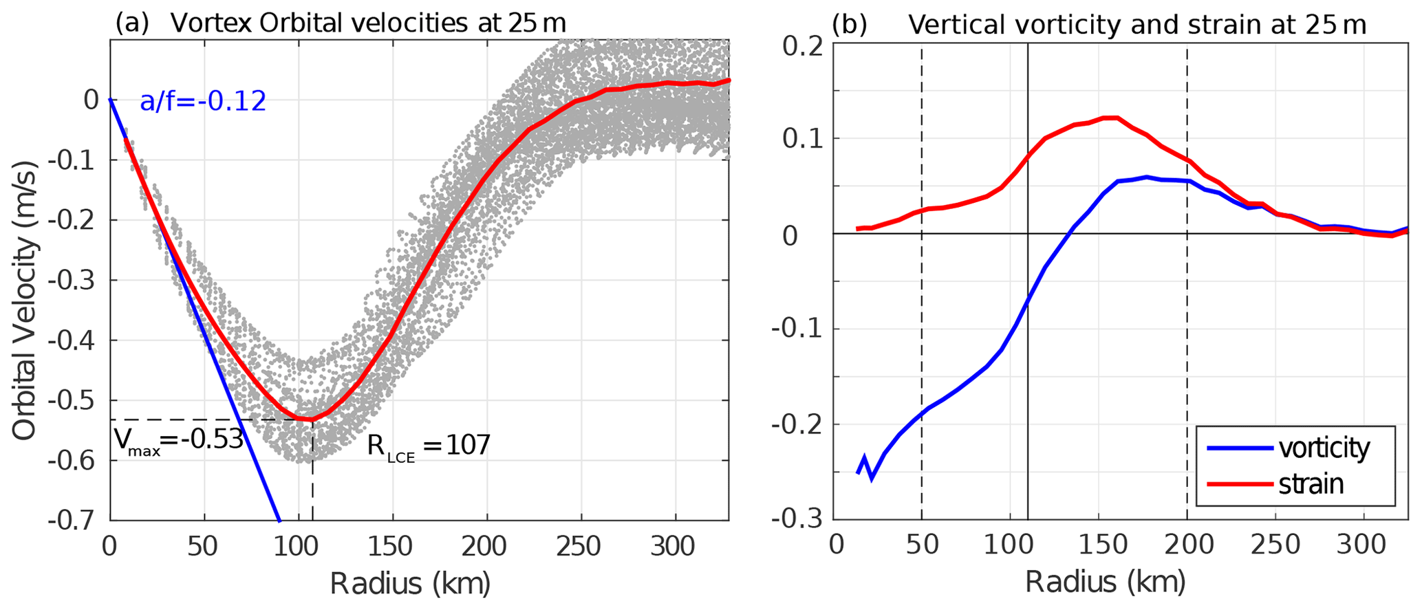
Figure 4(a) Orbital velocities at 25 m depth as a function of the radius of each detected LCE (light gray dots). The red line is the LCE orbital velocity profile of the annually averaged composite. (b) Vertical vorticity and strain computed from the averaged orbital velocity profile assuming no radial velocity in cylindrical coordinates as and .
Orbital velocities of composite eddies are used to distinguish different dynamical areas within LCEs. The model annual average dynamical profile at 25 m depth (Fig. 4) reveals a typical vortex-like structure with RLCE∼107 km and Vmax∼0.53 m s−1 and suggests the following decomposition:
-
r<50 km is the LCE core where the eddy is approximately in solid body rotation: , where the coefficient a is related to the Rossby number (). The ratio is estimated to be (Fig. 4). In this field, the strain is reduced to a minimum and the flow is dominated by rotation.
-
km is the LCE ring structure where the orbital velocity reaches its maximum at RLCE and then decreases. The horizontal strain is important in this field, even dominating vorticity from radius exceeding RLCE.
-
r>200 km is the background GoM where the velocity anomalies related to the LCEs vanish.
In the vertical (Fig. 5a), LCEs are near-surface intensified anticyclonic vortex rings. At depth, the orbital peak velocity decreases rapidly. At 500 m depth, Vmax is ∼0.17 m s−1 and RLCE∼75 km, and the dynamical LCE signal nearly vanishes below 1500 m depth (Vmax<0.03 m s−1). The proposed division into three distinct dynamical regions applies from the surface down to 500 m depth (Fig. 5a).
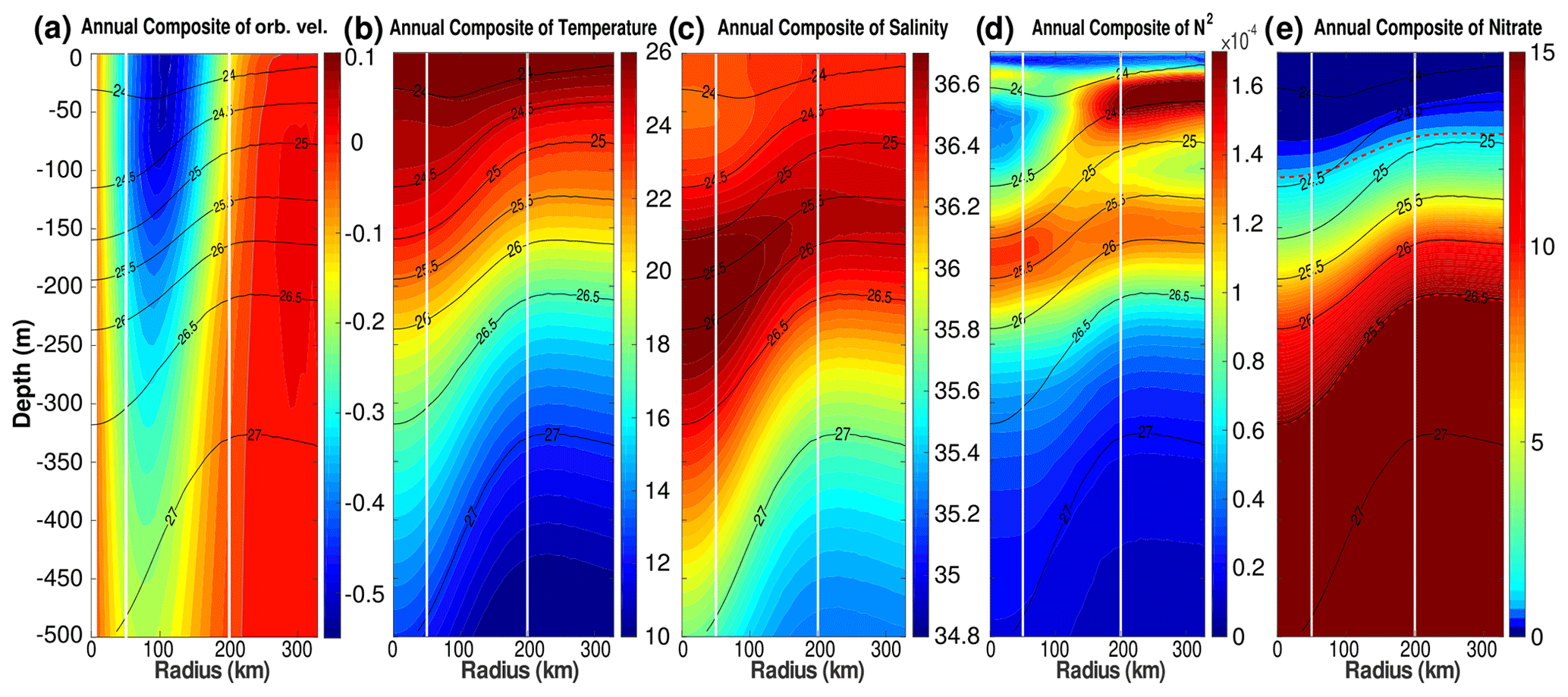
Figure 5Annually averaged LCE composite transects of (a) orbital velocities (m s−1), (b) potential temperature (∘C), (c) salinity (psu), (d) squared Brunt–Väisälä frequency (N2 in s−2), and (e) nitrate concentration (mmol m−3). Isopycnal anomalies (black contours) are superimposed on all panels. Vertical white lines delimit the three dynamical fields of the LCE composite. (e) Dashed red lines highlight two specific iso-nitrate contours: 1 and 15 mmol m−3.
The composite hydrological structure of modeled LCEs is shown in Fig. 5b and c. The depression of isopycnals, associated with a depression of isotherms and isohalines, is characteristic of oceanic anticyclones. In the core of the eddies, the composite depicts a salinity maximum located between 100 and 300 m, corresponding to the signature of the Atlantic Subtropical Underwater (ASTUW) of Caribbean origin entering the GoM through the Yucatán Channel (Badan et al., 2005; Hernandez-Guerra and Joyce, 2000; Wuust, 1964). This salinity maximum is not limited to the core of the LCE but gradually erodes and shallows: 36.82 psu at 200 m in the LCE core and 36.61 psu at 150 m in the background GoM common water. Details on the fate of this salinity maximum investigated with GOLFO12 simulations can be found in Sosa-Gutiérrez et al. (2020). The ASTUW layer (salinity > 36.5 psu) is also thicker in the LCE core (∼ 190 m thick) compared to the background GoM water (∼ 120 m thick). Overall, GOLFO12-PISCES reproduces the observed hydrological structure of LCEs (Elliott, 1982; LeHenaff et al., 2012; Hamilton et al., 2018; Meunier et al., 2018b).
The annually averaged LCE composite presents a lens-shaped structure exhibiting a ∼ 50 m thick layer of weakly stratified waters located between 50 and 100 m depth (Fig. 5d). This subsurface modal water presents hydrological characteristics close to the observed background GoM waters (potential temperature ∼ 25.4 ∘C and salinity ∼ 36.3 psu; Meunier et al., 2018b) and is surrounded below and above by well-stratified layers (Meunier et al., 2018a). The upper pycnocline varies seasonally and vanishes in winter due to the deepening of the mixed layer, whereas the lower pycnocline is permanent.
The downward displacement of isopycnals is accompanied by a depletion of nutrients in the upper layer of the LCE core (Fig. 5e). This is a typical feature of mesoscale anticyclones in the ocean (McGillicuddy et al., 1998; Oschlies and Garcon, 1998). The 1 mmol m−3 iso-nitrate concentration (hereafter , sometimes referred to as the nitracline as in Cullen and Eppley, 1981, Pasqueron de Fommervault et al., 2017, and Damien et al., 2018) is located at ∼ 70 m depth in the background GoM waters, whereas it is found much deeper in the core ( m). At depth, iso-nitrate layers and isopycnals are well correlated (Ascani et al., 2013; Omand and Mahadevan, 2015). For instance, iso-nitrate concentration of 15 mmol m−3 follows the displacements of the 1026.5 kg m−3 isopycnal. However, above 150 m, the density/nitrate relation is different inside and outside the eddies ( is collocated with isopycnal 1024.4 kg m−3 in the LCE core and with isopycnal 1024.9 kg m−3 in the background GoM).

Figure 6LCE composite transects of [Chl] during summer season (a) and winter season (b). Density anomalies (black contours) are superimposed. Vertical white lines delimit the three dynamical fields of the LCE composite. For each season, [Chl] profiles in the LCE core (r<50 km, red lines) and in the background GoM (200 km < r<330 km, gray lines) are plotted. Key metrics concerning [Chl] profiles are also indicated in the tables.
3.3 Surface and vertical distribution of chlorophyll in LCEs
The large difference in stratification between the LCE core and background GoM suggests a contrasted seasonal response of the [Chl]. This is evidenced by the analysis of summer and winter composites of [Chl] vertical distribution.
In summer (Fig. 6a), [Chl]surf is ∼ 30 % lower in the LCE core (r<50 km) than in the background GoM (200 km < r<330 km). A pronounced DCM, characteristic of oligotrophic environments, is deeper in the core (∼ 97 m) than in the background GoM (∼ 69 m) with chlorophyll concentrations significantly lower in the interior ( %).
In winter, the [Chl] is maximum at the surface in all the composite domains (Fig. 6b). [Chl]surf is lower in the LCE core compared to the background GoM, but the difference is less marked ( %) than in summer. The main discrepancy is the depth of the inflection point of these profiles. It is deeper in the LCE core (150 m), resulting in a more homogenized [Chl] over a deeper layer than in the background GoM ( m).
However, despite reduced surface concentration both in winter and summer, the integrated chlorophyll content, [Chl]tot, shows a distinct seasonal pattern compared to the surface (Tables in Fig. 6).
In summer, [Chl]tot is lower in the LCE core (27.58 mg m−2) compared to the background GoM (29.41 mg m−2), and Δ[Chl] mg m−2.
In winter, [Chl]tot is higher in the LCE core (44.98 mg m−2) compared to the background GoM (38.03 mg m−2), and Δ[Chl] mg m−2.
The winter increase in [Chl]tot is around 29 % in the background GoM, whereas it reaches 63 % in the LCE core, leading to [Chl]tot in the core being larger than [Chl]tot in the background GoM in winter. Meanwhile, [Chl]surf remains lower within the LCE core. The fact that the [Chl] at the surface does not reflect its depth-integrated behavior means that the peculiar variability in [Chl] within LCEs may not be fully captured by ocean color satellite measurements. This is consistent with the observations and modeling results of Pasqueron de Fommervault et al. (2017) and Damien et al. (2018) which addressed the vertical [Chl] distribution in the GoM.
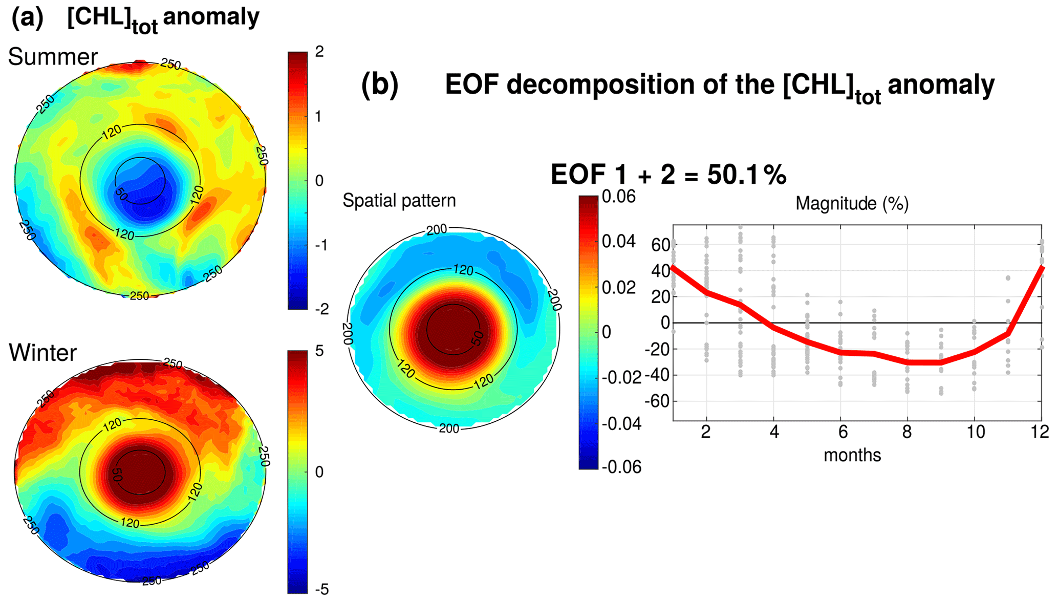
Figure 7(a) Anomaly of [Chl]tot in summer and winter seasons. Black circles indicate the radius in kilometers. (b) EOF decomposition of the normalized [Chl]tot anomaly. The spatial patterns and monthly magnitude (gray dots; the red line represents their monthly averaged value) of the two first modes are indicated. Modes 1 and 2 were summed together and represent 50.1 % of the total variance.
[Chl]tot is strongly shaped by both the seasonal variability and the LCEs. The seasonal composites of [Chl]tot, shown in Fig. 7a, confirm the summer/winter contrast and highlight a monopole structure with a relatively homogeneous distribution of [Chl]tot within the eddy's core. In order to better characterize the spatiotemporal variability in [Chl]tot induced by LCEs, an empirical orthogonal function (EOF) analysis was performed on the normalized [Chl]tot anomaly (Fig. 7b) following the methodology of Dufois et al. (2016). It consists of decomposing the signal into orthogonal modes of variability. Here, we choose to focus on the first two most significant modes which explain 40.2 % and 9.9 % of the variability. Since they both depict a similar monopole structure in the LCE core, they were added up in a mode referred to as EOF 1+2 that is responsible for 50 % of the total [Chl]tot variance within LCEs. The third eigenmode (not shown) accounts for 6.2 % and depicts a dipole structure with opposite polarity located at the east and north of the eddy center. On average, the EOF 1+2 mode is positive in winter (from December to March) and negative the rest of the year (from April to November), with a maximum in December and January and a minimum in September. This justifies, a posteriori, the choice to consider winter and summer LCE composites.
The composite evolution of the LCE [Chl]tot along their westward journey is shown in Fig. 8a and b. It illustrates how the total chlorophyll concentration is preferentially increased in winter within the LCE core as soon as the LCEs are shed from the LC. The winter [Chl]tot within LCEs is much larger (exceeding 1 standard deviation) than the background winter [Chl]tot. In terms of integrated [Chl], the LCE-induced seasonal variability overwhelms the GoM open-water background seasonal variability.
In an oligotrophic environment such as the GoM open waters, the primary production is generally limited by nutrient supply, and [Chl]tot exhibits low seasonal variability at the GoM basin scale (Pasqueron de Fommervault et al., 2017). The winter increase in [Chl]tot within the LCE core (which translates into an effective increase in biomass; see Appendix A) contrasts with and may have large implications for the regional biogeochemical cycles and ecosystem structuration. It also echoes several studies which report elevated [Chl]surf within anticyclonic eddies in the oligotrophic subtropical gyre of the southeastern Indian Ocean (Martin and Richards, 2001; Waite et al., 2007; Gaube et al., 2013; Dufois et al., 2016, 2017; He et al., 2017), questioning the classical paradigm of low productivity usually associated with anticyclonic eddies.
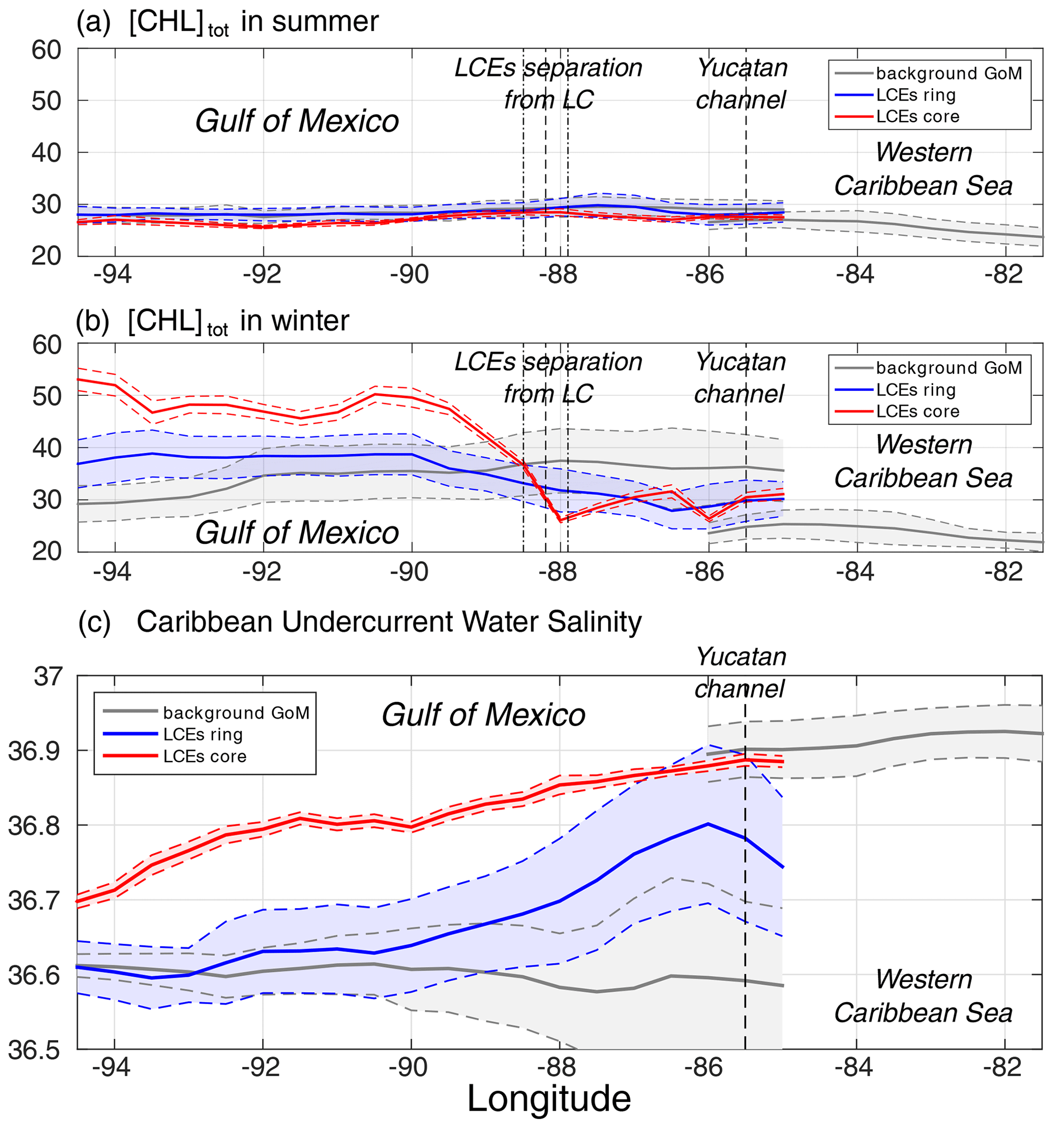
Figure 8(a) Summer [Chl]tot, (b) winter [Chl]tot, and (c) salinity of Caribbean waters (ASTUW defined as the subsurface salinity maximum) as a function of longitude in (red) the LCE core, in (blue) the LCE ring, and in (gray) the background GoM. Full lines indicate the averaged value and dashed lines the ± 1 standard deviation interval.
The mechanisms explaining the LCE impact on [Chl] are discussed below, trying to rationalize the respective role of abiotic (e.g., trapping, winter mixing, Ekman pumping) and biotic processes (e.g., primary production, PP, grazing pressure, regenerated versus new PP).
4.1 Eddy trapping
The distinct hydrological and biogeochemical properties associated with the LCE core suggest their ability to trap and transport oceanic properties. This mechanism, known as the eddy trapping (Early et al., 2011; Lehahn et al., 2011; McGillicuddy, 2015; Gaube et al., 2017), is efficient only if the orbital velocities of the vortex are faster than the eddy propagation speed (Flierl, 1981; d'Ovidio et al., 2013). The rotational velocities of the model LCEs are ∼ 0.53 m s−1 and 1 order of magnitude larger than the propagation velocities (∼ 0.046 m s−1 on average). This suggests that LCEs might have a certain ability to trap the water masses present in their core with relatively low exchanges with the exterior.
Salinity is well-suited to investigate water masses trapped within the LCE core during their propagation toward the western GoM (Fig. 8c; Sosa-Gutierez et al., 2020): salinity distribution shows a marked subsurface maximum that is not affected by biogeochemical processes. In the western Caribbean Sea, ASTUW is characterized by high salinity (∼ 36.9 psu on average) and low standard deviation (<0.05 psu). The eastern GoM salinity field reveals that most of the ASTUW crosses the Yucatán Channel within the Loop Current. During the formation of LCEs, a significant part of ASTUW is captured in the LCE core with low alteration of its properties (Figs. 5c and 8c). Within the LCE core, the water mass is transported from the eastern to the western GoM where its salinity decreases from 36.9 to 36.7 psu. Although altered, the ASTUW signature is still clearly detectable in the GoM western boundary. The other part of ASTUW entering the GoM is found in the LCE ring. Compared to the core, the salinity in the ring is on average lower (∼ 36.8 psu in the eastern GoM) and presents a high standard deviation, pointing out that more recent ASTUW co-exists with older ASTUW that yields lower salinity maxima. As LCEs travel westward across the GoM, salinity in the LCE ring decays rapidly to reach values similar to the background GoM values (∼ 36.6 psu). This homogenization mainly arises from vertical mixing and winter mixed layer convection (Sosa-Gutierez et al., 2020). Horizontal intrusions and filamentation may also contribute to this homogenization (Meunier et al., 2020). The composites also suggest that almost no ASTUW enters the GoM apart from the LCEs. The slight increase in the background salinity from the eastern to western GoM is a consequence of the diffusion of salt from the LCEs toward the exterior.
Although LCEs undergo considerable decaying rates, their erosion is particularly strong in the ring, while the core remains better isolated from the surrounding waters (Lehahn et al., 2011; Bracco et al., 2017). Since no significant [Chl]tot seasonal variability is reported in the western Caribbean Sea (Fig. 8), the biogeochemical behavior in the LCE core then has to be driven by local processes with the low influence of the horizontal advective process from the ring or of the Caribbean waters trapped during the LCE formation. Given that the LCE core is also quite homogeneous, the following discussion relies on the analysis of the seasonal cycles of selected parameters averaged within the LCE core.
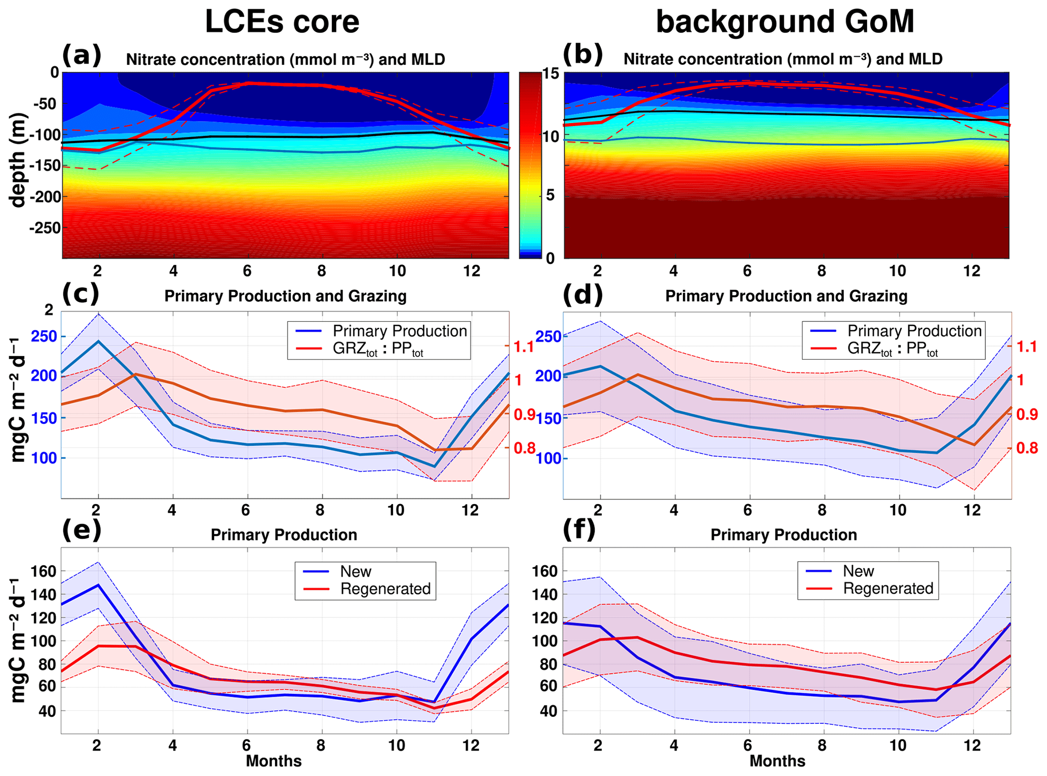
Figure 9Climatological seasonal cycles of (a, b) nitrate concentration profiles (the red line overlaid is the average mixed layer depth, the blue line is the base of the euphotic layer, and the black line is the nitracline), (c, d) the total primary production (blue) and the ratio of grazing rate over primary production (red), and (e, f) the new (blue) and regenerated (red) primary production. Panels (a, c, e) refer to the seasonal time series in the LCE core (r<50 km), whereas the right panels (b, d, f) refer to the seasonal time series in the background GoM (r>200 km). For each average cycle, the mean value is shown (full line) along with its variability (±1 standard deviation relative to the mean, dashed lines).
4.2 Nitracline depth and nutrient supply into the mixed layer
The LCEs impact the upper ocean stratification (Fig. 5d), the nutricline depth (Fig. 5e), and consequently the nutrient supply to the euphotic layer (McGillicuddy et al., 2015). The relationship between mixed layer deepening and nutrient supply is studied here by comparing the with the MLD (Fig. 9a, b).
In late-spring and summer (from May to September), the water column is stratified (shallow MLD), and the downward displacement of the isopycnals within the LCEs pushes nutrients below the euphotic zone (see also Figs. 5e, 6a): less nutrients are available within the LCE cores for phytoplankton growth, explaining a deeper and less intense DCM. In winter, the convective mixing, fostered both by intense buoyancy losses and strong mechanical energy input at the surface, causes a larger deepening of the mixed layer within the LCE core ( m; Fig. 9a) compared to the background ( m; Fig. 9b). This asymmetry is due to a pronounced decrease in the surface and subsurface stratification within the LCE core (Fig. 5d; see also Kouketsu et al., 2012). A quantitative diagnostic of the stratification is given by the columnar buoyancy, , which measures the buoyancy loss required to mix the water column to a depth H (Herrmann et al., 2008). Figure 10a reveals significant differences in pre-winter buoyancy between the eddy core and its surroundings. Assuming that the change in buoyancy content is mainly controlled by the buoyancy flux at the surface (see Turner, 1973; Lascaratos and Nittis, 1998), it suggests that mixing the water column down to m depth requires smaller surface buoyancy loss in LCE cores compared to the background GoM (Fig. 10b).
However, the larger winter deepening of the mixed layer within the LCE core is not a sufficient condition to explain a larger nutrient supply. Indeed, it fosters the transport of nutrients from the nitracline toward the mixed layer because both are getting closer. Figure 10c highlights that a smaller buoyancy loss mixes down the water column to greater nutrient concentration levels in the LCE core compared to the LCEs surrounding it. This likely explains the winter increase in surface nitrate concentration within the LCEs (Fig. 9a). In addition, a diagnostic of the different contributions to [NO3] evolution is proposed in Appendix B. It shows the dominant role of vertical advection and diffusion in winter in providing nutrients to the euphotic layer in the LCE core.

Figure 10(a) Columnar buoyancy transect composite in summer, corresponding to pre-winter mixing season. Iso-nitrate concentrations (black contours) are superimposed. Vertical white lines delimit the three dynamical fields of the LCE composite. (b) Vertical increase in the columnar buoyancy in the LCE core versus the background GoM. Colors refer to depth. (c) Columnar buoyancy loss required to mix the water column down to the iso-nitrate surface defined by the line color.
So far we have assumed that the surface buoyancy fluxes are identical over the LCE core and the background GoM. However, this is not strictly the case because temperature and/or salinity features in the LCEs and background waters are different (Fig. 5b, c; see also Williams, 1988). The modeled surface buoyancy loss during the winter season is ∼18 % more intense within the LCEs. This difference is substantial and probably mainly driven by additional surface cooling applied to the warm LCE core through air–sea interaction. It contributes to enhance convection within the eddy's core and then nutrient supply toward the surface.
4.3 Productivity and grazing
The primary productivity PPtot presents a clear seasonal cycle both in the LCE cores and in the background GoM with lower values in October–November, a sharp increase starting in November, a maximum in February, and a gradual decrease from March to October (Fig. 9c, d). The annual PPtot is slightly lower in the LCE core (∼142.4 mg C m−2 d−1) than in the background GoM (∼ 148.9 mg C m−2 d−1). The amplitude of the seasonal cycle is larger in the LCE core: from April to November, PPtot is on average ∼ 12 % lower in the LCE core, whereas, in winter, PPtot is ∼ 14 % higher and reaches ∼ 243.2 mg C m−2 d−1 in February. Particularly in the LCE core, the PPtot seasonal cycle is tightly correlated with vertical mixing, revealing the important role of mixing in the biogeochemistry. The relatively low standard deviation of the monthly PPtot distribution in the LCE core also supports the idea that the influence of the seasonal variability in the forcing largely overwhelms their interannual and sub-monthly variability (Fig. 9c).
The ratio of the PPNtot and PPRtot provides information about the mechanisms controlling the biomass growth (Fig. 9e, f). In winter, the PPNtot plays a leading role, reaching up to 113–147 mg C m−2 d−1, driven by the winter mixing and induced [NO3] fluxes (see Appendix B). Conversely, the PPRtot is dominant from April to October. During this period, low NO3 resources are available in the euphotic layer, and the ecosystem preferentially uses ammonium to sustain the PPtot. This seasonal pattern is characteristic of oligotrophic environments such as the GoM open waters (Wawrik et al., 2004; Linacre et al., 2015). In winter, changes in PPtot are correlated with the intensity of winter mixing in the LCE core (Fig. 9c) and the background GoM (Fig. 9d). The larger PPNtot in the eddy core is consistent with a larger supply of [NO3] and is evidence that the core of anticyclones can be preferential spots of enhanced biological production.
The pressure exerted by zooplankton grazers varies seasonally (Fig. 9c, d). It shows a similar seasonal cycle in the LCE core and in the background GoM. On average, ∼ 90 % of the total growth is consumed by grazers, reaching the highest impact in March, just one month after the peak season of the PPtot in both areas. In February the difference between the primary production and the grazing rate tends to be larger in the LCE core (GRZtot PP) than in the GoM background (GRZtot PP; Fig. 9c), leading to an enhanced net primary production. Considering the ecosystem from a “top-down” perspective, the grazing rate also participates then in enhancing [Chl]tot within the LCE core compared to the background.
4.4 Eddy–wind interactions
In summer, the total primary production is higher in the background GoM waters as the regenerated production rate is higher. Since grazing is known to be a major contributor of the recycling loop in the euphotic zone (Sherr and Sherr, 2002), the lower grazing rate inside the LCE during summer (Fig. 9c, d) likely explains this lower regenerated production. In addition, the biogeochemical consumption of nitrate that fosters the production of organic matter occurs in a deeper layer within the LCE core compared to the background GoM (Fig. B1e, f). It is then more likely exported out of the euphotic layer in the form of a settling particle, leading to lower remineralization rates in the upper layers to feed regenerated production. More surprising, the new primary production exhibits similar rates in both regions, although NO3 depletion occurs deeper in the LCE core. In the absence of a strong enough vertical mixing when the mixed layer is shallow, this apparent mismatch requires an additional mechanism, vertical advection, capable of supplying NO3 to the euphotic layer (Sweeney et al., 2003; McGillicuddy et al., 2015).
The model vertical velocity in the LCEs reveals an upward pumping in their core (Fig. 11). The vertical velocity between 100 and 500 m is on average + 0.07 m d−1. This vertical transport is mainly driven by two mechanisms, eddy pumping (Falkowski et al., 1991) and eddy–wind interaction (Dewar and Flierl, 1987), but their relative importance is difficult to quantify (Gaube et al., 2014; McGillicuddy et al., 2015).
The eddy pumping mechanism is related to the decay of the rotational velocities from the moment LCEs are released from the Loop Current. In the LCE core, this decay is considered as moderate since lateral diffusivity is expected to be relatively low (Sect. 4.1). This process may however be considerable in the LCE ring where the erosion rates are important (Meunier at al., 2020).
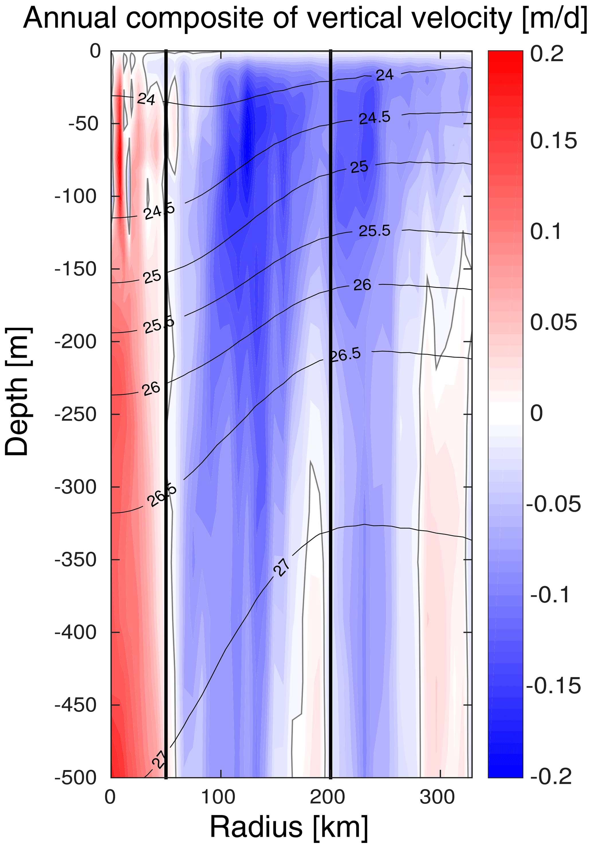
Figure 11Annually averaged LCE composite transects of vertical velocities (m d−1). Isopycnals anomalies (black contours) are superimposed on all panels. Vertical white lines delimit the three dynamical fields of the LCE composite.
Eddy–wind interactions are due to mesoscale modulation of the Ekman transport so that they are often qualified as eddy-Ekman pumping (He et al, 2017). Following the observation of an LCE core in quasi-solid body rotation, the horizontal vorticity varies little with the radius resulting in a negligible “non-linear” contribution of the Ekman pumping (McGillicuddy et al., 2008; Gaube et al., 2015). Assuming a small effect of the eddy SST-induced (sea surface temperature) Ekman pumping, the total Ekman pumping simplifies into its “linear” contribution, computed as , where ρ0 is the surface density, f the Coriolis parameter, τ the stress at the sea surface depending on both the wind and ocean currents at the surface (Martin and Richards, 2001, their Eq. 12), and ∇× the curl operator. Considering uniform wind velocities ranging from 4.5 to 7.5 m s−1 (Nowlin and Parker, 1974; Passalacqua et al., 2016) blowing over the LCE, the curl of the stress arises from the anticyclonic surface circulation generated by the eddy. Its manifestation is a persistent horizontal divergence at surface balanced by an upward pumping in the eddy interior (see Martin and Richards, 2001; Gaube et al., 2013, 2014, for further details). With ρ0∼1023 kg m−3 and s−1, we estimate WE to range from + 0.06 to 0.13 m d−1, in agreement with the modeled vertical velocity within the core. The eddy-Ekman pumping mechanism could explain a large fraction of the gradual upwelling within the eddy's core (Fig. 11) and may actively contribute to the advective vertical flux of nutrients (see Appendix B). In summer, this mechanism could explain why new primary production rates are similar in the LCE core and the background GoM waters, although the nutrient pool is located much deeper in the LCE core.
The eddy-Ekman pumping persists in the LCE core throughout its lifetime as long as there is a wind stress applied at the surface. During wintertime, we expect that both vertical mixing and eddy-Ekman pumping participate to increase the new primary production. A question then arises about the relative contribution of winter mixing to eddy-Ekman pumping in the LCE core primary production increase in winter. This issue was tackled by He et al. (2017) and Travis et al. (2020) comparing the rate of change in the mixed layer depth with the vertical velocity induced by the eddy-Ekman pumping (Eq. 4 in He et al, 2017). In the GoM, even if the wind shows larger magnitudes in winter, it is also associated with a large variability. As a consequence, the variability in Ekman pumping is also found to be large, and a robust seasonal cycle which would allow us to isolate the Ekman pumping in winter cannot be clearly identified. However, in the LCE core, we estimate the mixed layer to deepen at roughly 0.8 m d−1, which is on average about 1 order of magnitude larger than the higher bound of the estimated pumping mechanism typically occurring in winter in response to stronger wind events. This supports winter mixing as the overwhelming process for the LCE-induced primary production peak in winter.
The [Chl] variability induced by the mesoscale Loop Current eddies in the Gulf of Mexico is studied by analyzing vortex composite fields generated from a coupled physical–biogeochemical model at ∘ horizontal resolution. LCEs are hotspots for mesoscale biogeochemical variability. Despite the [Chl]surf negative anomaly associated with their core (r<50 km), model results indicate that LCEs are associated with enhanced phytoplankton biomass content, particularly in winter. This enhancement results from the contribution of multiple mechanisms of physical–biogeochemical interactions and contrasts with the background oligotrophic surface waters of the GoM.
The main results of this study are the following:
-
LCE cores present a negative surface chlorophyll anomaly.
-
Unlike [Chl]surf, [Chl]tot is larger in the LCE cores compared to the background GoM in winter.
-
LCE cores trigger a large phytoplankton biomass increase in winter.
-
The winter mixing is a key mesoscale mechanism that preferentially supplies nutrients to the euphotic layer within the LCE core. Consequently, it drives an eddy-induced peak of new primary production.
-
Eddy-Ekman pumping is a significant mechanism for sustaining relatively high new primary production rates within LCE cores during summer.
The phytoplankton biomass increase in individual LCE cores suggests that LCEs play an important role in sustaining the large-scale GoM productivity.
GOLFO12-PISCES provides numerical results which largely conformed to observations. This extensive validation gives confidence about its ability to produce realistic seasonal and mesoscale variability in biogeochemical tracers at surface and subsurface, in particular the one associated with LCEs. However, biases are inherent to the model and might affect the main conclusions drawn. For example, in situ measurements reveal an intense variability in [Chl] vertical profiles in winter that the model tends to underestimate (Green et al., 2014; Damien et al., 2018). In particular, some individual observed profiles in winter present a DCM, while GOLFO12-PISCES largely favors well-mixed [Chl] profiles. The under-representation of these profiles, potentially due to a relatively coarse model resolution, could be associated with an underestimation of [Chl]tot in winter. The results exposed in this study would require further confirmation, notably by more subsurface in situ measurements, in particular within the core of LCEs where no [Chl] profiles were observed in winter.
Although the biological response to LCEs may present some specificities due to the particular dynamical nature of LCEs, this study suggests potentially generic insights on the biogeochemical role that anticyclonic eddies could play in oligotrophic environments. It echoes the previous works of Martin and Richards (2001), Gaube et al. (2014, 2015), and especially Dufois et al. (2014, 2016) and He et al. (2017) who proposed winter vertical mixing as an explanation for the positive [Chl]surf anomaly observed in anticyclones in the southern Indian Ocean. One of the most crucial points to be underlined from our results is that the enhanced primary production and biomass content within anticyclonic eddies may not necessarily be correlated with the surface layer variability. In oligotrophic areas, the integrated content of chlorophyll in the water column has to be considered. This implies that caution should be exercised in the analysis and interpretation of [Chl]surf observed by remote sensing instruments and highlights the crucial need for in situ biogeochemical and bio-optical measurements. In oligotrophic environments, defined by their low production rates and their low chlorophyll concentration, anticyclonic eddies are able to trigger local enhanced biological productivity and generate phytoplankton biomass positive anomalies. In a scenario of expansion of oligotrophic areas (Barnett et al., 2001; Behrenfeld et al., 2006; Polovina et al., 2008), the fate and role of mesoscale anticyclones is an important aspect to be considered.
This study focuses on mesoscale physical–biogeochemical interactions, which is the spectral range resolved by the GOLFO12-PISCES configuration. It is evidence of the important role of mixing in primary production in the LCE core at seasonal scale. However, mixing also presents significant fluctuations at higher frequencies, associated with particular atmospheric events like storms. The PPtot response to such forcing requires further investigation to verify if the correlation between PPtot and mixing still holds at higher frequencies where other additional drivers might also become important. For instance, the role of submesoscale is of particular interest since it has been proven to trigger mechanisms of significant importance for biogeochemistry (Lévy et al., 2018). Higher model resolutions can locally enhance density gradients (Lévy et al., 2012; Omand et al., 2015) leading to ageostrophic circulations that perturb the circular flow around vortices (Martin and Richards, 2001) or enhanced vertical velocities that potentially foster the nutrient supply to the euphotic layer. Beside the mesoscale Ekman pumping located at the eddy center, eddy–wind interactions also produce vertical velocities at the eddy periphery (e.g., Flierl and McGillicuddy, 2002). Finally, it is also worth noting that anticyclonic mesoscale eddies are capable of trapping near-inertial energy waves in the ocean (Kunze, 1985; Danioux et al., 2008; Koszalka et al., 2010; Pallas-Sanz et al., 2016) where they produce vertical recirculation patterns (Zhong and Bracco, 2013). Even if some of these dynamical aspects are partially resolved at ∘ horizontal resolution, higher resolutions simulations with higher frequency outputs are necessary to correctly assess their specific impact.
[Chl] is widely used as a proxy for photosynthetic biomass (Strickland, 1965; Cullen, 1982). However, in addition to depending on phytoplankton concentration, it is also affected by several other factors mainly produced by intracellular physiological mechanisms (Geider, 1987). In particular, photoacclimation processes have been proven to be determinant to explain [Chl]surf variability in oligotrophic areas (Mignot et al., 2014). In the GoM open waters, this issue was specifically addressed at a basin scale in Pasqueron de Fommervault et al. (2017) considering in situ particulate backscattering measurements and in Damien et al. (2018) from modeling tools. They both reach the same conclusion: [Chl]tot variability provides a reasonably good estimate of the total C biomass variability ([Phy]tot).
This is confirmed by the small amplitude of the seasonal cycle of the ratio [Chl]tot [Phy]tot in the background GoM (0.256±0.004 g mol−1 averaged throughout the year; Fig. A1). In the LCE core, this statement is still valid but must be qualified since the ratio [Chl]tot [Phy]tot presents small but significant changes through the year (Fig. A1a). It is around 0.24 g mol−1 from March to November and increases sharply in December to reach about 0.32 g mol−1 in January and February. As a result, in winter, the photoacclimation mechanism accounts for ∼ 25 % of the total [Chl]tot increase (the remaining part being an effective phytoplankton biomass increase). In summer, the ratio [Chl]tot [Phy]tot is slightly lower in the LCE core compared to the background GoM. As a consequence, the [Chl]tot negative anomaly associated with the LCE core does not necessarily translate into a [Phy]tot negative anomaly.
Overall in the GoM open waters, there is a dominance of the small-size phytoplankton over the large-size class in proportions close to 80 % : 20 % (Linacre et al., 2015). Although the modeled ecosystem structure is relatively simple, this typical community size structure is well reproduced by GOLFO12-PISCES (Fig. A1c and d), which also suggests a shift in the ecosystem structure in winter. The different response among size classes results from the enhancement of nutrient vertical flux. The role of “secondary” nutrients in this change in the community composition must also not be overlooked, in particular for diatoms (accounted in the model's large-size group) since they also uptake silicate (Benitez-Nelson et al., 2007). Moreover, GOLFO12-PISCES exhibits a modulation of the ecosystem structure by LCEs. The dominance of small-size phytoplankton is slightly more marked in summer, and the winter shift is stronger in the LCE core.

Figure A1Climatological seasonal cycles of (a, b) the -biomass ratio and (c, d) the vertically integrated content of phytoplankton concentration (small size in blue, large size in red). Panels (a, c) refer to the time series in the LCE core (r<50 km), whereas (b, d) refer to the time series in the background GoM (r>200 km). For each average cycle, the average value is shown (full line) along with its variability (±1 standard deviation relative to the mean, dashed lines).
Nutrient availability in the euphotic layer is a key mechanism to trigger biomass increase in LCEs. The processes driving the seasonality of nutrient concentrations are here investigated to diagnose the different contributions to nitrate concentration (hereafter [NO3]) variability. The goal is to confirm the vertical transport of nutrients and quantify the budget in order to determine the driving mechanisms. The analysis is restricted to nitrate concentrations, considered as the main limiting factor for large-size-class phytoplankton growth in the GoM (Myers et al., 1981; Turner et al., 2006), although phosphates and silicates are also modeled. We do not exclude the possibility that phosphates or silicates could also play a significant role. In cylindrical coordinates, the [NO3] equation reads as follows:
Basically, this is a 3D advection and diffusion equation with added “sources and sinks” terms, namely biogeochemical release and uptake rates. One must include also an “Asselin term”, a modeling artifact due to the Asselin time filtering. We focus on the seasonal cycle of three particular trend terms: the vertical mixing (Fig. B1a, b), the vertical advection (Fig. B1c, d), and a “source minus sink” term (Fig. B1e, f).
The [NO3] variations from vertical dynamics are mainly positive, especially in the first 100 m of the water column. This translates into a year-round [NO3] source driven by physical processes. By contrast, biogeochemical processes consume NO3 in the upper layer to sustain the primary production (Fig. B1e, f). In the subsurface layer (∼ below the isoline on which nitrate concentration is equal to 2 mmol m−3), the process of nitrification constitutes a biological source of [NO3]. Firstly, this represents the global functioning of the ecosystem, valid in both fields and throughout the year. However, the seasonal cycle strongly influences the magnitude of these trend terms, in particular in the LCE core.
In winter, from December to February, vertical advective and diffusive motions produce an increase in [NO3] within the mixed layer. This tendency consists in an advective entrainment resulting from the deepening of the mixed layer which mainly acts to increase [NO3] at the base of the mixed layer (Fig. B1c, d) and vertical mixing which redistributes vertically the nutrients and tends to homogenize [NO3] in the mixed layer (Fig. B1a, b). The winter [NO3] increase is most important in the LCE core at the base of the mixed layer ( mmol m−3 d−1, nearly 3 times larger than in the background GoM), attesting here to a preferential NO3 uplift due to deeper convection. Integrated over the mixed layer, the winter vertical fluxes produce [NO3] enhancement of mmol m−2 d−1 in the eddy core, whereas it is only of mmol m−2 d−1 in the background GoM. This also explains why, on average, the density–nitrate relation differs in the LCE core (Fig. 5e). In response, the [NO3] tendency due to biogeochemical processes indicates an increase in the [NO3] uptake. This increase is about 1.5 times larger in the core ( mmol m−2 d−1 integrated over the mixed layer) than in the background GoM ( mmol m−2 d−1). Knowing that it feeds biomass production, this [NO3] loss is consistent with the primary production peak in winter (Fig. 9e, f).
In summer, [NO3] variations due to vertical processes are smaller than in winter. They are also weaker in the LCE core upper layer (almost nil in the 0–50 m layer) compared to the background GoM, consistent with a deeper NO3 pool and a shallow mixer layer. In the eddy core, one can assume that the NO3 vertical supply is entirely consumed before reaching 50 m. Below 50 m, vertical [NO3] diffusive trends are consistently more important in the background GoM, in agreement with a steeper nitracline (Fig. 5e). In contrast, vertical [NO3] advective trends in the eddy core are similar to or can eventually exceed the trends in the background GoM (as in September and October for example). This confirms a pumping mechanism to sustain primary production in summer within the eddy core (Sect. 4.4). The biogeochemical activity related to [NO3] variations is also less intense in summer compared to winter. The depth of maximum [NO3] uptake is located just above the DCM and [NO3] release below. The loss of [NO3] is about twice as large in the background GoM ( mmol m−3 d−1) than in the LCE core ( mmol m−3 d−1). It is noteworthy that the biogeochemical [NO3] source term, namely the nitrification rate, is really low within the eddy core.
To close this analysis of the [NO3] budget, it must be said that lateral diffusion and Asselin tendencies are marginal terms compared to the others. Horizontal advection is of the same order of magnitude as the vertical terms and mainly acts to redistribute horizontally the vertically moved NO3 (see Supplement Sect. S1).
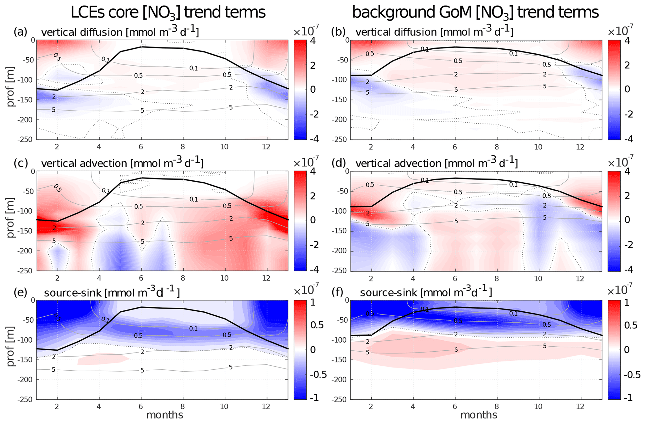
Figure B1Seasonal cycle of nitrate trend terms in the (a, c, e) LCE core and in the (b, d, f) background GoM. The trend induced by (a, b) vertical mixing, the (c, d) vertical advection, and the (e, f) biogeochemical source minus sink is represented. Isopycnal anomalies (gray contours) and the depth of the mixed layer (black line) are superimposed.
The NEMO ocean engine code (Madec et al., 2019) used in this study is accessible at a public repository: https://doi.org/10.5281/zenodo.1464816 (last access: 14 July 2021) . The PISCES-v2 code is described in Aumont et al. (2015).
Data from the model simulation used in this study are available upon request to the corresponding author.
The supplement related to this article is available online at: https://doi.org/10.5194/bg-18-4281-2021-supplement.
PD, JS, and OPdF conceptualized the analysis and developed the methodology. PD did the formal analysis. PD, JS, JJ, and OD developed the numerical simulation. PD did the writing and original draft preparation. All authors provided feedback on the analysis and interpretation of results and contributed to reviewing and editing the manuscript. JS acquired funding of this research. All authors have read and agreed to the published version of the manuscript.
The authors declare that they have no conflict of interest.
Publisher’s note: Copernicus Publications remains neutral with regard to jurisdictional claims in published maps and institutional affiliations.
We acknowledge PEMEX's specific request to the hydrocarbon fund to address the environmental effects of oil spills in the Gulf of Mexico. We acknowledge the provision of supercomputing facilities by CICESE.
This research has been supported by the National Council of Science and Technology of Mexico (CONACYT) – Mexican Ministry of Energy (SENER) Hydrocarbon Trust (project no. 201441) and a contribution of the Gulf of Mexico Research Consortium (CIGoM).
This paper was edited by Kenneth Rose and reviewed by Z. George Xue and one anonymous referee.
Ascani, F., Richards, K. J., Firing, E., Grant, S., Johnson, K. S., Jia, Y., Lukas, R., and Karl, D. M.: Physical and biological controls of nitrate concentrations in the upper subtropical North Pacific Ocean, Deep Sea Res. Pt. II, 93, 119–134, 2013.
Aumont, O. and Bopp, L.: Globalizing results from ocean in situ iron fertilization studies, Global Biogeochem. Cy., 20, GB2017, https://doi.org/10.1029/2005GB002591, 2006.
Aumont, O., Ethé, C., Tagliabue, A., Bopp, L., and Gehlen, M.: PISCES-v2: an ocean biogeochemical model for carbon and ecosystem studies, Geosci. Model Dev., 8, 2465–2513, https://doi.org/10.5194/gmd-8-2465-2015, 2015.
Badan, Jr., A., Candela, J., Sheinbaum, J., and Ochoa, J.: Upper-layer circulation in the approaches to Yucatan Channel, Washington DC American Geophysical Union Geophysical Monograph Series, 161, 57–69, 2005.
Barnett, T. P., Pierce, D. W., and Schnur, R.: Detection of anthropogenic climate change in the world's oceans, Science, 292, 270–274, 2001.
Behrenfeld, M. J., O'Malley, R. T., Siegel, D. A., McClain, C. R., Sarmiento, J. L., Feldman, G. C., Milligan, A. J., Falkowski, P. G., Letelier, R. M., and Boss, E. S.: Climate-driven trends in contemporary ocean productivity, Nature, 444, 752–755, 2006.
Benitez-Nelson, C. R., Bidigare, R. R., Dickey, T. D., Landry, M. R., Leonard, C. L., Brown, S. L., Nencioli, F., Rii, Y. M., Maiti, K., Becker, J. W., and Bibby, T. S.: Mesoscale eddies drive increased silica export in the subtropical Pacific Ocean, Science, 316, 1017–1021, 2007.
Biggs, D. C. and Ressler, P. H.: Distribution and abundance of phytoplankton, zooplankton, ichthyoplankton, and micronekton in the deepwater Gulf of Mexico, Gulf of Mexico Science, 19, 2, https://doi.org/10.18785/goms.1901.02, 2001.
Bracco, A., Provenzale, A., and Scheuring, I.: Mesoscale vortices and the paradox of the plankton, P. Roy. Soc. B-Bio., 267, 1795–1800, 2000.
Brodeau, L., Barnier, B., Treguier, A.-M., Penduff, T., and Gulev, S: An ERA40-based atmospheric forcing for global ocean circulation models, Ocean Model, 31, 88–104, https://doi.org/10.1016/j.ocemod.2009.10.005, 2010.
Brokaw, R. J., Subrahmanyam, B., and Morey, S. L.: Loop current and eddy driven salinity variability in the Gulf of Mexico, Geophys. Res. Lett., 46, 5978–5986, https://doi.org/10.1029/2019GL082931, 2019.
Chelton, D., DeSzoeke, R., Schlax, M., El Naggar, K., and Siwertz, N.: Geographical variability of the first baroclinic Rossby radius of deformation, J. Phys. Oceanogr., 28, 433–460, 1998.
Ciani, D., Carton, X., Aguiar, A. B., Peliz, A., Bashmachnikov, I., Ienna, F., Chapron, B., and Santoleri, R.: Surface signature of Mediterranean water eddies in a long-term high-resolution simulation, Deep Sea Res. Pt. I, 130, 12–29, 2017.
Cooper, C., Forristall, G. Z., and Joyce, T. M.: Velocity and hydrographic structure of two Gulf of Mexico warm-core rings, J. Geophys. Res.-Oceans, 95, 1663–1679, 1990.
Cullen, J. J. and Eppley, R. W.: Chlorophyll maximum layers of the Southern-California Bight and possible mechanisms of their formation and maintenance, Oceanol. Ac., 4, 23–32, 1981.
Cullen, J. J.: The deep chlorophyll maximum: Comparing vertical profiles of chlorophyll a, Can. J. Fish. Aquat. Sci., 39, 791–803, 1982.
Dai, A. and Trenberth, K. E.: Estimates of freshwater discharge from continents: Latitudinal and seasonal variations, J. Hydrometeorol., 3, 660–687, 2002.
Damien, P., Bosse, A., Testor, P., Marsaleix, P., and Estournel, C.: Modeling Postconvective Submesoscale Coherent Vortices in the Northwestern M editerranean Sea, J. Geophys. Res-Ocean., 122, 9937–9961, https://doi.org/10.1002/2016JC012114, 2017.
Damien, P., Pasqueron de Fommervault, O., Sheinbaum, J., Jouanno, J., Camacho-Ibar, V. F., and Duteil, O.: Partitioning of the Open Waters of the Gulf of Mexico Based on the Seasonal and Interannual Variability of Chlorophyll Concentration, J. Geophys. Res.-Oceans, 123, 2592–2614, 2018.
Danioux, E., Klein, P., and Rivière, P.: Propagation of wind energy into the deep ocean through a fully turbulent mesoscale eddy field, J. Phys. Oceanogr., 38, 2224–2241, 2008.
Dewar, W. and Flierl G.: Some effects of the wind on rings, J. Phys. Oceanogr., 17, 1653–1667, 1987.
Doney, S. C., Glover, D. M., McCue, S. J., and Fuentes, M.: Mesoscale variability of Sea-viewing Wide Field-of-view Sensor (SeaWiFS) satellite ocean color: Global patterns and spatial scales, J. Geophys. Res.-Oceans, 108, 3024, https://doi.org/10.1029/2001JC000843, 2003.
Dong, C., Lin, X., Liu, Y., Nencioli, F., Chao, Y., Guan, Y., Chen, D., Dickey, T., and McWilliams, J. C. : Three-dimensional oceanic eddy analysis in the Southern California Bight from a numerical product, J. Geophys. Res., 117, C00H14, https://doi.org/10.1029/2011JC007354, 2012.
Donohue, K. A., Watts, D. R., Hamilton, P., Leben, R., and Kennelly, M.: Loop current eddy formation and baroclinic instability, Dyn. Atmos. Oceans, 76, 195–216, 2016.
d'Ovidio, F., De Monte, S., Della Penna, A., Cotté, C., and Guinet, C.: Ecological implications of eddy retention in the open ocean: a Lagrangian approach, J. Phys. A Math. Theor., 46, 254023, https://doi.org/10.1088/1751-8113/46/25/254023, 2013.
Dufois, F., Hardman-Mountford, N. J., Greenwood, J., Richardson, A. J., Feng, M., Herbette, S., and Matear, R.: Impact of eddies on surface chlorophyll in the South Indian Ocean, J. Geophys. Res.-Oceans, 119, 8061–8077, 2014.
Dufois, F., Hardman-Mountford, N. J., Greenwood, J., Richardson, A. J., Feng, M., and Matear, R. J.: Anticyclonic eddies are more productive than cyclonic eddies in subtropical gyres because of winter mixing, Sci. Adv., 2, e1600282, https://doi.org/10.1126/sciadv.1600282, 2016.
Dufois, F., Hardman-Mountford, N. J., Fernandes, M., Wojtasiewicz, B., Shenoy, D., Slawinski, D., Gauns., M., Greenwood., J., and Toresen, R.: Observational insights into chlorophyll distributions of subtropical South Indian Ocean eddies, Geophys. Res. Lett., 44, 3255–3264, 2017.
Dugdale, R. C. and Goering, J. J. :Uptake of new and regenerated forms of nitrogen in primary productivity, Limnol. Oceanogr., 12, 196–206, 1967.
Early, J. J., Samelson, R. M., and Chelton, D. B.: The evolution and propagation of quasigeostrophic ocean eddies, J. Phys. Oceanogr., 41, 1535–1555, 2011.
Elliott, B. A.: Anticyclonic rings in the Gulf of Mexico, J. Phys. Oceanogr., 12, 1292–1309, 1982.
Eppley, R. W. and Peterson B. J.: Particulate organic matter flux and planktonic new production in the deep ocean, Nature, 282, 677–680, 1979.
Falkowski, P., Ziemann, D., Kolber, Z., and Bienfang, P.: Role of eddy pumping in enhancing primary production in the ocean, Nature, 352, 55–58, 1991.
Flierl, G. R.: Particle motions in large-amplitude wave fields, Geophys. Astro. Fluid, 18, 39–74, 1981.
Flierl, G. R. and McGillicuddy, D. J.: Mesoscale and submesoscale physical-biological interactions, The Sea, 12, 113–185, 2002.
Forristall, G. Z., Schaudt, K. J., and Cooper, C. K.: Evolution and kinematics of a Loop Current eddy in the Gulf of Mexico during 1985, J. Geophys. Res.-Oceans, 97, 2173–2184, 1992.
Frolov, S. A., Sutyrin, G. G., Rowe, G. D., and Rothstein, L. M.: Loop Current eddy interaction with the western boundary in the Gulf of Mexico, J. Phys. Oceanogr., 34, 2223–2237, 2004.
Garcia, H. E., Locarnini, R. A., Boyer, T. P., Antonov, J. I., Baranova, O. K., Zweng, M. M., and Johnson D. R.: World Ocean Atlas 2009, in: Dissolved oxygen, apparent oxygen utilization, and oxygen saturation (NOAA Atlas NESDIS 70, edited by: Levitus, S., Vol. 3, Washington, DC: U.S. Government, Printing Office, 344 pp., 2010.
Garcia-Jove Navarro, M., Sheinbaum Pardo, J., and Jouanno, J.: Sensitivity of Loop Current metrics and eddy detachments to different model configurations: The impact of topography and Caribbean perturbations, Atmosfera, 29, 235–265, https://doi.org/10.20937/ATM.2016.29.03.05, 2016.
Garçon, V. C., Oschlies, A., Doney, S. C., McGillicuddy, D., and Waniek, J.: The role of mesoscale variability on plankton dynamics in the North Atlantic, Deep Sea Res. Pt. II, 48, 2199–2226, 2001.
Gaube, P., Chelton, D. B., Strutton, P. G., and Behrenfeld, M. J.: Satellite observations of chlorophyll, phytoplankton biomass, and Ekman pumping in nonlinear mesoscale eddies, J. Geophys. Res.-Oceans, 118, 6349–6370, 2013.
Gaube, P., McGillicuddy, D. J., Chelton, D. B., Behrenfeld, M. J., and Strutton, P. G.: Regional variations in the influence of mesoscale eddies on near-surface chlorophyll, J. Geophys. Res.-Oceans, 119, 8195–8220, 2014.
Gaube, P., Chelton, D. B., Samelson, R. M., Schlax, M. G., and O'Neill, L. W.: Satellite observations of mesoscale eddy-induced Ekman pumping, J. Phys. Oceanogr., 45, 104–132, 2015.
Geider, R. J.: Light and temperature dependence of the carbon to chlorophyll a ratio in microalgae and cyanobacteria: implications for physiology and growth of phytoplankton, New Phytol., 106, 1–34, 1987.
Glenn, S. M. and Ebbesmeyer C. C.: Drifting buoy observations of a loop current anticyclonic eddy, J. Geophys. Res., 98, 20, https://doi.org/10.1029/93JC02078, 1993.
Green, R. E., Bower, A. S., and Lugo-Fernández, A.: First autonomous bio-optical profiling float in the Gulf of Mexico reveals dynamic biogeochemistry in deep waters, PLOS ONE, 9, e101658, https://doi.org/10.1371/journal.pone.0101658, 2014.
Guo, M., Xiu, P., Li, S., Chai, F., Xue, H., Zhou, K., and Dai, M.: Seasonal variability and mechanisms regulating chlorophyll distribution in mesoscale eddies in the South China Sea, J. Geophys. Res.-Oceans, 122, 5329–5347, https://doi.org/10.1002/2016JC012670, 2017.
Hamilton, P.: Eddy statistics from Lagrangian drifters and hydrography for the northern Gulf of Mexico slope, J. Geophys. Res., 112, C09002, https://doi.org/10.1029/2006JC003988, 2007.
Hamilton, P., Leben, R., Bower, A., Furey, H., and Pérez-Brunius, P.: Hydrography of the Gulf of Mexico Using Autonomous Floats, J. Phys. Oceanogr., 48, 773–794, https://doi.org/10.1175/JPO-D-17-0205.1, 2018.
He, Q., Zhan, H., Shuai, Y., Cai, S., Li, Q. P., Huang, G., and Li, J.: Phytoplankton bloom triggered by an anticyclonic eddy: The combined effect of eddy Ekman pumping and winter mixing, J. Geophys. Res.-Oceans, 122, 4886–4901, 2017.
Hernandez-Guerra, A. and Joyce, T. M.: Water masses and circulation in the surface layers of the Caribbean at 66 W, Geophys. Res. Lett., 27, 3497–3500, https://doi.org/10.1029/1999GL011230, 2000.
Herrmann, M., Somot, S., Sevault, F., Estournel, C., and Deque, M.: Modeling the deep convection in the northwestern Mediterranean Sea using an eddy-permitting and an eddy-resolving model: Case study of winter 1986–1987, J. Geophys. Res., 113, C04011, https://doi.org/10.1029/2006JC003991, 2008.
Huang, J. and Xu, F: Observational evidence of subsurface chlorophyll response to mesoscale eddies in the North Pacific, Geophys. Res. Lett., 45, 8462–8470, https://doi.org/10.1029/2018GL078408, 2018.
Jolliff, J. K., Kindle, J. C., Penta, B., Helber, R., Lee, Z., Shulman, I., Arnone, R., and Rowley, C. D.: On the relationship between satellite-estimated bio-optical and thermal properties in the Gulf of Mexico, J. Geophys. Res., 113, G01024, https://doi.org/10.1029/2006JG000373, 2008.
Jouanno, J., Ochoa, J., Pallàs-Sanz, E., Sheinbaum, J., Andrade-Canto, F., Candela, J., and Molines, J. M.: Loop current frontal eddies: Formation along the Campeche Bank and impact of coastally trapped waves, J. Phys. Oceanogr., 46, 3339–3363, https://doi.org/10.1175/JPO-D-16-0052.1, 2016.
Klein, P. and Lapeyre, G.: The oceanic vertical pump induced by mesoscale and submesoscale turbulence, Annu. Rev. Mar. Sci., 1, 351–375, 2009.
Koszalka, I. M., Ceballos, L., and Bracco, A.: Vertical mixing and coherent anticyclones in the ocean: the role of stratification, Nonlinear Process. Geophys., 17, 37–47, 2010.
Kouketsu, S., Tomita, H., Oka, E., Hosoda, S., Kobayashi, T., and Sato, K.: The role of meso-scale eddies in mixed layer deepening and mode water formation in the western North Pacific, in: New Developments in Mode-Water Research, Springer, Tokyo, 59–73, 2011.
Kunze, E.: Near-inertial wave propagation in geostrophic shear, J. Phys. Oceanogr., 15, 544–565, 1985.
Lascaratos, A. and Nittis, K.: A high-resolution three-dimensional numerical study of intermediate water formation in the Levantine Sea, J. Geophys. Res., 103, 18497–18511, 1998.
Lehahn, Y., d'Ovidio, F., Lévy, M., Amitai, Y., and Heifetz, E.: Long range transport of a quasi isolated chlorophyll patch by an Agulhas ring, Geophys. Res. Lett., 38, L16610, https://doi.org/10.1029/2011GL048588, 2011.
Le Hénaff, M., Kourafalou, V. H., Morel, Y., and Srinivasan, A.: Simulating the dynamics and intensification of cyclonic Loop Current Frontal Eddies in the Gulf of Mexico, J. Geophys. Res.-Oceans, 117, C02034, https://doi.org/10.1029/2011JC007279, 2012.
Levitus, S.: Climatological atlas of the world ocean (NOAA Prof. Pap. 13), Washington, DC: U.S. Government Printing Office, 173 pp., 1982.
Lévy, M., Ferrari, R., Franks, P. J., Martin, A. P., and Rivière, P.: Bringing physics to life at the submesoscale. Geophys. Res. Lett., 39, L14602, https://doi.org/10.1029/2012GL052756, 2012.
Lévy, M., Franks, P. J. S., and Mith, K. S.: The role of submesoscale currents in structuring marine ecosystems, Nat. Commun., 9, 4758, https://doi.org/10.1038/s41467-018-07059-3, 2018.
Linacre, L., Lara-Lara, R., Camacho-Ibar, V., Herguera, J. C., Bazán-Guzmán, C., and Ferreira-Bartrina, V.: Distribution pattern of picoplankton carbon biomass linked to mesoscale dynamics in the southern gulf of Mexico during winter conditions, Deep Sea Res. Pt. I, 106, 55–67, 2015.
Linacre L., Durazo, R., Camacho-Ibar, V. F., Selph, K. E., Lara-Lara, J. R., Mirabal-Gómez, U., Bazán-Guzmán, C., Lago-Lestón, A., Fernández-Martín, E. M., and Sidón-Ceseña, K.: Picoplankton Carbon Biomass Assessments and Distribution of Prochlorococcus Ecotypes Linked to Loop Current Eddies During Summer in the Southern Gulf of Mexico, J. Geophys. Res.-Oceans, 124, 8342–8359, 2019.
Lipphardt, B., Poje, A. C., Kirwan, A., Kantha, L., and Zweng, M.: Death of three Loop Current rings, J. Mar. Res., 66, 25–60, 2008.
Madec, G.: NEMO ocean engine, Note Du Pole De Modelisation (Vol. 27), Paris, France: Institut Pierre-Simon Laplace, 406 pp., 2016.
Madec, G., Bourdallé-Badie, R., Chanut, J., Clementi, E., Coward, A., Ethé, C., Iovino, C., Lea, D., Lévy, C., Lovato, T., Martin, N., Masson, S., Mocavero, S., Rousset, C., Storkey, D., Vancoppenolle, M., Müeller, S., Nurser, G., Bell, M., and Samson, G.: NEMO ocean engine (Version v4.0), Notes Du Pôle De Modélisation De L'institut Pierre-simon Laplace (IPSL), Zenodo [Dataset], https://doi.org/10.5281/zenodo.1464816 (last access: 14 July 2021), 2019.
Mann, K. H. and Lazier, J. R. N.: Dynamics of marine ecosystems (3 Edn.), Oxford, UK: Blackwell Publishing, 512 pp., 2006.
Mahadevan, A.: Ocean science: Eddy effects on biogeochemistry, Nature, 506, 168–169, https://doi.org/10.1038/nature13048, 2014.
Martin, A. P. and Richards, K. J.: Mechanisms for vertical nutrient transport within a North Atlantic mesoscale eddy, Deep Sea Res. Pt. II, 48, 757–773, 2001.
Mayot, N., D'Ortenzio, F., Taillandier, V., Prieur, L., de Fommervault, O. P., Claustre, H., Bosse, A., Testor, P., and Conan, P.: Physical and biogeochemical controls of the phytoplankton blooms in North Western Mediterranean Sea: A multiplatform approach over a complete annual cycle (2012–2013 DEWEX experiment), J. Geophys. Res.-Oceans, 122, 9999–10019, 2017.
McClain, C. R., Signorini, S. R., and Christian, J. R.: Subtropical gyre variability observed by ocean-color satellites, Deep Sea Res. Pt. II, 51, 281–301, 2004.
McGillicuddy Jr., D. J.: Mechanisms of Physical-Biological-Biogeochemical Interaction at the Oceanic Mesoscale, Annu. Rev. Mar. Sci., 8, 125–159, https://doi.org/10.1146/annurev-marine-010814-015606, 2016.
McGillicuddy Jr., D. J., Robinson, A. R., Siegel, D. A., Jannasch, H. W., Johnson, R., Dickey, T. D., McNeil, J., Michaels, A. F., and Knap, A. H.: Influence of mesoscale eddies on new production in the Sargasso Sea, Nature, 394, 263–266, https://doi.org/10.1038/28367, 1998.
McGillicuddy Jr., D. J. and Robinson, A. R.: Eddy-induced nutrient supply and new production in the Sargasso Sea, Deep Sea Res. Pt. I, 44, 1427–1450, 1997.
Meunier, T., Tenreiro, M., Pallàs-Sanz, E., Ochoa, J., Ruiz-Angulo, A., Portela, E., Cusí, S., Damien, P., and Carton, X.: Intrathermocline eddies embedded within an anticyclonic vortex ring, Geophys. Res. Lett., 45, 7624–7633, https://doi.org/10.1029/2018GL077527, 2018a.
Meunier, T., Pallás-Sanz, E., Tenreiro, M., Rodriguez, E. P., Ochoa, J., Ruiz-Angulo, A., and Cusí, S.: The Vertical structure of a Loop Current Eddy, J. Geophys. Res.-Oceans, 123, 6070–6090, https://doi.org/10.1029/2018JC013801, 2018b.
Meunier, T., Sheinbaum, J., Pallàs-Sanz, E., Tenreiro, M., Ochoa, J., Ruiz-Angulo, A., Carton, X., and de Marez, C.: Heat Content Anomaly and Decay of Warm-Core Rings: the Case of the Gulf of Mexico, Geophys. Res. Lett., 47, e2019GL085600, https://doi.org/10.1029/2019GL085600, 2020.
Mignot, A., Claustre, H., Uitz, J., Poteau, A., D'Ortenzio, F., and Xing, X.: Understanding the seasonal dynamics of phytoplankton biomass and the deep chlorophyll maximum in oligotrophic environments: A Bio-Argo float investigation, Global Biogeochem. Cy., 28, 856–876, 2014.
Monterey, G. and Levitus, S.: Seasonal variability of mixed layer depth for the World Ocean (NOAA Atlas NESDIS 14), Silver Spring, MD: National Oceanic and Atmospheric Administration, 100 pp., 1997.
Muller-Karger, F. E., Walsh, J. J., Evans, R. H., and Meyers, M. B.: On the seasonal phytoplankton concentration and sea surface temperature cycles of the Gulf of Mexico as determined by satellites, J. Geophys. Res., 96, 12645–12665, 1991.
Myers, V. B. and Iverson, R. I.: Phosphorus and nitrogen limited phytoplankton productivity in northeastern Gulf of Mexico coastal estuaries, in: Estuaries and nutrients, Humana Press, 569–582, 1981.
Nencioli, F., Dong, C., Dickey, T., Washburn, L., and McWilliams, J. C.: A vector geometry-based eddy detection algorithm and its application to a high-resolution numerical model product and high-frequency radar surface velocities in the Southern California Bight, J. Atmos. Ocean. Tech., 27, 564–579, https://doi.org/10.1175/2009JTECHO725.1, 2010.
Nof, D.: On the b-induced movement of isolated baroclinic eddies, J. Phys. Oceanogr., 11, 1662–1672, https://doi.org/10.1175/1520-0485(1981)011,1662:OTIMOI.2.0.CO;2, 1981.
Nowlin Jr., W. D. and Parker, C. A.: Effects of a cold-air outbreak on shelf waters of the Gulf of Mexico, J. Phys. Oceanogr., 4, 467–486, 1974.
Omand, M. M. and Mahadevan, A.: The shape of the oceanic nitracline, Biogeosciences, 12, 3273–3287, https://doi.org/10.5194/bg-12-3273-2015, 2015.
Omand, M. M., D'Asaro, E. A., Lee, C. M., Perry, M. J., Briggs, N., Cetinić, I., and Mahadevan, A.: Eddy-driven subduction exports particulate organic carbon from the spring bloom, Science, 348, 222–225, 2015.
Oschlies, A. and Garcon, V.: Eddy-induced enhancement of primary production in a model of the North Atlantic Ocean, Nature, 394, 266–269, https://doi.org/10.1038/28373, 1998.
Pallàs-Sanz, E., Candela, J., Sheinbaum, J., Ochoa, J., and Jouanno, J.: Trapping of the near-inertial wave wakes of two consecutive hurricanes in the Loop Current, J. Geophys. Res.-Oceans, 121, 7431–7454, 2016.
Pasqueron de Fommervault, O., Perez-Brunius, P., Damien, P., Camacho-Ibar, V. F., and Sheinbaum, J.: Temporal variability of chlorophyll distribution in the Gulf of Mexico: bio-optical data from profiling floats, Biogeosciences, 14, 5647–5662, https://doi.org/10.5194/bg-14-5647-2017, 2017.
Passalacqua, G. A., Sheinbaum, J., and Martinez, J. A.: Sea surface temperature influence on a winter cold front position and propagation: Air-sea interactions of the “Nortes” winds in the Gulf of Mexico, Atmos. Sci. Lett., 17, 302–307, 2016.
Polovina, J. J., Howell, E. A., and Abecassis, M.: Ocean's least productive waters are expanding, Geophys. Res. Lett., 35, L03618, https://doi.org/10.1029/2007GL031745, 2008.
Sathyendranath, S., Brewin, R. J. W., Müeller, D., Brockmann, C., Deschamps, P.-Y., Doerffer, R., Fomferra, N., Franz, B. A., Grant, M. G., Hu C., Krasemann, H., Lee, Z., Maritorena, S., Devred, E., Mélin, F., Peters, M., Smyth, T., Steinmetz, F., Swinton, J., Werdell, J., and Regner, P.: Ocean Colour Climate Change Initiative: Approach and Initial Results, IEEE International Geoscience and Remote Sensing Symposium, 2012, 2024–2027, https://doi.org/10.1109/IGARSS.2012.6350979, 2012.
Sherr, E. B. and Sherr, B. F.: Significance of predation by protists in aquatic microbial food webs, Antonie van Leeuwenhoek, 81, 293–308, 2002.
Siegel, D. A., McGillicuddy Jr., D. J., and Fields, E. A., Mesoscale eddies, satellite altimetry, and new production in the Sargasso Sea, J. Geophys. Res.-Oceans, 104, 13359–13379, 1999.
Siegel, D. A., Behrenfeld, M. J., Maritorena, S., McClain, C. R., Antoine, D., Bailey, S. W., Bontempi, P. S., Boss, E. S., Dierssen, H. M., Doney, S. C., and Eplee Jr., R. E.: Regional to global assessments of phytoplankton dynamics from the SeaWiFS mission, Remote Sens. Environ., 135, 77–91, 2013.
Sosa-Gutiérrez, R., Pallàs-Sanz, E., Jouanno, J., Chaigneau, A., Candela, J., and Tenreiro, M.: Erosion of the Subsurface Salinity Maximum of the Loop Current Eddies From Glider Observations and a Numerical Model, J. Geophys. Res.-Oceans, 125, e2019JC015397, https://doi.org/10.1029/2019JC015397, 2020.
Strickland, J. D. H.: Production of organic matter in the primary stages of the marine food chain, Chem. Oceanogr., 1, 477–610, 1965.
Sturges, W. and Leben, R.: Frequency of ring separations from the Loop Current in the Gulf of Mexico: A revised estimate, J. Phys. Oceanogr., 30, 1814–1819, 2000.
Sweeney, E. N., McGillicuddy, D. J., and Buesseler, K. O. : Biogeochemical impacts due to mesoscale eddy activity in the Sargasso Sea as measured at the Bermuda Atlantic Time-series Study (BATS), Deep Sea Res. Pt. II, 50, 3017–3039, https://doi.org/10.1016/j.dsr2.2003.07.008, 2003.
Tenreiro, M., Candela, J., Sanz, E. P., Sheinbaum, J., and Ochoa, J.: Near-Surface and Deep Circulation Coupling in the Western Gulf of Mexico, J. Phys. Oceanogr., 48, 145–161, 2018.
Travis, S. and Qiu, B.: Seasonal Reversal of the Near-Surface Chlorophyll Response to the Presence of Mesoscale Eddies in the South Pacific Subtropical Countercurrent, J. Geophys. Res.-Oceans, 125, e2019JC015752, 2020.
Turner, J. S.: Buoyancy effects in fluids, New York, NY: Cambridge University Press, 368 pp., 1973.
Turner, R. E., Rabalais, N. N., and Justic, D.: Predicting summer hypoxia in the northern Gulf of Mexico: Riverine N, P, and Si loading, Mar. Pollut. Bull., 52, 139–148, 2006.
Vukovich, F. M.: Climatology of ocean features in the Gulf of Mexico using satellite remote sensing data, J. Phys. Oceanogr., 37, 689–707, https://doi.org/10.1175/JPO2989.1, 2007.
Waite, A. M., Pesant, S., Griffin, D. A., Thompson, P. A., and Holl, C. M.: Oceanography, primary production and dissolved inorganic nitrogen uptake in two Leeuwin Current eddies, Deep Sea Res., Pt. II, 54, 981–1002, https://doi.org/10.1016/j.dsr2.2007.03.001, 2007.
Wawrik, B., Paul, J., Bronk, D., John, D., and Gray, M.: High rates of ammonium recycling drive phytoplankton productivity in the offshore Mississippi River plume, Aquat. Microb. Ecol., 35, 175–184, https://doi.org/10.3354/ame035175, 2004.
Weisberg, R. H. and Liu, Y.: On the Loop Current penetration into the Gulf of Mexico, J. Geophys Res.-Oceans, 122, 9679–9694, https://doi.org/10.1002/2017JC013330, 2017.
Williams, R. G.: Modification of ocean eddies by air-sea interaction, J. Geophys. Res.-Oceans, 93, 15523–15533, 1988.
Zhao, J., Bower, A., Yang, J., and Lin, X.: Meridional heat transport variability induced by mesoscale processes in the subpolar North Atlantic, Nat. Commun., 9, 1124, https://doi.org/10.1038/s41467-018-03134-x, 2018.
Zhong, Y. and Bracco, A.: Submesoscale impacts on horizontal and vertical transport in the Gulf of Mexico, J. Geophys. Res.-Oceans, 118, 5651–5668, 2013.
- Abstract
- Introduction
- Material and methods
- Results
- Discussion
- Summary and perspectives
- Appendix A: [Chl] C-biomass ratio and ecosystem structure
- Appendix B: Nitrate budget at a seasonal scale
- Code availability
- Data availability
- Author contributions
- Competing interests
- Disclaimer
- Acknowledgements
- Financial support
- Review statement
- References
- Supplement