the Creative Commons Attribution 4.0 License.
the Creative Commons Attribution 4.0 License.
 | 16 Sep 2021
Choosing an optimal β factor for relaxed eddy accumulation applications across vegetated and non-vegetated surfaces
Amy Hrdina
Christoph K. Thomas
Accurately measuring the turbulent transport of reactive and conservative greenhouse gases, heat, and organic compounds between the surface and the atmosphere is critical for understanding trace gas exchange and its response to changes in climate and anthropogenic activities. The relaxed eddy accumulation (REA) method enables measuring the land surface exchange when fast-response sensors are not available, broadening the suite of trace gases that can be investigated. The β factor scales the concentration differences to the flux, and its choice is central to successfully using REA. Deadbands are used to select only certain turbulent motions to compute the flux.
This study evaluates a variety of different REA approaches with the goal of formulating recommendations applicable over a wide range of surfaces and meteorological conditions for an optimal choice of the β factor in combination with a suitable deadband. Observations were collected across three contrasting ecosystems offering stark differences in scalar transport and dynamics: a mid-latitude grassland ecosystem in Europe, a loose gravel surface of the Dry Valleys of Antarctica, and a spruce forest site in the European mid-range mountains. We tested a total of four different REA models for the β factor: the first two methods, referred to as model 1 and model 2, derive βp based on a proxy p for which high-frequency observations are available (sensible heat Ts). In the first case, a linear deadband is applied, while in the second case, we are using a hyperbolic deadband. The third method, model 3, employs the approach first published by Baker et al. (1992), which computes βw solely based upon the vertical wind statistics. The fourth method, model 4, uses a constant βp, const derived from long-term averaging of the proxy-based βp factor. Each β model was optimized with respect to deadband size before intercomparison. To our best knowledge, this is the first study intercomparing these different approaches over a range of different sites.
With respect to overall REA performance, we found that the βw and constant βp, const performed more robustly than the dynamic proxy-dependent approaches. The latter models still performed well when scalar similarity between the proxy (here Ts) and the scalar of interest (here water vapor) showed strong statistical correlation, i.e., during periods when the distribution and temporal behavior of sources and sinks were similar. Concerning the sensitivity of the different β factors to atmospheric stability, we observed that βT slightly increased with increasing stability parameter when no deadband is applied, but this trend vanished with increasing deadband size. βw was unrelated to dynamic stability and displayed a generally low variability across all sites, suggesting that βw can be considered a site-independent constant. To explain why the βw approach seems to be insensitive towards changes in atmospheric stability, we separated the contribution of w′ kurtosis to the flux uncertainty.
For REA applications without deeper site-specific knowledge of the turbulent transport and degree of scalar similarity, we recommend using either the βp, const or βw models when the uncertainty of the REA flux quantification is not limited by the detection limit of the instrument. For conditions when REA sampling differences are close to the instrument's detection limit, the βp models using a hyperbolic deadband are the recommended choice.
- Article
(3656 KB) - Full-text XML
- BibTeX
- EndNote


Trace gases play a significant role in the atmosphere because of their relationship to human-induced climate change, their wide variety of natural and anthropogenic sources, and their impact on human and ecosystem health. Understanding their source and transport behavior is needed to better quantify, predict, and mitigate anthropogenic effects on the environment. The exchange of trace gases between the Earth's surface and the atmosphere is often the result of a combination of several biophysical processes and mechanisms. Observing the net turbulent exchange, i.e., the flux density of such gases can help identify their sources and sinks, which in turn can help identify their forcings. Micrometeorological techniques can measure area-integrated fluxes at the ecosystem level and are therefore suitable for computing atmospheric budgets of trace gases and aerosol species.
The most direct method to measure flux density, hereafter referred to as “flux”, between the surface and the atmosphere is the eddy covariance (EC) technique, which requires fast (≥ 10 Hz) response sensors to capture all scales of turbulent eddies contributing to the flux. However, such sensors are not available for all trace gases of interest, particularly for reactive species with brief atmospheric lifetimes. In these cases, disjunct eddy covariance (DEC; Rinne and Ammann, 2012), i.e., non-continuous sub-sampling of the concentration and wind data series, offers one alternative to overcome this problem. Eddy accumulation (EA) methods provide another solution for estimating the net flux of chemically more stable atmospheric species existing at very low concentrations. This technique was originally proposed by Desjardins (1972, 1977): in EA, a system of fast switching valves collects air into two separate reservoirs, i.e., one for upward moving eddies (updrafts, w+) and one for downward moving eddies (downdrafts, w−). However, in true eddy accumulation, the number of collected samples must be proportional to the magnitude of the vertical wind speed. For systems with switching valves that are not fast enough to accommodate the shortest timescale of turbulent eddies and/or cannot perform proportional sampling, a relaxation of the original true EA technique is necessary by introducing a proportionality factor. The resulting indirect relaxed eddy accumulation (REA) technique, as proposed by Businger and Oncley (1990), thus samples the air with a constant flow rate, which is dependent on the direction of vertical wind. While the first true EA system is currently under construction (Siebicke, 2016; Siebicke and Emad, 2019), REA approaches are a common and convenient alternative to the direct flux measurement of EC and EA when fast-response analyzers for the gas species of interest are unavailable.
For the REA technique, the concentration difference between the two sample reservoirs, , in which s+ indicates the updrafts and s− the downdrafts, is linearly related to the vertical net flux F of the species of interest. Note that the term “concentration” refers to densities (expressed in, for example, mmol m−3) throughout this paper. Due to the sampling relaxation, a linear proportionality factor, usually denoted by the Greek letter β, is required to compute the flux:
with σw being the standard deviation of the vertical wind component w′ kurtosis. This approach resembles flux-gradient similarity methods evaluated at a single height, where β⋅σw can be interpreted as an efficiency measure, relating the concentration difference of the scalar of interest to its flux. For practical and scientific reasons, several REA applications exclude samples associated with weak vertical wind speeds that fall into a certain range of values (“band”) leading to an unsampled (“dead”) region, which effectively acts as a filter (Fig. 1). Deadbands are applied with the intention of (i) increasing the concentration difference between updraft and downdraft reservoirs (Bowling et al., 1998), (ii) avoiding rapid switching between reservoirs due to small eddies and thus reduce the wear of valves, and (iii) reducing the random noise in gas concentrations of sampled air, which is mostly due to the small-scale short-lived eddies with a minor flux contribution.
Since the choice of the β coefficient and the size and form of the deadband are critical to deriving biophysically meaningful flux measurements from REA, they have received much attention in the literature: dependency of β on the atmospheric stability , where L is the Obukhov length (Obukhov, 1946), turbulence, and scalar similarity has been discussed, and approaches including fixed deadbands, constant β vs. dynamically adjusting β, and/or the deadband to atmospheric conditions have been proposed (Businger and Oncley, 1990; Beverland et al., 1996; Katul et al., 1996; Andreas et al., 1998; Milne et al., 1999; Ammann and Meixner, 2002; Fotiadi et al., 2005; Ruppert et al., 2006; Held et al., 2008; Grönholm et al., 2008).
The large number of potential combinations for the critical REA parameters and varying site conditions may often seem overwhelming either to the first-time user focusing on investigating the dynamics of a certain trace gas species or even to the advanced user lacking a detailed understanding of the site-specific turbulent flow conditions. To provide some science-based guidance, our study aims at giving a comprehensive overview covering the most common parameterizations of the β factor and the deadband with the goal of providing a practical selection guide for choosing an optimal β and deadband model by evaluating them across contrasting ecosystem types. Our choice of contrasting ecosystems is expected to increase the robustness of the findings. We evaluate the β models by simulating an idealized REA sampling applied to high-time-resolution data of wind components and scalar concentrations from field campaigns carried out over contrasting vegetated and non-vegetated surfaces: the McMurdo Dry Valleys of Antarctica, which represent an almost exclusively physically driven ecosystem predominately covered by loose gravel, a biologically active grassland in direct vicinity to agricultural areas in Lindenberg, Germany, and the Waldstein spruce forest site in Germany, where measurements were carried out on a 33 m high tower. “Idealized” REA sampling here means that any effects of instrument performance are neglected to isolate the flux uncertainty solely related to choosing the critical REA parameters, i.e., β factor, and deadband size and type. We acknowledge that other challenges for measuring trace gas fluxes particularly of reactive components exist, which may substantially add to the uncertainty in REA flux estimates, including low detection limits, high-precision demands, and other technical challenges posed by short-lived chemical species. A discussion of these sources of uncertainty are outside the scope of our study. However, even if the latter dominate, selecting an optimal β model for a specific type of surface can still minimize the overall flux uncertainty.
2.1 Proxy βp model
The most commonly employed REA variant is based upon scalar–scalar similarity: observations of a scalar p, which is measured with fast-response sensors thus enabling the computation of the direct EC flux , are used as a proxy for the scalar of interest s. The β factor needed for the simulated REA flux of p to equal its measured EC flux is calculated and used for the flux computation of scalar s. From this point on, we will refer to it as βp to represent this proxy approach:
where is the proxy scalar concentration difference between updrafts () and downdrafts (). Often, sonic temperature Ts is chosen as proxy scalar (e.g., Ren et al., 2011; Osterwalder et al., 2016, 2017) due to its availability and negligible measurement uncertainty.
The βp method is based on the strong assumption that the proxy scalar and the scalar of interest behave similarly in their exchange mechanism, which requires the vertical and horizontal distribution of the sinks and sources of both scalars to be identical. A violation of this assumption will inevitably lead to large errors in the REA flux estimate (Katul et al., 1995; Katul and Hsieh, 1999; Ruppert et al., 2006; Riederer et al., 2014). The similarity between s and p can be evaluated by examining the correlation coefficients between the high-resolution time series of the two scalars, if available. The scalar–scalar correlation coefficients, rsp, as used in other publications (e.g., Gao, 1995; Katul and Hsieh, 1999; Ruppert et al., 2006; Riederer et al., 2014), are defined as follows:
2.2 Vertical wind statistics βw model
An alternative REA method was originally derived by Baker et al. (1992), and Baker (2000) provided a comprehensive derivation. The technique rests upon the standard deviation of the vertical wind and assumes a velocity–scalar correlation. In brief, the flux is defined as follows:
where m is the regression-estimated slope of the w′ vs. s′ correlation; m can be approximated, using conditional sampling techniques, as
is the difference of the mean vertical wind while sampling into the up- and downdraft reservoirs. This makes
and thus
The above equations show that the scalar flux is directly proportional to the vertical wind speed's variance and thus to the turbulence statistics. This approach combines elements of the flux-gradient and flux-variance similarity theories.
The requirements for this parameterization are (i) a linear relationship between s′ and w′ through the origin, as well as (ii) the Gaussian distribution of the vertical wind velocity fluctuations. If both are fulfilled, βw=0.63; however, usually smaller values of the βw parameter are measured (Katul et al., 2018).
The statistical moments of the w′ distribution can be used to investigate deviations from an ideally Gaussian distribution. The fourth moment, i.e., the kurtosis or tailedness, has been explored by Katul et al. (1996), who found an increase in βw with an increasing kurtosis of the w′ distribution. Apart from excursions from an ideal Gaussian w′ distribution, the s′–w′ correlation also affects βw. It was found that large energy-containing eddies (i.e., eddies with large w′) are associated with smaller s′ than predicted by the linear vs. fit, resulting in the βw method overestimating the scalar fluxes (Katul et al., 1996; Baker, 2000). Recently, Katul et al. (2018) disentangled effects due to intermittency of the vertical velocity and asymmetry of large coherent structures in w′ during the transport of s′, and they were able to explain that β is smaller than the theoretical value of 0.63 when taking into account the sweep and ejection phases of coherent structures, which are subject to forcings other than those of the stochastic isotropic homogeneous background turbulence.
2.3 Dynamic deadband with constant βp,const
Grönholm et al. (2008) proposed that a constant value of β can be used in REA flux calculations in combination with a dynamic linear deadband scaled by σw. A more detailed description of the deadband application can be found in Sect. 2.4. The value of βp, const is derived by taking the median of βp, , over a period of several days:
This method has, for example, been used by Osterwalder et al. (2016) to measure mercury fluxes at a peatland site.
2.4 Deadband models
Deadbands are widely used in REA applications. The use of a deadband can provide improved resolution of concentration differences by selectively sampling eddies with a larger contribution to the trace gas exchange. The turbulence characteristics can differ greatly across different ecosystems, therefore, an optimal deadband size must be chosen carefully. In the βw approach, they can limit the impact of weak “distorting” eddies, which contribute little to the flux. Thus, deadbands help improve the linearity of the s′–w′ relationship leading to a well-defined m (see Eq. 6).
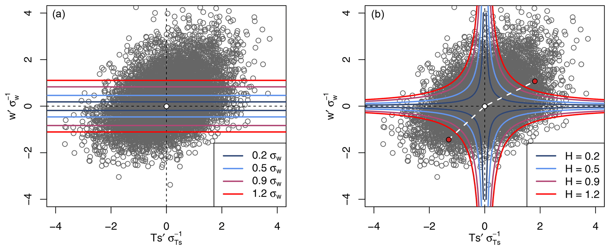
Figure 1Schematic quadrant plots to visualize the application of linear (a) and hyperbolic (b) deadbands. Different colored lines show which data points are included for different deadband sizes. The white dot marks the origin in both panels. In the (b), solid red dots mark the mean and mean for up- and downdrafts when a hyperbolic deadband with H=1.2 is applied (red). The dashed white lines in (b) connect the red dots with the coordinate system origin. The deviation from 180∘ of the angle spanned between these lines is a measure for the asymmetry of the sample distribution.
When applying a linear deadband to w′ (Fig. 1a), no sample is taken if the magnitude of w′ is below a certain threshold. This threshold can be held constant or adjusted dynamically in time. Dynamical adjustments are often done by scaling with the standard deviation of the vertical wind σw. The linear deadband appears as two horizontal lines in the quadrant plot in Fig. 1b, defined by the linear equation
where a is a constant.
This approach offers the advantage of the deadband being proportional to the integral strength of the turbulent diffusive process transporting the trace gas of interest. During field sampling, the size of the deadband is dynamically adjusted by applying a back-looking running time window of fixed length to compute a⋅σw. Baker (2000) recommends a linear deadband with a width of a=0.9 to obtain the best estimate of the slope m in the βw approach.
Hyperbolic deadbands are specifically designed to exclude eddies with little flux contribution and maximize the concentration difference between the two sampling reservoirs. The exclusion of up- or downdrafts is in this case not only based on vertical wind velocity but also on the fluctuations of a proxy scalar. Hyperbolic deadbands are defined by the dimensionless factor H (“hole size”), which is defined as in Bowling et al. (1999):
Plotting such a defined function in velocity–scalar space demonstrates that an area in the shape of two hyperbolas is excluded (Fig. 1b). The REA method using a hyperbolic deadband is often referred to as the hyperbolic REA (HREA) technique. Here, we only consider symmetrical deadbands, presuming symmetrically distributed flow and concentration statistics. Effects of non-Gaussian distributed w′ and p′ can be gleaned from investigating higher central statistical moments.
The use of large deadbands must be done with caution because they exclude a significant fraction of the data from being sampled. As a result, the random sampling error, which is related to , can be increased due to the decreased sample size n. In addition, the time period between opening and closing a sampling valve is reduced for large deadbands, which may introduce additional errors because of the increased difficulty of sampling short-lived events precisely. An estimate for random error can be derived from the asymmetry of the sample distribution. Considering the quadrant plot of the data points sampled in one averaging period, the distribution can be represented by two points: (), () and (), (). Considering the example in Fig. 1b, these points are drawn for the largest deadband size (red dots). Ideally, these two points fall into a unique linear relationship intersecting the coordinate system's origin (white dot). However, the use of large deadbands can introduce large asymmetry between up- and downdrafts. The asymmetry is shown as a dashed white line in Fig. 1b, containing a bend. This bend, which can be expressed as an angle different from 180∘, is one measure for the asymmetry of the sample distribution.
2.5 Selected models and evaluation metrics
In this study, we compare β and deadband approaches used in the literature and evaluate their performance for the prediction of the latent heat flux over different terrestrial surfaces. The following four REA methods have been chosen for the analysis.
-
Model 1. βT (Eq. 2) uses the sensible heat as proxy and a dynamically adjusted linear deadband scaled with σw (Eq. 9).
-
Model 2. βT (Eq. 2) uses the sensible heat as proxy and a dynamically adjusted hyperbolic deadband scaled with σw (Eq. 10).
-
Model 3. βw (Eq. 7) uses a dynamically adjusted linear deadband scaled with σw (Eq. 9).
-
Model 4. βT, const (Eq. 8; median over the complete field experiments) uses sensible heat as a proxy and a dynamically adjusted linear deadband scaled with σw (Eq. 9).
For each of the models, four different deadband widths are examined both for linear (0.2, 0.5, 0.9, and 1.2σw) and hyperbolic (H=0.2, H=0.5, H=0.9, and H=1.2) deadbands. One simulation was run as a control with a null deadband. To dynamically adjust deadband size, back-looking windows of 60 and 300 s duration were tested. The comparison of these two window sizes yielded only negligible differences between the computed fluxes for the three data sets; hence we chose to present results from the 300 s window only.
In the next steps, we proceed as follows: each of the above models is first optimized with respect to the deadband size. To do so, the accuracy of each β model is assessed by comparing the median ratio of the modeled flux, FREA, and the corresponding direct EC-measured flux, FEC, : If this ratio is greater than 1, then the flux is overestimated by the model, and if it is <1, the flux is underpredicted. In addition, the variability in this ratio is inferred using the root mean square error (RMSE), which provides a measure of the precision of each model. It is computed using the difference between the modeled REA flux and the measured EC flux.
The deadband width, which is found to yield the most accurate water vapor flux (taking into account relative error and RMSE) is then further evaluated. Table 2 summarizes the different model setups tested, along with the optimal deadband sizes.
3.1 Site descriptions
We selected three sites with strongly contrasting vegetation cover and surface roughness, vegetation architecture, and biogeochemical processes governing the vertical exchange of CO2, water vapor, and sensible heat to test the different β models (Table 1). Using sites with stark differences provides robust recommendations for REA users choosing an optimal β for their site.
Panofsky (1984)Table 1Description of the three data sets used in this study: numbers from quality-screened data, aggregated to 30 min temporal resolution. IQR signifies interquartile range.
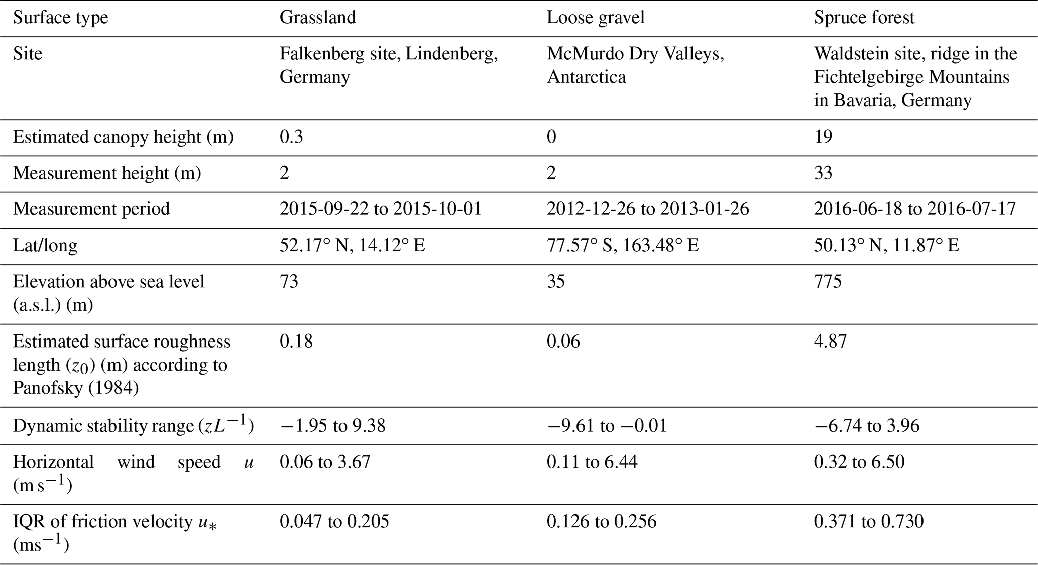
The grassland data (Thomas et al., 2021) were collected in Falkenberg, Germany at the German Meteorological Service (Meteorological Observatory Lindenberg; see Table 1 for details). The central part of the field site is a flat meadow of dimensions 150 × 250 m covered by short grass (vegetation height <20 cm). This area is surrounded by grassland and agricultural fields in the immediate vicinity, a small village is situated about 600 m to the southeast, and a small but heterogeneous forest area lies to the west and northwest at about 1 to 1.5 km distance. Within the flux footprint of the tower, the main vegetation cover consisted of grassland and recently harvested maize. The soil type distribution in the area around Lindenberg is dominated by sandy soils covered by a layer of loam, which is typically found at a depth of between 50 and 80 cm. Lindenberg represents moderate mid-latitude climate conditions at the transition between marine and continental influences. Monthly mean temperatures (1961–1990) vary between 1.2∘C (January) and 17.9∘C (July), and the mean annual precipitation sum is 563 mm (Beyrich et al., 2002; Neisser et al., 2002). In contrast, the McMurdo Dry Valleys (Thomas and Levy, 2021) span 4800 km2 of ice-free land in Antarctica and are covered by rocks and glacial till (Linhardt et al., 2019). The area ranges from sea level to 2000 m in elevation and is composed of ice-covered lakes, short-lived streams, and rocky ice cemented soils that are surrounded by glaciers. The mean annual temperature in the Dry Valleys ranges between −17 and −20∘C. The low precipitation relative to potential evaporation, low surface albedo, and dry katabatic winds descending from the Polar Plateau result in extremely arid conditions (Clow et al., 1998).
Finally, we use a data set acquired at a spruce forest site in the German Fichtelgebirge (Thomas and Babel, 2021) that spans ca. 1000 km2 of northeastern Bavaria, Germany. Its summits reach 1053 m a.s.l. (above sea level; Schneeberg) and 1023 m a.s.l. (Ochsenkopf). The Waldstein hillsides comprise a mountainous ridge reaching up to 877 m a.s.l. (Gerstberger et al., 2004). The measurement site is located at about 800 m a.s.l. The prevailing tree species at the Waldstein site is Norway spruce (Picea abies, L.) with a mean canopy height of 19 m. The EC flux instrumentation (2 m high) was installed on top of a 31 m high scaffolding tower reaching above the highest tree tops, resulting in a total measurement height of 33 m above ground. Monthly mean temperatures (1961–1990) vary between −4.2∘C (January) and 14.1∘C (July), and the mean annual precipitation sum is 1156 mm (Foken, 2003).
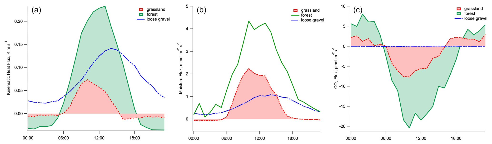
Figure 2Ensemble-averaged diurnal fluxes of kinematic heat flux (a), moisture flux (b), and CO2 flux (c) at each of the three sites. The traces where the sign of the flux changes are filled to the zero line for clarity.
The comparison of the kinematic heat, moisture, and CO2 fluxes in the three ecosystems highlights the diverse exchange behavior trace gases can exhibit depending on the environments (Fig. 2): the differences in albedo and length of daylight are reflected in the variation in the sensible heat fluxes. The heat flux at the loose-gravel-covered site in the Dry Valleys of Antarctica particularly stands out due to the perpetual sunlight experienced during the campaign period. A diel course is still observed, but the flux is constantly directed away from the surface, as indicated by the positive values. The diel patterns visible at both the forest and the grassland site are similar, showing positive sensible heat flux during daytime and negative at nighttime. The difference in flux magnitude between forest and grassland can be attributed to the distinct differences in vegetative canopy properties. The tall dark canopy with low surface albedo is considerably different from the shorter and more reflective grassland canopy. The range in latent heat and CO2 fluxes displays the impact of the vegetation. The loose-gravel site, which is the most extreme site void of vegetation, shows a net exchange of CO2 equal or close to zero between the surface and the atmosphere, whereas both forest and grassland sites display an expected pattern of dominant CO2 uptake during the daytime and respiration during the nighttime. The larger leaf area index in the forest of around 5 m2 m−2, compared to 3 m2 m−2 for typical grassland areas, like in Lindenberg, causes a greater magnitude of latent heat flux because of the transpiration and concurrent greater exchange of CO2.
3.2 Instrumentation and post-field data processing
The turbulence observations consisted of the three-dimensional wind vector and sonic temperature collected by a sonic anemometer (Lindenberg: CSAT3, Campbell Scientific Ltd., Logan, UT, USA; Dry Valleys: 81000 VRE, R.M. Young Company, Traverse City, Michigan, USA; Waldstein forest: USA 1-FHN, Metek, Elmshorn, Germany) and water vapor and carbon dioxide molar densities measured by an open path analyzer (LI-7500, LI-COR Inc., Lincoln, NE, USA) both recorded by a data logger (CR3000, Campbell Scientific Ltd., Logan, UT, USA). The sampling rate was 20 Hz. Spikes and outliers in raw turbulence time series were discarded according to Vickers and Mahrt (1997) with an initial 5σ criterion. Resulting gaps in the high-frequency time series were linearly interpolated. Covariances were maximized by shifting the scalar time series relative to that of the vertical velocity by a dynamically determined lag. This means that, for each sampling period, the scalar time series were shifted to achieve maximum cross-correlation with the vertical wind time series (Foken, 2008). For the Reynolds decomposition, a perturbation and averaging timescale of 300 s was chosen. Using this shorter than the common 30 min timescale is motivated by the intention to filter out the effects of longer-lived motions, as described in Vickers et al. (2009).
Raw velocities were rotated using the first two steps in the common three-dimensional rotation method ensuring that the mean crosswind and vertical wind components equal zero. A spectral correction was applied to EC fluxes following Moore (1986) to account for flux losses resulting from the sensor design and data collection. Quality assurance and quality control flags were applied to the computed REA and EC fluxes by testing for stationarity and developed turbulence following Foken et al. (2004). All data with flags >1 were discarded from subsequent analysis. Since the flags do not capture all unphysical flux estimates, additional hard thresholding was applied. To minimize the substantial random error in turbulent flux estimates over short averaging intervals, six subsequent 300 s intervals were block-averaged to yield one 30 min flux estimate for both the REA and EC methods following Vickers et al. (2009).
Since simulating REA sampling requires selecting individual high-frequency data from a continuous time series and computing density-corrected scalar higher-order moments, an ad hoc density correction was applied to the water vapor and carbon dioxide molar densities (Detto and Katul, 2007) prior to flux computations. To this end, molar densities were multiplied by the ratio of the instantaneous mean density of dry air . This correction removes the density fluctuations due to changes in external conditions. EC fluxes were computed using the common post hoc density correction (Webb et al., 1980). Even though open-path observations in cold environments such as the McMurdo Dry Valleys suffer from sensor heating artifacts not captured by either our ad hoc or the common post hoc Webb, Pearman, and Leuning (WPL) correction (Burba et al., 2008), we decided to not apply this additional correction in this study since we are interested in the relative flux error only. Instead, we applied a constant offset of 0.35 µmol m−2 s−1 to the CO2 flux densities to force them through zero for illustrative purposes. This choice has no effect on the study results.
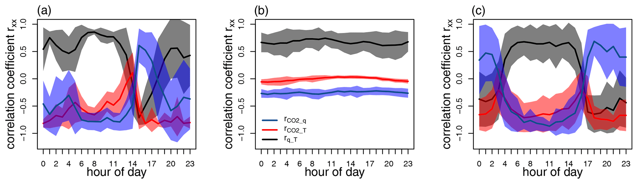
Figure 3Diurnal course of scalar–scalar correlation coefficients rsp at the meadow site (a), the loose-gravel-covered Dry Valleys site (b), and the Waldstein forest site (c); ± 1 standard deviation σ is drawn as a semi-transparent area around the mean curves of rsp.
For the REA flux estimation, hyperbolic and linear deadbands of varying sizes were tested. The linear deadband size was scaled by increasing fractions of σw computed over a back-looking running window of length 300 s (e.g., Ren et al., 2011; Arnts et al., 2013; Movarek et al., 2014). It must be noted that the deadbands are applied only to the statistics to compute and (see Eq. 6). In contrast, the entire population of vertical velocities observed in an averaging period were used to compute . Applying the deadbands for computing also the vertical velocity variance leads to significant flux overestimation since σw increases with increasing deadband size. In the final step, the same thresholds for physical plausibility which were applied to the computed EC fluxes were also used to remove unplausible REA flux estimates from the data sets. These thresholds were chosen individually for each scalar and each data set due to the wide range of meteorological and biochemical conditions covered in this study.
This study evaluates estimates of the latent heat flux obtained using different REA techniques. The approaches requiring a proxy scalar rely on the sensible heat flux , which is a common choice since it can be measured with a higher precision compared to, for example, CO2 in certain low-flux conditions.
We structured this section as follows. First, scalar correlation coefficients for the different ecosystems are presented in Sect. 4.1. In Sect. 4.2, we describe the choice of an optimal deadband size for each REA model based on both and the RMSE. The optimized REA models are then evaluated in Sect. 4.3 with respect to the effects of the diurnal course and atmospheric stability. To test the applicability of our findings to other scalars, we are including an evaluation of simulated CO2 REA fluxes for all four models, using Ts as proxy for models 1 and 2, in Appendix A. Here, the same deadband sizes are used, which were previously chosen as the optimum for the water vapor flux in Sect. 4.2 .
4.1 Scalar similarity across land surfaces
Scalar similarity is an important assumption for the βT models (models 1 and 2) and can be used as one evaluation metric for the method.
To assess whether a scalar can serve as a viable proxy p for the trace gas of interest s, the similarity in source and sink strength of two can be represented by their correlation coefficient rsp (Eq. 3). We first analyze the temporal dynamics of scalar similarity across the different land surfaces: the diurnal courses of the correlation coefficients of and , and , and and , ensemble-averaged over the complete field campaigns, are presented in Fig. 3. Pronounced temporal changes in scalar similarity within the diurnal cycle at the grassland and forest sites are in strong contrast to the constant values observed for all analyzed rsp in the Dry Valleys. The patterns can be explained by the influence of radiative forcing, which governs both the physical heat exchanges and biological photosynthesis and evapotranspiration, highlighting the constant daylight observed during the measurement period in the Dry Valleys. All three correlation coefficients change sign at the grassland site around 14:00 local time, associated with the expected change in dynamic stability resulting from the change in the direction of the sensible heat flux. A similar diurnal pattern is observed in the forest site; however, the change in sign of the correlation coefficient happens approximately 2 h later in the day. In contrast, the correlation between and is positive throughout the nocturnal period in the forest site and negatively correlated in the grassland site, where regular dew formation occurs (which can be also observed in Fig. 2). The scalars tend to be poorly correlated at nighttime compared to daytime as a result of weak turbulence and associated diminished scalar transport efficiency for both sites.
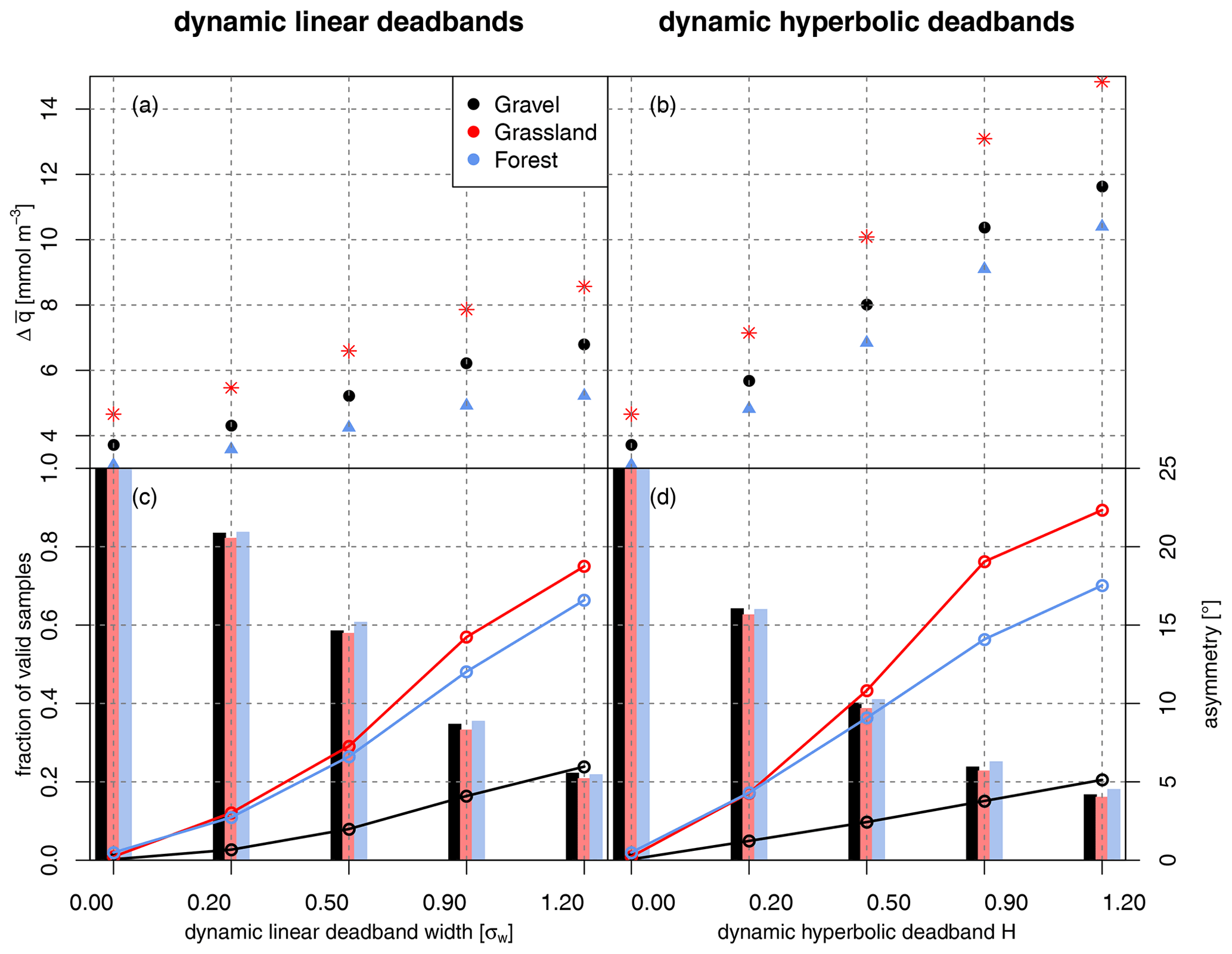
Figure 4Effect of deadband size on the concentration difference and measures of the random error. Panels (a) and (b) show the concentration difference between up- and downdraft reservoir as a function of deadband size (linear deadbands in panel a and hyperbolic deadbands in panel b). (c, d) The bars show the fraction of samples used for flux computation, and the overdrawn circles show the asymmetry between up- and downdraft vectors in the quadrant plot. The asymmetry is calculated as the absolute deviation in the angle between a straight line and a bent line constructed using the center points of up- and downdrafts and the origin in the quadrant plots. See Fig. 1 and accompanying text for details.
4.2 Determining the optimal deadband size for each of the β methods
Figure 4 summarizes the effects of deadband size on the water vapor concentration difference between up- and downdraft reservoirs and the fraction of samples used for flux computation, along with the asymmetry measure introduced in Sect. 2.4. As expected, increases with increasing deadband size for both linear and hyperbolic deadbands at all three sites. This increase is more pronounced for hyperbolic deadbands compared to the linear deadbands (Fig. 4a and b). The hyperbolic deadbands have the desired effect of maximizing the concentration difference between the two sampling reservoirs. For H=1.2, almost a factor of 3 increase in water vapor concentration difference between updraft and downdraft sampling reservoirs can be achieved. The HREA technique therefore has the potential to provide concentration differences detectable by instrumentation with high detection limits or when measuring chemical species with very low mixing ratios. However, as mentioned above, large deadbands can introduce a large random error because they exclude a large portion of the sample data points. The decrease in sample size with increasing deadband size is similar across all three sites (Fig. 4c and d) and should be considered when choosing an optimal deadband. For example, for a hyperbolic deadband with H=0.2, approximately 40 % of the sampling period is excluded, which results in an increased asymmetry (Fig. 4d). This effect is more pronounced for the forest and meadow surfaces than for the gravel site, possibly caused by a larger heterogeneity in scalar sink and source distribution.
In the next step, we evaluate each REA model individually and select an optimal deadband size with respect to selected uncertainty metrics of the β model: we chose to include measures of the precision and the accuracy of the methods by comparing and RMSE for the simulated deadbands. The ratio and RMSE obtained for different linear deadband widths using the βT model (model 1) are shown in Fig. 5. Results strongly vary across the different ecosystem types: while the REA water vapor flux at the Antarctic gravel site is very similar to that obtained from the EC technique, as indicated by negligible RMSEs, the estimates obtained at the forest and meadow sites feature a much larger RMSE. This difference can be explained by the differences in the degree of scalar–scalar similarity between the latent and sensible heat fluxes of the purely physically driven site as opposed to the biologically active sites. The scalar fluxes are modulated by a varying degree of vegetation responses adding to the complexity of the scalar–scalar correlation rq,T and diurnal changes in sign (Fig. 3). The use of no deadband (deadband width = 0) leads to an overall small underestimation of the EC fluxes (4 % to 8 %) across all sites. This underestimation is reduced with the use of a deadband at the gravel site; however, the systematic bias is not resolved by applying a deadband at the other two sites, but in contrast it increases this underestimation. Such a systematic bias could in theory be corrected for in post-processing, but the magnitude of the correction would have to be determined for each site defying our intention of providing general recommendations. This flux bias varies more between sites than with deadband width; therefore, this correction method should only be applied if the user knows the transport characteristics and scalar sink and source distribution well. Based on the flux bias and RMSE, a linear deadband with 0.5σw width is chosen as the optimized deadband size for further comparisons with the linear βT approach.
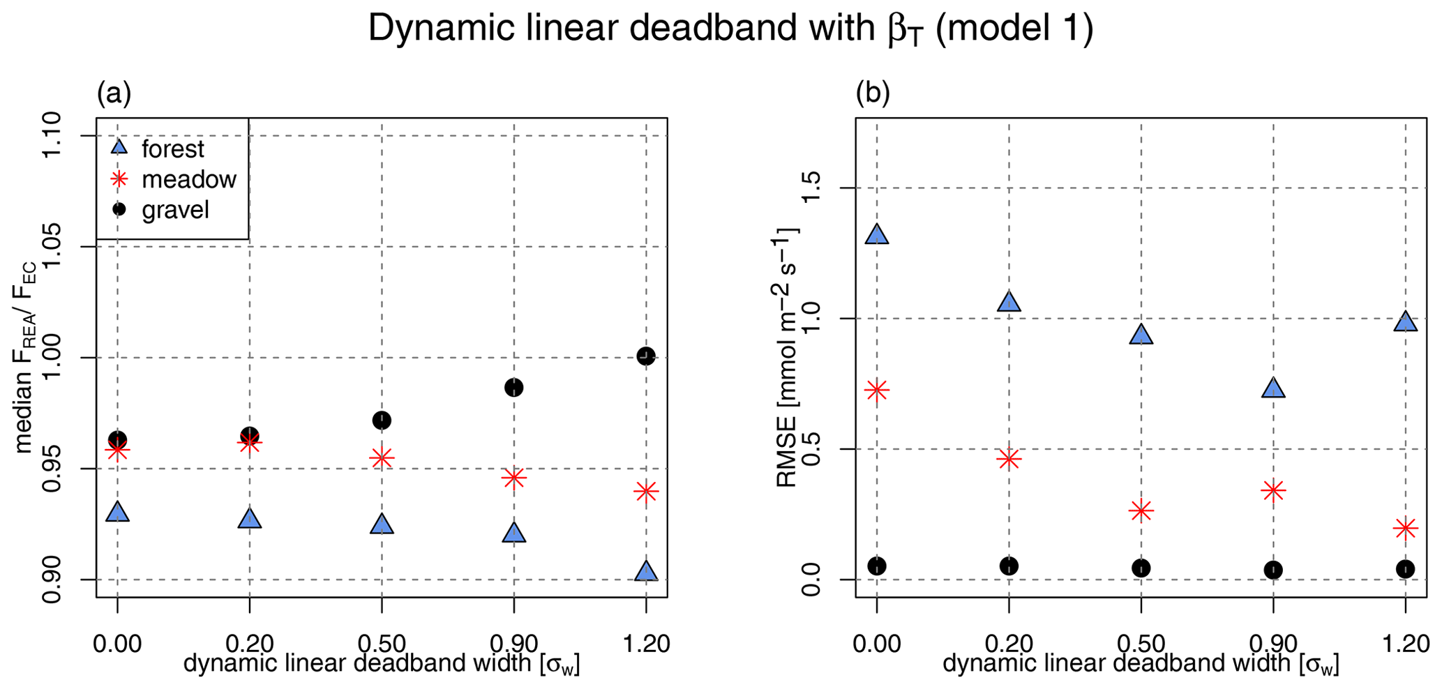
Figure 5Errors as a function of dynamic linear deadband width. The x axis is the scaling factor a multiplied by the vertical wind standard deviation σw in Eq. (9) to define the deadband threshold. (a) Median (latent heat flux simulated with sensible heat as a proxy) ratio for each of the simulated dynamic deadband widths; (b) RMSE for each of the simulated dynamic deadband widths.
The results for the βT model using a hyperbolic deadband (model 2) are shown in Fig. 6. Both median FREA/FEC and RMSE are of the same order of magnitude compared to the linear deadband approach for βT (Fig. 5, model 1). However, the hyperbolic deadband offers an increase in concentration difference that is considerably larger in comparison, which led to its use in several studies (e.g., Held et al., 2008; Movarek et al., 2014).
Interestingly, the observed underestimation of the latent heat flux is lessened for the forest and gravel sites when hyperbolic deadbands are applied, whereas it becomes larger for the meadow site. For the gravel site, the bias even changes sign for large hyperbolic deadbands. The RMSE shows no significant improvement when the small-scale eddies with small flux contributions are excluded irrespective of ecosystem. Based on Fig. 6, a hyperbolic deadband of H=0.5 is chosen for further analysis as it offers an increase in by 100 % (Fig. 4).
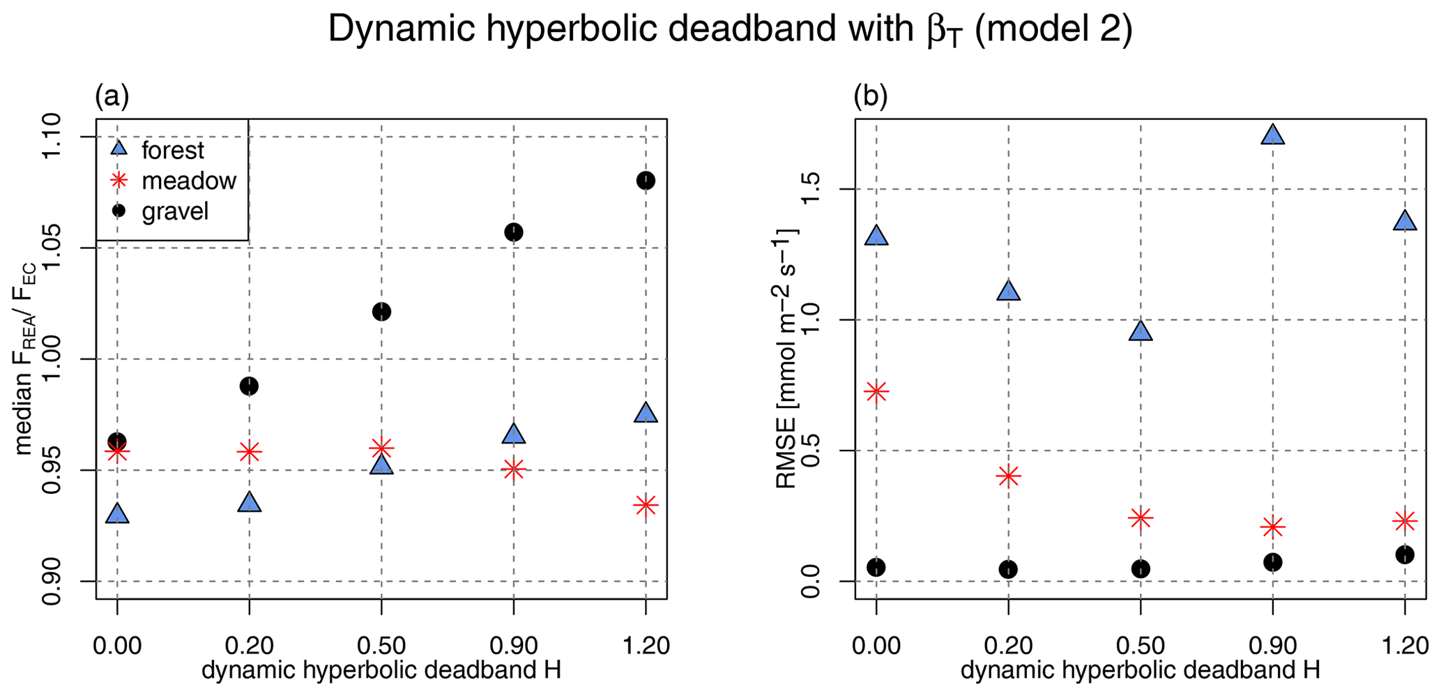
Figure 6Errors as a function of dynamic hyperbolic deadband size. The x axis is the H parameter in Eq. (10), which defines the deadband size. (a) Median (latent heat flux simulated with sensible heat as a proxy) ratio for each of the simulated dynamic deadband sizes; (b) RMSE for each of the simulated dynamic deadband sizes.
When applying a linear deadband to model 3 using βw derived from the wind statistics alone, a positive flux bias (5 %–10 %) becomes evident when no deadband is applied (Fig. 7). This observation confirms the findings of Katul et al. (1996): eddies characterized by a large vertical perturbation (w′) are known to contain smaller perturbations in sensible heat () than predicted by the linear fit of and , whose slope is dominated by the many small-scale eddies characterized by a greater . The use of deadbands puts more weight on large eddies; thus deadbands are convenient to improve the estimate of the w′ vs. , resulting in a smaller slope m for this model. The choice of deadband size has clear implications for how well the βw model performs. The RMSE for this method is significantly smaller than the values observed in the two βT models. Overall, the pattern in relative and absolute error is more consistent for the βw model across the three ecosystems compared to the βT models. The optimal deadband width 0.9σw, which was proposed by Baker (2000), provides low systematic bias, high precision, and the minimum in RMSE for all sites in Fig. 7. However, the use of this deadband size excludes more than 60 % of the available data (see Fig. 4), so we chose a linear deadband width of 0.5σw instead. This choice yields a similarly high accuracy and precision and therefore was our optimal choice for model comparisons.
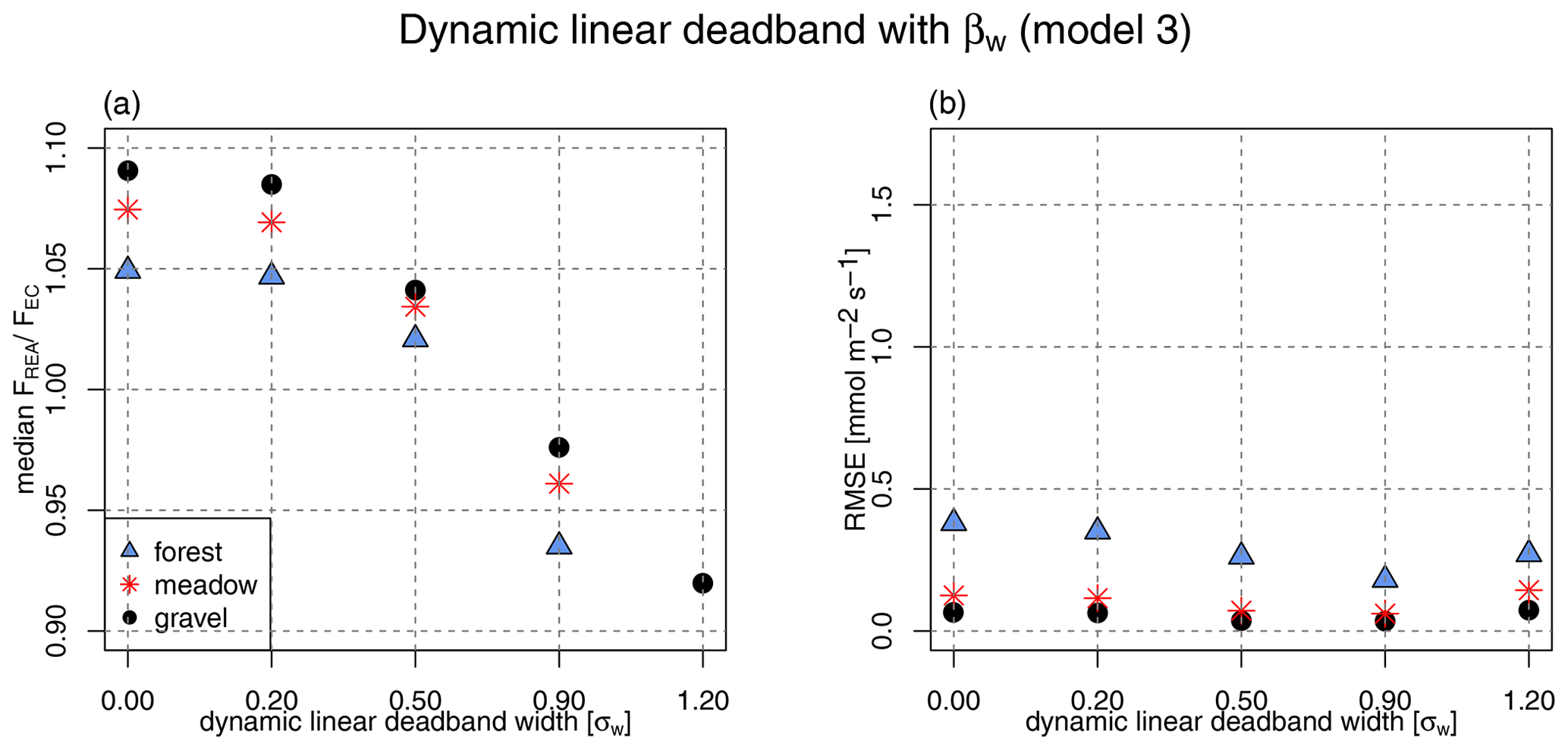
Figure 7Errors as a function of dynamic linear deadband width. The x axis is the scaling factor a multiplied by the vertical wind standard deviation σw in Eq. (9) to define the deadband threshold. (a) Median FREA/FEC ratio (latent heat flux simulated using the REA approach described in Baker, 2000) for each of the simulated dynamic deadband widths; (b) RMSE for each of the simulated dynamic deadband widths.
The performance of the constant βT, const (model 4) is illustrated in Fig. 8, in which the FREA/FEC and RMSE was calculated using a constant β and dynamic linear deadbands of different sizes. FREA/FEC is close to 1 for all deadband sizes in this model. The RMSE is, similarly to that of the βw (model 3, Fig. 7), constantly low for all ecosystems. Following Grönholm et al. (2008), we chose a deadband size of 0.5σw for further comparison.
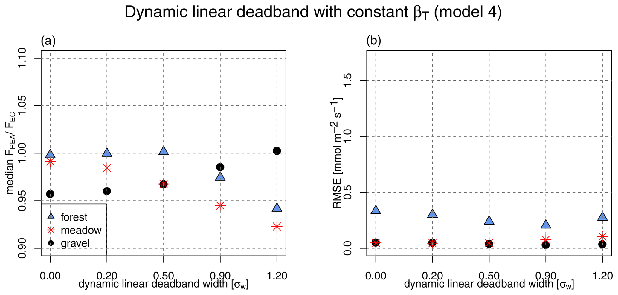
Figure 8Errors as a function of dynamic linear deadband width. The x axis is the scaling factor a multiplied by the vertical wind standard deviation σw in Eq. (9) to define the deadband threshold. (a) Median FREA FEC ratio (latent heat flux simulated using constant βT, const and dynamic linear vertical wind deadband) for each of the simulated dynamic deadband widths; (b) RMSE for each of the simulated dynamic deadband widths.
Table 2 summarizes the chosen optimum deadband widths for each of the four methods and gives the medians of the respective β parameters for each of the three sites. The values for model 1 and model 4 are equivalent because the medians over the whole considered period are shown, which results in the definition of model 4.
Table 2Median β parameters for the chosen optimum deadband sizes for each of the four models and each of the three sites.

4.3 Evaluation of optimized β models
After choosing an optimal deadband size for each REA model, we now proceed to analyzing the effects of the diurnal light variability and atmospheric stability on flux estimates.

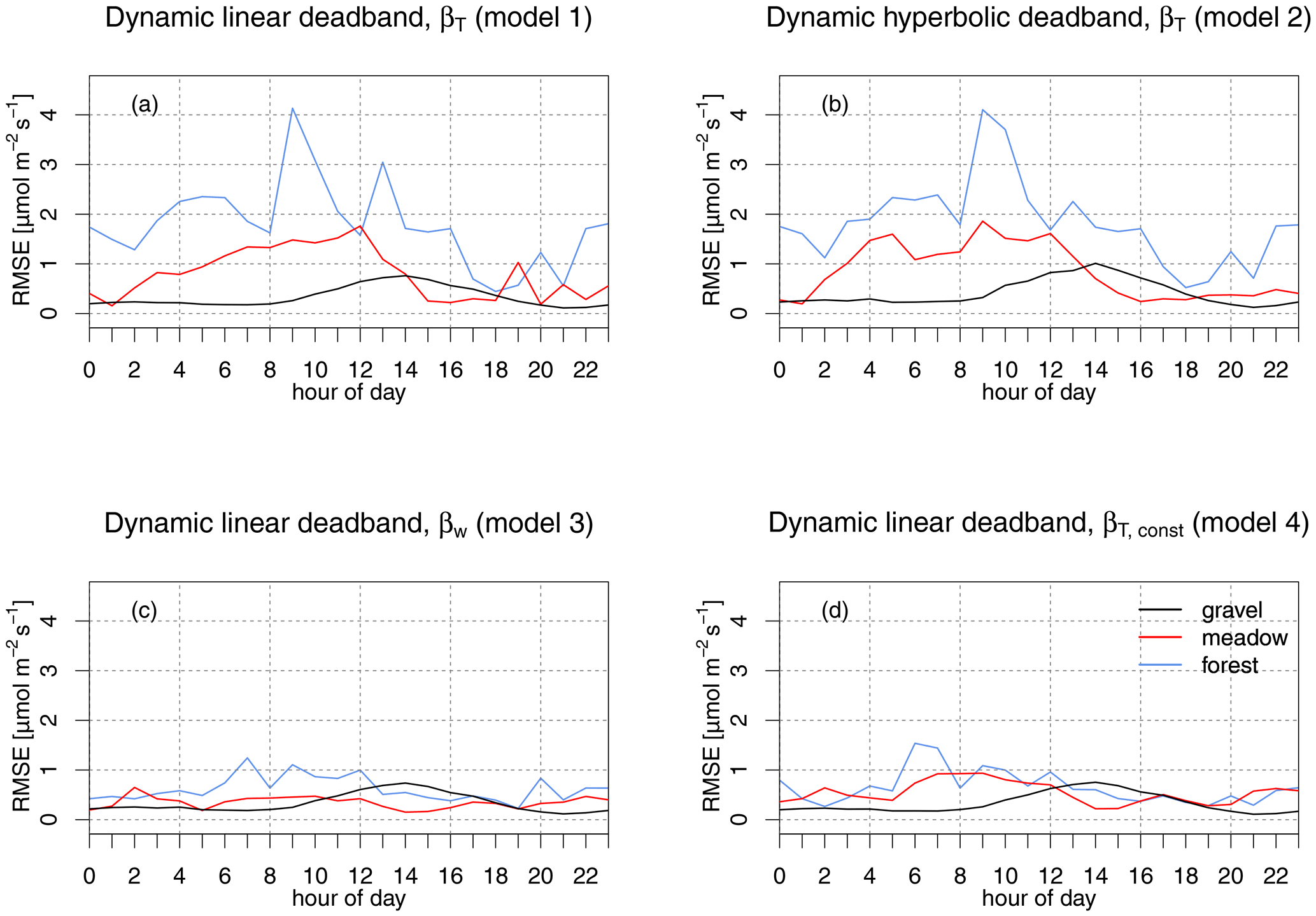
Figure 9Flux RMSE as a function of the hour of day (local time) for each of the optimized β models. Panel (a) shows the RMSE of the proxy-based model using a dynamically adjusted linear deadband (model 1), scaled with 0.5σw. In this panel, there is one extreme value with RMSE > 3, which is outside of the plot boundaries. Panel (b) shows the proxy-based model using a dynamically adjusted hyperbolic deadband (model 2) with H=0.5. Panels (c) and (d) show the RMSE of the βw REA model (model 3) and the constant βT, const approach (model 4), respectively, both with a dynamically adjusted linear deadband of width 0.5σw.
4.3.1 Effect of the diurnal course
Data were binned according to the hour of day, and the RMSE was computed for each hour. Each panel in Fig. 9 shows the result for the different models 1–4 at the optimal deadband size. All four REA models successfully capture the flux at the loose gravel site; however, discrepancies between FREA and FEC become obvious for the meadow and forest sites. Here, the RMSE for model 1 and model 2 (Fig. 9a and b) is significantly larger compared to the REA methods applied by models 3 and 4 (Fig. 9c and d). The constant βT, const (model 4) and the βw method (model 3), both utilizing a dynamic linear deadband, feature a negligible RMSE for the gravel and the meadow sites, as well as a small RMSE below unity for the forest site. The βT models have a distinct peak in RMSE at the meadow site around 14:00 local time, which coincides with a low scalar–scalar correlation of water vapor and heat (Fig. 3). At the forest site, the uncertainty in FREA is large throughout the diurnal course for both βT models due to the large variability in rq,T. During times of strong variability, the difference FREA−FEC can be of the same order of magnitude as the absolute evapotranspiration. This occasional poor performance of the βT model does not change significantly across the range of tested linear and hyperbolic deadbands. Filtering out small-scale eddies therefore does not improve flux estimates. However, hyperbolic deadbands still increase the concentration difference if the detection limit is of concern. Applying models 1 or 2 for observing the diurnal variation in the exchange of a trace gas must be done carefully when choosing a proxy that exhibits a pronounced diurnal cycle. The key assumption in these approaches is that the proxy and trace gas of interest have similar temporal or spatial dynamics, which introduces large uncertainties if the temporal dynamics of the scalar of interest remain unknown or are not known a priori.
So far, only one proxy–scalar combination was investigated in this study. However, showing that the presented results are also valid for other scalars is critical for their applicability. The data sets allow for including CO2 for additional validation. The CO2 flux was simulated with the optimized models 1–4 (using the deadband sizes summarized in Table 2), with sensible heat as the proxy for models 1, 2, and 4. The comparison of ratio and RMSE indicated that the optimum deadband sizes found for H2O (Table 2) are also valid for CO2. The hourly RMSEs are included in Appendix A in Fig. A1. A similar pattern in the diurnal RMSE as observed for the H2O flux also emerges for CO2: models 1 and 2 both yield higher RMSEs than models 3 and 4, the forest site exhibiting larger RMSEs than the meadow site. These findings suggest that the results presented here for the H2O flux are also valid for the CO2 flux and possibly other atmospheric compounds. However, we cannot arrive at a final conclusion for other (including reactive) scalars, for which REA is often applied since fast-response analyzers are missing. Answering this question is beyond the scope of this study and should be considered in future research.
4.3.2 Effect of atmospheric stability
The observed relationship between the βT model bias and changes in scalar–scalar similarity suggests a dependence from shortwave radiative forcing leading to changes in atmospheric dynamic stability. A dependence of the βT factor on atmospheric stability has been shown in previous studies. Here, we extend this analysis to the effects of deadband type and size in addition to the βw method. For comparison reasons, we evaluate the dependence of the β on dynamic stability () similar to Ammann and Meixner (2002) (their Fig. 3), who first documented a relationship between βT and atmospheric stability. Figure 10 shows the models for time-varying β binned into logarithmically spaced classes of dynamic stability. These classes were defined such that the range of dynamic stability spanned by each bin is equally sized in the logarithmic space. For the two dynamic proxy models (models 1 and 2; Fig. 10a and b), βT without deadband approximately follows the relationship found by Ammann and Meixner (2002), i.e., a constant βT for unstable conditions, and an increase from neutral and stable conditions of . However, this increase is associated with large statistical uncertainty and only due to the data from the forest site (please note that Fig. 10 combines the observations from all three sites). We therefore recommend exercising caution when using stability-dependent parameterizations of βT. Variability in βT generally decreases with increasing deadband size. Model 3 (right panel in Fig. 10) shows a very different behavior: βw is apparently unrelated to atmospheric stability and displays a generally lower variability than βT. This finding explains why the results in Figs. 5, 8, and 9 for the βw and constant β applying a dynamic linear deadband are so strikingly similar: βw for the selected optimal deadband width of 0.5σw shows little variability, which makes this approach similar to applying a constant β factor.
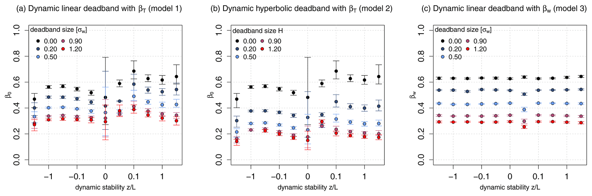
Figure 10Dependence of the βT and βw factors on the atmospheric stability . Data were binned in logarithmic, evenly spaced stability classes. The markers are drawn at the median β of each bin, and the bars mark the interquartile range (IQR). This figure combines valid data points from all three sites.
It was pointed out in previous REA studies that βw scales with the fourth central statistical moment of the vertical velocity perturbations' distribution by altering the w′ vs. c′ relationship. We therefore investigated the impact of the w′ kurtosis on the βw factor for different linear deadband sizes. Katul et al. (2018) found that two different factors, which both depend on , contribute to βw and whose impacts can cancel out if their magnitudes are similar. The first effect, leading to an decrease in βw with increasing (positive) , depends on the excess kurtosis or flatness factor of the w′ distribution. The second effect, resulting in an increase in βw with increasing , is a result of the transport efficiency eT (Wyngaard and Moeng, 1992), as well as source strength and asymmetry in the w′ distribution. The superimposition of these two processes could be an explanation of why there is no clear dependence of βw on dynamic stability visible in Fig. 10.
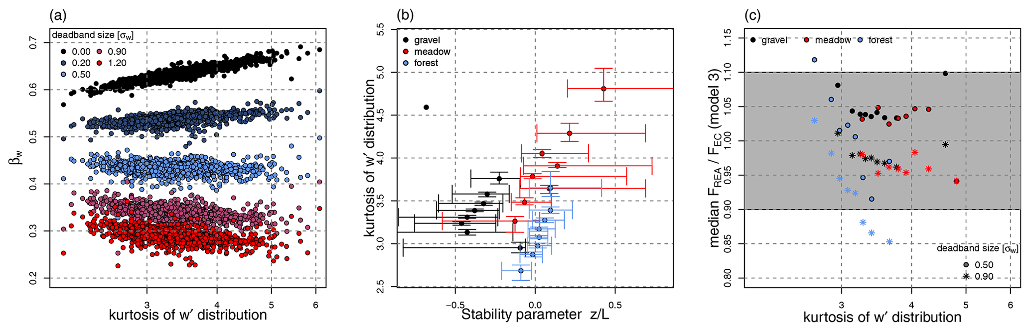
Figure 11This figure only presents results from REA model 3 (βw). (a) βw as a function of w′ kurtosis for different deadband widths (not binned). Valid data points from all three sites are combined in this panel. (b) The stability parameter as a function of the w′ kurtosis. Data were binned into eight kurtosis bins with an equivalent number of data points. Only bin medians are displayed, and bars mark the IQR. (c) Median FREA by FEC as a function of w′ kurtosis for the optimal deadband widths, 0.9σw and 0.5σw, which were determined by Baker (2000) and in this study. Data were grouped into the same kurtosis bins as in (b). The grey area marks the ±10 % range, which is the error assumed in EC applications.
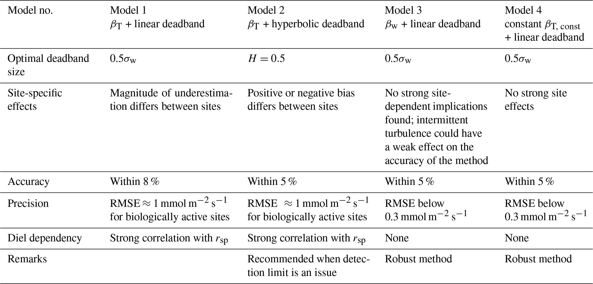
Table 3Summary of the REA models compared in this study, along with main findings.
The relationship between the w′ distribution's kurtosis and the βw factor is illustrated in Fig. 11: consistent with Katul et al. (1996, 2018) the βw factor without deadband increases as a function of w′ kurtosis (Fig. 11a). The plot collapses data from all three ecosystems into a single linear relationship. This finding suggests that the turbulence statistics, including the βw factor, are site-independent despite the significant differences in climate and surface characteristics across the three ecosystems (canopy height, roughness, etc.). This is confirmed by the nearly identical average βw values found for the three sites in Table 2 of 0.43–0.44. In connection with the small spread of βw values in Fig. 11 and the strikingly similar RMSE for models 3 and 4 (Fig. 9), our results suggest that βw can be considered a both site- and time-independent constant.
Kurtosis is in turn expected to be related to dynamic stability when changes in turbulence statistics and diabatic conditions lead to a non-Gaussian distribution of w′. As a result, the kurtosis of the w′ distribution becomes different from 3, which is the value for a Gaussian distribution. In Fig. 11b, w′ kurtosis is plotted against the stability parameter . Figure 11c displays the resulting median as a function of w′ kurtosis. Only the model results for REA applying a linear deadband with widths of 0.5 and 0.9σw are displayed here for improved visibility. While no clear trend is observed at the grassland site and only a slightly negative trend is visible for the gravel site, we can detect a strong decrease in the median as a function of w′ kurtosis for the forest site. However, as indicated by the shaded area in Fig. 11c, most points lie within the boundaries of ±10 %. Only the bins with the highest and lowest kurtosis classes at the forest site are outside of this range. These error bounds are of the magnitude as the error assumed in EC applications. We suspect that the large excursions from Gaussian statistics for the forest site are caused by coherent structures forcing cross-canopy vertical exchange, which are a dominant flow mode in the forest flows documented for this site (Thomas and Foken, 2007a, b).
At first sight, it is puzzling why the βw model without deadband (deadband size 0.00) in Fig. 11 shows a considerable variation with the kurtosis, which in turn is related to stability, but basically no dependence of the βw factor on stability can be seen in Fig. 10. This effect is due to the binning: the values in Fig. 10b are bin medians of the kurtosis, while in Fig. 10a, the unbinned 30 min data are shown. Comparing the ranges of the w′ kurtosis in these panels, it becomes apparent that the range between 3 and 4 (Fig. 10b) is much smaller compared to the range between 2 and 5 displayed in Fig. 10a. Within the approximate bounds of 3 and 4 (where most of the data are for all three sites), the βw for zero deadband also has a much smaller systematic variability. Combining these insights with Fig. 10, it means that the bin median value of the w′ kurtosis exaggerates the stability dependence since the within-bin variability is very large, leading to its effect disappearing in the effective βw (Fig. 10c) and FREA FEC (Fig 11c) results. Our findings indicate that the variation in the βw factor with the turbulence statistics seems to have no significant impact on the flux estimate.
This study has compared the performance of four different conditional sampling models to compute the water vapor flux. The tested REA models included the following methods: two approaches relying on the sensible heat Ts as a proxy, using linear (model 1) and hyperbolic deadbands (model 2), a parameterization of the βw factor first introduced by Baker et al. (1992) (model 3), and an approach using a constant βT factor described in Grönholm et al. (2008) (model 4). Models 3 and 4 both use linear deadbands. All deadbands were adjusted dynamically and simulated using a 300 s back-looking window to determine the standard deviation of the vertical wind σw and, for the hyperbolic deadbands, the standard deviation of the proxy scalar Ts, σT. Table 3 summarizes the REA models investigated, along with the main results of this study.
The dynamic scalar proxy (βT) REA models (model 1 and 2) performed well during conditions when the proxy scalar (Ts) and scalar of interest (water vapor) were strongly correlated, i.e., during periods when sources and sinks were similarly spatially distributed and temporally synchronized. Median ratios over the campaign length were close to unity, indicating a generally high accuracy of these two methods. However, during times of low proxy–scalar correlation, the variability in this ratio, measured by the RMSE, was large. This happened particularly at those times of the day when the direction (sign) of the flux changed. Users are strongly cautioned when using the dynamic proxy-dependent REA techniques; the diurnal dynamics of the proxy scalar and trace gas of interest is of central importance. This is also true for scalars subject to both biological and physical forcings driven by time- and space-variant source–sink distributions. Concerning models 1 and 2, choosing the optimal proxy scalar is critical for the method's success. Hyperbolic deadbands, which also require the use of a proxy scalar, are well suited to maximize the concentration difference between up- and downdraft reservoirs more effectively than linear deadbands. The effects of linear and hyperbolic deadbands on the flux estimates were found to be strongly site-dependent for models 1 and 2, i.e., the two dynamic scalar proxy approaches.
For the βw (model 3) and constant βT, const (model 4) approaches, an optimum deadband size was found at 0.5σw. At this deadband size, the variation in βw over time and between the considered sites became very small, making this method almost equal to applying a constant β factor. This finding suggests that βw is a site-independent constant. Overall, models 3 and 4 yielded flux estimates as accurate as models 1 and 2 and even performed significantly better in terms of RMSE.
The dependence on atmospheric stability conditions was evaluated for each method and deadband size. No universal behavior of any stability-dependent () β model for either site was observed. We therefore cannot recommend its use.
Based on the findings obtained in this study, we attempt to formulate the following general recommendations. We overall recommend using either the βw or βT, const approach (model 3 or model 4) using a linear deadband with 0.5σw width. These two models have been shown to perform robustly and be less sensitive to changes in proxy–scalar similarity than models 1 and 2. For applications for which the detection limit is of concern, we propose using the dynamic proxy-dependent approach in connection with a hyperbolic deadband (model 2). Model 2 yielded very similar results to model 1 with respect to the precision and accuracy measures considered in this study. However, hyperbolic deadbands are better suited to maximize the concentration difference between up- and downdraft reservoirs, which is an advantage when investigating fluxes of compounds with very low atmospheric concentrations. For this application it is advantageous to have a well-known site, including scalar–scalar similarity, if possible.
Figure A1 shows the diurnal course of the RMSE for models 1–4 for the CO2 flux. The same deadband sizes which were found to be optimal for the estimation of the water vapor flux were applied. Both proxy approaches (models 1 and 2; panels a and b) result in higher values of the RMSE than the βw (model 3, panel c) and the constant βT, const (model 4, panel d) methods. The RMSE for the gravel site is included in this figure even though the magnitude of the CO2 flux is close to 0 throughout the daily course, and thus no conclusions should be drawn from its RMSE.
Data sets used are available at Zenodo: https://doi.org/10.5281/zenodo.4764499 (Thomas and Levy, 2021), https://doi.org/10.5281/zenodo.4764493 (Thomas et al., 2021), and https://doi.org/10.5281/zenodo.4764490 (Thomas and Babel, 2021).
CKT led the field experiments and performed the REA flux computations. TV and AH performed the data analysis and visualization. TV, AH, and CKT wrote the manuscript.
The authors declare that they have no conflict of interest.
Publisher’s note: Copernicus Publications remains neutral with regard to jurisdictional claims in published maps and institutional affiliations.
Christoph K. Thomas acknowledges funding from the National Science Foundation Career Award in Physical and Dynamical Meteorology, award AGS 0955444.
We would like to thank the German Meteorological Service (DWD) for granting access to their Falkenberg site at the Lindenberg observatory. We further express our gratitude to Wolfgang Babel and Johannes Olesch for their assistance in collecting the observations at the Lindenberg and Waldstein sites in Germany and Joseph Levy for the opportunity of and assistance in collecting observation in the Dry Valleys of Antarctica. Teresa Vogl would like to thank the R project (R Core Team, 2015), especially the developers of the chron (James and Hornik, 2017), xts (Ryan and Ulrich, 2014), and classInt (Bivand, 2015) packages, for providing free data analysis and visualization tools. We also acknowledge the valuable feedback of two anonymous reviewers on a previous manuscript draft.
This open-access publication was funded by the University of Bayreuth.
This paper was edited by Ivonne Trebs and reviewed by two anonymous referees.
Ammann, C. and Meixner, F. X.: Stability dependence of the relaxed eddy accumulation coefficient for various scalar quantities, J. Geophys. Res., 107, D84071, https://doi.org/10.1029/2001JD000649, 2002. a, b, c
Andreas, E. L., Hill, R. J., Gosz, J. R., Moore, D. I., Otto, W. D., and Sarma, A. D.: Stability Dependence of the Eddy-Accumulation Coefficients for Momentum and Scalars, Bound.-Lay. Meteorol., 86, 409–420, https://doi.org/10.1023/A:1000625502550, 1998. a
Arnts, R. R., Mowry, F. L., and Hampton, G. A.: A high-frequency response relaxed eddy accumulation flux measurement system for sampling short-lived biogenic volatile organic compounds, J. Geophys. Res.-Atmos., 118, 4860–4873, https://doi.org/10.1002/jgrd.50215, 2013. a
Baker, J. M.: Conditional sampling revisited, Agr. Forest Meteorol., 104, 59–65, https://doi.org/10.1016/S0168-1923(00)00147-7, 2000. a, b, c, d, e, f
Baker, J. M., Norman, J. M., and Bland, W. L.: Field-scale application of flux Measurement by conditional sampling, Agr. Forest Meteorol., 62, 31–52, https://doi.org/10.1016/0168-1923(92)90004-N, 1992. a, b, c
Beverland, I. J., Milne, R., Boissard, C., ÓNéill, D. H., Moncrieff, J. B., and Hewitt, C. N.: Measurement of carbon dioxide and hydrocarbon fluxes from a Sitka Spruce forest using micrometeorological techniques, J. Geophys. Res.-Atmos., 101, 22807–22815, https://doi.org/10.1029/96JD01933, 1996. a
Beyrich, F., Herzog, H.-J., and Neisser, J.: The LITFASS project of DWD and the LITFASS-98 experiment: The project strategy and the experimental setup, Theor. Appl. Climatol., 73, 3–18, https://doi.org/10.1007/s00704-002-0690-8, 2002. a
Bivand, R.: classInt: Choose Univariate Class Intervals, available at: https://CRAN.R-project.org/package=classInt (last access: 1 January 2019), r package version 0.1-23, 2015. a
Bowling, D. R., Turnipseed, A. A., C.Delany, A., Baldocchi, D. D., Greenberg, J. P., and Monson, R. K.: The use of relaxed eddy Accumulation to measure biosphere-atmosphere exchange of isoprene and other biological trace gases, Oecologia, 116, 306–315, https://doi.org/10.1007/s004420050592, 1998. a
Bowling, D. R., Delany, A. C., Turnipseed, A. A., Baldocchi, D. D., and Monson, R. K.: Modification of the relaxed eddy accumulation technique to maximize measured scalar mixing ratio differences in updrafts and downdrafts, J. Geophys. Res.-Atmos., 104, 9121–9133, https://doi.org/10.1029/1999JD900013, 1999. a
Burba, G. G., McDermitt, D. K., Grelle, A., Anderson, D. J., and Xu, L.: Addressing the influence of instrument surface heat exchange on the measurements of CO2 flux from open-path gas analyzers, Global Change Biol., 14, 1854–1876, https://doi.org/10.1111/j.1365-2486.2008.01606.x, 2008. a
Businger, J. A. and Oncley, S. P.: Flux Measurement with conditional sampling, J. Atmos. Ocean. Tech., 7, 349–352, https://doi.org/10.1175/1520-0426(1990)007<0349:FMWCS>2.0.CO;2, 1990. a, b
Clow, G. D., McKay, C. P., Simmons, G. M., and Wharton, R. A.: Climatological Observations and Predicted Sublimation Rates at Lake Hoare, Antarctica, J. Climate, 1, 715–727, https://doi.org/10.1175/1520-0442(1988)001<0715:COAPSR>2.0.CO;2, 1998. a
Desjardins, R. L.: A study of carbon-dioxide and sensible heat flux using the eddy correlation technique, Ph.D. thesis, Cornell University, 173 pp., 1972. a
Desjardins, R. L.: Description and Evaluation of sensible heat flux detector, Bound.-Lay. Meteorol., 11, 147–154, https://doi.org/10.1007/BF02166801, 1977. a
Detto, M. and Katul, G. G.: Simplified expressions for adjusting higher-order turbulent statistics obtained from open path gas analyzers, Bound.-Lay. Meteorol., 122, 205–216, https://doi.org/10.1007/s10546-006-9105-1, 2007. a
Foken, T.: Lufthygienisch-Bioklimatische Kennzeichnung des oberen Egertales, Bayreuther Institut für Terrestrische Ökosystemforschung (BITÖK): Bayreuther Forum Ökologie, Selbstverlag, 100, 69+XLVIII, 2003. a
Foken, T.: Micrometeorology, Springer Berlin Heidelberg, ISBN 9783540746669, 2008. a
Foken, T., Göckede, M., Mauder, M., Mahrt, L., Amro, B., and Munger, W.: Post-Field Data Quality Control, in: Handbook of Micrometeorology, edited by: Lee, X., Massman, W., and Law, B., Kluwer Acadamic Publishers, 9, 181–208, 2004. a
Fotiadi, A. K., Lohou, F., Druilhet, A., Serca, D., Brunet, Y., and Delmas, R.: Methodological Development of the Conditional Sampling Method. Part I: Sensitivity to Statistical And Technical Characteristics, Bound.-Lay. Meteorol., 114, 615–640, https://doi.org/10.1007/s10546-004-1080-9, 2005. a
Gao, W.: The vertical change of coefficient b, used in the relaxed eddy accumulation method for flux measurement above and within a forest canopy, Atmos. Environ., 29, 2339–2347, https://doi.org/10.1016/1352-2310(95)00147-Q, 1995. a
Gerstberger, P., Foken, T., and Kalbitz, K.: The Lehstenbach and Steinkreuz Catchments in NE Bavaria, Germany, Springer Berlin Heidelberg, Berlin, Heidelberg, 15–41, https://doi.org/10.1007/978-3-662-06073-5_2, 2004. a
Grönholm, T., Haapanala, S., Launiainen, S., Rinne, J., Vesala, T., and Üllar Rannik: The dependence of the β coefficient of REA system with dynamic deadband on atmospheric conditions, Environ. Pollut., 152, 597–603, https://doi.org/10.1016/j.envpol.2007.06.071, 2008. a, b, c, d
Held, A., Patton, E., Rizzo, L., Smith, J., Turnipseed, A., and Guenther, A.: Relaxed Eddy Accumulation Simulations of Aerosol Number Fluxes and Potential Proxy Scalars, Bound.-Lay. Meteorol., 129, 451–468, https://doi.org/10.1007/s10546-008-9327-5, 2008. a, b
James, D. and Hornik, K.: chron: Chronological Objects which Can Handle Dates and Times, available at: https://CRAN.R-project.org/package=chron (last access: 1 January 2019), r package version 2.3-50, S original by David James, R port by Kurt Hornik, 2017. a
Katul, G., Goltz, S. M., Hsieh, C.-I., Cheng, Y., Mowry, F., and Sigmon, J.: Estimation of surface heat and momentum fluxes using the flux-variance method above uniform and non-uniform terrain, Bound.-Lay. Meteorol., 74, 237–260, https://doi.org/10.1007/BF00712120, 1995. a
Katul, G., Finkelstein, P. L., Clarke, J. F., and Ellestad, T. G.: An Investigation of the conditional sampling methods used to estimate fluxes of active, reactive and passive scalars, J. Appl. Meteorol., 35, 1835–1845, https://doi.org/10.1175/1520-0450(1996)035<1835:AIOTCS>2.0.CO;2, 1996. a, b, c, d, e
Katul, G., Peltola, O., Grönholm, T., Launiainen, S., Mammarella, I., and Vesala, T.: Ejective and Sweeping Motions Above a Peatland and Their Role in Relaxed-Eddy-Accumulation Measurements and Turbulent Transport Modelling, Bound.-Lay. Meteorol., 169, 163–184, https://doi.org/10.1007/s10546-018-0372-4, 2018. a, b, c, d
Katul, G. G. and Hsieh, C.-I.: A Note on the Flux-Variance Similarity Relationships for Heat and Water Vapour in the Unstable Atmospheric Surface Layer, Bound.-Lay. Meteorol., 90, 327–338, https://doi.org/10.1023/A:1001747925158, 1999. a, b
Linhardt, T., Levy, J. S., and Thomas, C. K.: Water tracks intensify surface energy and mass exchange in the Antarctic McMurdo Dry Valleys, The Cryosphere, 13, 2203–2219, https://doi.org/10.5194/tc-13-2203-2019, 2019. a
Milne, R., Beverland, I. J., Hargreaves, K., and Moncrieff, J. B.: Variation of the beta coefficient in the relaxed eddy accumulation method, Bound.-Lay. Meteorol., 93, 211–225, https://doi.org/10.1023/A:1002061514948, 1999. a
Moore, C. J.: Frequency response corrections for eddy correlation systems, Bound.-Lay. Meteorol., 37, 17–35, https://doi.org/10.1007/BF00122754, 1986. a
Moravek, A., Foken, T., and Trebs, I.: Application of a GC-ECD for measurements of biosphere–atmosphere exchange fluxes of peroxyacetyl nitrate using the relaxed eddy accumulation and gradient method, Atmos. Meas. Tech., 7, 2097–2119, https://doi.org/10.5194/amt-7-2097-2014, 2014. a, b
Neisser, J., Adam, W., Beyrich, F., Leiterer, U., and Steinhagen, H.: Atmospheric boundary layer monitoring at the Meteorological Observatory Lindenberg as a part of the Lindenberg Column: Facilities and selected results, Meteorol. Z., 11, 241–253, https://doi.org/10.1127/0941-2948/2002/0011-0241, 2002. a
Obukhov, A.: “Turbulentnost” v temperaturnoj–neodnorodnoj atmosfere (Turbulence in an Atmosphere with a Non-uniform Temperature), Trudy Inst. Theor. Geofiz., AN SSSR 1:95–115, 1946. a
Osterwalder, S., Fritsche, J., Alewell, C., Schmutz, M., Nilsson, M. B., Jocher, G., Sommar, J., Rinne, J., and Bishop, K.: A dual-inlet, single detector relaxed eddy accumulation system for long-term measurement of mercury flux, Atmos. Meas. Tech., 9, 509–524, https://doi.org/10.5194/amt-9-509-2016, 2016. a, b
Osterwalder, S., Bishop, K., Alewell, C., Fritsche, J., Laudon, H., Åkerblom, S., and Nilsson, M. B.: Mercury evasion from a boreal peatland shortens the timeline for recovery from legacy pollution, Sci. Rep., 7, https://doi.org/10.1038/s41598-017-16141-7, 2017. a
Panofsky, H. A.: Vertical variation of roughness length at the Boulder Atmospheric Observatory, Bound.-Lay. Meteorol., 28, 305–308, https://doi.org/10.1007/BF00121309, 1984. a
R Core Team: R: A Language and Environment for Statistical Computing, R Foundation for Statistical Computing, Vienna, Austria, available at: https://www.R-project.org/ (last access: 1 January 2019), 2015. a
Ren, X., Sanders, J. E., Rajendran, A., Weber, R. J., Goldstein, A. H., Pusede, S. E., Browne, E. C., Min, K.-E., and Cohen, R. C.: A relaxed eddy accumulation system for measuring vertical fluxes of nitrous acid, Atmos. Meas. Tech., 4, 2093–2103, https://doi.org/10.5194/amt-4-2093-2011, 2011. a, b
Riederer, M., Hübner, J., Ruppert, J., Brand, W. A., and Foken, T.: Prerequisites for application of hyperbolic relaxed eddy accumulation on managed grasslands and alternative net ecosystem exchange flux partitioning, Atmos. Meas. Tech., 7, 4237–4250, https://doi.org/10.5194/amt-7-4237-2014, 2014. a, b
Rinne, J. and Ammann, C.: Disjunct Eddy Covariance Method, Springer Netherlands, Dordrecht, 291–307, https://doi.org/10.1007/978-94-007-2351-1_10, 2012. a
Ruppert, J., Thomas, C., and Foken, T.: Scalar Similarity for Relaxed Eddy Accumulation Methods, Bound.-Lay. Meteorol., 120, 39–63, https://doi.org/10.1007/s10546-005-9043-3, 2006. a, b, c
Ryan, J. A. and Ulrich, J. M.: xts: eXtensible Time Series, available at: https://CRAN.R-project.org/package=xts (last access: 1 January 2019), r package version 0.9-7, 2014. a
Siebicke, L.: A True Eddy Accumulation – Eddy Covariance hybrid for measurements of turbulent trace gas fluxes, in: EGU General Assembly Conference Abstracts, vol. 18 of EGU General Assembly Conference Abstracts, p. 16124, 2016. a
Siebicke, L. and Emad, A.: True eddy accumulation trace gas flux measurements: proof of concept, Atmos. Meas. Tech., 12, 4393–4420, https://doi.org/10.5194/amt-12-4393-2019, 2019. a
Thomas, C. and Foken, T.: Organised motion in a tall spruce canopy: temporal scales, structure spacing and terrain effects, Bound.-Lay. Meteorol., 122, 123–147, https://doi.org/10.1007/s10546-006-9087-z, 2007a. a
Thomas, C. and Foken, T.: Flux contribution of coherent structures and its implications for the exchange of energy and matter in a tall spruce canopy, Bound.-Lay. Meteorol., 123, 317–337, https://doi.org/10.1007/s10546-006-9144-7, 2007b. a
Thomas, C. K. and Babel, W.: The Intramix data set, Zenodo [data set], https://doi.org/10.5281/zenodo.4764490, 2021. a, b
Thomas, C. K. and Levy, J. S.: The DRYVEXA data set, Zenodo [data set], https://doi.org/10.5281/zenodo.4764499, 2021. a, b
Thomas, C. K., Vogl, T., and Hrdina, A.: The ExpMM data set, Zenodo [data set], https://doi.org/10.5281/zenodo.4764493, 2021. a, b
Vickers, D. and Mahrt, L.: Quality control and flux sampling problems for tower and aircraft data, J. Atmos. Ocean. Tech., 14, 512–526, 1997. a
Vickers, D., Thomas, C., and Law, B. E.: Random and systematic CO2 flux sampling errors for tower measurements over forests in the convective boundary layer, Agr. Forest Meteorol., 149, 73–83, https://doi.org/10.1016/j.agrformet.2008.07.005, 2009. a, b
Webb, E., Pearman, G. I., and Leuning, R.: Correction of flux measurements for density effects due to heat and water vapor transfer, Q. J. Roy. Meteor. Soc., 106, 85–100, 1980. a
Wyngaard, J. C. and Moeng, C.-H.: Parameterizing turbulent diffusion through the joint probability density, Bound.-Lay. Meteorol., 60, 1–13, https://doi.org/10.1007/BF00122059, 1992. a
- Abstract
- Introduction
- Theory of REA and overview of β parametrizations
- Sites and data processing
- Results and discussion
- Conclusions and practical recommendations
- Appendix A: Simulated CO2 REA fluxes
- Data availability
- Author contributions
- Competing interests
- Disclaimer
- Acknowledgements
- Financial support
- Review statement
- References