Evaluation of carbonyl sulfide biosphere exchange in the Simple Biosphere Model (SiB4)

The uptake of carbonyl sulfide (COS) by terrestrial plants is linked to photosynthetic uptake of CO₂ as these gases partly share the same uptake pathway. Applying COS as a photosynthesis tracer in models requires an accurate representation of biosphere COS fluxes, but these models have not been extensively evaluated against field observations of COS fluxes. In this paper, the COS flux as simulated by the Simple Biosphere Model, version 4 (SiB4), is updated with the latest mechanistic insights and evaluated with site observations from different biomes: one evergreen needleleaf forest, two deciduous broadleaf forests, three grasslands, and two crop fields spread over Europe and North America. We improved SiB4 in several ways to improve its representation of COS. To account for the effect of atmospheric COS mole fractions on COS biosphere uptake, we replaced the fixed atmospheric COS mole fraction boundary condition originally used in SiB4 with spatially and temporally varying COS mole fraction fields. Seasonal amplitudes of COS mole fractions are ∼50–200 ppt at the investigated sites with a minimum mole fraction in the late growing season. Incorporating seasonal variability into the model reduces COS uptake rates in the late growing season, allowing better agreement with observations. We also replaced the empirical soil COS uptake model in SiB4 with a mechanistic model that represents both uptake and production of COS in soils, which improves the match with observations over agricultural fields and fertilized grassland soils. The improved version of SiB4 was capable of simulating the diurnal and seasonal variation in COS fluxes in the boreal, temperate, and Mediterranean region. Nonetheless, the daytime vegetation COS flux is underestimated on average by 8±27 %, albeit with large variability across sites. On a global scale, our model modifications decreased the modeled COS terrestrial biosphere sink from 922 Gg S yr⁻¹ in the original SiB4 to 753 Gg S yr⁻¹ in the updated version. The largest decrease in fluxes was driven by lower atmospheric COS mole fractions over regions with high productivity, which highlights the importance of accounting for variations in atmospheric COS mole fractions. The change to a different soil model, on the other hand, had a relatively small effect on the global biosphere COS sink. The secondary role of the modeled soil component in the global COS budget supports the use of COS as a global photosynthesis tracer. A more accurate representation of COS uptake in SiB4 should allow for improved application of atmospheric COS as a tracer of local- to global-scale terrestrial photosynthesis.

1 Introduction

Carbonyl sulfide (COS) uptake by the terrestrial biosphere is the main sink of atmospheric COS (Whelan et al., 2018). COS uptake in plants is closely related to photosynthetic CO₂ uptake because of its shared uptake pathway through plant stomata, and, as a consequence, COS can be used to help constrain the terrestrial carbon and water cycles (Seibt et al., 2010; Stimler et al., 2010; Whelan et al., 2018). Key plant processes such as photosynthesis and transpiration are difficult to observe at scales larger than the leaf level because they are contained within the net CO₂ flux and evapotranspiration and are not separable from other fluxes. Constraints on these fluxes at larger spatial scales are therefore needed to improve terrestrial biosphere models to better simulate the responses of photosynthesis and stomatal gas exchange to a changing climate. Recently, COS has been shown to be valuable for understanding changes in plant uptake, e.g., the inhibition of photosynthesis during a heat wave (Wohlfahrt et al., 2018), the growth of the terrestrial gross primary production (GPP) during the twentieth century (Campbell et al., 2017), the regional-scale partitioning of net ecosystem exchange (NEE) into GPP and ecosystem respiration (Hu et al., 2021), and changes in transpiration (Berkelhammer et al., 2020; Wehr et al., 2017). To further advance COS as a constraint on the carbon and water cycles in models requires an accurate representation and evaluation of COS biosphere fluxes in models.

Biosphere COS exchange has been implemented in land surface models such as the Simple Biosphere Model, version 3 (SiB3; Berry et al., 2013), and the Organising Carbon and Hydrology In Dynamic Ecosystems (ORCHIDEE) model (Launois et al., 2015a; Maignan et al., 2021). Estimates of the global biosphere uptake of COS from these models and other approaches range between 368 and 1845 Gg S yr⁻¹ with a mean of 1084 Gg S yr⁻¹ over nine different studies as summarized in Table 1 (Kettle et al., 2002; Montzka et al., 2007; Suntharalingam et al., 2008; Berry et al., 2013; Launois et al., 2015a; Kuai et al., 2015; Wang et al., 2016; Maignan et al., 2020; Ma et al., 2021). These estimates were made through different approaches, such as scaling COS vegetation uptake to the net primary production (NPP) or gross primary production (GPP) and more recently also mechanistic implementations (Table 1). The mechanistic implementations of COS vegetation uptake in the biosphere models yield a range of 688–775 Gg S yr⁻¹, which is smaller than when the COS vegetation uptake is scaled to the CO₂ vegetation sink (Table 1). The global soil COS sink estimates range from 130 to 510 Gg S yr⁻¹ but with most estimates between 130 and 176 Gg S yr⁻¹. However, until now, land surface models have still not adopted the available mechanistic soil models from either Sun et al. (2015) or Ogée et al. (2016).

The temporal and spatial variability in atmospheric COS mole fractions has a considerable influence on the COS biosphere uptake (Ma et al., 2021) because the COS plant uptake is governed by a first-order kinetic process (Stimler et al., 2010); that is, COS uptake is linearly proportional to the atmospheric COS mole fraction. A typical seasonal amplitude of atmospheric COS mole fractions of ∼100–200 parts per trillion (ppt) around an average of ∼500 ppt affects the fluxes by ∼20 %–40 % even if stomatal conductance remains constant. This is in contrast to CO₂, where a seasonal amplitude of ∼6–7 ppm around ∼410 ppm could affect the fluxes only by ∼2 %. Although some previous studies have considered the impact of variable COS mole fractions when the biosphere flux was introduced into an atmospheric transport model (Berry et al., 2013; Kuai et al., 2015; Wang et al., 2016), it has not yet been adopted as a standard approach (Maignan et al., 2021; Ma et al., 2021).

Inverse modeling studies that account for all known sources and sinks of COS imply a missing source of COS in the tropics (Berry et al., 2013; Kuai et al., 2015; Ma et al., 2021). Ma et al. (2021) revealed considerable seasonal variations in the missing source. Yet the exact reason for this missing source has not been resolved. Although the missing source can be anthropogenic or from the tropical ocean (Launois et al., 2015b; Kuai et al., 2015; Lennartz et al., 2017, 2019), an overestimated tropical biospheric sink is also possible. Moreover, Ma et al. (2021) identified a missing sink at the higher northern latitudes that required uptake larger than in the inversion a priori model (i.e., SiB4). This missing sink could be explained by an underestimated biosphere sink and would be equivalent to a 6 % underestimation of the biosphere sink north of 30^∘ N (Ma et al., 2021).

A source of uncertainty for COS uptake by land surface models is that simulations have not been extensively compared against field observations because field measurements of ecosystem and soil fluxes are sparse. Yet, several research groups have performed field observations of COS ecosystem fluxes in the last decade (Asaf et al., 2013; Maseyk et al., 2014; Commane et al., 2015; Kooijmans et al., 2017; Wehr et al., 2017; Yang et al., 2018; Spielmann et al., 2019; Berkelhammer et al., 2020; Vesala et al., 2021) with observations covering evergreen needleleaf forests, deciduous broadleaf forests, grasslands, and crop fields. These experimental efforts now offer the possibility of comparing model simulations of COS biosphere exchange against field observations from different biomes.

In this paper, we compare these field measurements with the latest version of SiB, version 4 (SiB4), and evaluate the calculated global COS biosphere flux. When compared to SiB3 (Berry et al., 2013), SiB4 simulates variable carbon pool allocation, prognostic phenology, land cover heterogeneity, and crop phenology (Haynes et al., 2019a). We evaluate seasonal and diurnal cycles of ecosystem COS fluxes and the representativeness of nighttime COS uptake, where the latter is important for an accurate COS sink estimate. We furthermore update SiB4 with knowledge obtained on soil exchange of COS during the last decade by implementing the mechanistic soil model from Ogée et al. (2016) for COS soil uptake and production rates varying with biome after Meredith et al. (2018, 2019). Furthermore, we replace the fixed atmospheric COS mole fraction of 500 pmol mol⁻¹ (a nominal background tropospheric mole fraction) with spatially and temporally varying COS mole fraction fields obtained from an inversion with the TM5-4DVAR atmospheric transport model (Ma et al., 2021). We diagnose possible biases from the model–observation comparison and conclude with recommendations for further improvement of the model.

Table 1 Global vegetation, soil, and biosphere COS sink estimates presented in the literature and this study (Gg S yr⁻¹). Model abbreviations include the Lund-Potsdam-Jena (LPJ) model, the Community Land Model (CLM4), and ORCHIDEE (ORC).

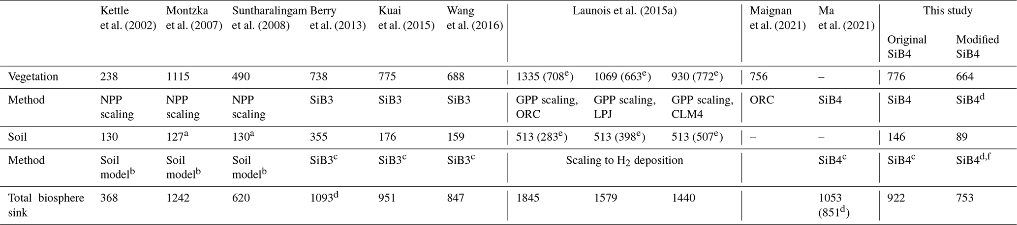
^a Adopted from Kettle et al. (2002). ^b Following Kesselmeier et al. (1999). ^c Scaled to heterotrophic CO₂ respiration. ^d Considering a variable mixing ratio. ^e After optimization. ^f Following Ogée et al. (2016).

2 Methodology

2.1 SiB4

The Simple Biosphere Model version 4 (SiB4) is a mechanistic, prognostic land surface model that integrates heterogeneous land cover, environmentally responsive prognostic phenology, dynamic carbon allocation, and cascading carbon pools from live biomass to surface litter to soil organic matter (Haynes et al., 2019a, b). SiB4 predicts vegetation and soil moisture states, land surface energy and water budgets, and the terrestrial carbon cycle. Rather than relying on satellite data to specify phenology as in SiB3, SiB4 simulates the terrestrial carbon cycle by using the carbon fluxes to determine the above- and belowground biomass, which in turn feeds back to impact carbon assimilation and respiration (Haynes et al., 2020). SiB4 predicts plant phenology, divided into different stages and allowing the change in photosynthetic activity over seasons through specified maximum RuBisCO velocities in each phenological stage. To classify land surface vegetation, SiB4 uses plant functional types (PFTs), which group plants according to their function and physical, physiological, and phenological characteristics. In addition to nine non-crop vegetation PFTs, SiB4 includes three specific crops (maize, soybeans, and winter wheat) and two generic crops (C₃ and C₄) following the crop phenology model developed by Lokupitiya et al. (2009). SiB4 includes land cover heterogeneity by simulating multiple PFTs per grid cell.

2.1.1 COS plant and soil uptake

COS plant uptake in SiB4 is based on the formulation of Berry et al. (2013) and is simulated as a series of conductances (g_t) from the leaf boundary layer to the site of COS hydrolysis in the mesophyll cells. These conductances include the conductance from canopy air to the leaf surface, or leaf boundary layer conductance (g_b); the stomatal conductance (g_s); and the internal conductance (g_cos). The latter represents both the diffusion of COS to the mesophyll cells and the efficiency of the leaf mesophyll carbonic anhydrase (CA) to hydrolyze COS. This leads to the following equation for the COS uptake rate by vegetation:

$$\begin{array}{}\text{(1)}& {\displaystyle }{F}_{\text{cos,veg}}=C_{\mathrm{a}}{\displaystyle \frac{\mathrm{1}}{\frac{\mathrm{1.94}}{g_{\mathrm{s}}}+\frac{\mathrm{1.56}}{g_{\mathrm{b}}}+\frac{\mathrm{1}}{g_{\text{cos}}}}}=C_{\mathrm{a}}{g}_t,\end{array}$$

where F_cos,veg is the COS vegetation uptake rate ($\mathrm{pmol}{\mathrm{m}}^{-\mathrm{2}}{\mathrm{s}}^{-\mathrm{1}}$) and C_a is the COS mole fraction in the canopy air space (pmol mol⁻¹) calculated from the mixed-layer COS mole fraction (standard 500 pmol mol⁻¹, but see Sect. 2.1.3.) taking into account uptake of COS by soil and vegetation in the previous time step. g_s and g_b are the respective stomatal and boundary layer conductances for water vapor ($\mathrm{mol}{\mathrm{m}}^{-\mathrm{2}}{\mathrm{s}}^{-\mathrm{1}}$) and are scaled to account for the different diffusivity rates of COS and H₂O (Seibt et al., 2010; Stimler et al., 2010). The stomatal conductance g_s is derived following the Ball–Berry photosynthesis–conductance model as modified by Collatz et al. (1992), and g_b follows the formulations described by Sellers et al. (1996). The internal conductance g_cos is assumed to scale with the maximum carboxylation rate of RuBisCO, V_max ($\mathrm{\mu }\mathrm{mol}{\mathrm{m}}^{-\mathrm{2}}{\mathrm{s}}^{-\mathrm{1}}$) (Berry et al., 2013), inspired by previous findings that both CA activity (Badger and Price, 1994) and mesophyll conductance (Evans et al., 1994) scale with V_max in C₃ species. In SiB4, V_max is calculated from V_max for carboxylation at 25 ^∘C ($V_{\mathrm{c},max\mathrm{25}}$) adjusted to canopy temperature (T_can) following Sellers et al. (1992):

$$\begin{array}{}\text{(2)}& {\displaystyle }{V}_{\text{max}}=V_{\mathrm{c},max\mathrm{25}}{\mathrm{2.1}}^{\mathrm{0.1}(T_{\text{can}}-\mathrm{298.0})}.\end{array}$$

g_cos is then described as function of V_COS that represents the CA activity:

$$\begin{array}{}\text{(3)}& {\displaystyle }\left\{\begin{array}{l}{g}_{\text{cos}}=\mathit{\alpha }\cdot V_{\text{COS}}\cdot F_{\text{LC}},\\ V_{\text{cos}}=V_{\text{max}}\cdot F_{\text{RZ}}\cdot \left(\frac{p}{p_{\text{0sfc}}}\right)\cdot \frac{T_{\text{can}}}{T_{\mathrm{0}}},\end{array}\right.\end{array}$$

where F_LC is a factor scaling the flux from a single leaf to the canopy that considers the canopy profile of absorbed photosynthetically active radiation (Sellers et al., 1996); F_RZ is the root zone water potential, an empirical scaling factor that reduces the biochemical activity when little soil moisture is available (e.g., during extended periods of drought); $p/p_{\text{0sfc}}$ adjusts the fluxes for altitude, where p is atmospheric pressure (hPa) and p_0sfc the reference surface pressure (1000 hPa); and $T_{\text{can}}/T_{\mathrm{0}}$ scales the flux to a reference temperature at T₀=273.15 K. A calibration term α was added to scale g_cos to COS flux observations of controlled gas exchange measurements (Stimler et al., 2010, 2011), which resulted in α=1200 for C₃ and α=13 000 for C₄ species (Berry et al., 2013). These numbers were later updated to α=1400 and α=8862 for C₃ and C₄ species, respectively, after reanalysis of the gas exchange data. Berry et al. (2013) already noted that the α value did not constrain the variability between plant species well, likely due to plant variability in CA activity and/or differences in mesophyll conductance. In Sect. 2.3 we explain how we use field measurements to explore whether we can refine α values for different plant functional types separately and to make α variable over time.

The enzyme CA is expressed in microbial communities in soils as well, leading to COS uptake by soils (e.g., Kesselmeier et al., 1999; Meredith et al., 2019). In SiB4, COS uptake in soils (hereafter called “the Berry soil model”) is coupled to heterotrophic CO₂ respiration under the assumption that in more productive regions there would be more litter and surface soil carbon for respiration, and these richer carbon environments would have more CA as well (Yi et al., 2007). Additionally, COS soil uptake in the model is regulated by diffusion, controlled by soil porosity and the fraction of water-filled pore space (Van Diest and Kesselmeier, 2008; Ogée et al., 2016; Sun et al., 2015; Whelan et al., 2016). Initial implementations of soil COS uptake made calculations for the entire soil column, but subsequent model versions considered only uptake in the top 20 cm of the soil (Wang et al., 2016), thereby decreasing global soil uptake estimates from 355 (Berry et al., 2013) to 159 Gg S yr⁻¹ (Wang et al., 2016). In the next section, we describe our update to SiB4 based on advances in our knowledge on COS soil exchange obtained during the last decade.

2.1.2 Mechanistic COS soil model

Field and laboratory experiments in the last decade have shown that COS is not only taken up by soil but also produced due to abiotic thermal degradation and photodegradation of soil organic matter and is especially enhanced in agricultural soils (Maseyk et al., 2014; Whelan and Rhew, 2015; Meredith et al., 2018; Kaisermann et al., 2018a). Besides COS soil production being enhanced in fertilized soils, COS uptake was shown to be diminished in fertilized soils (Kaisermann et al., 2018b). These effects of fertilization on soil COS exchange were initially not simulated in SiB4.

New empirical soil models (Whelan et al., 2016) and mechanistic models (Ogée et al., 2016; Sun et al., 2015) have been developed during the last decade. The mechanistic models describe the uptake and production pathways together with COS diffusion in a soil column. Ogée et al. (2016) derived a simplified analytical solution assuming a soil column with uniform temperature, soil moisture, and porosity and steady-state conditions for comparison against laboratory measurements. The model from Ogée et al. (2016), hereafter called “the Ogée soil model”, was then used by several laboratory studies to study patterns in uptake and production of COS in soils (Meredith et al., 2018, 2019; Kaisermann et al., 2018a, b). Due to these efforts, there are now reaction rate parameter values available for a range of biomes and land use types. Because these reaction rate values were derived by fitting the Ogée soil model on data from mesocosm experiments, they should be used in combination with this model to estimate ecosystem-scale soil COS fluxes. Also, compared to the COS soil model proposed by Sun et al. (2015), the steady-state solution of the Ogée soil model is computationally inexpensive and therefore more suitable for implementation in SiB4 for global COS soil flux calculations. In the following paragraphs we describe the implementation of the Ogée soil model in SiB4.

For field conditions (assuming a zero COS vertical gradient at the bottom of the soil layer and steady state), the COS soil flux ($\mathrm{mol}{\mathrm{m}}^{-\mathrm{2}}{\mathrm{s}}^{-\mathrm{1}}$) calculation simplifies to (Ogée et al., 2016)

$$\begin{array}{}\text{(4)}& {\displaystyle }{F}_{\text{COS,soil}}=\sqrt{kB\mathit{\theta }D}\cdot \left(C_{\mathrm{a}}-{\displaystyle \frac{z_{\mathrm{1}}^{\mathrm{2}}P}{D}}\left(\mathrm{1}-\text{exp}({\displaystyle \frac{z_p}{z_{\mathrm{1}}}}\right)\right),\end{array}$$

where k is the CA reaction rate (s⁻¹), B (cubic meters of water per cubic meter of air) is the solubility of COS in water that relates to Henry's law constant and depends on temperature, θ is the soil water content (m³ m⁻³), D is the soil COS diffusivity (cubic meters of air per meter of soil per second), C_a is the COS mole fraction at the soil–air interface, $z_{\mathrm{1}}^{\mathrm{2}}$ is $D/\left(kB\mathit{\theta }\right)$, and P is the COS production rate ($\mathrm{mol}{\mathrm{m}}^{-\mathrm{3}}{\mathrm{s}}^{-\mathrm{1}}$) that is uniform over depth z_p (here assumed to be 1.0 m). For details of the model calculations we refer readers to Ogée et al. (2016); here we provide the information specific to the implementation in SiB4. We assume C_a to be identical to the COS mole fraction in the canopy air space. While implementing and testing the model we recognized the strong dependence of the soil fluxes on soil porosity, choice of tortuosity functions, and the SiB4 soil layer selected for temperature and soil moisture. For the calculation of D we used the SiB4 soil porosity (m³ m⁻³; calculated from sand fractions following Lawrence and Slater, 2008) that accounts for the volume of ice in the soil. The simulated soil water content and soil temperature are taken from the top 5 cm soil layer, where most of the COS uptake takes place. D also depends on tortuosity functions that describe the tortuous movement through the air- or water-filled pore space. Several tortuosity functions are described in the literature, and also Ogée et al. (2016) acknowledged that the response of the soil COS fluxes to soil moisture varied with the chosen tortuosity functions. We chose the tortuosity functions of Deepagoda et al. (2011) for air and Millington and Quirk (1961) for water as these functions do not depend on a pore-size distribution parameter, which facilitates its implementation in SiB4.

COS is taken up in soils through hydrolysis in soil water, where the main consumption is enzymatic and thus dependent on soil CA enzyme activity. Here and following other studies (i.e., Ogée et al., 2016; Meredith et al., 2019), we expressed the CA reaction rate k relative to the uncatalyzed reaction rate (k_uncat) at a reference temperature (T_ref) and pH (here assumed constant at 4.5):

$$\begin{array}{}\text{(5)}& {\displaystyle }k=f_{\text{CA}}{k}_{\text{uncat}}{\displaystyle \frac{x_{\text{CA}}\left(T\right)}{x_{\text{CA}}\left(T_{\text{ref}}\right)}},\end{array}$$

where f_CA is the CA enhancement factor, k_uncat varies with soil pH according to Elliott et al. (1989), and x_CA(T) and x_CA(T_ref) are temperature response functions (Ogée et al., 2016).

Meredith et al. (2019) collected soils from 20 sites from different biomes. Using controlled laboratory measurements, they derived k_cat, k_uncat, and f_CA from a range of biomes and land use types. In SiB4 we used the biome-averaged f_CA from Meredith et al. (2019) for calculation of COS soil uptake across different PFTs (Table 2). Here, the f_CA for agricultural soils is substantially smaller than that of other vegetated biome types, thereby including the reduced COS uptake in fertilized (agricultural) soils (Kaisermann et al., 2018b).

The COS production was defined by Ogée et al. (2016) as a temperature response function modulated by the soil redox potential. Meredith et al. (2018) also measured COS production at a temperature range between 10 and 40 ^∘C for a range of biomes. Measurements were then fitted to an exponential model:

$$\begin{array}{}\text{(6)}& {\displaystyle }P=a\exp \left(b{T}_{\text{soil}}\right).\end{array}$$

We used this exponential temperature model and the biome-averaged a and b (Table 2) in our calculation of P in SiB4. We assume here that the controlled laboratory measurements by Meredith et al. (2018, 2019) can be used to estimate soil fluxes under field conditions. The higher value of a for agricultural soils (Table 2) allows for higher COS soil production in this soil type. Ideally, we would include production parameter values for wetland soils so that we take into account the typically large production that has been observed in wetland soils (Meredith et al., 2018; Whelan et al., 2013). However, SiB4 does not discriminate between oxic and anoxic (wetland) soils, which precluded the implementation of wetland-specific COS soil production.

Table 2 Biome-averaged uptake and production parameters after Meredith et al. (2018, 2019).

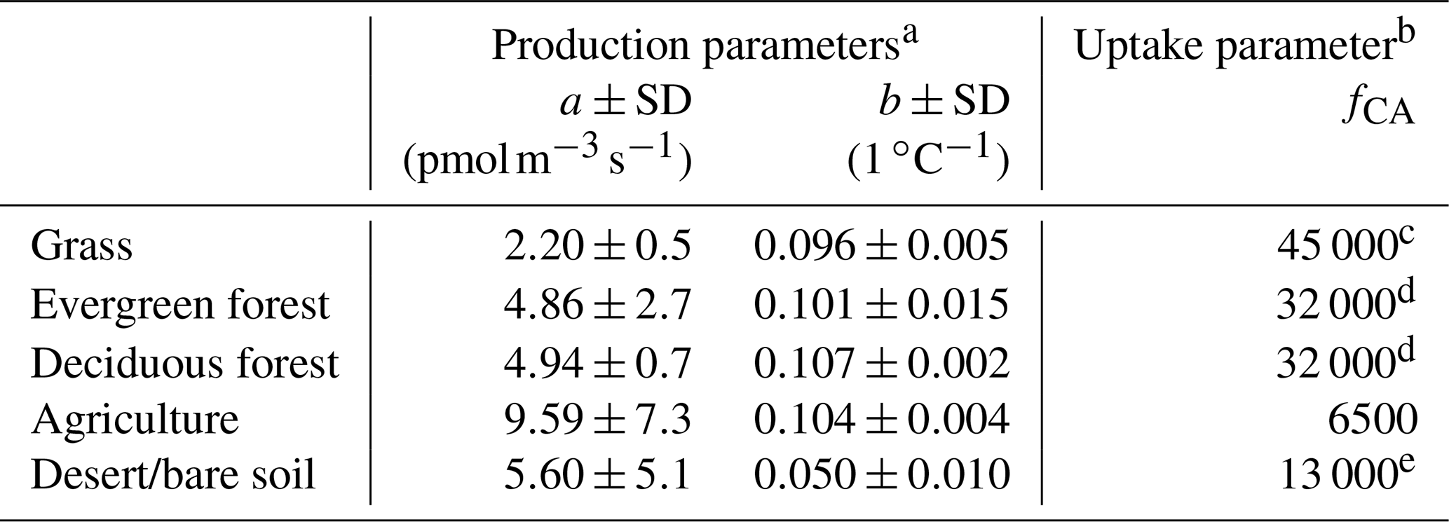
^a Based on Meredith et al. (2018). ^b Based on Meredith et al. (2019). ^c Measurements represent tropical grassland. ^d Measurements represent temperate coniferous and temperate broadleaf forests. ^e Measurements represent desert soil.

2.1.3 Variable atmospheric COS mole fractions

The atmospheric COS mole fraction in the planetary boundary layer affects both the COS vegetation and soil flux calculations (Eqs. 1 and 4). In SiB4 a standard constant “placeholder” COS mole fraction of 500 pmol mol⁻¹ is used. Ma et al. (2021) estimated that the global biosphere sink would decrease from 1053 to 851 Gg S yr⁻¹ if the fixed COS mole fraction were replaced with monthly mean fields that account for the drawdown of COS near the surface in the peak growing season. We thus changed the prescribed COS mole fraction from a fixed value to one varying in space and time, including seasonal and diurnal variability. To this end we used the surface COS mole fraction fields at a global resolution of $\mathrm{4}{}^{\circ }\times \mathrm{6}{}^{\circ }$ (latitude × longitude) at 3-hourly time steps as retrieved from an atmospheric transport inversion performed with TM5-4DVAR by Ma et al. (2021) using the chemistry transport model TM5 in which COS exchange was recently implemented. Measurements of atmospheric COS mole fractions at 14 sites from the National Oceanic and Atmospheric Administration (NOAA) flask network (Montzka et al., 2007) were used to optimize the sources and sinks of COS. We used global 2D surface layer fields of COS mole fractions resulting from these optimized sources and sinks as they were optimally consistent with the available COS flask observations for the period 2016–2018. We repeated the average over those years as input to the SiB4 mixed-layer COS mole fraction for each year in the simulation (see global maps of monthly mean surface COS mole fractions in Fig. S13 in the Supplement of Ma et al., 2021). In the inversion of Ma et al. (2021), the changing (e.g., lower) COS mole fractions would lead to lower COS uptake rates but would in turn also lead to a smaller drop in COS mole fractions; this feedback is currently not accounted for.

2.1.4 Simulations

We used meteorological data from the Modern-Era Retrospective Analysis for Research and Applications, version 2 (MERRA-2), which are available from 1980 onwards (Gelaro et al., 2017), as meteorological forcing to SiB4. To ensure realistic rainfall, the convective and large-scale precipitation values were scaled such that the monthly total rainfall matches with the monthly precipitation in the Global Precipitation Climatology Project, Version 1.2 product (Huffman et al., 2001; Baker et al., 2010; Haynes et al., 2019a, b). Up to 10 PFTs per grid cell (at $\mathrm{0.5}{}^{\circ }\times \mathrm{0.5}{}^{\circ }$ resolution) are prescribed following PFT maps based on MODIS data (Lawrence and Chase, 2007). The soil characteristics such as the sand fraction (used for the calculation of soil porosity) are provided by the International Geosphere-Biosphere Programme (IGBP) Global Soil Data Task Group (2000).

We ran SiB4 from 2000 to 2020, and the simulations were preceded by a spinup iterating five times over the years 2000–2020 using an accelerated equilibrium approach (Haynes et al., 2019b) to initialize the carbon pools to reach a steady state. CO₂ mole fractions were held constant at 370 µmol mol⁻¹ during spinup and simulations. Research is ongoing to implement an accurate representation of the effect of CO₂ fertilization in SiB4. We performed two sets of four simulations (global and site level) with the same driver data and settings but with a different temporal resolution of the output: (1) for global simulations, we used monthly averaged output. Moreover, SiB4 simulates multiple PFTs per grid cell. These were averaged, weighted by the fraction of land area occupied by each PFT. (2) To compare SiB4 with site observations (listed in Table 3), we run SiB4 with 3-hourly output for only the grid cells (at $\mathrm{0.5}{}^{\circ }\times \mathrm{0.5}$^∘ resolution) in which the sites are located. For comparison with observations we selected the PFT that best represents the measurement site. For these site comparisons we use MERRA-2 meteorological data (instead of local meteorological observations) to provide consistency in data collection, availability, and application across sites and for consistency with the global run.

We run SiB4 with four different configurations:

1. the original SiB4 containing the standard COS mole fraction of 500 pmol mol⁻¹ and the Berry soil model (SiB4_500_Berry),

2. the Ogée soil model and the standard COS mole fraction of 500 pmol mol⁻¹ (SiB4_500_Ogee),

3. the Berry soil model and variable COS mole fractions (SiB4_var_Berry), and

4. the Ogée soil model and variable COS mole fractions (SiB4_var_Ogee).

2.2 Field observations

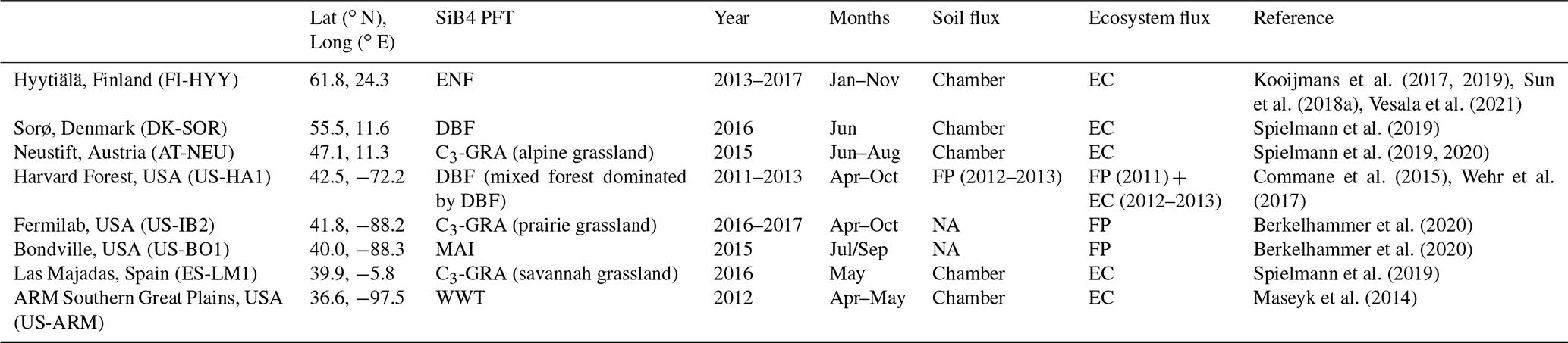
We use existing field observations for comparison with the SiB4 simulations. Several studies have collected field data in the last 2 decades, and we used those sites where continuous hourly measurements of ecosystem COS fluxes are available for at least a month. The site name abbreviations, their locations, some of their characteristics, and basic information on the observations are summarized in Table 3. The locations of the sites are indicated in Fig. S1 in the Supplement. The measurements represent evergreen needleleaf forest (ENF); deciduous broadleaf forest (DBF); maize (MAI); winter wheat (WWT); and C₃ grasslands (C₃-GRA), more specifically alpine grassland, prairie grassland, and savannah grassland.

All COS observations were made at FLUXNET, ICOS, or AmeriFlux sites with the benefit that additional long-term measurements of CO₂ and water exchange (Pastorello et al., 2020) are often available (see Table S1 in the Supplement for an overview), allowing the evaluation of the SiB4 phenology when COS flux observations do not extend to a full growing season. Most of the ecosystem observations were made using the eddy-covariance (EC) technique. Kohonen et al. (2020) summarized the different EC processing steps used by the different studies. Only at US-IB2, US-BO1, and for a part of the dataset at US-HA1 (in 2011) are the ecosystem fluxes derived by COS concentration gradients using the flux-profile (FP) technique (Berkelhammer et al., 2020; Commane et al., 2015). The ecosystem fluxes determined by the EC technique can be biased due to storage (typically depletion) of COS in the canopy airspace under limited turbulent mixing. The air depleted in COS can then suddenly be captured by the EC system when turbulence is enhanced in the morning. Ecosystem fluxes therefore ideally need to be corrected for such storage change. We corrected the ecosystem fluxes for storage of COS in the canopy airspace using collocated canopy COS profile measurements when available (FI-HYY and US-HA1). More details on the storage flux calculation can be found in Kooijmans et al. (2017).

Most of the selected sites have in situ COS soil flux observations available for at least a part of the total measurement period so that the COS uptake by vegetation can be derived from observed ecosystem fluxes. Measurements were collected using soil chambers, except at US-HA1, where atmospheric profile measurements near the surface were used to calculate the soil fluxes in 2012 and 2013.

Measurement datasets also include COS mole fractions above the canopy (except for US-ARM). These measurements have been calibrated against the NOAA-2004 COS calibration scale. Only at US-HA1 are the COS mole fractions not calibrated (Commane et al., 2015), but they are validated against COS flask measurements at the station, which is part of the NOAA flask measurement network (Montzka et al., 2007).

For further details about the site characteristics and measurement and processing procedures, we refer to the original data publications as reported in Tables 3 and S1 in the Supplement.

For evaluation of the model against observations, we calculate the mean bias error (MBE, $\mathrm{pmol}{\mathrm{m}}^{-\mathrm{2}}{\mathrm{s}}^{-\mathrm{1}}$) and root mean square error (RMSE, $\mathrm{pmol}{\mathrm{m}}^{-\mathrm{2}}{\mathrm{s}}^{-\mathrm{1}}$) for monthly, daytime, and nighttime average fluxes.

Table 3 Site and measurement information of field observations that are used for comparison with SiB4. Sites are shown from high to low latitude. PFTs covered by the sites are evergreen needleleaf forest (ENF), deciduous broadleaf forest (DBF), C₃ grassland (C₃-GRA), maize (MAI), and winter wheat (WWT). The ecosystem and soil flux measurement techniques are indicated as eddy-covariance (EC), flux-profile (FP), and chamber measurements or are not available (NA). Mean annual temperature and mean annual precipitation are shown in Table S1.

2.3 Calibration factor α

Berry et al. (2013) used the calibration factor α to scale g_cos to match the simulated COS vegetation flux with laboratory measurements. They noted that the α value did not constrain the variability between plant species well, likely due to plant variability in CA activity and/or mesophyll conductance. Here, we derived α_obs from COS field measurements; however, as α_obs still contains several SiB4-simulated parameters, it is not strictly an observationally derived value. This analysis is meant to explore its variability over time and the necessity to define α values specifically for different PFTs. We did not retain α_obs for global simulations.

We derived g_t from measurements of canopy vegetation fluxes ($F_{\text{COS,veg}}=\text{ecosystem}-\text{soil fluxes}$) and simulated COS mole fractions in the canopy airspace C_a:

$$\begin{array}{}\text{(7)}& {\displaystyle }{g}_{t,\text{obs}}={\displaystyle \frac{F_{\text{COS,veg}}}{C_{\mathrm{a}}}}.\end{array}$$

Then, rewriting Eqs. (1) and (3) and adopting g_s, g_b, and g_cos from SiB4 site simulations, we calculated α_obs as

$$\begin{array}{}\text{(8)}& {\displaystyle }{\mathit{\alpha }}_{\text{obs}}={\displaystyle \frac{-\mathrm{1}}{\frac{V_{\text{cos}}}{g_{t,\text{obs}}}\left(g_{t,\text{obs}}\frac{\mathrm{1.94}}{g_{\mathrm{s}}}+g_{t,\text{obs}}\frac{\mathrm{1.56}}{g_{\mathrm{b}}}-\mathrm{1}\right)}}.\end{array}$$

α_obs was calculated for daytime hours (10:00–15:00 LT) in periods with photosynthetically active vegetation, which excludes data points of FI-HYY when plants are dormant in winter (November to April) and after the simulation of harvest at US-ARM. Raw α_obs data points were considered outliers when their values extended 1.5 times the 25th–75th percentile range outside the quartiles and were removed from the analysis.

This analysis requires that field measurements of ecosystem and soil fluxes are available. Under the assumption that both V_max (and thus photosynthesis) and the soil flux are accurately simulated, the application of α_obs would result in simulated COS vegetation fluxes that match with observations.

3 Results and discussion

First, we evaluate the SiB4 COS flux against observations (Sect. 3.1). The accuracy of the modeled ecosystem flux is controlled by several factors, such as the accuracy in leaf phenology, differences in accuracy of the daytime and nighttime COS vegetation flux, the accuracy of the soil flux (of both the Berry and the Ogée soil models), and the sensitivity to atmospheric COS mole fractions. We discuss the role of each of these factors in the evaluation of SiB4 biosphere fluxes against observations. All results are based on the standard α values of 1400 and 8862 for C₃ and C₄ species, respectively. We present COS fluxes relative to the atmosphere (i.e., negative values indicate uptake by the ecosystem). Next, we study the variability in α_obs between different PFTs and across seasons (Sect. 3.2) to investigate remaining model–data mismatches in the COS vegetation flux that could potentially be solved by re-calibrating α. Finally, we present global estimates of the COS biospheric sink with different model configurations (Sect. 3.3).

3.1 SiB4 COS flux evaluation and sensitivity

3.1.1 Seasonal variability

Simulated COS ecosystem fluxes capture the seasonal variation in monthly averaged observations (Fig. 1), with similar results for vegetation fluxes alone (Fig. S2 in the Supplement). Specifically, simulated COS uptake peaked in summer, as was observed at the three sites that contain COS flux measurements across different seasons (Fig. 1a, d, and e). At the other sites, COS ecosystem fluxes were only measured during one part of the growing season. Therefore, we also used multi-year NEE, GPP, and latent heat flux (LE) from EC sites to evaluate the SiB4 phenology, which affects both CO₂ and COS seasonality (Figs. S3–S5 in the Supplement).

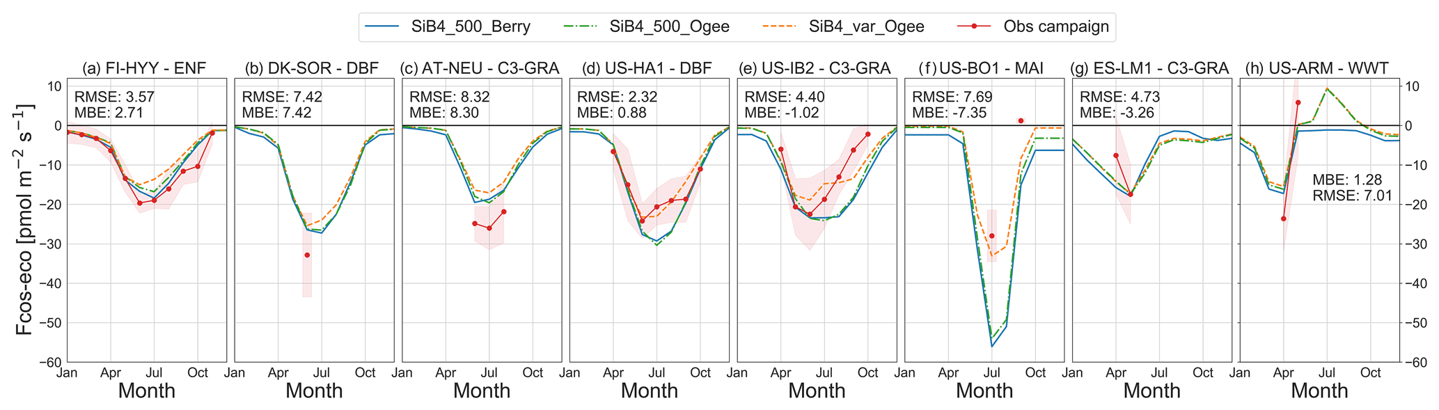
Figure 1 Comparison of ecosystem COS flux seasonal cycles of observations (red) with different SiB4 model runs: the original SiB4 with 500 pmol mol⁻¹ COS and the original Berry soil model (SiB4_500_Berry, solid blue), a run with variable COS mole fractions and the Ogée soil model (SiB4_var_Ogee, dashed orange), and a run with 500 pmol mol⁻¹ COS and the Ogée soil model (SiB4_500_Ogee, dash-dotted green). Monthly averages are shown with the 1σ spread around the mean of observations. Negative values indicate uptake of COS by the ecosystem, while positive values indicate COS emissions. The model simulations are from the same year(s) in which observations were made. The MBE and RMSE ($\mathrm{pmol}{\mathrm{m}}^{-\mathrm{2}}{\mathrm{s}}^{-\mathrm{1}}$) are given for monthly average fluxes of the SiB4_var_Ogee run. Sites are presented from high to low latitude.

Based on the NEE, GPP, and LE observations (Figs. S3–S5), the start and end of the growing season are typically well captured by the SiB4 simulations. The timing and length of the growing season for grassland sites has been previously evaluated by Haynes et al. (2019b) using remotely sensed leaf area index and showed that SiB4 was capable of simulating growing season timing and variability across temperature and precipitation gradients. Also, the timing of maximum NEE and GPP, which differs by PFT and climatic regions, was well captured; e.g., simulated and observed NEE and GPP peak in spring at the savannah grassland site ES-LM1 and at the winter wheat site US-ARM. All other sites show an observed and simulated summer maximum carbon uptake. Only AT-NEU is an exception, with SiB4 predicting the peak net CO₂ uptake too late into the summer compared to the observations, which can be explained by grass cutting that was not included in SiB4. Crop harvesting was included in SiB4, but the exact timing was difficult to simulate due to local weather events and considerations other than crop ripening. For example, at the US-ARM site the winter wheat harvest was on average simulated at DOY 136 for the years 2000–2019, close to the actual moment of harvest in 2012: DOY 145 (Maseyk et al., 2014). However, for 2012 (the year matching with COS flux observations), the model simulates harvest almost 4 weeks earlier (DOY 118) than was actually the case, possibly because in 2012 the meteorological forcing data prescribed on average 14 % higher daytime temperatures than observed, while in other years they were on average only 3 % higher than observations.

For the sites where COS fluxes were only measured in one part of the growing season, we assume that the timings of seasonal patterns in COS assimilation were well captured since seasonal patterns in NEE, GPP, and LE are properly simulated (Figs. S3–S5) and the model scales the CA activity with V_max and g_s with GPP.

We generally found larger underestimations of the ecosystem COS exchange at the higher latitudes (FI-HYY, DK-SOR, AT-NEU; Fig. 1a–c), which is consistent with findings by Ma et al. (2021), who found a missing sink at the higher latitudes that required uptake larger than in the inversion a priori model (i.e., SiB4) in summer (their Fig. 4b). The model–observation biases that we see in the ecosystem COS fluxes are consistent with biases in GPP for some sites. For example, the underestimation of the COS ecosystem flux at DK-SOR, AT-NEU, and FI-HYY is consistent with underestimations of GPP (Fig. S4a–c), which will be further discussed in Sect. 3.1.3.

3.1.2 Effects of varying atmospheric COS mole fractions

Modifying the COS mole fractions to vary spatially and temporally significantly improved the comparison with observations in North America, as seen from the orange (variable COS) and green (fixed COS) line in Fig. 1d–f. Generally, COS mole fractions are lower in the second half of the growing season (Fig. S6 in the Supplement), leading to lower COS uptake in that period. When a variable COS mole fraction was used, the MBE value in July–August improved from 9.0 to 2.0 $\mathrm{pmol}{\mathrm{m}}^{-\mathrm{2}}{\mathrm{s}}^{-\mathrm{1}}$ at US-HA1, from 7.2 to −0.9 $\mathrm{pmol}{\mathrm{m}}^{-\mathrm{2}}{\mathrm{s}}^{-\mathrm{1}}$ at US-IB2, and from 28.6 to 5.4 $\mathrm{pmol}{\mathrm{m}}^{-\mathrm{2}}{\mathrm{s}}^{-\mathrm{1}}$ at US-BO1. The influence of the COS mole fraction on the biosphere flux was largest at sites within or close to the Corn Belt in the Midwestern USA with strong biosphere COS uptake (see also Fig. 5) that therefore have the largest summertime drop in COS mole fractions (Fig. S6d and e) or the lowest COS mole fraction in general (Fig. S6f). The large COS uptake by maize (corn) is confirmed by the observed COS fluxes reaching ∼70 $\mathrm{pmol}{\mathrm{m}}^{-\mathrm{2}}{\mathrm{s}}^{-\mathrm{1}}$ at midday (local time, Fig. S8 in the Supplement). In this region, the lower COS mole fractions lead to reduced COS uptake but would in turn lead to a smaller drop in COS mole fractions. As COS uptake and COS mole fractions are interconnected, SiB4 should ideally be directly coupled to an atmospheric transport model.

At other sites (Europe) the variable COS mole fractions did not improve the model–observation bias but instead caused a slightly larger underestimation by the model. The comparison of COS mole fractions from the TM5-4DVAR inversion against those observed at the measurement sites (Fig. S6) did not indicate that the COS mole fractions were consistently better simulated over North America than over Europe. These results imply that the underestimation of COS fluxes over Europe is not likely caused by an underestimation of the COS mole fractions. On the other hand, the COS mole fractions observed at the measurement sites are not as consistently calibrated as the NOAA measurement network.

3.1.3 Diurnal cycles

The monthly average ecosystem COS fluxes (Fig. 1) included both day- and nighttime fluxes and soil and vegetation fluxes, which may each have their own biases. Figure 2 shows model–observation differences in vegetation COS uptake separated by day- and nighttime, defined as 10:00–15:00 and 21:00–03:00 LT, respectively. These day- and nighttime definitions exclude transitions between day and night (see diurnal cycles in Figs. S8 and S9 in the Supplement). On average across all stations, simulated daytime uptake between April through October was lower than the observations by 1.9±6.5 $\mathrm{pmol}{\mathrm{m}}^{-\mathrm{2}}{\mathrm{s}}^{-\mathrm{1}}$ (8±27 %). Even though the average model–observation difference is small, there is substantial variability between sites. The underestimation of daytime COS uptake of 19.3 $\mathrm{pmol}{\mathrm{m}}^{-\mathrm{2}}{\mathrm{s}}^{-\mathrm{1}}$ (34 %) at DK-SOR was exceptionally large, consistent with the underestimation of daytime GPP in the same period (13.1 $\mathrm{\mu }\mathrm{mol}{\mathrm{m}}^{-\mathrm{2}}{\mathrm{s}}^{-\mathrm{1}}$, 34 %). The COS measurements at DK-SOR were made in June 2016, a period that was warmer than average at this site. As a result, observed GPP was 25 % higher in June 2016 compared to the 1996–2018 average (Fig. S4b). However, SiB4 simulates only a 7 % higher GPP in June 2016 compared to the 1996–2018 average. At the same time, LE is overestimated (Fig. S5b). A SiB4 run with observed meteorology as driver input showed a similar GPP anomaly to when the MERRA-2 driver input was used (Fig. S7a). The fact that SiB4 is not able to capture the GPP anomaly is thus not due to the driver data used. These results point to an underestimation of the RuBisCO and CA enzyme activity and thus g_cos, rather than g_s, as LE is not underestimated but instead overestimated. Also at AT-NEU and FI-HYY the underestimation of COS vegetation uptake was consistent with underestimations of simulated GPP against long-term time series (Fig. S4a and c), with a 9 % underestimation of the COS vegetation flux and 13 % underestimation of GPP at FI-HYY in the months June to August. At US-ARM we saw a switch from underestimation to overestimation of daytime vegetation COS uptake over the months April and May, which may be due to COS emissions from components other than the soil, possibly associated with senescing vegetation (Geng and Mu, 2005; Maseyk et al., 2014), which is currently not represented in SiB4 (nor in other models). Overall, we found large variability in model–observation biases between sites, but no clear distinctions emerge from different PFTs for daytime fluxes.

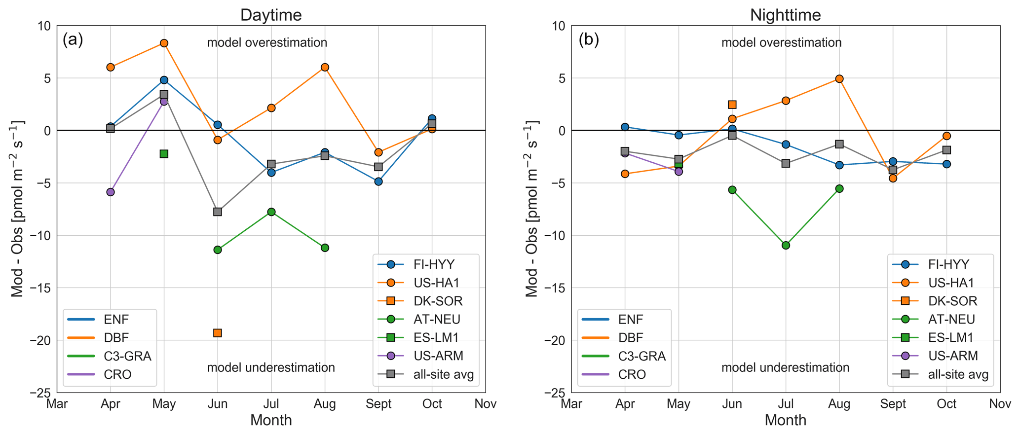
Figure 2 Difference between model simulations and observations of monthly average COS vegetation fluxes (ecosystem–soil) for daytime data (10:00–15:00 LT, a) and nighttime data (21:00–03:00 LT, b). As ecosystem and soil fluxes are needed to obtain the vegetation flux, only sites with these data available are shown here. The model simulations were made with a variable COS mole fraction and the Ogée soil model (SiB4_var_Ogee). Data are colored by PFT (i.e., ENF, DBF, C₃-GRA, and crops (CRO)).

The simulated nighttime uptake was too small by an average of 2.1±3.4 $\mathrm{pmol}{\mathrm{m}}^{-\mathrm{2}}{\mathrm{s}}^{-\mathrm{1}}$ (35±57 %). Observed nighttime uptake was on average 25 % of the daytime uptake across sites between May–September, with the largest uptake at AT-NEU (11.0 $\mathrm{pmol}{\mathrm{m}}^{-\mathrm{2}}{\mathrm{s}}^{-\mathrm{1}}$), ES-LM1 (6.9 $\mathrm{pmol}{\mathrm{m}}^{-\mathrm{2}}{\mathrm{s}}^{-\mathrm{1}}$), and FI-HYY (5.9 $\mathrm{pmol}{\mathrm{m}}^{-\mathrm{2}}{\mathrm{s}}^{-\mathrm{1}}$). The small flux values during nighttime make the model–observation comparison sensitive to the different correction and processing procedures that were used for the different datasets. Ecosystem fluxes were only storage-corrected for FI-HYY and US-HA1. Kooijmans et al. (2017) showed for FI-HYY that nighttime storage fluxes were on average ∼1 $\mathrm{pmol}{\mathrm{m}}^{-\mathrm{2}}{\mathrm{s}}^{-\mathrm{1}}$ in summer. Additionally, some datasets are filtered based on a friction velocity threshold, while others are not. Kooijmans et al. (2017) noted that filtering data based on the friction velocity might bias the data towards higher nighttime COS uptake as the uptake can be expected to be limited by the COS gradient at the leaf boundary layer under low-turbulence conditions. Given these differences between datasets and the typically large random noise of COS flux measurements, the average underestimation may not be significant overall. Still, we found a substantial underestimation of the nighttime COS uptake at the C₃-GRA sites AT-NEU and ES-LM1 and an overestimation in summer at the DBF sites US-HA1 and DK-SOR. These biases might point to an inaccurate intercept of the Ball–Berry stomatal conductance model (g₀, i.e., when GPP is (near) zero) in SiB4, which is currently set to 10 $\mathrm{mmol}{\mathrm{m}}^{-\mathrm{2}}{\mathrm{s}}^{-\mathrm{1}}$ for all PFTs in SiB4, except for C₄ grasslands and crop types (both C₃ and C₄) (40 $\mathrm{mmol}{\mathrm{m}}^{-\mathrm{2}}{\mathrm{s}}^{-\mathrm{1}}$). Observed g₀ values at AT-NEU (10–65 $\mathrm{mmol}{\mathrm{m}}^{-\mathrm{2}}{\mathrm{s}}^{-\mathrm{1}}$; Wohlfahrt, 2004) are mostly higher than the 10 $\mathrm{mmol}{\mathrm{m}}^{-\mathrm{2}}{\mathrm{s}}^{-\mathrm{1}}$ used in SiB4 and support the hypothesis that the SiB4 g₀ is too low for this site. Similarly, estimates of the nighttime dark-adapted conductance (g_dark) at US-HA1 (3.1 $\mathrm{mmol}{\mathrm{m}}^{-\mathrm{2}}{\mathrm{s}}^{-\mathrm{1}}$; Wehr et al., 2017) point to a smaller value than used in SiB4 and could explain part of the overestimation of nighttime COS uptake at this site when it is assumed that g₀ is representative of g_dark (Lombardozzi et al., 2017). These examples show that observations could help to obtain g₀ values for SiB4. Lombardozzi et al. (2017) made a literature overview of reported g₀ values per PFT and showed that g₀ was typically several times larger than the value of 10 $\mathrm{mmol}{\mathrm{m}}^{-\mathrm{2}}{\mathrm{s}}^{-\mathrm{1}}$ currently used in SiB4. We adopted the g₀ values of Lombardozzi et al. (2017) in SiB4 to test the effect of a modified g₀ setting on the nighttime COS vegetation flux (see Table S2 and Fig. S10 in the Supplement). Using these updated g₀ values, the simulated nighttime COS uptake for C₃-GRA improved at AT-NEU but had larger biases for other sites and PFTs, especially DBF (Fig. S10). As the g₀ values from Lombardozzi et al. (2017) did not consistently improve the nighttime COS uptake, we did not adopt these as standard SiB4 settings.

3.1.4 Soil fluxes

The original SiB4 soil model scaled COS soil fluxes to heterotrophic CO₂ respiration, leading to COS uptake rates peaking at high temperatures in summer (Figs. 3 and S11 in the Supplement) and in conditions with sufficient soil moisture (Figs. 3g and S12g in the Supplement). The Ogée soil model also simulated COS uptake peaking at high temperatures and lower uptake rates in winter compared to the Berry soil model (Fig. 3). In general, the COS uptake simulated by the Berry soil model matched well with observations at forest sites (Fig. 3a, b, and d), possibly because their approach was following a study on forest soils (Yi et al., 2007). The Ogée soil model underestimated the COS uptake at FI-HYY (Fig. 3a) but was closer to observations at the other forest sites US-HA1 and DK-SOR (Fig. 3b and d). The observed high soil COS uptake in April at FI-HYY is possibly related to snowmelt and thawing of the soil, and neither model captures this effect on soil COS exchange.

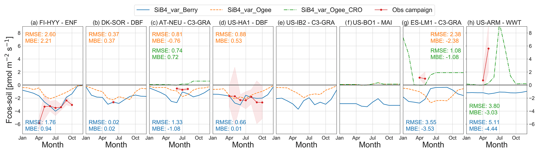
Figure 3 Comparison of COS soil flux seasonal cycles of observations (red) with different SiB4 model runs: SiB4_var_Berry (solid blue); SiB4_var_Ogee with the simulation representing the PFT type as indicated in the plot titles (dashed orange); and SiB4_var_Ogee_CRO with the simulation representing agricultural soil (Table 2) for sites AT-NEU, US-BO1, ES-LM1, and US-ARM (dash-dotted green). No in situ observations of soil COS fluxes are available for US-IB2 and US-BO1. Monthly averages are shown with the 1σ spread around the mean for observations. The model simulations are from the same year(s) in which observations were made. Negative values indicate uptake of COS by the ecosystem, while positive values indicate COS emissions. The MBE and RMSE ($\mathrm{pmol}{\mathrm{m}}^{-\mathrm{2}}{\mathrm{s}}^{-\mathrm{1}}$) are given for monthly average fluxes for all model runs in their respective color. Sites are presented from high to low latitude.

Soil COS emissions were observed at ES-LM1 and US-ARM. US-ARM was an agricultural site where emissions may build up after the peak growing season in the period associated with senescence and harvest (Maseyk et al., 2014). The Berry soil model did not simulate soil COS emissions (Fig. 3h). In contrast, the increase in COS emissions at the agricultural site US-ARM was simulated by the Ogée soil model, although the increase in the emissions started later than in the observations. The soil emissions of COS were not simulated at the C₃-GRA site ES-LM1. However, the soil at ES-LM1 was fertilized (Weiner et al., 2018), as well as that AT-NEU (Spielmann et al., 2020), which makes these sites more representative of agricultural soils than grassland soils. When ES-LM1 was simulated as an agricultural soil (the same code but with different uptake and production parameter values; see Table 2), the model showed COS emissions that were more consistent with observations (green line in Fig. 3g). Also, the simulated fluxes at the AT-NEU site became smaller and were in better agreement with observations when the site was considered an agricultural soil.

The accuracy of simulations of soil COS emissions depends on the accuracy of the production parameter a. The standard deviation of the production parameter a (7.3) is relatively large for agricultural soils compared to other soil types (Table 2) and is an indication of the uncertainty in using a single production value in SiB4. Reasons for this uncertainty can be the local variability in soil characteristics like nitrogen content, which has been shown to correlate well with COS production rates (Kaisermann et al., 2018b). Moreover, soil moisture and soil temperature were important parameters in the calculation of the COS soil flux. In general, we found that the variability and absolute values of soil moisture and especially soil temperature were well captured by SiB4. We found a MBE across all sites of 0.01 m³ m⁻³ and 0.1 ^∘C (RMSE 0.06 m³ m⁻³ and 2.1 ^∘C) for soil moisture and temperature, respectively, calculated over all years available from the EC sites. Also, Smith et al. (2020) showed that SiB4 was capable of reproducing the drop in soil moisture as a result of a regional drought in Europe, albeit with a delay. We did not find consistent patterns in model–observation biases of the soil COS fluxes that were consistent with those of soil moisture or temperature (Figs. S11 and S12). Still, the soil moisture observations at US-ARM show a sharper drop in spring than the simulations (Fig. S12h), which could explain why the simulations show a delayed onset of soil COS emissions. Moreover, the exact role of thermal and photo-production of COS remains uncertain, as well as the interaction with soil organic matter and litter, and thereby limits the accuracy of soil COS production simulations (Maseyk et al., 2014; Whelan and Rhew, 2015; Meredith et al., 2018; Kaisermann et al., 2018a).

Overall, changing from the Berry soil model to the Ogée soil model had a relatively small effect on monthly average ecosystem fluxes (see SiB4_500_Berry (blue) and SiB4_500_Ogee (green) in Fig. 1), except for agricultural sites, where the Berry soil model lacked COS soil emissions that contribute to fluxes at those sites.

3.2 Calibration factor α

The calibration factor α was derived to scale g_cos to match SiB4 COS plant assimilation with COS flux observations of laboratory leaf gas exchange measurements (Berry et al., 2013). The α_obs values that we derived based on field measurements of COS ecosystem and soil fluxes, together with simulated g_cos, g_s, and g_b and V_COS, are close to the value 1400 (Fig. 4), which supports the initial calibration by Berry et al. (2013) using laboratory leaf gas exchange measurements. At the same time, we found α_obs to vary in time and between sites (Fig. 4), indicating that a single α value was not able to capture the variation in measured COS vegetation fluxes across sites and seasons. The average summertime α_obs (June–August) of 1616±562 was 15 % higher than the current value of 1400. This was consistent with our findings that, on average, SiB4 underestimates COS biosphere fluxes with both a variable and a constant COS mole fraction (Sect. 3.1.3). We did not find patterns in α_obs that apply to all PFTs in the same way that would have helped to update α in SiB4. However, for DBF and C₃-GRA sites we observed that the 2-weekly average α_obs typically goes down with increasing air temperature for temperatures above ∼16 ^∘C (Fig. S13 in the Supplement). This observation requires further investigation from hourly data points and will be further discussed in our recommendations (Sect. 4.3).

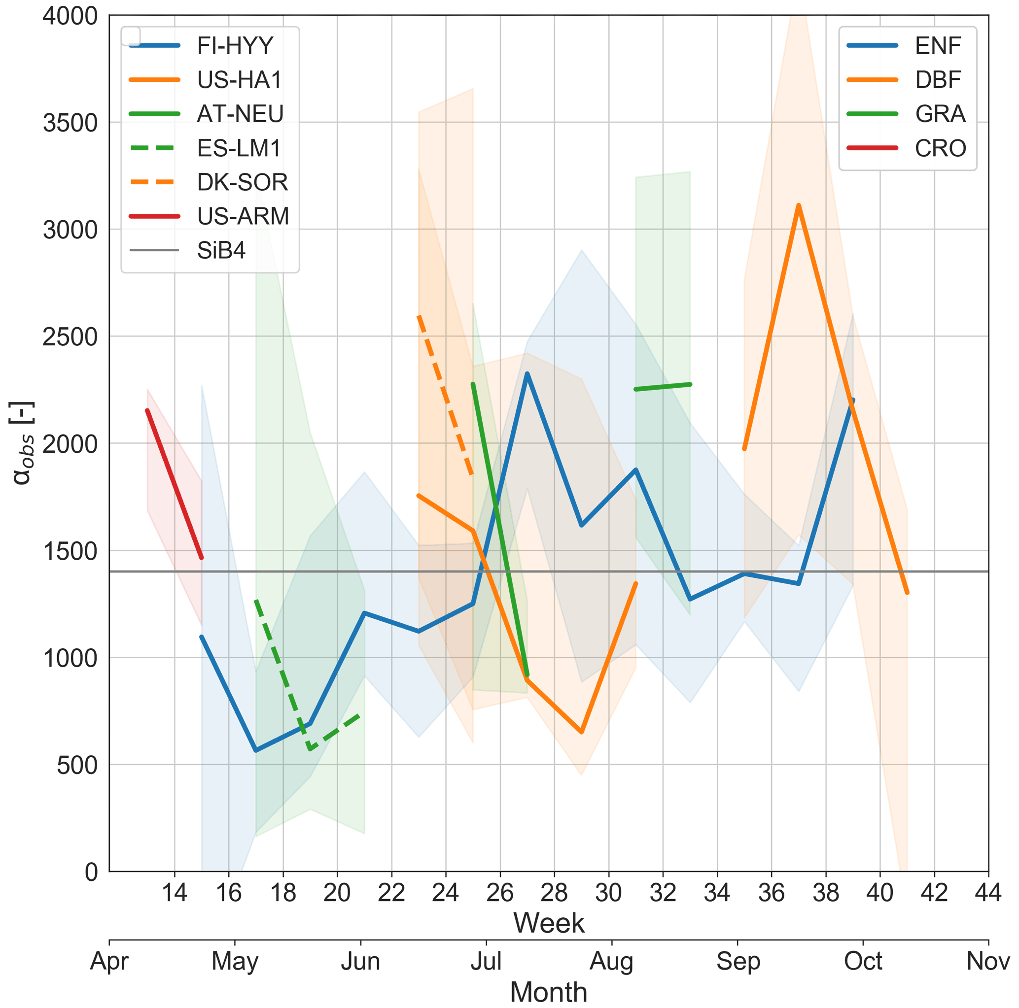
Figure 4 Seasonal change in (2-weekly) median observation-based calibration factor α (α_obs; see Eq. 10) per site in which colors are separated by PFT. The shaded areas represent the 25th–75th percentiles.

3.3 Global biospheric COS sink

The simulated global patterns in COS uptake were similar to those of GPP (Fig. S14 in the Supplement), due to the modeled vegetation COS uptake being coupled to GPP through the RuBisCO enzyme activity and stomatal conductance. Globally, the largest portion of COS uptake took place in tropical regions of South America, Africa, and Asia (Fig. 5). In the Northern Hemisphere (NH), COS was mainly taken up during the summer months (Fig. 5b). The spatial distribution of COS uptake was also similar to that presented by Maignan et al. (2021) based on ORCHIDEE simulations. Using the original SiB4, i.e., the original Berry soil model and fixed 500 pmol mol⁻¹ COS mole fractions, the global COS biosphere sink amounts to 922±11 (mean ± SD) Gg S yr⁻¹ over the years 2000–2020 with no substantial trend. Of the total COS biosphere sink, 146 Gg S yr⁻¹ was due to soil uptake (Table 1). The change from the original Berry soil model to the Ogée soil model lowered the soil uptake in most regions globally (Figs. 6a and S15 in the Supplement). The tropical soil COS uptake reduced from ∼4–5 to ∼2–3 $\mathrm{pmol}{\mathrm{m}}^{-\mathrm{2}}{\mathrm{s}}^{-\mathrm{1}}$. In the NH, the soil uptake is also reduced due to the contributions of COS production in agricultural soils. The global COS soil sink thereby reduced by 29 % from 146 to 104 Gg S yr⁻¹ when we changed from the original Berry soil model to the Ogée soil model, but this represents only a 5 % reduction in the total COS biosphere sink. On the other hand, moving from a fixed to a spatially and temporally varying COS mole fraction caused an additional reduction in the global COS biosphere sink to 753 Gg S yr⁻¹ (Figs. 6b and S16 in the Supplement). This 15 % reduction relative to a simulation with a constant and spatially uniform 500 pmol mol⁻¹ COS mole fraction illustrates the importance of accounting for varying COS mole fractions.

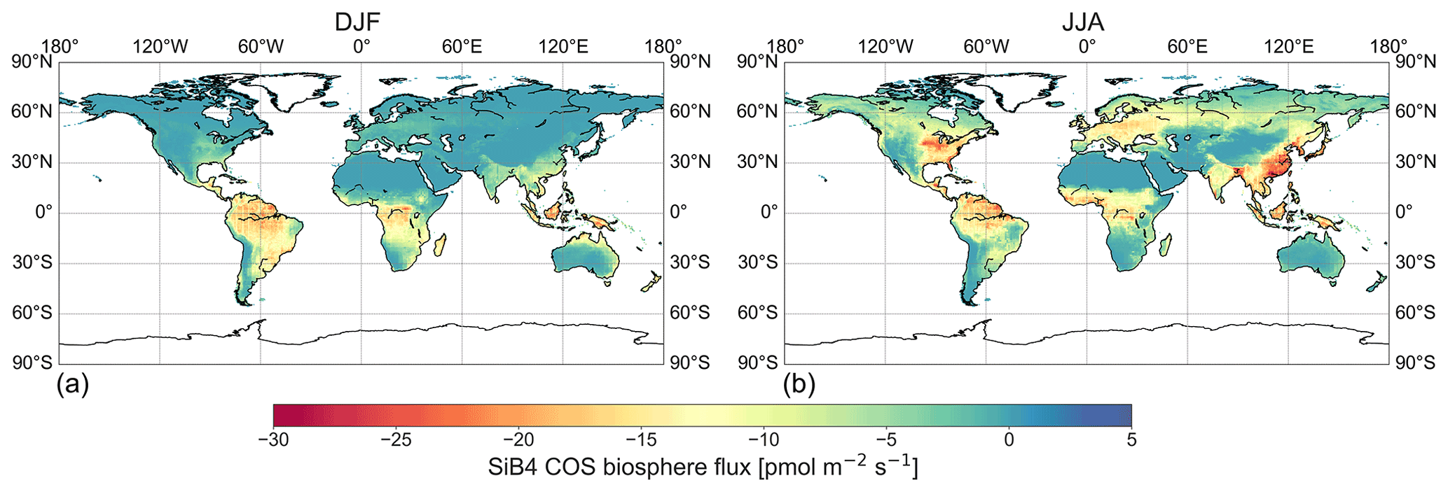
Figure 5 Global distribution of the COS biosphere flux in DJF (a) and JJA (b) as simulated by SiB4_var_Ogee over the years 2000–2020. Negative values indicate uptake of COS by the biosphere, while positive values indicate COS emissions.

Figure 6 COS biosphere flux difference between two SiB4 model runs. (a) Difference between SiB4_500_Berry and SiB4_500_Ogee to show the flux difference between the soil models. (b) Difference between SiB4_500_Ogee and SiB4_var_Ogee to show the effect of changing to variable mole fractions. Negative values indicate a drop in the biosphere COS uptake.

The largest decrease in the global COS biosphere sink (169 Gg S yr⁻¹, i.e., from 922 to 753 Gg S yr⁻¹) occurs in the tropics (113 Gg S yr⁻¹ for latitudes between −23.5 and +23.5^∘ N) as the high productivity in the tropics leads to the largest COS uptake and the largest decrease in COS mole fractions. This update is a significant contribution to closing the gap in the COS budget of ∼432 Gg S yr⁻¹ (Ma et al., 2021); however, it does not fully eliminate the missing source in the COS budget. The biosphere flux resulting from inverse modeling by Ma et al. (2021) indicates COS emissions in the Amazon (Fig. S17 in the Supplement). While biosphere emissions over the Amazon are unrealistic (Glatthor et al., 2015), it reflects the large missing source in the tropics (land and ocean) that we are unable to attribute sources to the biosphere; see a comparison of our SiB4 biosphere flux with the inverted biosphere flux by Ma et al. (2021) in Fig. S17. A potential reason for the unrealistic attribution of missing sources of COS is that there are no NOAA observations in the tropics and its upwind regions to constrain the TM5 inversions. For these reasons, it is unlikely that the gap in the COS budget is solely caused by an overestimated tropical biosphere sink. Still, flux observations in the tropics would have to confirm this.

In Sect. 3.1.3 we found on average an 8±27 % underestimation of the daytime COS vegetation flux as simulated by SiB4. If we assume that the daytime uptake dominates the total COS uptake and we correct the COS vegetation sink for the underestimation globally, then we find a vegetation sink of 717±179 Gg S yr⁻¹ instead of 664 Gg S yr⁻¹ and a total biosphere uptake of 806±179 Gg S yr⁻¹ instead of 753 Gg S yr⁻¹. Note, however, that this scaling is highly uncertain because we found substantial variability between sites, and a large fraction of the uptake occurs in the tropics, for which we cannot validate SiB4 due to a lack of observations.

4 Recommendations for COS-specific future model development

We found model–observation biases that could be ascribed to different components of the model (depending on the site), such as the soil COS flux or vegetation COS uptake, where the latter was caused by underestimated enzyme activity that also links to GPP. If sufficient COS flux observations were available, these could help as an extra constraint to improve the model enzyme activity and thereby GPP. Such an approach would require a number of advancements in the understanding and implementation of COS biosphere exchange in SiB4. We have identified a number of ways to improve the COS flux simulations in SiB4, which might also apply to mechanistic COS implementations in other biosphere models:

1. The simulation of COS uptake is strongly coupled to GPP through g_s and V_max (which is included in g_cos) and therefore relies on the accuracy of these model parameters. However, several studies have shown that the ratio of COS to CO₂ deposition velocities (in the literature also called “leaf relative uptake”) varies with temperature (Cochavi et al., 2021; Stimler et al., 2010) and humidity (Sun et al., 2018b; Kooijmans et al., 2019), in addition to the better known variability with light. The temperature response of the COS uptake is currently taken from V_max and is scaled with an empirical temperature function (Eq. 2) and an additional factor $T_{\text{can}}/T_{\mathrm{0}}$ (Eq. 3), where the latter increases the COS uptake at higher temperatures. However, the $T_{\text{can}}/T_{\mathrm{0}}$ term has been added as a simple correction but has not been empirically derived. We suggest a refined calibration of the internal conductance g_cos such that it captures the true temperature variation in COS vegetation fluxes. The temperature dependence of the CA enzyme activity could be determined from laboratory experiments to be able to keep effects other than temperature (e.g., on mesophyll conductance) constant. Field observations could then be used to scale the laboratory-based calibration to the ecosystem level and to different PFTs.

2. SiB4 is capable of simulating nighttime COS vegetation uptake through stomatal opening, although the nighttime uptake was often underestimated (Fig. 2). As nighttime COS vegetation uptake is driven by stomatal opening, COS flux observations can be used to estimate nighttime stomatal conductance (g_dark) (Berkelhammer et al., 2020; Maignan et al., 2021; Wehr et al., 2017). Assuming that g₀ is representative of g_dark, these COS-based values can be tested in SiB4. However, similar approaches and processing techniques are required to be able to evaluate the accuracy of the nighttime COS uptake and determine the nighttime stomatal conductance. Changing g₀ values in SiB4 would also have consequences for simulations of daytime carbon, water, and energy, which should also be (re-)evaluated.

3. We have seen that the simulated COS soil flux can be very different depending on the biome (in SiB4 selected as the PFT). This is especially true for fertilized soils that are typically found in agricultural sites, where large emissions of COS are observed. However, soils can contain high nitrogen contents regardless of whether or not they are agricultural soils. Therefore, it is important to know the nitrogen content for setting the soil COS uptake and production parameter values for the COS soil flux calculation (Table 2). We suggest the use of global maps of the soil nitrogen content and of the relation between COS soil production and soil nitrogen content (Kaisermann et al., 2018b) for more accurate COS soil production simulations.

4. This study relied on the availability of field observations. We were able to evaluate SiB4 with the COS field observations available from a number of PFTs. However, we lacked observations on evergreen broadleaf forests that are largely represented in the tropics. Such observations could give further insights into the COS budget in the tropics, where currently the largest uncertainties exist. Moreover, controlled laboratory measurements of soil COS exchange have been shown to be very powerful in understanding the soil COS exchange and in parameterizing COS soil models (Meredith et al., 2018, 2019). However, field observations of COS soil exchange along with ecosystem COS fluxes are needed to evaluate COS soil models under field conditions (Ogée et al., 2016; Sun et al., 2015), which would also require standardization of measurement and processing techniques (Kohonen et al., 2020). Finally, the NOAA measurement network of atmospheric COS mole fractions has good coverage over North America and the Pacific Ocean, but other regions are less well represented. The COS mole fraction fields that we prescribed to SiB4 rely on the availability of COS observations. Better global coverage of COS mole fraction observations would therefore be beneficial, e.g., through the use of satellite data, where sensitivity to the middle and upper troposphere can currently be achieved (Glatthor et al., 2015; Kuai et al., 2014). Moreover, SiB4 should ideally be directly coupled to an atmospheric transport model to account for the interconnection between COS uptake and COS mole fractions.

5 Conclusions

The experimental efforts made in the last decade to obtain field observations of COS ecosystem fluxes now offer the possibility of a unique SiB4 model validation of COS biosphere exchange over different biomes. SiB4 was capable of simulating the diurnal and seasonal variations in COS fluxes in the boreal, temperate, and Mediterranean region but with an average underestimation of 8±27 % of the daytime vegetation flux. The magnitude of the biases differed per site but could not be ascribed to a single component of the model. We found a lower global soil COS sink with the implementation of the Ogée et al. (2016) soil COS model. Still, the soil COS flux remains a relatively small component in the total COS budget, which supports the use of atmospheric COS as a global- and regional-scale photosynthesis tracer. A larger effect on the global COS biosphere sink was found by changing the fixed COS mole fraction of 500 pmol mol⁻¹ to values that vary spatially and temporally. The reduction in the COS sink strength is most pronounced in regions with large biomass such as the tropics. This analysis highlights the importance of accounting for variations in atmospheric COS mole fractions, which has not yet been adopted as standard practice. We make a number of recommendations for future improvements of the model, including re-calibration of the COS model parameters. However, we are limited by site- and leaf-level data coverage in being able to accurately constrain the model over different PFTs and seasons. More campaigns and long-term observations in underrepresented PFTs, biomes, and soil types and more laboratory measurements such as for CA sensitivity in leaves and soils would be key to continued improvement of the model.