the Creative Commons Attribution 4.0 License.
the Creative Commons Attribution 4.0 License.
 | 17 Feb 2022
Sea ice concentration impacts dissolved organic gases in the Canadian Arctic
Anna E. Jones
William T. Sturges
Philip D. Nightingale
Brent Else
Brian J. Butterworth
The marginal sea ice zone has been identified as a source of different climate-active gases to the atmosphere due to its unique biogeochemistry. However, it remains highly undersampled, and the impact of summertime changes in sea ice concentration on the distributions of these gases is poorly understood. To address this, we present measurements of dissolved methanol, acetone, acetaldehyde, dimethyl sulfide, and isoprene in the sea ice zone of the Canadian Arctic from the surface down to 60 m. The measurements were made using a segmented flow coil equilibrator coupled to a proton-transfer-reaction mass spectrometer. These gases varied in concentrations with depth, with the highest concentrations generally observed near the surface. Underway (3–4 m) measurements showed higher concentrations in partial sea ice cover compared to ice-free waters for most compounds. The large number of depth profiles at different sea ice concentrations enables the proposition of the likely dominant production processes of these compounds in this area. Methanol concentrations appear to be controlled by specific biological consumption processes. Acetone and acetaldehyde concentrations are influenced by the penetration depth of light and stratification, implying dominant photochemical sources in this area. Dimethyl sulfide and isoprene both display higher surface concentrations in partial sea ice cover compared to ice-free waters due to ice edge blooms. Differences in underway concentrations based on sampling region suggest that water masses moving away from the ice edge influences dissolved gas concentrations. Dimethyl sulfide concentrations sometimes display a subsurface maximum in ice -free conditions, while isoprene more reliably displays a subsurface maximum. Surface gas concentrations were used to estimate their air–sea fluxes. Despite obvious in situ production, we estimate that the sea ice zone is absorbing methanol and acetone from the atmosphere. In contrast, dimethyl sulfide and isoprene are consistently emitted from the ocean, with marked episodes of high emissions during ice-free conditions, suggesting that these gases are produced in ice-covered areas and emitted once the ice has melted. Our measurements show that the seawater concentrations and air–sea fluxes of these gases are clearly impacted by sea ice concentration. These novel measurements and insights will allow us to better constrain the cycling of these gases in the polar regions and their effect on the oxidative capacity and aerosol budget in the Arctic atmosphere.
- Article
(6351 KB) - Full-text XML
-
Supplement
(332 KB) - BibTeX
- EndNote


The Arctic is an important part of the global climate system and is warming faster than the rest of the world (Dai et al., 2019). One of the most obvious signs of the warming and changing Arctic is the changes in sea ice. Sea ice is rapidly decreasing in extent and concentration (Meier et al., 2014; Z. Wang et al., 2020), melting earlier, and freezing up later in the season (Markus et al., 2009; Z. Wang et al., 2020). The effects of these changes on the marine biogeochemistry and trace gas emissions are poorly known (Huntington et al., 2019; Steiner et al., 2021), largely due to a lack of measurements. Understanding these effects is particularly relevant as areas of open water and open pack ice, which are becoming more frequent features of the Arctic, have been associated with new particle formation (Collins et al., 2017; Dall'Osto et al., 2018). This suggests a possible negative feedback link between changes in sea ice and Arctic climate (Dall'Osto et al., 2017), potentially leading to reduced Arctic warming (Mahmood et al., 2018; Paasonen et al., 2013). Such a link could proceed via emission of a cocktail of trace gases from the ice-uncovered waters, leading to increased cloud condensation nuclei (Collins et al., 2017; Köllner et al., 2017; Mungall et al., 2017). Most of the new particles formed in the Canadian Arctic (Tremblay et al., 2019) and the remote ocean (Zheng et al., 2020) appear to consist of organic material and sulfate (oxidation product of dimethyl sulfide).
In this paper, we focus on the impact of sea ice concentration on the seawater concentrations and air–sea fluxes of methanol, acetone, acetaldehyde, dimethyl sulfide (DMS), and isoprene. Global ocean fluxes of methanol, acetone, acetaldehyde, and isoprene are highly uncertain (Arnold et al., 2009; Bates et al., 2021; Wang et al., 2019; S. Wang et al., 2020). Therefore these measurements will help to constrain the ocean emissions of these gases not only in the polar region but also globally.
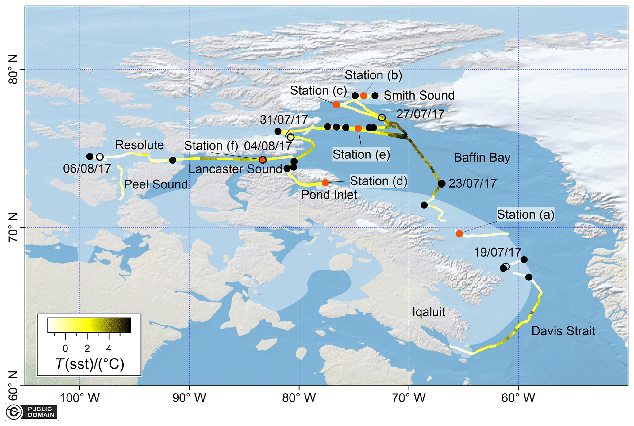
Figure 1Cruise track of the sampling undertaken in the Arctic sea ice zone coloured by sea surface temperature (SST). Sampling dates are indicated as hollow circles marked with the date. The location of each CTD station where sampling was undertaken is indicated as a closed black dot. Highlighted CTD stations are indicated as closed orange dots and labelled by station number. Interruptions in the cruise track and underway auxiliary data are due to interruptions in the ship underway logging system (Amundsen Science Data Collection, 2017). All the map data were created from public domain GIS data found on the Natural Earth website (http://www.naturalearthdata.com, last access: 15 April 2021). They were read into Igor using the Igor GIS XOP beta. The sea-ice-covered area is approximately indicated for illustration purposes as a shaded area due to the dynamic nature of sea ice and difficulties in conveying this information for a month-long deployment. The approximate location of the sea ice edge is based on the average sea ice concentration for the whole cruise duration using AMSR2 satellite data. Details on the sea ice concentration data used for analysis can be found in the text (Sect. 2.1).
All of these gases have known sources in seawater that are potentially enhanced in the marginal sea ice zone. Methanol is produced by phytoplankton (Kameyama et al., 2011; Mincer and Aicher, 2016) and consumed by microbes (Dixon et al., 2011, 2013; Sargeant et al., 2016). Acetone is thought to be produced primarily from photochemical reactions (de Bruyn et al., 2011; Dixon et al., 2013; Kieber et al., 1990) and consumed by microbes (Dixon et al., 2014). A biological source of acetone has also been suggested from culture experiments (Davie-Martin et al., 2020; Halsey et al., 2017) and correlations of field data (Schlundt et al., 2017), though it is thought to be small. Acetaldehyde is produced by photochemistry (Dixon et al., 2013; Zhu and Kieber, 2018; Kieber et al., 1990; de Bruyn et al., 2011) and in a light-dependent fashion from phytoplankton (Davie-Martin et al., 2020; Halsey et al., 2017). Acetaldehyde is consumed very rapidly by microbes, giving it a lifetime of a few hours in seawater (de Bruyn et al., 2017, 2021; Dixon et al., 2014). Acetone and methanol have highly variable lifetimes in the ocean mixed layer (5–55 d for acetone and 10–26 d for methanol; Dixon et al., 2013), with shorter lifetimes generally observed in coastal areas (de Bruyn et al., 2013; Dixon et al., 2014). Production of DMS in seawater is complex and has been the subject of many prior studies (Simó, 2001; Zhang et al., 2019). Different phytoplankton produce dimethyl sulfoniopropionate (DMSP, a key precursor for DMS) and DMS at widely different rates (Sheehan and Petrou, 2020). The largest sink of DMS in seawater is biological consumption by bacteria (Kiene and Bates, 1990; Yang et al., 2013b), giving it a turnover time between 0.5 and 2 d. Isoprene is thought to be produced by a large range of phytoplankton in the ocean (Hackenberg et al., 2017; Shaw et al., 2010) and is often parameterized with sea surface temperature and surface chlorophyll a (Chl a) concentration (Hackenberg et al., 2017; Ooki et al., 2015; Rodríguez-Ros et al., 2020). The largest sink of isoprene to the water column is thought to be air–sea exchange (Booge et al., 2018; Palmer and Shaw, 2005), giving it a lifetime of around 10 d (Booge et al., 2018).
Sea ice may directly or indirectly affect the production and consumption of these gases in seawater. In general, the water column in the high Arctic displays very shallow light penetration depths (Pavlov et al., 2015), largely due to the input of light-absorbing molecules from riverine input (Granskog et al., 2015). Seasonal sea ice meltwater input leads to deeper light penetration depths (Granskog et al., 2015). This affects the biological and photochemical production of many of the compounds discussed here. Sea ice itself is generally poorly transmissible to light, but breaks in the ice cover and melt ponds allow more light to pass, creating a very heterogenous light field (Massicotte et al., 2018). Sea ice also plays an important (but poorly understood) role in gas exchange (e.g. Butterworth and Miller 2016; Loose et al., 2014; Dong et al. 2021), which in turn would be expected to impact the source and sink terms for many of these compounds.
The Arctic Ocean and the sea ice zone represent particularly undersampled regions with no existing measurements of seawater concentrations of methanol, acetone, and acetaldehyde in partial sea ice cover. Based on atmospheric measurements and correlations with DMS, the Canadian Arctic sea ice zone is suspected to be a sink for methanol and acetone (Sjostedt et al., 2012) and a source for other oxygenated volatile organic compounds (VOCs) produced in the sea surface microlayer from photochemical activity (Mungall et al., 2017, 2018). Atmospheric measurements in eastern Greenland find that the correlation between DMS and acetone air mixing ratios changes depending on the season (Pernov et al., 2021), pointing towards seasonal changes in seawater biogeochemistry affecting emissions of these gases.
In this paper, we present depth profile (0–60 m) and underway (∼5 m) seawater measurements of methanol, acetone, acetaldehyde, DMS, and isoprene in the Canadian Arctic during boreal summer (July–August 2017). Importantly, these data enable assessment of the air–sea fluxes of these gases. Combining these measurements, we investigate the impact of sea ice concentration on the dissolved concentrations of these VOCs.
2.1 Description of the cruise sampling
Depth profile and underway measurements of dissolved gas concentrations in the sea ice zone of the Canadian Arctic were measured on board the icebreaker CCGS Amundsen. The measurements were taken between 17 July and 8 August 2017 (Cruise 1702, leg 2b) (Fig. 1).

Figure 2Overview plot displaying the shape of all methanol and density (σT) depth profiles, grouped by SIC and staggered along the x axis for ease of viewing. Panel labels indicate the SIC bin. The scale bars for methanol and density in (a) also apply to (b) and (c). Profiles with hollow markers are highlighted in Fig. 7. Sampling dates are indicated to locate stations using Fig. 1. Panels (d) to (f) indicate absolute concentrations of mean vertical profiles grouped according to ice cover and binned by depth horizons. The shaded area indicates standard error for each depth horizon.
The research vessel travelled from Iqaluit northwards through Davis Strait and western Baffin Bay to reach Smith Sound. In this area, more intense depth profile sampling was carried out. The vessel then travelled to Pond Inlet and Resolute via Lancaster Sound. Sampling ended south of Resolute in Peel Sound.
The general hydrography of the Canadian Arctic is very well described by McLaughlin et al. (2004). Briefly, Pacific and Arctic waters flow westwards through the narrow channels of the Canadian Arctic into Baffin Bay and the North Atlantic (McLaughlin et al., 2004), with the fastest flows observed in summer (Prinsenberg and Hamilton, 2005). Most of this surface water flow occurs through the largest channels, namely Lancaster Sound and Smith Sound (Melling et al., 2001). At the same time, recurrent ice bridges tend to form across Lancaster sound and north of Smith Sound, which lead to ice-free areas (polynyas) (McLaughlin et al., 2004). Once in Baffin Bay, these Pacific and Arctic water masses flow southwest along the east coast (Burgers et al., 2020; McLaughlin et al., 2004) of Baffin Island.
Depth profiles of dissolved gas concentrations were measured from the Rosette-mounted Niskin bottles as discrete samples from near the surface (about 2 m) to 60 m depth at a total of 21 stations as per availability. A range of sensors were mounted on the Rosette frame to measure biogeochemical variables from 2 m downwards, such as oxygen concentration (monitored using a Seabird 43), conductivity (Seabird 4), Chl a (Sea point Chlorophyll Fluorometer), PAR irradiance (QCP-2300 Biospherical), temperature (Seabird 3 plus), and pressure (Paroscientific Digiquartz). Inorganic nutrient measurements (nitrate) were carried out as described in Randelhoff et al. (2019).
When logistically feasible at a station, a handheld vertical 5 dm3 Niskin bottle was deployed off the front starboard side of the ship to sample approximately the top 30 cm from the ocean surface. This was done by bringing the Niskin bottle up from approximately 3 m and firing it just before it reached the surface using rope marks as depth indicators, similar to the method described in Ahmed et al. (2020). Samples collected with this method are marked in the data presentation. This sampling was preceded by the deployment of a handheld conductivity–temperature–depth (CTD) logger (RBR XR-420) to characterize the salinity and temperature in the upper metres of the ocean. Data from this logger is presented at 0.5 m resolution for the 2 m near the surface.
A range of biogeochemical parameters were monitored continuously underway, including sea surface temperature (SST) (Sea Bird SBE 38), sea surface salinity (SSS) (Sea Bird SBE 45 MicroTSG Thermosalinograph), and Chl a fluorescence (Wetlabs WETStar Fluorometer). When not used for discrete sampling, the VOC measurement system (see the next section) was also used for continuous sampling of the underway water.
Wind speed was measured from a meteorological tower (approximately 16 m a.s.l) located on the foredeck of the ship, similar to that described in Ahmed et al. (2019). The measured wind speeds at 16 m a.s.l. were converted to 10 m wind speed (U10) based on a logarithmic wind profile (Kaimal and Finnigan, 1994) and corrected for speed of ship passage.
The AMSR2 passive microwave sea ice concentration (SIC) satellite product (daily, 3125 km × 3125 km resolution) (Spreen et al., 2008) was used to create a time series of sea ice concentration along the cruise track. This product is chosen due to its high spatial and temporal resolution and its complete coverage of the cruise track. From each daily satellite image, the sea ice concentration of the grid cell where the ship was located during that hour was extracted. The sea ice cruise track time series deduced from the AMSR2 satellite product and visual ship-based ice fraction observations largely agree and show no major systematic bias (Sect. S1). Due to its wider spatial coverage, the satellite time series is used to infer the impact of seasonal sea ice melt on the underway dissolved concentrations of VOCs. Visual SIC observations were made during CTD casts directly from the CTD launch point on deck, and thus those estimates were used to interpret vertical profile measurements.
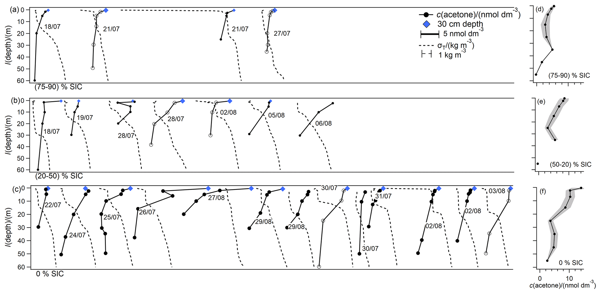
Figure 3Overview plot displaying the shape of all acetone and density (σT) depth profiles, grouped by SIC and staggered along the x axis for ease of viewing. Panel labels indicate the SIC bin. The scale bars for acetone and density in (a) also apply to (b) and (c). Profiles with hollow markers are highlighted in Fig. 7. Sampling dates are indicated to locate stations using Fig. 1. Panels (d) to (f) indicate absolute concentrations of mean vertical profiles grouped according to ice cover and binned by depth horizons. The shaded area indicates standard error for each depth horizon.
In the analysis below, we mainly assess how the depth profiles and underway seawater VOC concentrations vary with SIC. From this, the impact of seasonal sea ice melt on VOC cycling is inferred.
2.2 Dissolved gas measurements
A segmented flow coil equilibrator (SFCE) coupled to a proton-transfer-reaction mass spectrometer (PTR-MS) was used to measure dissolved gases in seawater (Wohl et al., 2019). The SFCE–PTR-MS system was set up in one of the labs located near the front of the ship with access to an underway water tap from the ship's main underway water supply (located at 3–4 m depth). Discrete water samples (for depth profiles) were taken from the Niskin bottles in a gas-sensitive fashion into 900 cm3 glass bottles with glass caps. For discrete VOC measurements, the SFCE sampled from the bottom of these glass bottles. At a water flow rate of about 100 cm3 min−1, this water volume was enough for a stable measurement (i.e. average of ∼6 min), where the top 5 cm of water in the glass bottle was not sampled due to possible atmospheric contamination. For underway measurements, the SFCE sampled from the bottom of a glass bottle in the sink, which was rapidly overflowed with the ship's underway water. During periods of high sea ice cover, as per decision by the ship's crew, the underway water inlet was turned off. The underway water flow rate was continuously monitored by the ship's crew and used for data quality control. For more information on the on-board installation and a comparison of CTD to underway measurements, please refer to Wohl et al. (2019).
The computation of dissolved gas concentrations specific to this deployment is laid out in Sect. S2. Comparisons between near-surface CTD and underway measurements suggested an initial acetaldehyde contamination in the CTD rosette bottles due to the use of an air duster aerosol spray used near the rosette. The other VOCs were not affected. After use of the spray was stopped on 26 July 2017, the acetaldehyde contamination in the CTD measurements immediately disappeared. Thus, acetaldehyde CTD measurements collected prior to 26 July 2017 are not included in this analysis.
3.1 Depth profile distributions
To illustrate the effect of SIC on the depth profile distributions of these dissolved gases, we first focus on the shape of their depth profiles. A discussion of the effect of sea ice on the absolute dissolved gas concentrations follows, which predominantly considers the underway measurements leading to a much greater sample size.

Figure 4Overview plot displaying the shape of all acetaldehyde and density (σT) depth profiles, grouped by SIC and staggered along the x axis for ease of viewing. Panel labels indicate the SIC bin. The scale bars for acetaldehyde and density in (a) also apply to (b) and (c). Profiles with hollow markers are highlighted in Fig. 7. Sampling dates are indicated to locate stations using Fig. 1. Panels (d) to (f) indicate absolute concentrations of mean vertical profiles grouped according to ice cover and binned by depth horizons. The shaded area indicates standard error for each depth horizon (acetal. is short for acetaldehyde).
Figures 2 to 6 are overview plots that focus on the VOC depth profile shapes and corresponding auxiliary data. The casts have been grouped in panels by SIC (indicated at the bottom of the panel). The grouping is based on the following definitions: in remote sensing, an ice-free area is generally considered to display ice coverage of less than 15 % (Z. Wang et al., 2020), and ice breakup has been defined by Ahmed et al. (2019) as the time the sea ice concentration changes from above to below 90 %. Based on these few definitions, sampled stations and corresponding SIC stations were grouped as (i) 75 %–90 % near full ice cover or during ice break up, (ii) 50 %–20 % partial sea ice coverage, or (iii) 0 %–15 % ice-free. No stations were sampled with SIC 75 %–50 %.
The overview plots (panels a–c in Figs. 2 to 6) are staggered along the x axis by sampling order for ease of viewing. The sequence of the casts is the same for all compounds except acetaldehyde (due to missing depth profile data). Sampling dates are indicated next to the cast shape. Scale bars for VOC concentrations and auxiliary data are also included.
Panels d and e in Figs 2 to 6 indicate mean vertical profiles grouped according to ice cover and binned in different depth horizons. These mean vertical profiles show mean absolute concentrations at different depths for a range of sea ice concentrations. Binning depth horizons were as follows: 0–0.5, 0.5–4, 4–10, 10–20, 20–30, 30–40, 40–50, and 50–60 m. Smaller bins were chosen near the surface to investigate the near surface gradients.
Additionally, six casts are highlighted in a separate figure, along with more detailed auxiliary data, to show absolute concentrations and allow comparisons between casts (Fig. 7). These profiles are chosen from careful examinations of the overview plots as they (i) represent the typical effect of sea ice on these compounds, (ii) present higher vertical resolution near the surface, and (iii) contain acetaldehyde concentrations that could not be determined for all profiles. The highlighted casts are also marked in the overview plots. Seawater samples collected with a handheld Niskin from about 30 cm depth are marked as a blue diamond. Density, calculated from temperature and salinity data, for the surface 2 m is only presented when near-surface sampling was carried out.
Here we briefly discuss the effect of sea ice concentration on water column structure and biogeochemistry to provide context for the dissolved gas measurements. As shown in Fig. 7 and Fig. 2 for example, the stations with near full ice cover or that are during ice break up (75 % to 90 % SIC, following the definition of ice breakup by Ahmed et al., 2019) show fairly small density and salinity gradients between 2 and 60 m depth, perhaps due to limited wind-driven mixing. In these casts, high concentrations of Chl a were found at 2 m, and Chl a concentrations then gradually decreased down to 60 m (Figs. 5 and 7).
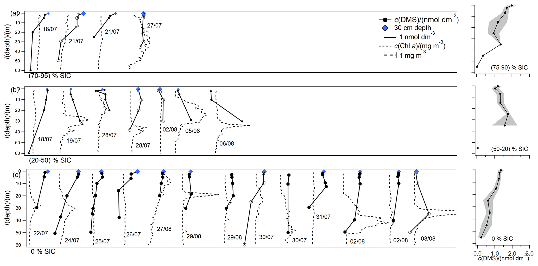
Figure 5Overview plot displaying the shape of all DMS and Chl a depth profiles, grouped by SIC and staggered along the x axis for ease of viewing. Panel labels indicate the SIC bin. The scale bars for DMS and Chl a in (a) also apply to (b) and (c). Profiles with hollow markers are highlighted in Fig. 7. One of the Chl a profiles is cut off in (c) for scale purposes. Sampling dates are indicated to locate stations using Fig. 1. Panels (d) to (f) indicate absolute concentrations of mean vertical profiles grouped according to ice cover and binned by depth horizons. The shaded area indicates standard error for each depth horizon.
Stations with lower ice coverage (20 % to 50 % SIC) tend to display a more defined, very shallow mixed layer of similar density and salinity between 2 and ca. 10 m. A deep Chl a maximum is observed just below the density gradient (at ca. 10 m depth, Fig. 7), similar to previous observations (Martin et al., 2010; Randelhoff et al., 2019). This deep Chl a maximum at some of the stations (Fig. 7) could be characterized by very high levels of biological activity (Ardyna et al., 2013; Barber et al., 2015; Burgers et al., 2020).
Ice-free casts (0 % SIC) display a deeper (from 2 to ca. 20 m depth) and warmer mixed layer of similar density and salinity (Fig. 7) – useful indicators for how long these stations have been free of ice (Randelhoff et al., 2019; Shadwick et al., 2013). The density gradient at the base of this mixed layer is much larger at these ice-free stations, and many of the profiles display a very pronounced deep Chl a maximum just below the mixed layer, while surface Chl a is generally lower (Fig. 7). Even ice-free areas display very low salinities (between 32 and 28, Fig. 7), which is typical for the Canadian Arctic Archipelago (McLaughlin et al., 2004) and indicates that the waters sampled here are heavily influenced by sea ice melt and riverine discharge.
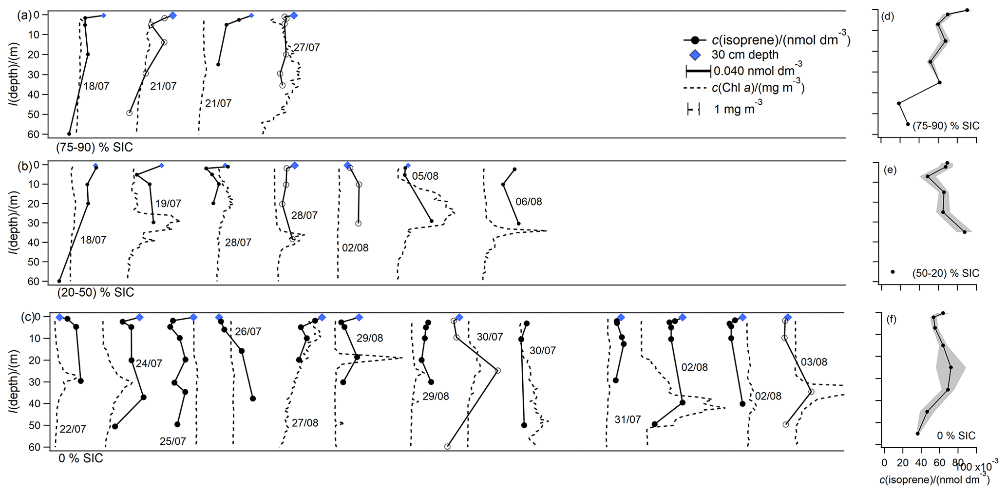
Figure 6Overview plot displaying the shape of all isoprene and Chl a depth profiles, grouped by SIC and staggered along the x axis for ease of viewing. Panel labels indicate the SIC bin. The scale bars for isoprene and Chl a in (a) also apply to (b) and (c). Profiles with hollow markers are highlighted in Fig. 7. One of the Chl a profiles is cut off in (c) for scale purposes. Sampling dates are indicated to locate stations using Fig. 1. Panels (d) to (f) indicate absolute concentrations of mean vertical profiles grouped according to ice cover and binned by depth horizons. The shaded area indicates standard error for each depth horizon.
All casts display very low nitrate concentrations at the surface (<1 µmol dm−3), which rapidly increase near the mixed-layer depth. This suggests that, in general, the spring phytoplankton bloom sampled here is in an advanced stage as nutrients near the surface are depleted (Randelhoff et al., 2019).
Salinity and density measurements between the surface and 2 m show that about half of the casts display lower-density waters in the top 1 m (e.g. Fig. 2) coinciding with lower salinity and sometimes higher temperature (Fig. 7). In the data shown here, this surface stratified layer tended to be more common in casts with partial sea ice cover but also occurred when no sea ice was present at the time of sampling (Figs. 7 and 2). We speculate that this surface stratified layer is largely due to sea ice melt in the Canadian Arctic Archipelago (Ahmed et al., 2020; Burt et al., 2016; Miller et al., 2019).
We next present the underway measurements of these gases. Combining the depth profiles with the underway measurements, we discuss how the seawater concentrations of the trace gases change with different SIC in Sect. 4.

Figure 7Depth profile concentrations arranged by decreasing SIC. Geographical locations of the stations in panels (a) to (f) are indicated in Fig. 1. SIC at the time of sampling was (a) 90 %, (b) 75 %, (c) 50 %, ((d) 20 %, (e) 0 %, and (f) 0 %, where 0 % indicates ice free at the time of sampling (acetal. is short for acetaldehyde; temp. is short for temperature); ∗ Chl a increases up to 13 mg dm−3 at the Chl a maximum (Amundsen Science Data Collection, 2017). Error bars show measurement noise. Limited measurements of acetaldehyde during the early part of the cruise are due to contamination from the CTD, and the single measurement came from the handheld Niskin bottle (30 cm depth).
3.2 Underway measurements
Compared to CTD measurements at stations, the underway measurements presented in this section have a much higher temporal and spatial coverage. Hence, they can be used to derive more robust statistics and investigate the effect of sea ice on absolute concentrations in surface seawater. These underway measurements are compared to previous observations in other parts of the ocean and are also used to derive correlations with ancillary measurements.
Underway seawater concentrations of methanol, acetone, acetaldehyde and isoprene are presented in Fig. 8 along with the concentrations measured from the 5 m Niskin bottle. Underway SST, SIC, Chl a, and SSS are also presented.
The underway time series (Fig. 8) shows generally higher Chl a surface concentrations in partial ice cover compared to ice-free or full ice cover areas. These may be in part due to ice-edge blooms, which are frequent features of the Arctic sea ice zone (Barber et al., 2015; Levasseur, 2013; Perrette et al., 2011; Randelhoff et al., 2019). Nitrate concentrations at 5 m ranged between 0 and 0.7 µmol dm−3 suggesting that the phytoplankton bloom sampled here is very advanced.
To further investigate the effect of sea ice on surface seawater concentrations of the compounds measured in this study, the measured concentrations are plotted against sea ice concentration at the time of sampling and bin averaged to 10 % SIC bins (Fig. 9). A total of 61 hourly underway surface seawater measurements were taken in partial ice cover, which represents 23 % of the underway measurements shown here.
To investigate the effect of sea ice edges and water mass circulation on the surface concentrations of these compounds, we calculate mean underway surface concentrations measured in different sampling areas: western Baffin Bay (17–23 July), Smith Sound (23–31 July), and Lancaster Sound (31 July–7 August). These areas were chosen as they divide the cruise track in three equally representable sections and allow us to comment on the effect of water circulation relative to sea ice edges and ice bridges. Means and standard errors of dissolved gas concentrations and some auxiliary data are presented in Sect. S3. Sea ice bridges are often observed north of Smith Sound and east of Lancaster Sound (Lizotte et al., 2020; McLaughlin et al., 2004). At the same time, surface waters flow southwards and westwards from these sea ice bridges (McLaughlin et al., 2004; Münchow et al., 2015). This makes Smith Sound and Lancaster Sound ideal locations to sample downstream of an ice edge.
The depth profiles and underway data discussed in the following section represent measurements at different times and locations. Therefore, differences are possibly due not only to sea ice coverage but also the oceanography of the area (McLaughlin et al., 2004). We recognize that sea ice is a very heterogenous environment with respect to ice thickness (Hayashida et al., 2020), the presence of melt ponds (Gourdal et al., 2018; Park et al., 2019), and types of sea ice (e.g. first year vs. multi-year ice, Lizotte et al., 2020). This heterogeneity likely leads to very different biogeochemistry, affecting trace gas cycling. Most of the discussion that follows here focusses largely on the effect of sea ice concentration on these gases and does not always explicitly take into consideration the effect of these variables, which is worthy of future research.
Additionally, we speculate in this section about the dominant processes (photochemistry or biological source or sink) based on variations in concentrations. This speculation could have been more conclusive if we had made concurrent rate measurements.
4.1 Methanol
Casts with near full ice cover (75 % to 90 % SIC) displayed somewhat similar concentrations of methanol throughout the top 60 m (Fig. 2a, d), while partially ice-covered (20 % to 50 % SIC) and ice-free casts displayed higher methanol concentrations in the mixed layer and near the surface (Fig. 2b, e, c, f). Many of the ice-free casts that display lower-density seawater near the surface also tended to show higher methanol concentrations at 30 cm (Fig. 2c, f). The few methanol profiles collected in the temperate and tropical Atlantic generally indicate higher concentrations of methanol within the mixed layer than below (Beale et al., 2013; Williams et al., 2004; Yang et al., 2014b). Higher methanol concentrations near the surface could be due to air to sea deposition of methanol in ice-free conditions. In seawater, methanol is produced by a large range of phytoplankton (Davie-Martin et al., 2020; Mincer and Aicher, 2016) and consumed by bacteria (Dixon and Nightingale, 2012; Sargeant et al., 2016). Higher concentrations near the surface at stations of low ice coverage appear to be consistent with a biological source of methanol in seawater, as ice-free areas typically display higher net community production (Burgers et al., 2020), and most primary productivity tends to occur within the 30 m near the surface (Arrigo et al., 2011). We observe no obvious relationship between methanol concentration and Chl a in this dataset. This might be because the balance between biological production and consumption depends on the phytoplankton and bacteria species present (Mincer and Aicher, 2016; Sargeant et al., 2016). Methanol concentrations near the surface tend to be quite variable, which could be because biological consumption rates are also highly variable with depth (Dixon and Nightingale, 2012). Indeed, some ice-free casts display higher methanol concentration in the top 2 m and 30 cm compared to the rest of the mixed layer (Figs. 2c, f, 7).The shapes of the methanol depth profiles are remarkably similar to other compounds that display photochemical sources (acetone, acetaldehyde), which suggests a possible role of light in methanol production. Since the presence or absence of sea ice is a major control on the amount of light in the upper ocean, our observations of higher methanol at lower sea ice concentration also suggests a light-dependent source. Previous experiments suggest that direct photochemical production of methanol is negligible (Dixon et al., 2013). Higher light intensity has been shown to lead to higher biological methanol production rates (Halsey et al., 2017). However, those experiments used visible light, which penetrates deeper into the water column (≈40–50 m; Massicotte et al., 2018; Fig. 7). The near-surface enhancement in methanol we observed here suggests that this methanol concentration gradient may be caused by ultraviolet (UV) light, which penetrates to around 2–7 m (Tedetti and Semperv, 2006). We speculate that the very near-surface enhancement in methanol concentrations (within the top ≈2 m) could have been due in part to cell lysis caused by damaging UV light. Cell lysis has been suspected to possibly interfere with previous methanol production rate measurements (Davie-Martin et al., 2020). Lethal levels of UV light have been observed to depths of 2–3 m in the Arctic (Tedetti and Semperv, 2006).
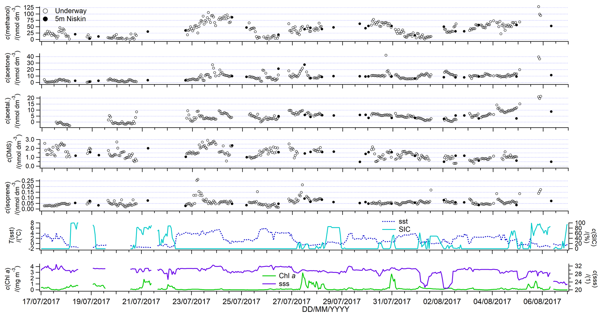
Figure 8Underway surface water concentrations of dissolved gases. Plotted along are underway SIC, SST, Chl a, and salinity (Amundsen Science Data Collection, 2017).
The mean underway surface seawater concentration of methanol was 38 nmol dm−3, and the median was 36 nmol dm−3. This is within the range of previous seawater measurements (Beale et al., 2013; Kameyama et al., 2010; Williams et al., 2004), and the mean is similar to measurements at UK shelf seas (Beale et al., 2015) and in the temperate Atlantic (Yang et al., 2013a). Our mean concentration is about twice as high as previous measurements in the Labrador Sea in October (Yang et al., 2014a), possibly due to higher seasonal biological activity during the cruise presented here (e.g. Davie-Martin et al., 2020). Another reason for higher methanol concentrations during this cruise could be slower bacterial consumption, which has been shown to vary seasonally (Sargeant et al., 2016).
Methanol concentrations displayed a large range in concentrations (below the limit of detection up to 129 nmol dm−3), which were better resolved relative to previous discrete measurements due to the use of high-resolution underway sampling. This suggests that methanol production and consumption processes are not always tightly coupled and are instead governed by specific processes in different locations. Instead of being controlled by widespread sources, such as production by a large range of phytoplankton species (Mincer and Aicher, 2016), it is possible that methanol concentrations in the sea ice zone are heavily influenced by oxidation rates. Methanol oxidation rates tend to be highly variable (Dixon et al., 2011; Dixon and Nightingale, 2012) and influenced by the microbial species present (Sargeant et al., 2016, 2018). Methanol oxidation rates have also been shown to influence seawater methanol concentrations in coastal waters (Beale et al., 2015). Underway methanol concentrations do not appear to vary with SIC alone (Fig. 9). The presence or absence of sea ice at the time of sampling appears to influence methanol concentrations more strongly. This is further supported by the fact that higher methanol seawater concentrations were measured in the relatively ice-free Smith Sound (46 nmol dm−3) and Lancaster Sound (41 nmol dm−3), compared to the more ice-covered region of western Baffin Bay (23 nmol dm−3). Our underway methanol measurements support dominant biological cycling of methanol, while oxidation rates probably exert a strong influence on dissolved concentrations.
4.2 Acetone
The stations with the highest SIC (75 % to 90 %) displayed the highest concentrations at the surface, which decreased rapidly with depth and reached a near-constant value at around 5 m (Fig. 3a, d). At stations with lower ice coverage (20 % to 50 %) (Fig. 3b, e), acetone concentrations were also elevated at the surface and decreased with depth, reaching a near constant value at around 20–30 m. At some ice-free stations with a well-defined mixed layer, the concentrations of acetone in the mixed layer were very homogenous and higher than below the mixed layer (Figs. 3c, f, 7). Most of the casts that display stratification within the 2 m near the surface also display higher acetone concentrations at 30 cm compared to at 2 or 5 m. The acetone profiles could be explained by dominant photochemical production of acetone (de Bruyn et al., 2011; Dixon et al., 2013) and the penetration depth of light, which is influenced by sea ice concentration and freshwater input (Randelhoff et al., 2019). UV light is required for the photochemical production of acetone, and UV light is rapidly absorbed within the first 2–7 m of the Arctic water column (Tedetti and Semperv, 2006). Thus, the photochemical production rate is likely higher in the first 2–7 m, leading to higher concentrations of acetone near the surface. The fine-scale vertical gradients of acetone at the ice-covered stations and in the 2 m near the surface are probably preserved due small differences in density preventing mixing between the different depths. At lower sea ice concentration, sea ice meltwater leads to stratification and dilutes light-absorbing molecules, leading to deeper light penetration depths (Granskog et al., 2015; Randelhoff et al., 2019). The surface stratified layer receives most of this radiation (Granskog et al., 2015), leading to small-scale concentration gradients of acetone with the highest concentrations being at the surface. As a more defined mixed layer forms and the sea ice concentration decreases, UV light can penetrate even deeper into the water column and leads to production of acetone at deeper depths. In some of the ice-free casts, acetone is likely produced at the surface and mixed deeper, forming a fairly homogeneous profile within the mixed layer. The ice-free casts with homogeneous acetone concentrations in the mixed layer are similar to previous measurements in the open ocean (Beale et al., 2013; Williams et al., 2004). We do not observe an obvious relationship between acetone and Chl a in these depth profiles. If light-dependent biological production of acetone were an important process in the sea ice zone, we would have expected to detect substantial acetone concentrations near depths of peak Chl a and down to the penetration depth of visible light (≈20–50 m, Massicotte et al., 2018; Randelhoff et al., 2019, Fig. 7) required for biological activity. In the Baffin Bay area, potentially up to 70 % of the primary productivity is occurring at the deep Chl a maximum (Burgers et al., 2020). Earlier incubation experiments suggest that biological production of acetone is negligible (Dixon et al., 2013), while more recent field campaigns (Schlundt et al., 2017) and culture experiments (Halsey et al., 2017) suggest that acetone may have a considerable biological source. While it is possible that some of the acetone we observed below ≈10 m is derived from biological activity, the near-surface gradient of acetone concentration suggests that photochemistry is the dominant source of acetone in the upper 10 m.
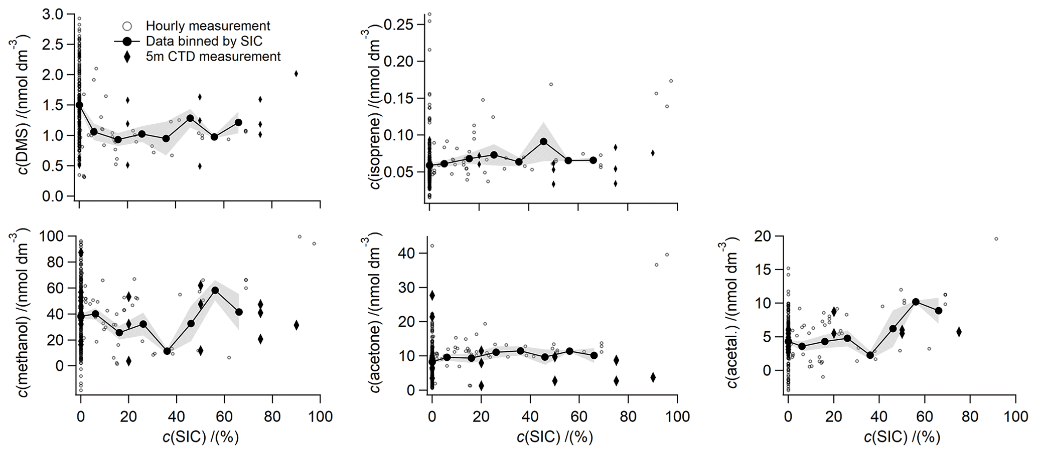
Figure 9Underway seawater concentrations plotted against SIC and binned to 10 % SIC bins. The standard error of the SIC bin is indicated as a grey-shaded area. SIC bins have only been calculated for SIC up to 70 % due to the scarcity of data at higher SIC.
The mean (median) underway seawater acetone concentration measured during this deployment is 8.9 (9.1) nmol dm−3 with a large range of 0.3 to 46.7 nmol dm−3 (Fig. 8). The mean concentration is similar to previous measurements in UK coastal waters (Beale et al., 2015) and to previous high-latitude measurements in the Labrador Sea in October (Yang et al., 2014a) and the Fram Straight in June and July (Hudson et al., 2007). Concentrations from this deployment are generally lower than other temperate and tropical open-ocean measurements (Beale et al., 2013; Kameyama et al., 2010; Marandino et al., 2005; Schlundt et al., 2017; Williams et al., 2004; Yang et al., 2014b). Acetone surface seawater concentrations have been shown to vary seasonally at a temperate site (highest concentrations in summer (Beale et al., 2015), possibly due to greater photochemical production and slower consumption during the warmer months (Dixon et al., 2014). Using a machine learning technique, S. Wang et al. (2020) also predicted the highest concentrations of acetone in the Arctic in June, July, and August of around 8–12 nmol dm−3, which is in agreement with our measurements. The episodes with the highest acetone concentrations tended to be observed during very brief periods (1–3 h) and near land during the latter part of the cruise.
Acetone displays slightly higher mean concentrations in sea-ice-covered waters (10.9 nmol dm−3) compared to ice-free waters (8.3 nmol dm−3) (t test, n1=202; n2=61; t stat = 2.5; t critical = 1.6; p=0.01) (Fig. 9). Higher concentrations of acetone in partially sea-ice-covered ocean could be due to exposure of photolabile organic carbon from under the sea ice and the influence of sea ice on light penetration depth, thus further supporting a dominant photochemical source of acetone during this cruise track. In support of this, we observe the higher mean concentrations of acetone in Smith Sound (10.8 nmol dm−3) and Lancaster sound (11.7 nmol dm−3), which are both relatively open water areas downstream of sea ice edges, compared to western Baffin Bay (3.4 nmol dm−3).
4.3 Acetaldehyde
Most acetaldehyde depth profiles display a rapid decline in concentration from the surface to about 20 m, where it reaches a value nearly constant with depth (Figs. 4, 7). Many of the casts display higher concentrations of acetaldehyde at 30 cm compared to at 2 m, especially when those depths display different densities (Fig. 4). We note that the absolute acetaldehyde concentrations presented here are uncertain due to an unquantified interference of CO2 with the background of acetaldehyde (Sect. S2). The amount of CO2 within the 60 m near the surface is not expected to vary drastically (Beaupré-Laperrière et al., 2020) and should thus not impact the shape of the acetaldehyde depth profiles, which are of value. Sharing some similarity to the acetone depth profiles, the rapid decline of acetaldehyde concentrations from the surface likely suggests a dominant light-dependent source near the surface of the water column, which is supported by previous studies (Dixon et al., 2013; Mopper and Stahovec, 1986; Zhou and Mopper, 1997; Zhu and Kieber, 2019). In contrast to acetone, acetaldehyde almost never shows a homogenous profile within the mixed layer of ice-free casts. This may be because acetaldehyde lifetime in seawater is too short (a few hours, Dixon et al., 2013) to be mixed homogenously, in contrast to acetone with its longer lifetime in seawater (5 to 55 d, Dixon et al., 2013). These profiles from the sea ice zone are in contrast to previous measurements in the open ocean of the Atlantic, where generally similar concentrations of acetaldehyde are observed at the surface compared to below the mixed layer (Beale et al., 2013; Yang et al., 2014b). These Arctic profiles compare best to depth profiles nearer to land (Beale et al., 2015; Kieber et al., 1990; Zhu and Kieber, 2019), which also show a rapid decline in concentration with depth, likely due to rapid light attenuation (Zhu and Kieber, 2019). This suggests that light penetration depth strongly influences the shape of acetaldehyde depth profiles. In the Arctic, light penetration depth is largely governed by freshwater input from melting sea ice and riverine input (Massicotte et al., 2018; Randelhoff et al., 2019). In seawater, it is thought that 7 %–53 % (Zhu and Kieber, 2019) or 16 %–68 % (Dixon et al., 2013) of acetaldehyde is produced from photochemical activity. The remainder is likely produced in a light-dependent manner from biological activity (Davie-Martin et al., 2020; Halsey et al., 2017). As mentioned previously, the wavelengths of visible light required to produce acetaldehyde from biological activity penetrate to ≈20–50 m (Massicotte et al., 2018; Randelhoff et al., 2019) (Fig. 7), while the wavelengths responsible for photochemical production are expected to penetrate only to 2–7 m (Tedetti and Semperv, 2006). Indeed, Zhu and Kieber (2019) model that about 90 % of the acetaldehyde photochemical production occurs within the upper 4 and 23 m in coastal and open-ocean waters, respectively. Thus, it is likely that some of the acetaldehyde below the penetration depth of UV light is produced from biological activity. Crucially, photochemical production, rather than biological production, appears to control the amount of acetaldehyde at the surface and thus available for air–sea exchange. We might expect a peak in acetaldehyde concentration at the deep Chl a maximum if biological production was dominant, even if it only receives 3 %–10 % of the surface irradiance (Martin et al., 2010). Our observations generally show lower concentrations below 30 m, suggesting that the main source of acetaldehyde in this area is probably photochemistry, rather than biological production. Additionally, the acetaldehyde casts from this deployment show remarkable consistency in profile shape, while Chl a (as an indicator for biological activity) was highly variable. This further supports that photochemical production in this area may be the dominant production process of acetaldehyde.
Mean (median) seawater acetaldehyde concentration was 3.7 (3.9) nmol dm−3 (Fig. 8). We reiterate that the acetaldehyde concentration measurement is possibly biased due to uncertainty in the background value. Nevertheless, this mean concentration in the Arctic compares well with open-ocean concentrations from the Atlantic (Beale et al., 2013; Yang et al., 2014b; Zhu and Kieber, 2019) and the Pacific (Kameyama et al., 2010), as well as measurements in shelf areas (Beale et al., 2015; Schlundt et al., 2017; Zhou and Mopper, 1997). There are episodes of remarkably high acetaldehyde concentrations (around 10 nmol dm−3) during this cruise track. High biological (Burgers et al., 2020) and photochemical activity (Mungall et al., 2017; Ratte et al., 1998) combined with 24 h daylight might have led to strong production of acetaldehyde during some periods of our study.
Excluding data at SIC = 0, underway acetaldehyde displays a positive correlation with SIC, with an R2 value of 0.29 (Fig. 9). Higher concentrations of acetaldehyde in partially sea-ice-covered ocean could be due to exposure of photolabile organic carbon from under the sea ice. The Arctic summertime is a hotspot for photochemical production of organic compounds (Mungall et al., 2017; Ratte et al., 1998). The origin of organic carbon has previously been shown to strongly influence the production rate of these compounds (de Bruyn et al., 2011), with unbleached, terrestrial organic carbon appearing to be a more effective precursor (Zhu and Kieber, 2018) and thus dominant in this sampling area (Mungall et al., 2017). Similarly, we observe higher concentrations of acetaldehyde in Smith Sound (5.5 nmol dm−3) and Lancaster Sound (6.0 nmol dm−3), compared to western Baffin Bay (1.1 nmol dm−3). Smith Sound and Lancaster Sound are both areas where unbleached organic carbon is exposed to light as it is moved by ocean currents from ice-covered waters into ice-free waters. This leads to higher production of acetaldehyde in these areas.
4.4 Relationships between oxygenated VOCs
In this dataset, the oxygenated VOCs correlate linearly with each other in the underway data, i.e. acetaldehyde and acetone (R2=0.35; P<0.001; N=247), acetaldehyde and methanol (R2=0.34; P<0.001; N=248), and methanol and acetone (R2=0.32; P<0.001; N=262). These correlations suggest common sources of these compounds over this cruise track, but their predictive qualities are poor, as demonstrated by low R2 values. Yang et al. (2014b) observed similar correlations during a transatlantic transect with R2 values of 0.29 (acetaldehyde vs. acetone) and 0.25 (acetaldehyde vs. methanol). However, they did not observe a correlation between methanol and acetone during their deployment. Likewise, Schlundt et al. (2017) observed correlations between acetone and acetaldehyde surface seawater with R2 values around 0.5 in the South China Sea and Sulu Sea. The correlation between acetone and acetaldehyde is likely due to common photochemical sources in this area. Similarly, acetaldehyde and acetone correlate with methanol, likely due to common light-dependent sources.
All three oxygenated VOCs measured during this cruise (methanol, acetone, and acetaldehyde) generally display lower concentrations during the first week of sampling, which corresponds to sampling the sea ice zone of the more marine-influenced western Baffin Bay area. The slightly higher concentrations of these compounds nearer to land, i.e. in Smith Sound and Lancaster Sound, may be related to terrestrial sources or production of these gases as water masses are exposed to ice-free conditions by ocean currents. Methanol, acetone, and acetaldehyde display gradually increasing concentrations as the vessel transects towards the ice edge in Lancaster Sound between 4 and 7 August.
4.5 DMS
Stations with near full ice cover (75 % to 90 % SIC) display the highest concentrations of DMS within the 10 m near the surface (Fig. 5a, d). This could be related to ice algae at the bottom of the sea ice seeding ice edge blooms, which are known to be sources of DMS (Levasseur, 2013). Stations with partial sea ice cover (20 % to 50 % SIC) and ice-free stations (0 % SIC) (Fig. 5b, e, c, f) display higher concentrations of DMS at deeper depths (ca. 10–20 m), in part due to the establishment of a deeper stratified mixed layer (Figs. 5b, e, c, f, 7). DMS maxima below the mixed layer are sometimes accompanied by deep Chl a maxima, qualitatively similar to previous observations of DMS profiles in oligotrophic waters (Simó et al., 1997) and the sea ice zone (Abbatt et al., 2019; Galí et al., 2021; Galí and Simó, 2010). Whether a DMS maximum occurs at the same depth as the deep Chl a maximum or not likely depends on the biological community composition (Galí et al., 2021; Galí and Simó, 2010; Levasseur, 2013). We generally observe similar concentrations of DMS at 2 m and at 30 cm, except in nearly full ice cover (75 % to 90 % SIC) (Fig. 5a, d) where concentrations at 30 cm are slightly higher than at 2 m, possibly due ice algae and the associated microbial web rapidly producing DMS.
The cruise mean DMS concentration was 1.42 nmol dm−3, which is similar to the median concentration of 1.35 nmol dm−3 (Fig. 8). This is within the range of, but somewhat lower than, recent measurements by Jarnikova et al. (2018), Mungall et al. (2016), Abbatt et al. (2019), Lizotte et al. (2020), and Galí et al. (2021) in the same region during summer, who frequently measured concentrations above 5 nmol dm−3. The lowest DMS concentrations are generally observed before ice break up (1.3 nmol dm−3) (Bouillon et al., 2002) and during the sea ice minimum (Luce et al., 2011; Motard-Côté et al., 2012).
An updated global climatology for DMS (Hulswar et al., 2021) predicts around 2 nmol dm−3 for this sampling area during our sampling months, while the previous climatology (Lana et al., 2011) predicted around 2.5 nmol dm−3. We note that the updated climatology includes new measurements in this sampling area but still does not reflect any of these more recent and very high measurements of DMS in the sea ice zone cited above.
There appears to be noticeable variability in surface DMS concentrations in the Canadian Arctic on both seasonal and inter-annual timescales (Collins et al., 2017). The seawater concentrations measured in northern Baffin Bay during the cruise presented here show remarkably good agreement with concentrations of approximately 1 nmol dm−3 predicted by Galí et al. (2018) based on a satellite algorithm. Their satellite algorithm suggests that the majority of the cruise sampling presented here has been carried out after peak DMS concentrations in this area (Galí et al., 2019). Low surface nitrate concentrations measured during this cruise also suggest that the sampling presented here has been carried out after peak phytoplankton growth. This could be the reason why other investigators have recently measured higher concentrations in this area than we report here (Abbatt et al., 2019; Galí et al., 2021; Lizotte et al., 2020; Mungall et al., 2016). There are also high levels of spatial variability in DMS concentrations in the Canadian Arctic, and it is possible that our cruise track did not cover any DMS “hotspots”. For example, in Baffin Bay Galí et al. (2021) observed remarkably heterogenous DMS distributions, illustrating that mean concentrations are clearly governed by sporadic locations of high concentrations.
Jarnikova et al. (2018) observed higher surface DMS concentrations near strong gradients in SIC. The sea ice zone (Levasseur, 2013) and the marginal ice zone of the Canadian Arctic Archipelago (Abbatt et al., 2019) have previously been identified as strong sources of DMS. Excluding data collected in open water, we generally observe slightly higher surface DMS concentrations at higher sea ice concentrations (Fig. 9); however, no significant correlation could be observed between DMS concentrations and sea ice concentrations during this study. This could be because the relationship between DMS and SIC is more complex and highly dependent on biological settings, the presence or absence of under-ice bloom, water mass circulation in respect to the ice edge, the time of the year, the type of sea ice, and seasonal progression of the phytoplankton bloom. Episodes of higher concentrations in partial sea ice cover could be in part due to production of DMSP induced by large shifts in salinity and temperature, which is further metabolized into DMS (Levasseur, 2013; Wittek et al., 2020).
In the mean, higher concentrations of DMS were measured in western Baffin Bay (1.61 nmol dm−3) and Smith Sound (1.59 nmol dm−3) compared to Lancaster Sound (1.00 nmol dm−3). It could be that these differences are due to different stages of the phytoplankton bloom at the different locations. At the same time, it is interesting that Smith Sound displays slightly higher concentrations of DMS compared to Lancaster Sound. This could be because the ice behind the ice bridge in Lancaster Sound tends to be multi-year ice (McLaughlin et al., 2004), which leads to different phytoplankton bloom and DMS dynamics, producing higher DMS concentrations further downstream, compared to first-year ice edges (Abbatt et al., 2019; Lizotte et al., 2020).
4.6 Isoprene
The stations with the highest ice cover (75 % to 90 %) display the highest isoprene concentrations at the surface, and the concentrations decrease gradually with depth over the upper 50 m (Fig. 6a). At lower SIC (20 % to 50 %) and in ice-free casts (0 % SIC), the highest isoprene concentrations often occur below the surface, sometimes coinciding with the deep Chl a maximum (Figs. 6b, c, 7). Previous depth profiles from the open ocean showed that isoprene frequently displays a subsurface maximum, which can be located either at, above, or below the Chl a maximum and can be related to the oxygen maximum (Booge et al., 2018; Hackenberg et al., 2017; Tran et al., 2013). In the casts here, isoprene often displays a subsurface maximum at the deep Chl a, which is characteristically located just below the mixed layer (Martin et al., 2010). In the casts shown in Fig. 7, this frequently coincides with higher oxygen concentrations at the same depth, suggesting that gases produced at this depth from biological activity are not efficiently vented to the atmosphere. As suggested also by Hackenberg et al. (2017), the frequent deep isoprene maximum confirms that there is substantial isoprene production at depths of 10 m or deeper in the sea ice zone as well. Lower concentrations of isoprene in the mixed layer compared to at the deep Chl a maximum are likely in part due to ventilation to the atmosphere. Some of the casts display higher concentrations of isoprene at 30 cm compared to at 2 m. Similarly to methanol, we speculate that this could be due to lethal levels of UV light leading to cell lysis or other biological processes near the surface. This concentration gradient is likely preserved due to differences in density.
The mean isoprene concentration was 0.063 nmol dm−3, which is similar to the median concentration of 0.059 nmol dm−3 (Fig. 8). This suggests a relatively normal distribution of isoprene concentrations during this deployment. Overall these isoprene concentrations appear about twice as high compared to other open-ocean measurements (Hackenberg et al., 2017; Ooki et al., 2015). Measurements from this cruise compare better to measurements in very biologically productive areas (Baker et al., 2000; Matsunaga et al., 2002; Shaw et al., 2010) and in coastal regions (Baker et al., 2000; Hackenberg et al., 2017; Ooki et al., 2015, 2019; Shaw et al., 2010). Dani and Loreto (2017) suggest opposite latitudinal distributions of isoprene and DMS, with higher concentrations of DMS and lower concentrations of isoprene at the poles. Our data show surprisingly high isoprene concentrations, which does not fit this trend. It is possible that the statement by Dani and Loreto (2017) does not hold in the Arctic, where we suspect that terrestrial influence or the effect of sea ice leads to high isoprene concentrations.
Previous authors have suggested Chl a as an indicator of surface isoprene concentrations (Hackenberg et al., 2017; Ooki et al., 2015; Rodríguez-Ros et al., 2020), as isoprene is produced by a range of phytoplankton (Shaw et al., 2010). However, we observe only a very weak positive correlation between underway isoprene and Chl a. This could be because most of the phytoplankton bloom and isoprene production occurs under the ice, before it is sampled by the ship (Ahmed et al., 2019). Previous investigators have also found weak correlations of isoprene with surface Chl a in the Arctic (Tran et al., 2013). The slope and intercept of regressing underway isoprene vs. Chl a are 0.024 and 0.059, respectively (R2=0.04; p=0.001; N=222). Hackenberg et al. (2017) and Ooki et al. (2015) have calculated a positive correlation between isoprene and SST from open-ocean measurements. Contrary to those results, we actually observe a negative correlation between isoprene concentrations vs. SST during this cruise. The slope and intercept of regressing underway isoprene vs. SST are −0.0030 and 0.0641, respectively (R2=0.12; P=0.01; N=222), suggesting the highest isoprene concentrations in colder waters. Over this cruise track, some of the variability in surface isoprene could be explained by SIC. Excluding data collected without sea ice cover, the slope and intercept of regressing underway isoprene vs. SIC are 0.00024 and 0.057, respectively (R2=0.19; P=0.001; N=42). Higher isoprene concentrations at greater SIC could be due to ice edge blooms and higher biological production (indicated by Chl a) in partial sea ice cover or in the recently ice uncovered water column. These correlations of isoprene suggest a unique influence of seasonal sea ice melt on isoprene concentrations. By inference, parameterizations that predict surface isoprene concentrations as a function of Chl a and SST (Ooki et al., 2015; Rodríguez-Ros et al., 2020), developed based on open-ocean measurements, might not be applicable to the sea ice zone. Average concentrations of isoprene were very similar in western Baffin Bay, Smith Sound, and Lancaster Sound. It appears that other factors, such as SST, Chl a, and SIC, at the time of sampling affect isoprene concentrations more strongly than different ocean dynamics in these areas.
Air–sea fluxes are calculated using the Liss and Slater (1974) two-layer model. The equations used in our calculation are laid out in detail in Wohl et al. (2020). Briefly, methanol, acetone, and DMS fluxes are computed using the water side transfer velocity by Yang et al. (2011) and the air side transfer velocity by Yang et al. (2013a). Isoprene fluxes are computed using the water side transfer velocity from Nightingale et al. (2000) and the air side transfer velocity from Yang et al. (2013a). Schmidt numbers for methanol, acetone, acetaldehyde, and DMS were calculated following Johnson (2010), while the Schmidt number of isoprene was calculated using the equation from Palmer and Shaw (2005). Solubilities in seawater listed in Wohl et al. (2019) were calculated as a function of seawater temperature. For methanol and acetone, the solubility determined in Wohl et al. (2020) was used. These solubilities were used to calculate mean saturation and seawater concentration at equilibrium with the atmosphere. A table listing the cruise mean physico-chemical characteristics required for the air–sea exchange calculation can be found in the Supplement (Sect. S4).
A detailed discussion of the effect of sea ice on the gas transfer velocity is beyond the scope of this study. Thus, we simply scale the air–sea flux linearly to the open-water fraction (using AMSR2 derived SIC), treating the sea ice as a barrier to air–sea exchange on this regional scale as recommended by Butterworth and Miller (2016) from measurements in the Antarctic and Prytherch et al. (2017) from measurements in the Arctic. We further compute surface saturations (s/(%)) as follows:
where Cw and Ca (C/(nmol dm−3)) are the concentrations in water and air, respectively, and H is the dimensionless water over liquid form of the Henry solubility. Saturations below 100 % indicate oceanic undersaturation, while negative fluxes indicate ocean uptake, i.e. air-to-sea flux. We can also evaluate the state of saturation from an air perspective. The equilibrium gas-phase mixing ratio calculated for methanol and acetone is the gas-phase mixing ratio that is at equilibrium with the measured seawater concentration. Ambient mixing ratios below these values suggest oceanic outgassing.
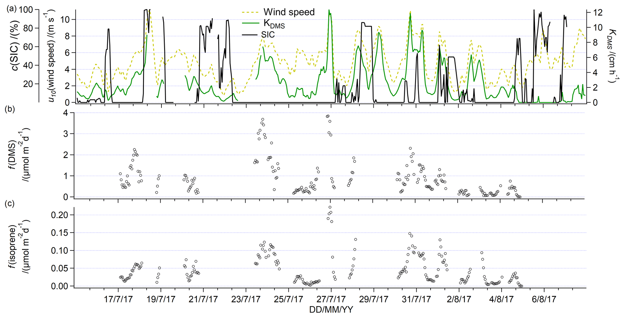
Figure 10(a) Underway sea ice concentration, wind speed at 10 m, and calculated air sea exchange velocity for DMS. Short gaps in the time series of the air sea exchange velocity of DMS are due to gaps in the recording of the underway sea surface temperature. Calculated underway fluxes of (b) DMS and (c) isoprene.
Atmospheric mixing ratios of these gases were not measured during this campaign. Therefore, we use a constant mixing ratio based on literature values to calculate fluxes and saturations, this is similar to methods used by Beale et al. (2015) for methanol and acetone. For methanol and acetone, we assume a constant mixing ratio of 0.3 and 0.4 ppbv, respectively, as measured by Sjostedt et al. (2012). Due to the lack of ambient air measurements during this cruise, the estimated fluxes of methanol and acetone are rather uncertain (i.e. the air–sea concentration difference is highly sensitive to atmospheric concentration, Yang et al., 2014a). Ambient air concentrations of isoprene and DMS generally have a small influence on the calculated air–sea flux due to the low solubility and large supersaturation (Baker et al., 2000; Matsunaga et al., 2002; Wohl et al., 2020) and the short lifetime of the compounds in the atmosphere (Chen et al., 2018; Medeiros et al., 2018). Thus, we assume the ambient air concentrations of isoprene to be zero in our flux estimates. For DMS, we assume a constant value of 0.1855 ppbv, as measured previously in this area at a similar time of year by Mungall et al. (2016). Assuming an ambient air concentration of zero for DMS could potentially lead to overestimations of the DMS flux (Zhang et al., 2020). Acetaldehyde fluxes were not computed due to the uncertainty in absolute acetaldehyde concentrations related to uncertain background corrections (Sect. S2). We use our underway measurements from 3–4 m depth to calculate air–sea fluxes, thus we do not account for the sometimes slightly higher seawater concentrations of some compounds observed at some stations at 30 cm depth, which could affect our flux estimates (as shown for CO2 in Dong et al., 2021).
We calculate a mean flux of methanol into the ocean of −3.3 µmol m−2 d−1 and a mean saturation of 22 %. The equilibrium gas-phase mixing ratio was 0.06 ppbv, suggesting that the flux of methanol was most likely consistently into the ocean. Direct flux measurements of methanol in the Labrador Sea and during a transatlantic crossing typically report −20 to −10 µmol m−2 d−1 but similar saturations of around 20 % (Yang et al., 2013a, 2014a). It is likely that the calculated methanol fluxes from this cruise are lower due to the low wind speeds during this cruise (Fig. 10) and sea ice acting as a barrier to air–sea exchange in this calculation. Oceanic uptake of methanol is probably due to the extremely high solubility of this compound combined with the relatively high air mixing ratios, characteristic of marine air in the Northern Hemisphere (Bates et al., 2021; Galbally et al., 2007).
The mean flux of acetone during this deployment is calculated to be into the ocean at −3.3 µmol m−2 d−1, while the mean saturation is 27 %. The equilibrium gas phase mixing ratio is calculated as 0.10 ppbv, which suggests that the acetone flux was largely into the ocean with episodes of outgassing possible. This mean flux is within the range of previous acetone flux measurements in the open ocean of typically around 10 to −10 µmol m−2 d−1 (Schlundt et al., 2017; Taddei et al., 2009; Yang et al., 2014a, b). Acetone was most likely undersaturated due to the relatively low seawater concentrations and high atmospheric mixing ratios that are characteristic of marine air in the Northern Hemisphere (Galbally et al., 2007; S. Wang et al., 2020).
In Fig. 10, we show wind speed, sea ice concentration, and estimated DMS transfer velocity, as well as the fluxes of DMS and isoprene. A cruise mean DMS flux of 0.89 µmol m−2 d−1 has been calculated, while the median is only 0.64 µmol m−2 d−1 (Fig. 10). This is within the range of directly measured DMS fluxes in the Labrador Sea in October and November of 1.5 µmol m−2 d−1 (Kim et al., 2017) or other calculated fluxes in the Canadian Arctic Archipelago of 0.2–12 µmol m−2 d−1 in July and August (Mungall et al., 2016). During the campaign presented here, the highest fluxes of DMS of around 3.8 µmol m−2 d−1 were observed on 24 and 27 July in ice-free conditions. These events of with the highest DMS emissions were marked by moderate wind speeds and near cruise average DMS seawater concentrations. They were both located in the Smith Sound area. On average, we observe higher mean DMS fluxes in Smith Sound (1.44 µmol m−2 d−1) compared to western Baffin Bay (1.12 µmol m−2 d−1) and Lancaster Sound (0.52 µmol m−2 d−1). Previous modelling studies found large marine contributions to atmospheric DMS mixing ratios in the Canadian Arctic from the Baffin Bay and Smith Sound area (Mungall et al., 2016).
The mean flux of isoprene during this deployment was 0.047 µmol m−2 d−1, while the median was 0.033 µmol m−2 d−1 (Fig. 10). These estimates are comparable to previous direct measurements of isoprene fluxes in the Labrador Sea of on average 0.0718 µmol m−2 d−1 (Kim et al., 2017) or other calculated fluxes in open ocean (Broadgate et al., 1997; Matsunaga et al., 2002). It is surprising that the relatively high isoprene concentrations measured throughout this cruise track did not lead to higher fluxes. Relatively low fluxes of isoprene despite high seawater concentrations are due to the low wind speeds from this cruise and sea ice acting as a barrier to air–sea exchange in our calculation. The mean isoprene flux is higher than the median, which suggests that isoprene fluxes are dominated by episodic emissions related to biological productivity, wind, and sea-ice-driven air–sea exchange. For example, as with DMS, the highest emissions of isoprene of up to 0.2 µmol m−2 d−1 were observed in the Smith Sound area on 24 July and 27 July. Indeed, isoprene fluxes were higher on average in Smith Sound (0.065 µmol m−2 d−1) compared to western Baffin Bay (0.041 µmol m−2 d−1) and Lancaster Sound as well (0.029 µmol m−2 d−1). These episodes in Smith Sound were marked by some of the highest wind speeds of the campaign (nearly 10 m s−1) and very low sea ice coverage. In fact, over this cruise track, isoprene and DMS fluxes correlate significantly. The correlation of the isoprene flux as a function of the DMS flux gives a slope of 0.038 and an intercept of 0.006 (R2=0.68; P<0.001; N=212). This suggests that DMS and isoprene tend to be emitted together in the same ice-free locations even if their underway seawater concentration did not significantly correlate. This is largely because fluxes in the sea ice zone tend to be controlled by wind speed and SIC, rather than seawater concentrations. In general, higher DMS and isoprene dissolved concentrations at higher SIC and highest emissions at low SIC and high winds suggests that both of these gases are produced at high SIC and released to the atmosphere when the ice retreats or when there are ice-free conditions.
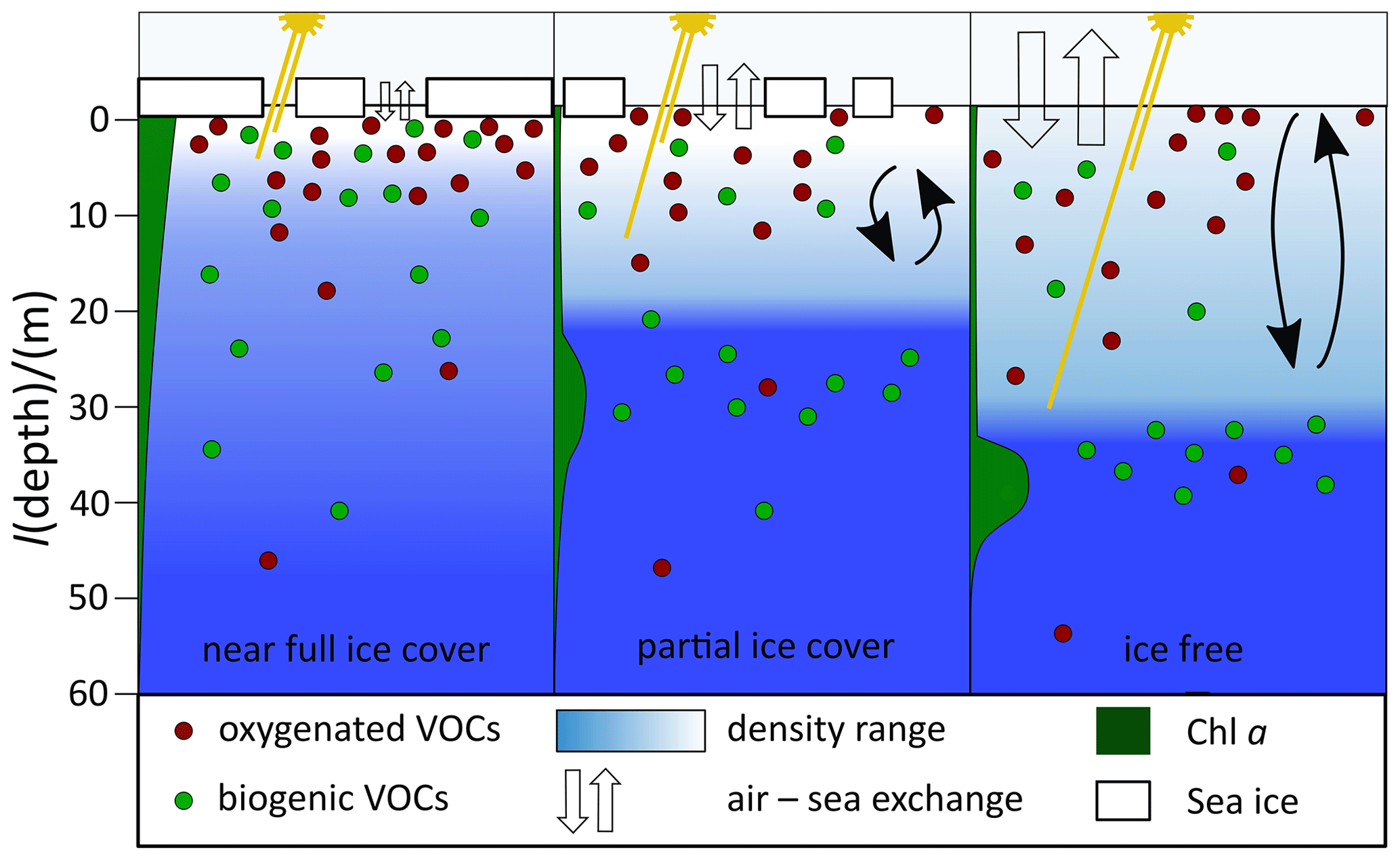
Figure 11Schematic summarizing the impact of seasonal sea ice melt on dissolved gas concentrations. Methanol, acetone and acetaldehyde are shown as “oxygenated VOCs”, and DMS and isoprene are shown as “biogenic VOCs”. The shorter light beam represents UV rays, while the longer one represents PAR.
To calculate the lifetime of isoprene in seawater relative to air–sea exchange, we assume an approximate mean mixed-layer depth of 15 m (estimated from Figs. 2 and 7), which is divided by the cruise mean isoprene transfer velocity (2.51 cm h−1). This gives a mean lifetime of isoprene with respect to air–sea exchange of 24 d. Previous authors have estimated this to be 7 (Palmer and Shaw, 2005) or 10 d (Booge et al., 2018). This implies that ventilation to the atmosphere is a smaller sink of isoprene during this cruise compared to the open ocean, possibly due to the low wind speeds characteristic of summer in this area (McLaughlin et al., 2004) and sea ice acting as a barrier to air–sea exchange. Reduced ventilation may also contribute to the relatively high isoprene seawater concentrations observed in the sea ice zone compared to open-ocean measurements.
This paper presents depth profiles and underway seawater measurements of methanol, acetone, acetaldehyde, DMS, and isoprene in the marginal sea ice zone. The measurements were taken in the Canadian Arctic Archipelago during July and August 2017, i.e. during Arctic summer and sea ice melt. To the best of our knowledge, these represent the first measurements of seawater concentrations of methanol, acetone, acetaldehyde, and isoprene in the Canadian Arctic Archipelago. The underway measurements are also used to calculate air–sea fluxes.
To synthesize the observations, a summary of the effect of different sea ice concentrations on dissolved gas distributions is provided here as a schematic (Fig. 11).
For ease of illustration and discussion, here we group methanol, acetone, and acetaldehyde as “oxygenated VOCs” and DMS and isoprene as “biogenic VOCs”.
Oxygenated VOCs tend to display the highest concentrations near the surface and do not display a subsurface maximum. They often display slightly higher concentrations at 30 cm compared to 2 or 5 m if a surface stratified layer is present. Underway methanol concentrations display a large range in concentration in the sea ice zone and generally higher concentrations near the surface in ice-free waters. This appears to be consistent with rapid biological cycling (Mincer and Aicher, 2016; Sargeant et al., 2016) where the sources and sinks are at times decoupled. Acetone and acetaldehyde concentrations decline rapidly from the surface to reach a constant value at about 5 m in near-full ice cover and at about 20 to 30 m in partial ice cover (less than 50 % SIC) and ice-free waters. This is probably due to deeper UV light penetration at lower SIC and increased mixing as the mixed layer forms after ice breakup. Higher concentrations in the top 5 m of the water column support a dominant photochemical, UV-light-dependent source of these compounds in the sea ice zone, as wavelengths required for biological production would be expected to penetrate deeper. Despite obvious sources in seawater, we calculate that the sea ice zone is highly undersaturated in methanol and acetone relative to the atmosphere, leading to net ocean uptake of these gases.
The biogenic VOCs, DMS and isoprene, behave differently to the oxygenated VOCs in that they sometimes display a subsurface maximum. DMS concentrations are higher at 30 cm than at 5 m in high ice cover, possibly due to ice-related algae. Isoprene more often displays higher concentrations at 30 cm, an effect that seems independent of the sea ice concentration at the time of sampling. In casts with high ice cover (75 % to 90 % SIC), we observe gradual declines of DMS and isoprene concentrations from the surface down to about 50 m. In partial ice cover and in ice-free conditions (less than 50 % SIC), DMS and isoprene concentrations in the mixed layer are more homogenous. Many of these casts display a deep isoprene maximum but only sometimes a deep DMS maximum. Isoprene and DMS surface concentrations were both higher at higher SIC. Our measured DMS concentrations were lower than previous observations in this area and around this time of year as we most likely sampled after the annual peak phytoplankton bloom. Surface isoprene concentrations correlated more strongly with SIC than with SST or Chl a, suggesting that isoprene concentrations in the sea ice zone are controlled by different processes than in the open ocean. DMS and isoprene fluxes were tightly correlated, even if their seawater concentrations were not. Higher emissions of biogenic VOCs were observed in ice-free areas than those with heavy sea ice cover. Our calculation of the lifetime of isoprene relative to air–sea exchange suggests that sea ice leads to reduced ventilation of isoprene and thus a longer lifetime of dissolved isoprene in the sea ice zone compared to open ocean. This contributes to relatively high seawater isoprene concentrations in the sea ice zone.
Taken together, our observations suggest that sea ice concentration exerts a strong influence on dissolved VOCs via an interplay between physical drivers (e.g. mixing, seasonal stratification, light penetration, wind speed) and biogeochemistry. These measurements and insights improve our understanding of the cycling of these gases in the polar oceans. The air–sea fluxes of DMS and isoprene will be helpful for improving estimates of the aerosol budgets in the changing Arctic. Simultaneous emission of DMS and isoprene suggests that they are part of the cocktail of gases released into the atmosphere from the recent ice-uncovered water column. Similarly, the air–sea fluxes of methanol and acetone will be helpful to assess the impact of these oxygenated VOCs on the oxidative capacity of the atmosphere.
With further sea ice loss predicted for a changing Arctic, we speculate that this is going to lead to higher emissions of biogenic VOCs in the future. For example, sea ice loss over the last approximately 20 years has led to increased emissions of DMS (Galí et al., 2019), which also affected aerosol concentrations in summer (Sharma et al., 2012). Due to increased sea ice loss and the subsequent increase in air-to-sea flux, we speculate that the Arctic Ocean will be a bigger sink for oxygenated VOCs, thereby probably reducing their atmospheric concentration.
Further campaigns should focus on year-round observations at the same site to reduce some of the variability in our dataset due to heterogenous sea ice biogeochemistry and local oceanography. Additionally, Lagrangian experiments would be useful to better understand the effect of water masses moving along sea ice edges. Future analysis should focus on how long the water column has been ice uncovered, which has been shown to influence dissolved CO2 (Ahmed et al., 2019) and DMS (Galí et al., 2021).
Data have been submitted to Polar Data Catalogue (https://www.polardata.ca/pdcsearch/), where the CCIN Reference number is 13249 and the DOI is https://doi.org/10.21963/13249.
The supplement related to this article is available online at: https://doi.org/10.5194/bg-19-1021-2022-supplement.
MY, AEJ, WTS, and PDN conceptualized the project. CW carried out the measurements and data analysis. BE provided crucial resources for the project. BJB provided the wind speed measurements. CW wrote the manuscript with input from all co-authors.
The contact author has declared that neither they nor their co-authors have any competing interests.
Publisher's note: Copernicus Publications remains neutral with regard to jurisdictional claims in published maps and institutional affiliations.
These measurements were made possible through a large range of collaborations. We are thankful to Mohamed Ahmed, Dave Capelle, Tonya Burgers, Douglas Collins, Jonathan Abbatt, and Martine Lizotte for logistical support. We thank Jean-Éric Tremblay for contributing the nitrate measurements. Many thanks to Emily Alcock for her support during the write up. Final thanks go to the excellent crew of the CCGS Amundsen and the chief scientists Jean-Éric Tremblay and Martine Lizotte. Some of the data presented herein were collected by the Canadian research icebreaker CCGS Amundsen and made available by the Amundsen Science program, which is supported by the Canada Foundation for Innovation Major Science Initiatives Fund. The views expressed in this publication do not necessarily represent the views of Amundsen Science or those of its partners. We thank the Institute of Environmental Physics at the University of Bremen for the provision of the merged MODIS-AMSR2 sea ice concentration data at https://seaice.uni-bremen.de/data/modis_amsr2/ (last access: 11 January 2019).
This work was supported by the Natural Environment Research Council through the EnvEast Doctoral Training Partnership (grant no. NE/L002582/1) and by the UK Department for Business, Energy and Industrial Strategy (United Kingdom & Canada Arctic Partnership: 2017 Bursaries Programme awarded to MY). Financial support was provided to Brent Else by the National Sciences and Engineering Research Council of Canada. This work is a contribution to ArcticNet, a Network of Centres of Excellence Canada.
This paper was edited by Gwenaël Abril and reviewed by Miming Zhang and two anonymous referees.
Abbatt, J. P. D., Leaitch, W. R., Aliabadi, A. A., Bertram, A. K., Blanchet, J.-P., Boivin-Rioux, A., Bozem, H., Burkart, J., Chang, R. Y. W., Charette, J., Chaubey, J. P., Christensen, R. J., Cirisan, A., Collins, D. B., Croft, B., Dionne, J., Evans, G. J., Fletcher, C. G., Galí, M., Ghahremaninezhad, R., Girard, E., Gong, W., Gosselin, M., Gourdal, M., Hanna, S. J., Hayashida, H., Herber, A. B., Hesaraki, S., Hoor, P., Huang, L., Hussherr, R., Irish, V. E., Keita, S. A., Kodros, J. K., Köllner, F., Kolonjari, F., Kunkel, D., Ladino, L. A., Law, K., Levasseur, M., Libois, Q., Liggio, J., Lizotte, M., Macdonald, K. M., Mahmood, R., Martin, R. V., Mason, R. H., Miller, L. A., Moravek, A., Mortenson, E., Mungall, E. L., Murphy, J. G., Namazi, M., Norman, A.-L., O'Neill, N. T., Pierce, J. R., Russell, L. M., Schneider, J., Schulz, H., Sharma, S., Si, M., Staebler, R. M., Steiner, N. S., Thomas, J. L., von Salzen, K., Wentzell, J. J. B., Willis, M. D., Wentworth, G. R., Xu, J.-W., and Yakobi-Hancock, J. D.: Overview paper: New insights into aerosol and climate in the Arctic, Atmos. Chem. Phys., 19, 2527–2560, https://doi.org/10.5194/acp-19-2527-2019, 2019.
Ahmed, M., Else, B. G. T., Burgers, T. M., and Papakyriakou, T.: Variability of Surface Water pCO2 in the Canadian Arctic Archipelago From 2010 to 2016, J. Geophys. Res.-Oceans, 124, 1876–1896, https://doi.org/10.1029/2018JC014639, 2019.
Ahmed, M. M. M., Else, B. G. T., Capelle, D., Miller, L. A., and Papakyriakou, T.: Underestimation of surface pCO2 and air-sea CO2 fluxes due to freshwater stratification in an Arctic shelf sea, Hudson Bay, Elem. Sci. Anthr., 9, 1–21, 2020.
Amundsen Science Data Collection: TSG and CTD data collected by the CCGS Amundsen in the Canadian Arctic. Processed data, TSG Version 2, CTD Version 1, available at: https://polardata.ca/, Canadian Cryospheric Information Network (CCIN), ArcticNet Inc., Québec, Canada, https://doi.org/10.5884/12715, 2017.
Ardyna, M., Babin, M., Gosselin, M., Devred, E., Bélanger, S., Matsuoka, A., and Tremblay, J.-É.: Parameterization of vertical Chlorophyll a in the Arctic Ocean: impact of the subsurface chlorophyll maximum on regional, seasonal, and annual primary production estimates, Biogeosciences, 10, 4383–4404, https://doi.org/10.5194/bg-10-4383-2013, 2013.
Arnold, S. R., Spracklen, D. V., Williams, J., Yassaa, N., Sciare, J., Bonsang, B., Gros, V., Peeken, I., Lewis, A. C., Alvain, S., and Moulin, C.: Evaluation of the global oceanic isoprene source and its impacts on marine organic carbon aerosol, Atmos. Chem. Phys., 9, 1253–1262, https://doi.org/10.5194/acp-9-1253-2009, 2009.
Arrigo, K. R., Matrai, P. A., and Van Dijken, G. L.: Primary productivity in the Arctic Ocean: Impacts of complex optical properties and subsurface chlorophyll maxima on large-scale estimates, J. Geophys. Res.-Oceans, 116, 1–15, https://doi.org/10.1029/2011JC007273, 2011.
Baker, A. R., Turner, S. M., Broadgate, W. J., Thompson, A., McFiggans, G. B., Vesperini, O., Nightingal, P. D., Liss, P. S., and Jickells, T. D.: Distribution and sea-air fluxes of biogenic trace gases in the eastern Atlantic Ocean, Global Biogeochem. Cy., 14, 871–886, https://doi.org/10.1029/1999GB001219, 2000.
Barber, D. G., Hop, H., Mundy, C. J., Else, B., Dmitrenko, I. A., Tremblay, J. E., Ehn, J. K., Assmy, P., Daase, M., Candlish, L. M., and Rysgaard, S.: Selected physical, biological and biogeochemical implications of a rapidly changing Arctic Marginal Ice Zone, Prog. Oceanogr., 139, 122–150, https://doi.org/10.1016/j.pocean.2015.09.003, 2015.
Bates, K. H., Jacob, D. J., Wang, S., Hornbrook, R. S., Apel, E. C., Kim, M. J., Millet, D. B., Wells, K. C., Chen, X., Brewer, J. F., Ray, E. A., Commane, R., Diskin, G. S., and Wofsy, S. C.: The global budget of atmospheric methanol: new constraints on secondary, oceanic, and terrestrial sources, J. Geophys. Res.-Atmos., 126, 1–23, https://doi.org/10.1029/2020jd033439, 2021.
Beale, R., Dixon, J. L., Arnold, S. R., Liss, P. S., and Nightingale, P. D.: Methanol, acetaldehyde, and acetone in the surface waters of the Atlantic Ocean, J. Geophys. Res.-Oceans, 118, 5412–5425, https://doi.org/10.1002/jgrc.20322, 2013.
Beale, R., Dixon, J. L., Smyth, T. J., and Nightingale, P. D.: Annual study of oxygenated volatile organic compounds in UK shelf waters, Mar. Chem., 171, 96–106, https://doi.org/10.1016/j.marchem.2015.02.013, 2015.
Beaupré-Laperrière, A., Mucci, A., and Thomas, H.: The recent state and variability of the carbonate system of the Canadian Arctic Archipelago and adjacent basins in the context of ocean acidification, Biogeosciences, 17, 3923–3942, https://doi.org/10.5194/bg-17-3923-2020, 2020.
Booge, D., Schlundt, C., Bracher, A., Endres, S., Zäncker, B., and Marandino, C. A.: Marine isoprene production and consumption in the mixed layer of the surface ocean – a field study over two oceanic regions, Biogeosciences, 15, 649–667, https://doi.org/10.5194/bg-15-649-2018, 2018.
Bouillon, R. C., Lee, P. A., De Mora, S. J., Levasseur, M., and Lovejoy, C.: Vernal distribution of dimethylsulphide, dimethylsulphoniopropionate, and dimethylsulphoxide in the North Water in 1998, Deep. Res. Pt II, 49, 5171–5189, https://doi.org/10.1016/S0967-0645(02)00184-4, 2002.
Broadgate, W. J., Liss, P. S., Penkett, S. A., and Penkett, A.: Seasonal emissions of isoprene and other reactive hydrocarbon gases from the ocean, Geophys. Res. Lett., 24, 2675–2678, https://doi.org/10.1029/97GL02736, 1997.
de Bruyn, W. J., Clark, C. D., Pagel, L., and Singh, H.: Loss rates of acetone in filtered and unfiltered coastal seawater, Mar. Chem., 150, 39–44, https://doi.org/10.1016/j.marchem.2013.01.003, 2013.
de Bruyn, W. J., Clark, C. D., Senstad, M., Barashy, O., and Hok, S.: The biological degradation of acetaldehyde in coastal seawater, Mar. Chem., 192, 13–21, https://doi.org/10.1016/j.marchem.2017.02.008, 2017.
de Bruyn, W. J., Clark, C. D., Harrison, A. W., Senstad, M., and Hok, S.: The degradation of acetaldehyde in estuary waters in Southern California, USA, Environ. Sci. Pollut. Res., 28, 35811–35821, https://doi.org/10.1007/s11356-021-13232-x, 2021.
de Bruyn, W. J., Clark, C. D., Pagel, L., and Takehara, C.: Photochemical production of formaldehyde, acetaldehyde and acetone from chromophoric dissolved organic matter in coastal waters, J. Photochem. Photobiol. A Chem., 226, 16–22, https://doi.org/10.1016/j.jphotochem.2011.10.002, 2011.
Burgers, T. M., Tremblay, J.-É., Else, B. G. T., and Papakyriakou, T. N.: Estimates of net community production from multiple approaches surrounding the spring ice-edge bloom in Baffin Bay, Elem. Sci. Anthr., 8, https://doi.org/10.1525/elementa.013, 2020.
Burt, W. J., Thomas, H., Miller, L. A., Granskog, M. A., Papakyriakou, T. N., and Pengelly, L.: Inorganic carbon cycling and biogeochemical processes in an Arctic inland sea (Hudson Bay), Biogeosciences, 13, 4659–4671, https://doi.org/10.5194/bg-13-4659-2016, 2016.
Butterworth, B. J. and Miller, S. D.: Air-sea exchange of carbon dioxide in the Southern Ocean and Antarctic marginal ice zone, Geophys. Res. Lett., 43, 7223–7230, https://doi.org/10.1002/2016GL069581, 2016.
Chen, Q., Sherwen, T., Evans, M., and Alexander, B.: DMS oxidation and sulfur aerosol formation in the marine troposphere: a focus on reactive halogen and multiphase chemistry, Atmos. Chem. Phys., 18, 13617–13637, https://doi.org/10.5194/acp-18-13617-2018, 2018.
Collins, D. B., Burkart, J., Chang, R. Y.-W., Lizotte, M., Boivin-Rioux, A., Blais, M., Mungall, E. L., Boyer, M., Irish, V. E., Massé, G., Kunkel, D., Tremblay, J.-É., Papakyriakou, T., Bertram, A. K., Bozem, H., Gosselin, M., Levasseur, M., and Abbatt, J. P. D.: Frequent ultrafine particle formation and growth in Canadian Arctic marine and coastal environments, Atmos. Chem. Phys., 17, 13119–13138, https://doi.org/10.5194/acp-17-13119-2017, 2017.
Dai, A., Luo, D., Song, M., and Liu, J.: Arctic amplification is caused by sea-ice loss under increasing CO2, Nat. Commun., 10, 1–13, https://doi.org/10.1038/s41467-018-07954-9, 2019.
Dall'Osto, M., Beddows, D. C. S., Tunved, P., Krejci, R., Ström, J., Hansson, H. C., Yoon, Y. J., Park, K. T., Becagli, S., Udisti, R., Onasch, T., Ódowd, C. D., Simó, R., and Harrison, R. M.: Arctic sea ice melt leads to atmospheric new particle formation, Sci. Rep., 7, 1–10, https://doi.org/10.1038/s41598-017-03328-1, 2017.
Dall'Osto, M., Geels, C., Beddows, D. C. S., Boertmann, D., Lange, R., Nøjgaard, J. K., Harrison, R. M., Simo, R., Skov, H., and Massling, A.: Regions of open water and melting sea ice drive new particle formation in North East Greenland, Sci. Rep., 8, 1–10, https://doi.org/10.1038/s41598-018-24426-8, 2018.
Dani, K. G. S. and Loreto, F.: Trade-Off Between Dimethyl Sulfide and Isoprene Emissions from Marine Phytoplankton, Trends Plant Sci., 22, 1–12, https://doi.org/10.1016/j.tplants.2017.01.006, 2017.
Davie-Martin, C. L., Giovannoni, S. J., Behrenfeld, M. J., Penta, W. B., and Halsey, K. H.: Seasonal and spatial variability in the biogenic production and consumption of volatile organic compounds (VOCs) by marine plankton in the North Atlantic Ocean, Front. Mar. Sci., 7, 1–15, https://doi.org/10.3389/fmars.2020.611870, 2020.
Dixon, J. L. and Nightingale, P. D.: Fine-scale variability in methanol uptake and oxidation: from the microlayer to 1000 m, Biogeosciences, 9, 2961–2972, https://doi.org/10.5194/bg-9-2961-2012, 2012.
Dixon, J. L., Beale, R., and Nightingale, P. D.: Rapid biological oxidation of methanol in the tropical Atlantic: significance as a microbial carbon source, Biogeosciences, 8, 2707–2716, https://doi.org/10.5194/bg-8-2707-2011, 2011.
Dixon, J. L., Beale, R., and Nightingale, P. D.: Production of methanol, acetaldehyde, and acetone in the Atlantic Ocean, Geophys. Res. Lett., 40, 4700–4705, https://doi.org/10.1002/grl.50922, 2013.
Dixon, J. L., Beale, R., Sargeant, S. L., Tarran, G. A., and Nightingale, P. D.: Microbial acetone oxidation in coastal seawater, Front. Microb., 5, 1–9, https://doi.org/10.3389/fmicb.2014.00243, 2014.
Dong, Y., Yang, M., Bakker, D. C. E., Liss, P. S., Kitidis, V., Brown, I., Chierici, M., Fransson, A., and Bell, T. G.: Near-Surface Stratification Due to Ice Melt Biases Arctic Air-Sea CO2 Flux Estimates, Geophys. Res. Lett., 48, 1–10, https://doi.org/10.1029/2021GL095266, 2021.
Galbally, I. E., Lawson, S. J., Weeks, I. A., Bentley, S. T., Gillett, R. W., Meyer, M., and Goldstein, A. H.: Volatile organic compounds in marine air at Cape Grim, Australia, Environ. Chem., 4, 178–182, https://doi.org/10.1071/EN07024, 2007.
Galí, M. and Simó, R.: Occurrence and cycling of dimethylated sulfur compounds in the Arctic during summer receding of the ice edge, Mar. Chem., 122, 105–117, https://doi.org/10.1016/j.marchem.2010.07.003, 2010.
Galí, M., Levasseur, M., Devred, E., Simó, R., and Babin, M.: Sea-surface dimethylsulfide (DMS) concentration from satellite data at global and regional scales, Biogeosciences, 15, 3497–3519, https://doi.org/10.5194/bg-15-3497-2018, 2018.
Galí, M., Devred, E., Babin, M., and Levasseur, M.: Decadal increase in Arctic dimethylsulfide emission, P. Natl. Acad. Sci. USA, 116, 19311–19317, https://doi.org/10.1073/pnas.1904378116, 2019.
Galí, M., Lizotte, M., Kieber, D. J., Randelhoff, A., Hussherr, R., Xue, L., Dinasquet, J., Babin, M., Rehm, E., and Levasseur, M.: DMS emissions from the Arctic marginal ice zone, Elem. Sci. Anthr., 9, 1–31, https://doi.org/10.1525/elementa.2020.00113, 2021.
Gourdal, M., Lizotte, M., Massé, G., Gosselin, M., Poulin, M., Scarratt, M., Charette, J., and Levasseur, M.: Dimethyl sulfide dynamics in first-year sea ice melt ponds in the Canadian Arctic Archipelago, Biogeosciences, 15, 3169–3188, https://doi.org/10.5194/bg-15-3169-2018, 2018.
Granskog, M. A., Pavlov, A. K., Sagan, S., Kowalczuk, P., Raczkowska, A., and Stedmon, C. A.: Effect of sea-ice melt on inherent optical properties and vertical distribution of solar radiant heating in Arctic surface waters, J. Geophys. Res.-Oceans, 120, 775–791, https://doi.org/10.1002/2015JC011107, 2015.
Hackenberg, S. C., Andrews, S. J., Airs, R., Arnold, S. R., Bouman, H. A., Brewin, R. J. W., Chance, R. J., Cummings, D., Dall'Olmo, G., Lewis, A. C., Minaeian, J. K., Reifel, K. M., Small, A., Tarran, G. A., Tilstone, G. H., and Carpenter, L. J.: Potential controls of isoprene in the surface ocean, Global Biogeochem. Cy., 31, 644–662, https://doi.org/10.1002/2016GB005531, 2017.
Halsey, K. H., Giovannoni, S. J., Graus, M., Zhao, Y., Landry, Z., Thrash, J. C., Vergin, K. L., and de Gouw, J. A.: Biological cycling of volatile organic carbon by phytoplankton and bacterioplankton, Limnol. Oceanogr., 62, 2650–2661, https://doi.org/10.1002/lno.10596, 2017.
Hayashida, H., Carnat, G., Galí, M., Monahan, A. H., Mortenson, E., Sou, T., and Steiner, N. S.: Spatiotemporal Variability in Modeled Bottom Ice and Sea Surface Dimethylsulfide Concentrations and Fluxes in the Arctic During 1979–2015, Global Biogeochem. Cy., 34, e2019GB006456, https://doi.org/10.1029/2019GB006456, 2020.
Hudson, E. D., Okuda, K., and Ariya, P. A.: Determination of acetone in seawater using derivatization solid-phase microextraction, Anal. Bioanal. Chem., 388, 1275–1282, https://doi.org/10.1007/s00216-007-1324-x, 2007.
Hulswar, S., Simo, R., Galí, M., Bell, T., Lana, A., Inamdar, S., Halloran, P. R., Manville, G., and Mahajan, A. S.: Third Revision of the Global Surface Seawater Dimethyl Sulfide Climatology (DMS-Rev3), Earth Syst. Sci. Data Discuss. [preprint], https://doi.org/10.5194/essd-2021-236, in review, 2021.
Huntington, H. P., Carey, M., Apok, C., Forbes, B. C., Fox, S., Holm, L. K., Ivanova, A., Jaypoody, J., Noongwook, G., and Stammler, F.: Climate change in context: putting people first in the Arctic, Reg. Environ. Chang., 19, 1217–1223, https://doi.org/10.1007/s10113-019-01478-8, 2019.
Jarníková, T., Dacey, J., Lizotte, M., Levasseur, M., and Tortell, P.: The distribution of methylated sulfur compounds, DMS and DMSP, in Canadian subarctic and Arctic marine waters during summer 2015, Biogeosciences, 15, 2449–2465, https://doi.org/10.5194/bg-15-2449-2018, 2018.
Johnson, M. T.: A numerical scheme to calculate temperature and salinity dependent air-water transfer velocities for any gas, Ocean Sci., 6, 913–932, https://doi.org/10.5194/os-6-913-2010, 2010.
Kaimal, J. C. and Finnigan, J. J.: Atmospheric boundary layer flows – their structure and measurement, Oxford University Press., https://doi.org/10.1093/oso/9780195062397.001.0001, 1994.
Kameyama, S., Tanimoto, H., Inomata, S., Tsunogai, U., Ooki, A., Takeda, S., Obata, H., Tsuda, A., and Uematsu, M.: High-resolution measurement of multiple volatile organic compounds dissolved in seawater using equilibrator inlet-proton transfer reaction-mass spectrometry (EI-PTR-MS), Mar. Chem., 122, 59–73, https://doi.org/10.1016/j.marchem.2010.08.003, 2010.
Kameyama, S., Tanimoto, H., Inomata, S., Suzuki, K., Komatsu, D. D., Hirota, A., Konno, U., and Tsunogai, U.: Application of PTR-MS to an incubation experiment of the marine diatom Thalassiosira pseudonana, Geochem. J., 45, 355–363, https://doi.org/10.2343/geochemj.1.0127, 2011.
Kieber, R., Zhou, X., and Mopper, K.: Formation of carbonyl-compounds from UV-induced photodegradation of humic substances in natural-waters – fate of riverine carbon in the sea, Limnol. Oceanogr., 35, 1503–1515, 1990.
Kiene, R. P. and Bates, T. S.: Biological removal of dimethyl sulphide from sea water, Nature, 345, 702–705, https://doi.org/10.1038/258748a0, 1990.
Kim, M. J., Novak, G. A., Zoerb, M. C., Yang, M., Blomquist, B. W., Huebert, B. J., Cappa, C. D., and Bertram, T. H.: Air-Sea exchange of biogenic volatile organic compounds and the impact on aerosol particle size distributions, Geophys. Res. Lett., 44, 3887–3896, https://doi.org/10.1002/2017GL072975, 2017.
Köllner, F., Schneider, J., Willis, M. D., Klimach, T., Helleis, F., Bozem, H., Kunkel, D., Hoor, P., Burkart, J., Leaitch, W. R., Aliabadi, A. A., Abbatt, J. P. D., Herber, A. B., and Borrmann, S.: Particulate trimethylamine in the summertime Canadian high Arctic lower troposphere, Atmos. Chem. Phys., 17, 13747–13766, https://doi.org/10.5194/acp-17-13747-2017, 2017.
Lana, A., Bell, T. G., Simó, R., Vallina, S. M., Ballabrera-Poy, J., Kettle, A. J., Dachs, J., Bopp, L., Saltzman, E. S., Stefels, J., Johnson, J. E., and Liss, P. S.: An updated climatology of surface dimethlysulfide concentrations and emission fluxes in the global ocean, Global Biogeochem. Cy., 25, GB1004, https://doi.org/10.1029/2010GB003850, 2011.
Levasseur, M.: Impact of Arctic meltdown on the microbial cycling of sulphur, Nat. Geosci., 6, 691–700, https://doi.org/10.1038/ngeo1910, 2013.
Liss, P. S. and Slater, P. G.: Flux of Gases across the Air-Sea Interface, Nature, 247, 181–184, https://doi.org/10.1038/247181a0, 1974.
Lizotte, M., Levasseur, M., Galindo, V., Gourdal, M., Gosselin, M., Tremblay, J.-É., Blais, M., Charette, J., and Hussherr, R.: Phytoplankton and dimethylsulfide dynamics at two contrasting Arctic ice edges, Biogeosciences, 17, 1557–1581, https://doi.org/10.5194/bg-17-1557-2020, 2020.
Loose, B., McGillis, W. R., Perovich, D., Zappa, C. J., and Schlosser, P.: A parameter model of gas exchange for the seasonal sea ice zone, Ocean Sci., 10, 17–28, https://doi.org/10.5194/os-10-17-2014, 2014.
Luce, M., Levasseur, M., Scarratt, M. G., Michaud, S., Royer, S. J., Kiene, R., Lovejoy, C., Gosselin, M., Poulin, M., Gratton, Y., and Lizotte, M.: Distribution and microbial metabolism of dimethylsulfoniopropionate and dimethylsulfide during the 2007 Arctic ice minimum, J. Geophys. Res.-Oceans, 116, 4–11, https://doi.org/10.1029/2010JC006914, 2011.
Mahmood, R., von Salzen, K., Norman, A.-L., Galí, M., and Levasseur, M.: Sensitivity of Arctic sulfate aerosol and clouds to changes in future surface seawater dimethylsulfide concentrations, Atmos. Chem. Phys., 19, 6419–6435, https://doi.org/10.5194/acp-19-6419-2019, 2019.
Marandino, C. A., de Bruyn, W. J., Miller, S. D., Prather, M. J., and Saltzman, E. S.: Oceanic uptake and the global atmospheric acetone budget, Geophys. Res. Lett., 32, 1–4, https://doi.org/10.1029/2005GL023285, 2005.
Markus, T., Stroeve, J. C., and Miller, J.: Recent changes in Arctic sea ice melt onset, freezeup, and melt season length, J. Geophys. Res.-Oceans, 114, 1–14, https://doi.org/10.1029/2009JC005436, 2009.
Martin, J., Tremblay, J. É., Gagnon, J., Tremblay, G., Lapoussière, A., Jose, C., Poulin, M., Gosselin, M., Gratton, Y., and Michel, C.: Prevalence, structure and properties of subsurface chlorophyll maxima in Canadian Arctic waters, Mar. Ecol. Prog. Ser., 412, 69–84, https://doi.org/10.3354/meps08666, 2010.
Massicotte, P., Bécu, G., Lambert-Girard, S., Leymarie, E., and Babin, M.: Estimating underwater light regime under spatially heterogeneous sea ice in the Arctic, Appl. Sci., 8, 1–19, https://doi.org/10.3390/app8122693, 2018.
Matsunaga, S., Mochida, M., Saito, T., and Kawamura, K.: In situ measurement of isoprene in the marine air and surface seawater from the western North Pacific, Atmos. Environ., 36, 6051–6057, https://doi.org/10.1016/S1352-2310(02)00657-X, 2002.
McLaughlin, F. A., Carmack, E. C., Ingram, R. G., Williams, W. J., and Michel, C.: Chapter 31: Oceanography of the Northwest Passage, The Sea, 14, 1211–1242, 2004.
Medeiros, D. J., Blitz, M. A., James, L., Speak, T. H., and Seakins, P. W.: Kinetics of the Reaction of OH with Isoprene over a Wide Range of Temperature and Pressure Including Direct Observation of Equilibrium with the OH Adducts, J. Phys. Chem. A, 122, 7239–7255, https://doi.org/10.1021/acs.jpca.8b04829, 2018.
Meier, W. N., Hovelsrud, G. K., VanOort, B. E. H., Key, J. R., Kovacs, K., Michel, C., Haas, C., Granskog, M. A., Gerland, S., Perovich, D. K., Makshtas, A., and Reist, J. D.: Arctic sea ice in transformation: A review of recent observed changes and impacts on biology and human activity, Rev. Geophys., 51, 185–217, https://doi.org/10.1002/ 2013RG000431, 2014.
Melling, H., Gratton, Y., and Ingram, G.: Ocean circulation within the North Water polynya of Baffin Bay, Atmos. Ocean, 39, 301–325, https://doi.org/10.1080/07055900.2001.9649683, 2001.
Miller, L. A., Burgers, T. M., Burt, W. J., Granskog, M. A., and Papakyriakou, T. N.: Air-Sea CO2 Flux Estimates in Stratified Arctic Coastal Waters: How Wrong Can We Be?, Geophys. Res. Lett., 46, 235–243, https://doi.org/10.1029/2018GL080099, 2019.
Mincer, T. J. and Aicher, A. C.: Methanol production by a broad phylogenetic array of marine phytoplankton, PLoS One, 11, 1–17, https://doi.org/10.1371/journal.pone.0150820, 2016.
Mopper, K. and Stahovec, W. L.: Sources and sinks of low molecular weight organic carbonyl compounds in seawater, Mar. Chem., 19, 305–321, https://doi.org/10.1016/0304-4203(86)90052-6, 1986.
Motard-Côté, J., Levasseur, M., Scarratt, M. G., Michaud, S., Gratton, Y., Rivkin, R. B., Keats, K., Gosselin, M., Tremblay, J. É., Kiene, R. P., and Lovejoy, C.: Distribution and metabolism of dimethylsulfoniopropionate (DMSP) and phylogenetic affiliation of DMSP-assimilating bacteria in northern Baffin Bay/Lancaster Sound, J. Geophys. Res.-Oceans, 117, C00G11, https://doi.org/10.1029/2011JC007330, 2012.
Münchow, A., Falkner, K. K., and Melling, H.: Baffin Island and West Greenland Current Systems in northern Baffin Bay, Prog. Oceanogr., 132, 305–317, https://doi.org/10.1016/j.pocean.2014.04.001, 2015.
Mungall, E. L., Croft, B., Lizotte, M., Thomas, J. L., Murphy, J. G., Levasseur, M., Martin, R. V., Wentzell, J. J. B., Liggio, J., and Abbatt, J. P. D.: Dimethyl sulfide in the summertime Arctic atmosphere: measurements and source sensitivity simulations, Atmos. Chem. Phys., 16, 6665–6680, https://doi.org/10.5194/acp-16-6665-2016, 2016.
Mungall, E. L., Abbatt, J. P. D., Wentzell, J. J. B., Lee, A. K. Y., Thomas, J. L., Blais, M., Gosselin, M., Miller, L. A., Papakyriakou, T., Willis, M. D., and Liggio, J.: A novel source of oxygenated volatile organic compounds in the summertime marine Arctic boundary layer, P. Natl. Acad. Sci. USA, 114, 6203–6208, https://doi.org/10.1073/pnas.1620571114, 2017.
Mungall, E. L., Abbatt, J. P. D., Wentzell, J. J. B., Wentworth, G. R., Murphy, J. G., Kunkel, D., Gute, E., Tarasick, D. W., Sharma, S., Cox, C. J., Uttal, T., and Liggio, J.: High gas-phase mixing ratios of formic and acetic acid in the High Arctic, Atmos. Chem. Phys., 18, 10237–10254, https://doi.org/10.5194/acp-18-10237-2018, 2018.
Nightingale, P. D., Malin, G., Law, C. S., Watson, J., Liss, P. S., and Liddicoat, I.: In situ evaluation of air-sea gas exchange parameterizations using novel conservative and volatile tracers, Global Biogeochem. Cy., 14, 373–387, https://doi.org/10.1029/1999GB900091, 2000.
Ooki, A., Nomura, D., Nishino, S., Kikuchi, T., and Yokouchi, Y.: A global-scale map of isoprene and volatile organic iodine in surface seawater of the Arctic, Northwest Pacific, Indian, and Southern Oceans, J. Geophys. Res.-Oceans, 120, 4108–4128, https://doi.org/10.1002/2014JC010519, 2015.
Ooki, A., Shida, R., Otsu, M., Onishi, H., Kobayashi, N., Iida, T., Nomura, D., Suzuki, K., Yamaoka, H., and Takatsu, T.: Isoprene production in seawater of Funka Bay, Hokkaido, Japan, J. Oceanogr., 75, 485–501, https://doi.org/10.1007/s10872-019-00517-6, 2019.
Paasonen, P., Asmi, A., Petäjä, T., Kajos, M. K., Äijälä, M., Junninen, H., Holst, T., Abbatt, J. P. D., Arneth, A., Birmili, W., Van Der Gon, H. D., Hamed, A., Hoffer, A., Laakso, L., Laaksonen, A., Richard Leaitch, W., Plass-Dülmer, C., Pryor, S. C., Räisänen, P., Swietlicki, E., Wiedensohler, A., Worsnop, D. R., Kerminen, V. M., and Kulmala, M.: Warming-induced increase in aerosol number concentration likely to moderate climate change, Nat. Geosci., 6, 438–442, https://doi.org/10.1038/ngeo1800, 2013.
Palmer, P. I. and Shaw, S. L.: Quantifying global marine isoprene fluxes using MODIS chlorophyll observations, Geophys. Res. Lett., 32, 1–5, https://doi.org/10.1029/2005GL022592, 2005.
Park, K., Kim, I., Choi, J. O., Lee, Y., Jung, J., Ha, S. Y., Kim, J. H., and Zhang, M.: Unexpectedly high dimethyl sulfide concentration in high-latitude Arctic sea ice melt ponds, Environ. Sci. Process. Impacts, 21, 1642–1649, https://doi.org/10.1039/c9em00195f, 2019.
Pavlov, A. K., Granskog, M. A., Stedmon, C. A., Ivanov, B. V., Hudson, S. R., and Falk-Petersen, S.: Contrasting optical properties of surface waters across the Fram Strait and its potential biological implications, J. Mar. Syst., 143, 62–72, https://doi.org/10.1016/j.jmarsys.2014.11.001, 2015.
Pernov, J. B., Bossi, R., Lebourgeois, T., Nøjgaard, J. K., Holzinger, R., Hjorth, J. L., and Skov, H.: Atmospheric VOC measurements at a High Arctic site: characteristics and source apportionment, Atmos. Chem. Phys., 21, 2895–2916, https://doi.org/10.5194/acp-21-2895-2021, 2021.
Perrette, M., Yool, A., Quartly, G. D., and Popova, E. E.: Near-ubiquity of ice-edge blooms in the Arctic, Biogeosciences, 8, 515–524, https://doi.org/10.5194/bg-8-515-2011, 2011.
Prinsenberg, S. J. and Hamilton, J.: Monitoring the volume, freshwater and heat fluxes passing through Lancaster sound in the Canadian arctic archipelago, Atmos. Ocean, 43, 1–22, https://doi.org/10.3137/ao.430101, 2005.
Prytherch, J., Brooks, I. M., Crill, P. M., Thornton, B. F., Salisbury, D. J., Tjernström, M., Anderson, L. G., Geibel, M. C., and Humborg, C.: Direct determination of the air-sea CO2 gas transfer velocity in Arctic sea ice regions, Geophys. Res. Lett., 44, 3770–3778, https://doi.org/10.1002/2017GL073593, 2017.
Randelhoff, A., Oziel, L., Massicotte, P., Bécu, G., Galí, M., Lacour, L., Dumont, D., Vladoiu, A., Marec, C., Bruyant, F., Houssais, M. N., Tremblay, J. É., Deslongchamps, G., and Babin, M.: The evolution of light and vertical mixing across a phytoplankton ice-edge bloom, Elementa, 7, 20, https://doi.org/10.1525/elementa.357, 2019.
Ratte, M., Bujok, O., Spitzy, A., and Rudolph, J.: Photochemical alkene formation in seawater from dissolved organic carbon: Results from laboratory experiments, J. Geophys. Res., 103, 5707–5717, 1998.
Rodríguez-Ros, P., Galí, M., Cortés, P., Robinson, C. M., Antoine, D., Wohl, C., Yang, M. X., and Simó, R.: Remote Sensing Retrieval of Isoprene Concentrations in the Southern Ocean, Geophys. Res. Lett., 47, 1–10, https://doi.org/10.1029/2020GL087888, 2020.
Sargeant, S. L., Colin Murrell, J., Nightingale, P. D., and Dixon, J. L.: Seasonal variability in microbial methanol utilisation in coastal waters of the western English Channel, Mar. Ecol. Prog. Ser., 550, 53–64, 2016.
Sargeant, S. L., Murrell, J. C., Nightingale, P. D., and Dixon, J. L.: Basin-scale variability of microbial methanol uptake in the Atlantic Ocean, Biogeosciences, 15, 5155–5167, https://doi.org/10.5194/bg-15-5155-2018, 2018.
Schlundt, C., Tegtmeier, S., Lennartz, S. T., Bracher, A., Cheah, W., Krüger, K., Quack, B., and Marandino, C. A.: Oxygenated volatile organic carbon in the western Pacific convective center: ocean cycling, air–sea gas exchange and atmospheric transport, Atmos. Chem. Phys., 17, 10837–10854, https://doi.org/10.5194/acp-17-10837-2017, 2017.
Shadwick, E. H., Trull, T. W., Thomas, H., and Gibson, J. A. E.: Vulnerability of polar oceans to anthropogenic acidification: Comparison of arctic and antarctic seasonal cycles, Sci. Rep., 3, 2339, https://doi.org/10.1038/srep02339, 2013.
Sharma, S., Chan, E., Ishizawa, M., Toom-Sauntry, D., Gong, S. L., Li, S. M., Tarasick, D. W., Leaitch, W. R., Norman, A., Quinn, P. K., Bates, T. S., Levasseur, M., Barrie, L. A., and Maenhaut, W.: Influence of transport and ocean ice extent on biogenic aerosol sulfur in the Arctic atmosphere, J. Geophys. Res.-Atmos., 117, D12209, https://doi.org/10.1029/2011JD017074, 2012.
Shaw, S. L., Gantt, B., and Meskhidze, N.: Production and Emissions of Marine Isoprene and Monoterpenes: A Review, Adv. Meteorol., 2010, 1–24, https://doi.org/10.1155/2010/408696, 2010.
Sheehan, C. E. and Petrou, K.: Dimethylated sulfur production in batch cultures of Southern Ocean phytoplankton, Biogeochemistry, 147, 53–69, https://doi.org/10.1007/s10533-019-00628-8, 2020.
Simó, R.: Production of atmospheric sulfur by oceanic plankton: Biogeochemical, ecological and evolutionary links, Trends Ecol. Evol., 16, 287–294, https://doi.org/10.1016/S0169-5347(01)02152-8, 2001.
Simó, R., Grimalt, J. O., and Albaigés, J.: Dissolved dimethylsulphide, dimethylsulphoniopropionate and dimethylsulphoxide in western Mediterranean waters, Deep. Res. Pt. II, 44, 929–950, https://doi.org/10.1016/S0967-0645(96)00099-9, 1997.
Sjostedt, S. J., Leaitch, W. R., Levasseur, M., Scarratt, M., Michaud, S., Motard-Cté, J., Burkhart, J. H., and Abbatt, J. P. D.: Evidence for the uptake of atmospheric acetone and methanol by the Arctic Ocean during late summer DMS-Emission plumes, J. Geophys. Res.-Atmos., 117, 1–15, https://doi.org/10.1029/2011JD017086, 2012.
Spreen, G., Kaleschke, L., and Heygster, G.: Sea ice remote sensing using AMSR-E 89-GHz channels, J. Geophys. Res.-Oceans, 113, 1–14, https://doi.org/10.1029/2005JC003384, 2008.
Steiner, N. S., Bowman, J., Campbell, K., Chierici, M., Eronen-Rasimus, E., Falardeau, M., Flores, H., Fransson, A., Herr, H., Insley, S. J., Kauko, H. M., Lannuzel, D., Loseto, L., Lynnes, A., Majewski, A., Meiners, K. M., Miller, L. A., Michel, L. N., Moreau, S., Nacke, M., Nomura, D., Tedesco, L., van Franeker, J. A., van Leeuwe, M. A., and Wongpan, P.: Climate change impacts on sea-ice ecosystems and associated ecosystem services, Elementa, 9, 1–55, https://doi.org/10.1525/elementa.2021.00007, 2021.
Taddei, S., Toscano, P., Gioli, B., Matese, A., Miglietta, F., Vaccari, F. P., Zaldei, A., Custer, T., and Williams, J.: Carbon dioxide and acetone air-sea fluxes over the southern Atlantic, Environ. Sci. Technol., 43, 5218–5222, https://doi.org/10.1021/es8032617, 2009.
Tedetti, M. and Semperv, R.: Penetration of Ultraviolet Radiation in the Marine Environment, A Review, Photochem. Photobiol., 82, 389–397, https://doi.org/10.1562/2005-11-09-lR-733, 2006.
Tran, S., Bonsang, B., Gros, V., Peeken, I., Sarda-Esteve, R., Bernhardt, A., and Belviso, S.: A survey of carbon monoxide and non-methane hydrocarbons in the Arctic Ocean during summer 2010, Biogeosciences, 10, 1909–1935, https://doi.org/10.5194/bg-10-1909-2013, 2013.
Tremblay, S., Picard, J.-C., Bachelder, J. O., Lutsch, E., Strong, K., Fogal, P., Leaitch, W. R., Sharma, S., Kolonjari, F., Cox, C. J., Chang, R. Y.-W., and Hayes, P. L.: Characterization of aerosol growth events over Ellesmere Island during the summers of 2015 and 2016, Atmos. Chem. Phys., 19, 5589–5604, https://doi.org/10.5194/acp-19-5589-2019, 2019.
Wang, S., Hornbrook, R. S., Hills, A., Emmons, L. K., Tilmes, S., Lamarque, J., Jimenez, J. L., Campuzano-Jost, P., Nault, B. A., Crounse, J. D., Wennberg, P. O., Ryerson, T. B., Thompson, C. R., Peischl, J., Moore, F., Nance, D., Hall, B., Elkins, J., Tanner, D., Huey, L. G., Hall, S. R., Ullmann, K., Orlando, J. J., Tyndall, G. S., Flocke, F. M., Ray, E., Hanisco, T. F., Wolfe, G. M., St. Clair, J., Commane, R., Daube, B., Barletta, B., Blake, D. R., Weinzierl, B., Dollner, M., Conley, A., Vitt, F., Wofsy, S. C., Riemer, D. D., and Apel, E. C.: Atmospheric Acetaldehyde: Importance of Air-Sea Exchange and a Missing Source in the Remote Troposphere, Geophys. Res. Lett., 46, 2019GL082034, https://doi.org/10.1029/2019GL082034, 2019.
Wang, S., Apel, E. C., Schwantes, R. H., Bates, K. H., Jacob, D. J., Fischer, E. V., Hornbrook, R. S., Hills, A. J., Emmons, L. K., Pan, L. L., Honomichl, S., Tilmes, S., Lamarque, J. F., Yang, M., Marandino, C. A., Saltzman, E. S., de Bruyn, W., Kameyama, S., Tanimoto, H., Omori, Y., Hall, S. R., Ullmann, K., Ryerson, T. B., Thompson, C. R., Peischl, J., Daube, B. C., Commane, R., McKain, K., Sweeney, C., Thames, A. B., Miller, D. O., Brune, W. H., Diskin, G. S., DiGangi, J. P., and Wofsy, S. C.: Global Atmospheric Budget of Acetone: Air-Sea Exchange and the Contribution to Hydroxyl Radicals, 125, e2020JD032553, https://doi.org/10.1029/2020JD032553, 2020a.
Wang, Z., Li, Z., Zeng, J., Liang, S., Zhang, P., Tang, F., Chen, S., and Ma, X.: Spatial and Temporal Variations of Arctic Sea Ice From 2002 to 2017, Earth Sp. Sci., 7, 1–20, https://doi.org/10.1029/2020EA001278, 2020b.
Williams, J., Holzinger, R., Gros, V., Xu, X., Atlas, E., and Wallace, D. W. R.: Measurements of organic species in air and seawater from the tropical Atlantic, Geophys. Res. Lett., 31, 1–5, https://doi.org/10.1029/2004GL020012, 2004.
Wittek, B., Carnat, G., Tison, J. L., and Gypens, N.: Response of dimethylsulfoniopropionate (DMSP) and dimethylsulfoxide (DMSO) cell quotas to salinity and temperature shifts in the sea-ice diatom Fragilariopsis cylindrus, Polar Biol., 43, 483–494, https://doi.org/10.1007/s00300-020-02651-0, 2020.
Wohl, C., Capelle, D., Jones, A., Sturges, W. T., Nightingale, P. D., Else, B. G. T., and Yang, M.: Segmented flow coil equilibrator coupled to a proton-transfer-reaction mass spectrometer for measurements of a broad range of volatile organic compounds in seawater, Ocean Sci., 15, 925–940, https://doi.org/10.5194/os-15-925-2019, 2019.
Wohl, C., Brown, I., Kitidis, V., Jones, A. E., Sturges, W. T., Nightingale, P. D., and Yang, M.: Underway seawater and atmospheric measurements of volatile organic compounds in the Southern Ocean, Biogeosciences, 17, 2593–2619, https://doi.org/10.5194/bg-17-2593-2020, 2020.
Wohl, C., Jones, A., Sturges, W., Nightingale, P., Else, B., Butterworth, B., and Yang, M.: Shipborne Dissolved Organic Gas Measurements in Depth Profiles and Underway Seawater (Methanol, Acetone, Acetaldehyde, DMS, Isoprene) Amundsen 2017, Waterloo, Canada: Canadian Cryospheric Information Network (CCIN) [data set], https://doi.org/10.21963/13249, 2021.
Yang, M., Blomquist, B. W., Fairall, C. W., Archer, S. D., and Huebert, B. J.: air–sea exchange of dimethylsulfide in the Southern Ocean: Measurements from SO GasEx compared to temperate and tropical regions, J. Geophys. Res., 116, 1–17, https://doi.org/10.1029/2010JC006526, 2011.
Yang, M., Nightingale, P. D., Beale, R., Liss, P. S., Blomquist, B. W., and Fairall, C. W.: Atmospheric deposition of methanol over the Atlantic Ocean., P. Natl. Acad. Sci. USA, 110, 20034–20039, https://doi.org/10.1073/pnas.1317840110, 2013a.
Yang, M., Archer, S. D., Blomquist, B. W., Ho, D. T., Lance, V. P., and Torres, R. J.: Lagrangian evolution of DMS during the Southern Ocean gas exchange experiment: The effects of vertical mixing and biological community shift, J. Geophys. Res.-Oceans, 118, 6774–6790, https://doi.org/10.1002/2013JC009329, 2013b.
Yang, M., Blomquist, B. W., and Nightingale, P. D.: Air-sea exchange of methanol and acetone during HiWinGS: Estimation of air phase, water phase gas transfer velocities, J. Geophys. Res.-Oceans, 119, 7308–7323, https://doi.org/10.1002/2014JC010227, 2014a.
Yang, M., Beale, R., Liss, P., Johnson, M., Blomquist, B., and Nightingale, P.: Air–sea fluxes of oxygenated volatile organic compounds across the Atlantic Ocean, Atmos. Chem. Phys., 14, 7499–7517, https://doi.org/10.5194/acp-14-7499-2014, 2014b.
Zhang, M., Park, K. T., Yan, J., Park, K., Wu, Y., Jang, E., Gao, W., Tan, G., Wang, J., and Chen, L.: Atmospheric dimethyl sulfide and its significant influence on the sea-to-air flux calculation over the Southern Ocean, Prog. Oceanogr., 186, 102392, https://doi.org/10.1016/j.pocean.2020.102392, 2020.
Zhang, X. H., Liu, J., Liu, J., Yang, G., Xue, C. X., Curson, A. R. J., and Todd, J. D.: Biogenic production of DMSP and its degradation to DMS – their roles in the global sulfur cycle, Sci. China Life Sci., 62, 1296–1319, https://doi.org/10.1007/s11427-018-9524-y, 2019.
Zheng, G., Kuang, C., Uin, J., Watson, T., and Wang, J.: Large contribution of organics to condensational growth and formation of cloud condensation nuclei (CCN) in the remote marine boundary layer, Atmos. Chem. Phys., 20, 12515–12525, https://doi.org/10.5194/acp-20-12515-2020, 2020.
Zhou, X. and Mopper, K.: Photochemical production of low-molecular-weight carbonyl compounds in seawater and surface microlayer and their air-sea exchange, Mar. Chem., 56, 201–213, https://doi.org/10.1016/S0304-4203(96)00076-X, 1997.
Zhu, Y. and Kieber, D. J.: Wavelength- and Temperature-Dependent Apparent Quantum Yields for Photochemical Production of Carbonyl Compounds in the North Pacific Ocean, Environ. Sci. Technol., 52, 1929–1939, https://doi.org/10.1021/acs.est.7b05462, 2018.
Zhu, Y. and Kieber, D. J.: Concentrations and Photochemistry of Acetaldehyde, Glyoxal, and Methylglyoxal in the Northwest Atlantic Ocean, Environ. Sci. Technol., 53, 9512–9521, https://doi.org/10.1021/acs.est.9b01631, 2019.