the Creative Commons Attribution 4.0 License.
the Creative Commons Attribution 4.0 License.
 | 28 Mar 2022
Influence of plant ecophysiology on ozone dry deposition: comparing between multiplicative and photosynthesis-based dry deposition schemes and their responses to rising CO2 level
Shihan Sun
David H. Y. Yung
Anthony Y. H. Wong
Jason A. Ducker
Christopher D. Holmes
Dry deposition is a key process for surface ozone (O3) removal. Stomatal uptake is a major component of O3 dry deposition, which is parameterized differently in current land surface models and chemical transport models. We developed and used a standalone terrestrial biosphere model, driven by a unified set of prescribed meteorology, to evaluate two widely used dry deposition modeling frameworks, Wesely (1989) and Zhang et al. (2003), with different configurations of stomatal resistance: (1) the default multiplicative method in the Wesely scheme (W89) and Zhang et al. (2003) scheme (Z03), (2) the traditional photosynthesis-based Farquhar–Ball–Berry (FBB) stomatal algorithm, and (3) the Medlyn stomatal algorithm (MED) based on optimization theory. We found that using the FBB stomatal approach that captures ecophysiological responses to environmental factors, especially to water stress, can generally improve the simulated dry deposition velocities compared with multiplicative schemes. The MED stomatal approach produces higher stomatal conductance than FBB and is likely to overestimate dry deposition velocities for major vegetation types, but its performance is greatly improved when spatially varying slope parameters based on annual mean precipitation are used. Large discrepancies were also found in stomatal responses to rising CO2 levels from 390 to 550 ppm: the multiplicative stomatal method with an empirical CO2 response function produces reduction (−35 %) in global stomatal conductance on average much larger than that with the photosynthesis-based stomatal method (−14 %–19 %). Our results show the potential biases in O3 sink caused by errors in model structure especially in the Wesely dry deposition scheme and the importance of using photosynthesis-based representation of stomatal resistance in dry deposition schemes under a changing climate and rising CO2 concentration.
- Article
(5786 KB) - Full-text XML
-
Supplement
(656 KB) - BibTeX
- EndNote


Tropospheric ozone (O3) is a gaseous secondary air pollutant that is detrimental to human and vegetation health (Ainsworth et al., 2012; Fowler et al., 2009; Karnosky et al., 2007). Surface O3 trends have varied regionally over the recent decades, with reductions in Europe and North America and increases in many regions in Asia due to changes in anthropogenic emissions from industrial and agricultural processes (Cooper et al., 2014; Tarasick et al., 2019; Vingarzan, 2004). One of the major removal pathways of tropospheric O3 is dry deposition onto the land surface, accounting for ∼ 25 % of total tropospheric O3 removal (Wild, 2007). Dry deposition of O3 can be mainly divided into stomatal and non-stomatal deposition. In vegetated regions, stomatal O3 uptake contributes ∼ 45 % of total O3 dry deposition, which can cause potential injury to plant tissues and reduce plant productivity due to the oxidative nature of O3 (Clifton et al., 2020a). Accurate representation of stomatal O3 uptake is crucial for near-surface O3 modeling and O3-induced damage assessment due to lack of correlation between stomatal O3 flux and concentration (Ronan et al., 2020). Parameterization of dry deposition and its stomatal component remains to be one of the most unconstrained parts in tropospheric O3 modeling, and models are still struggling to capture the observed spatiotemporal variations of O3 dry deposition due to the complexity of dry deposition processes (Clifton et al., 2020a; Hardacre et al., 2015; Stevenson et al., 2006; Young et al., 2018).
Global chemical transport models (CTMs) typically employ the resistance-in-series model to compute dry deposition velocities of trace gases (e.g., Bey et al., 2001; Byun and Ching, 1999; Grell et al., 2005). Stomatal resistance is one of the major components of the resistance-in-series dry deposition schemes (Wesely and Hicks, 2000). The calculation of stomatal conductance (the reciprocal of resistance) is also pivotal in the land surface component of Earth system models (ESMs) to quantify the partitioning of energy, water, and carbon exchange between the land and atmosphere (Bonan, 2019; Sellers et al., 1996). Photosynthesis-based stomatal conductance has been implemented in various terrestrial biosphere or land surface models (LSMs) that are standalone or embedded within ESMs but has rarely been used in CTMs to compute dry deposition rates; only few coupled climate–chemistry models aiming to simulate climate–chemistry interactions have attempted to fully link dry deposition in the chemistry modules with photosynthesis in the land surface modules (e.g., Lei et al., 2020; Val Martin et al., 2014). Current CTMs typically use so-called “Jarvis-type” multiplicative stomatal resistance algorithms developed from Jarvis (1976), which apply semiempirical functions accounting for variations in environmental conditions to calculate dry deposition velocities (Emberson et al., 2000a; Hicks et al., 1987; Meyers et al., 1998). Recent terrestrial biosphere models generally prefer photosynthesis-based approaches that link plant stomatal conductance directly to photosynthetic processes (Bonan, 2019). It has been suggested in recent studies that photosynthesis-based stomatal schemes that consider more sophisticated ecophysiological responses to environmental stimuli can improve the performance of CTMs in simulating dry deposition velocities (Lei et al., 2020; Otu-Larbi, 2021; Wu et al., 2011; Wong et al., 2019).
Modeled O3 dry deposition velocities and their dependence on stomatal behaviors have been evaluated in several recent studies (e.g., Lei et al., 2020; Lin et al., 2019; Szinyei et al., 2018; Wong et al., 2019). Regional and global CTMs can capture the seasonal variations and magnitudes of dry deposition fluxes within a factor of 2 (Hardacre et al., 2015; Silva and Heald, 2018). Uncertainties in dry deposition modeling lie in various aspects such as incomplete knowledge of deposition processes, lack of long-term measurements, and insufficient accuracy in land use and vegetation characteristics (Clifton et al., 2020a). The traditional Wesely dry deposition scheme in CTMs usually applies a multiplicative stomatal resistance with a series of functions accounting for solar radiation, air temperature, seasonality, and biome type, without considering the effects of water stress on stomatal uptake of O3 or mechanistic representation of the plant ecophysiological responses to changing hydrometeorology and soil conditions (Wesely, 1989). Photosynthesis-based and some Jarvis-type multiplicative stomatal schemes are able to address these shortcomings with consideration of water stress, either explicitly via representation of water stress to plants or via calibrated empirical water stress functions. Photosynthesis-based schemes have certain advantages over Jarvis-type schemes as they parameterize the responses of plant stomata to environmental changes in a more mechanistic manner that explicitly accounts for the competing resource needs of plants with fewer empirical parameters (Franks et al., 2018; Medlyn et al., 2011). The Deposition of O3 for Stomatal Exchange (DO3SE) model uses a Jarvis-type stomatal algorithm with species-specific parameters to calculate stomatal O3 deposition and predict O3 damage for concerned tree and crop species of concern in Europe (Büker et al., 2015; Emberson et al., 2000a, b, 2001, 2007). However, the DO3SE model was developed for species located in the boreal and temperate parts of Europe and may not be easily generalizable to other species or plant types (Büker et al., 2015) or perform satisfactorily against site-specific data (e.g., Elvira et al., 2004). Jarvis-type and photosynthesis-based stomatal algorithms have been compared and evaluated in a few studies; photosynthesis-based schemes outperform multiplicative schemes in some studies (e.g., Misson et al., 2004; Niyogi et al., 2009) but not in others (e.g., Büker et al., 2007; Uddling et al., 2005). Few studies have yet to compare or evaluate different stomatal approaches against global measurements under a fully consistent methodological framework with consistent model inputs. It is important to evaluate different types of stomatal algorithms thoroughly, not only to unify the representation of stomatal behaviors within ESMs for interactive land–atmosphere coupling, but also to better represent plant-mediated processes that are relevant for atmospheric chemistry.
Another motivation for better representation of plant-mediated processes in atmospheric chemistry modeling is to examine the potential influence of rising CO2 levels under climate change, which can affect tropospheric O3 concentrations through multiple ecological effects that modify the sources and sinks of tropospheric O3, including CO2 fertilization (Zhu et al., 2016), inhibition of isoprene emission (Tai et al., 2013), and stomatal closure (Field et al., 1995). Changes in tropospheric O3 concentrations can also be attributed to meteorological factors (i.e., sunlight, temperature, humidity, boundary layer stability, etc.) associated with O3 chemistry and deposition processes (Camalier et al., 2007; Fowler et al., 2009; Kavassalis and Murphy, 2017). To explore climate change impacts on O3 air quality, global CTMs concentrate on simulating the long-term effects of biogenic and anthropogenic emission scenarios as well as atmospheric dynamics. Very few studies have addressed the atmospheric chemistry–vegetation feedbacks due to lack of representation of biosphere–atmosphere interactions in CTMs (Centoni, 2017; Lei et al., 2020). For example, O3-induced vegetation damage can worsen O3 air quality (Monks et al., 2015; Sadiq et al., 2017; Zhou et al., 2018; Zhu et al., 2022) and limit land carbon sink (Sitch et al., 2007; Lombardozzi et al., 2015). Two-way nitrogen exchange that includes the impacts of nitrogen deposition on soil and plant biogeochemistry and the subsequent secondary effects on atmospheric chemistry is also largely lacking (Zhao et al., 2017; Liu et al., 2021). Higher ambient CO2 concentration can also affect plant stomatal conductance and photosynthesis, in turn causing changes in transpiration and hence in surface temperature, cloud cover, and meteorology (e.g., Sanderson et al., 2007). Both stomatal and nonstomatal processes within plants play a role in observed O3 dry deposition variations with changes in meteorology and atmospheric chemistry as suggested in recent studies (Clifton et al., 2020b; Knauer et al., 2020). However, the extent to which plant stomata respond to rising CO2 remains uncertain (Franks et al., 2013), impeding more accurate simulations under future climate scenarios. It is thus important to quantify how O3 dry deposition may respond to elevated CO2 through stomatal regulation in order to better predict air quality and potential O3 damage.
In this study, we examined whether or not O3 dry deposition modeling in current CTMs can benefit from photosynthesis-based representation of stomatal resistance that has already been commonly used in terrestrial biosphere models. We first compared different dry deposition models that are commonly used at present. Modeled dry deposition velocity values were evaluated against globally distributed observations in different timescales for major land type categories. Multiplicative stomatal algorithms were compared with two photosynthesis-based stomatal conductance algorithms that have been broadly implemented in terrestrial biosphere models, LSMs, or coupled land–atmosphere models. The performance of different stomatal algorithms was also evaluated against ecosystem-level flux measurements on a global scale. We further discuss the importance of the stomatal algorithm in dry deposition parameterizations under elevated ambient CO2 levels in atmospheric chemistry or air quality models.
2.1 Model description
For the numerical modeling framework, we made use of the Terrestrial Ecosystem Model in R (TEMIR), an offline ecosystem model driven by prescribed meteorology for investigating ecophysiological responses of the biosphere to atmospheric and environmental changes (https://github.com/amospktai/TEMIR, last access: 4 February 2021). This biosphere model has also been used in previous studies to evaluate global dry deposition fluxes (Wong et al., 2019) and the damage of ozone on global crop production (Tai et al., 2021). In this study, we implemented in TEMIR various representations of dry deposition velocity and stomatal resistance in particular. The dry deposition parameterization schemes are all based on the big-leaf representation of the terrestrial biosphere. We examined two major dry deposition modeling frameworks: (1) the Wesely framework, which has been widely used in global atmospheric chemistry models (e.g., Hardacre et al., 2015; Morgenstern et al., 2017; Porter et al., 2019; Silva and Heald, 2018), and in this study we used the Wesely scheme version (referred to as W89 hereafter) as currently implemented in the GEOS-Chem chemical transport model with modifications by Wang et al. (1998); and (2) the Zhang et al. (2003) dry deposition framework used in several regional air quality models (Nopmongcol et al., 2012; Schwede et al., 2011; Zhang et al., 2009). Here we implemented the scheme as described in Zhang et al. (2003) (referred to as Z03 hereafter). Under both the W89 and Z03 frameworks, dry deposition velocity (vd) is calculated as the inverted sum of aerodynamic resistance (Ra), quasi-laminar sublayer resistance (Rb), and bulk surface resistance (Rc) following
Ra is controlled by micrometeorological conditions and the surface roughness and is calculated based on the Monin–Obukhov similarity theory (Monin and Obukhov, 1954) with the stability function from Foken (2006). Rb is a function of friction velocity (u∗) and molecular diffusivity (Wesely and Hicks, 1977). Ra and Rb in different models are generally computed with similar methods, while the calculation of Rc differs the most. Here we used the same parameterization of Ra and Rb for both Z03 and W89 to focus on model discrepancies that could arise from Rc. The term Rc is generally calculated as a series of parallel resistances including stomatal resistance (Rs), cuticular resistance (Rcut), and ground resistance (Rg). Details of each term are presented in Table 1. Here we mainly focused on the influence of different stomatal resistance representations on the dry deposition velocity of O3 (vd) and compared the differences among them; we did so by implementing not only the default multiplicative Rs schemes in W89 and Z03, but also photosynthesis-based Rs schemes, as described below.
Table 1Description of dry deposition configurations used in this study.
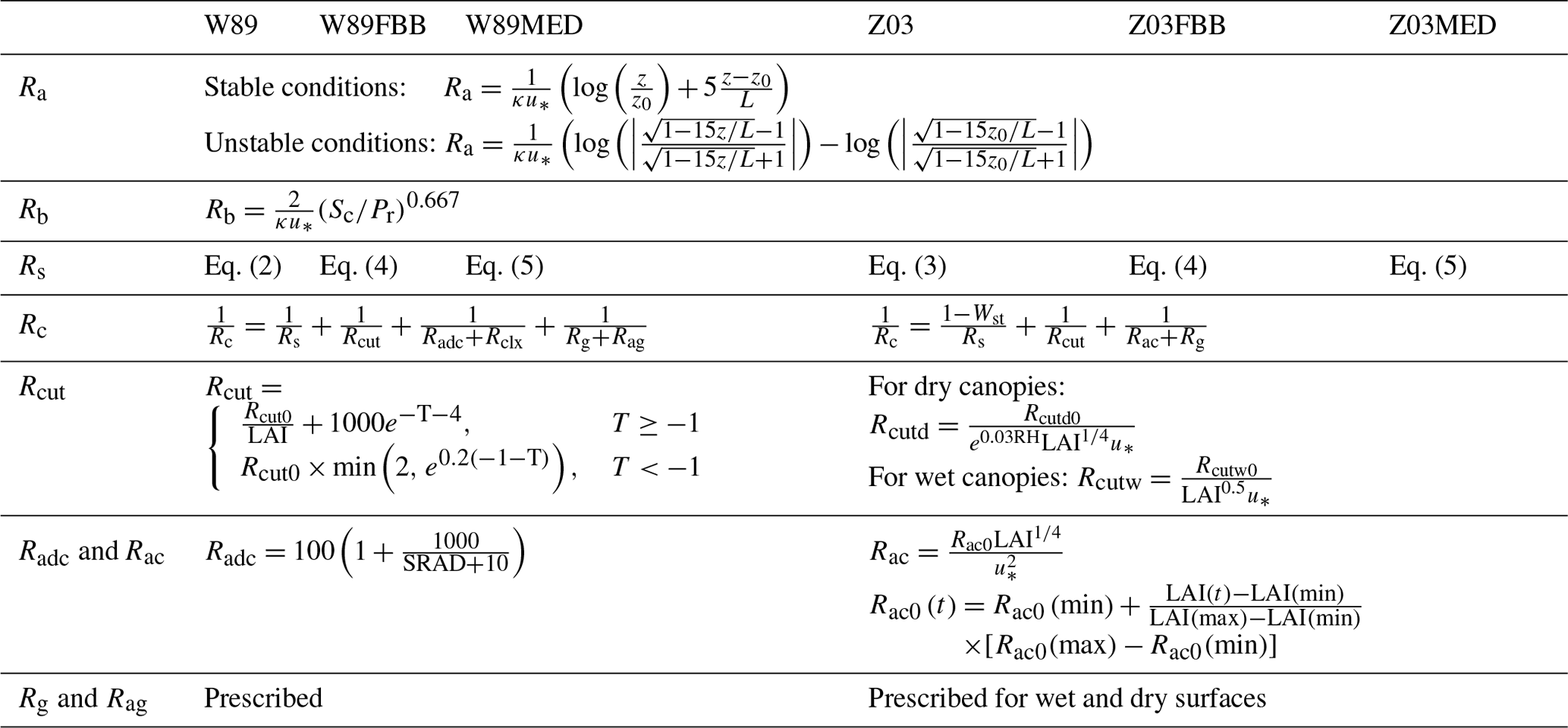
*κ: von Kármán constant; u∗: friction velocity; z0: roughness height; z: reference height; L: Obukhov length; Sr: the Schmidt number; Pr: the Prandtl number for air; LAI: leaf area index; T: surface temperature (∘C); SRAD: incoming shortwave solar radiation; Rc: canopy resistance; Rcut: cuticular resistance; Radc: lower canopy aerodynamic resistance; Rclx: lower canopy resistance; Rg: ground resistance; Rag: ground aerodynamic resistance; Rac: in-canopy aerodynamic resistance; Wst: stomatal blocking factor; RH: relative humidity; Rcutd0 and Rcutw0: reference cuticular resistance for dry and wet conditions.
In this study, we focus on comparing the different representations of Rs in dry deposition schemes. Different from the Jarvis-type algorithms commonly used in calculating dry deposition velocities, terrestrial biosphere models generally prefer the photosynthesis-based parameterization in order to calculate transpiration rate and carbon uptake. The Ball–Woodrow–Berry (BWB) model (Ball et al., 1987), which describes an empirical relationship between stomatal conductance, photosynthesis rate, RH, and leaf-surface CO2 concentration, was integrated with the Farquhar et al. (1980) photosynthesis model (collectively referred to as the Farquhar–Ball–Berry model, or FBB, hereafter) and introduced to terrestrial biosphere models in order to quantify ecosystem fluxes to and from the atmosphere starting from the mid-1990s (Sellers et al., 1996). Medlyn et al. (2011) proposed a stomatal conductance model (referred to as MED hereafter) based on the theory whereby plants optimize their stomatal behavior so as to maximize photosynthesis for given water availability (Cowan and Farquhar, 1977). MED has been parameterized with a global leaf-level gas exchange database (Lin et al., 2015) and recently implemented to replace FBB in some global land surface models (Haverd et al., 2018; Lawrence et al., 2019). The potential of implementing the optimal theory in stomatal conductance models has also been emphasized in many recent studies as they can provide a more theoretical explanation to model parameters and thus a higher predictive power under changing environments (Bai et al., 2019; Buckley et al., 2017; Katul et al., 2010; Lu et al., 2016; Sperry et al., 2017).
We examined and compared four representative stomatal schemes, including the default parameterizations in W89 and Z03, as well as two photosynthesis-based stomatal conductance (gs) modules FBB and MED. The default stomatal resistance scheme in W89 is as follows:
where Gs(LAI, PAR) represents dependence of canopy stomatal conductance on LAI and on direct and diffuse photosynthetically active radiation (PAR) within canopy as described in Wang et al. (1998). f(T) represents the temperature effects on stomatal resistance. Di and Dv are molecular diffusivities for water and the pollutant gas respectively. Details of Eq. (2) are described in Supplement Text S2. The default Z03 stomatal resistance scheme follows a two-big-leaf canopy resistance model developed by Hicks et al. (1987):
where Gs(LAI, PAR) represents unstressed total canopy stomatal conductance calculated by summing the contribution from sunlit and shaded leaves. f(T), f(VPD), and f(ψ) are dimensionless stress functions for temperature (T), vapor pressure deficit (VPD), and water stress (ψ) respectively, as described in Brook et al. (1999). These stress functions take different forms, and their details are described in Supplement Text S2.
Both FBB and MED employ the Ball–Berry approach that links leaf photosynthesis with stomatal conductance. The FBB stomatal conductance scheme computes leaf stomatal resistance as follows:
where An is leaf net photosynthesis (µmol CO2 m−2 s−1), hs is leaf surface relative humidity, Cs is CO2 concentration at the leaf surface (µmol mol−1), and g1B is the fitted slope parameter. g0 is plant functional type (PFT)-dependent minimum stomatal conductance (µmol CO2 m−2 s−1). The MED stomatal scheme is implemented as described in Medlyn et al. (2011):
where g1M is similar to g1B as above. The prescribed parameters g0 and g1M are from Lin et al. (2015). For MED and FBB, leaf stomatal conductance is coupled to the photosynthetic rate, calculated for sunlit and shaded leaves respectively, and then scaled up to the canopy level. Canopy stomatal conductance (Gs) is calculated as
where and are sunlit and shaded stomatal resistance respectively, Lsun and Lsha are sunlit and shaded LAI respectively, and rb is leaf boundary resistance. Details of the photosynthesis-based stomatal conductance module in TEMIR are also described in the Text S2.
To evaluate the two dry deposition frameworks and to compare the multiplicative and photosynthesis-based stomatal schemes, we replaced the default stomatal parameterization in W89 and Z03 dry deposition frameworks with FBB and MED, and in total six dry deposition configurations were tested as described in Table 1. The differences between the W89 and Z03 frameworks lie in not only stomatal parameterization, but also non-stomatal deposition structures and algorithms. For non-stomatal resistances, Z03 considers variations from meteorological (e.g., RH, u∗) and biological factors (e.g., LAI, wet or dry canopy), while W89 uses simpler representation of cuticular resistance and aerodynamic resistance (Table 1). Mechanistic non-stomatal parameterization remains challenging due to uncertainties in inferred non-stomatal deposition estimates, such as difficulties in separating non-stomatal uptake from soil uptake and in-canopy chemistry (Clifton et al., 2020a). Future evaluation of non-stomatal algorithms requires further measurements such as biogenic volatile organic compound (BVOC) emissions and soil moisture (Clifton et al., 2019).
Simulations using each dry deposition configuration were conducted in the single-site mode in TEMIR for the observational sites listed in Table S1. For most of the simulations, we used reanalyzed meteorological data from the Modern-Era Retrospective analysis for Research and Applications version 2 (MERRA-2) (Gelaro et al., 2017), which provides all the required meteorological input data for simulations. We also directly used the standard meteorological data from FLUXNET2015 dataset (Pastorello et al., 2020) to replace the default MERRA-2 data for FLUXNET observational sites. Cloud fraction and soil moisture data were provided by MERRA-2 for all sites. Observed site-specific LAI values were obtained from the references listed in Table S1. We applied regridded Moderate Resolution Imaging Spectroradiometer (MODIS) LAI for sites where site-specific LAI data were not available. For most of the soil and plant parameters required for TEMIR simulations, we used the Community Land Model version 4.5 (CLM4.5) land surface dataset (Lawrence and Chase, 2007) that provides parameters specific for different plant functional types (PFTs). CLM4.5 land types were mapped with W89 and Z03 land types as described in Table S3. For global simulations, the model was run at a spatial resolution of driven by MERRA-2 meteorology for each dry deposition configuration. vd and Gs were summed up by PFT fractions over vegetated land within each grid cell.
2.2 Field measurements
We compared our model results to the aggregated observations from 42 datasets of direct measurements of O3 flux and vd (Hardacre et al., 2015; Silva et al., 2018; Lin et al., 2019). All datasets used here were obtained with the eddy covariance (EC) method (Baldocchi et al., 1988). The observational sites we used covered five major vegetation types – deciduous broadleaf forest (DBF), evergreen needleleaf forest (ENF), crop (CRO), grass (GRA), and tropical rainforest (TRF) – and the majority of sites were concentrated in the US and Europe from short-term projects. Modeled seasonal mean vd values are evaluated against this compilation of observational datasets in the following section. A more detailed description of observational datasets and the corresponding references are also listed in the Table S1.
To further evaluate model capability in capturing diurnal vd and Gs, we investigated four long-term observational sites listed in Table 2: Harvard Forest, Hyytiälä Forest, Borden Forest, and Blodgett Forest. These four sites provided continuous EC measurements for momentum, sensible heat, latent heat, and O3 fluxes on an hourly basis for more than 5 years. Details of each long-term site and their data filtering methods are described in Text S1. Canopy stomatal conductance values at the long-term measurement sites were estimated based on the inverted Penman–Monteith method (referred to as P-M hereafter) using site-level FLUXNET meteorological measurements (Gerosa et al., 2007). Stomatal conductance of O3 was then calculated using the molecular diffusion coefficient ratio between O3 and water vapor.

To evaluate simulated Gs with different stomatal conductance algorithms on a larger spatiotemporal scale, we utilized the recent dataset of SynFlux (https://doi.org/10.5281/zenodo.1402054) that provides monthly daytime Gs calculated with the P-M method using standard micrometeorological flux measurements at 103 FLUXNET sites concentrated in the US and Europe where O3 monitoring networks are available (Ducker et al., 2018). We applied FLUXNET meteorology and MODIS LAI for simulations at FLUXNET sites. Simulated average monthly daytime Gs values during the measurement periods were compared with SynFlux Gs for each FLUXNET site. The uncertainties in Gs due to the fraction of soil evaporation in evapotranspiration measurements were restricted with filtered data as described in Ducker et al. (2018). The definition of daytime follows that in Ducker et al. (2018) (i.e., solar elevation angle above 4∘) for comparison with SynFlux Gs.
3.1 Evaluation of simulated seasonal average vd
The simulated seasonal average daytime vd using the different dry deposition schemes in Table 1 were evaluated with observations for major PFTs. We used two unbiased symmetric metrics – the normalized mean bias factor (NMBF) and normalized mean absolute error factor (NMAEF) – to evaluate different dry deposition schemes (Yu et al., 2006). Positive NMBF values are interpreted as overestimation by a factor of 1 + NMBF, while negative NMBF means underestimation by a factor of 1 − NMBF. Smaller absolute values of NMBF and NMAEF indicate better agreement with observations. Seasonal daytime mean observed and simulated vd and NMBF values are summarized for five major PFTs (DBF: deciduous broadleaf forest; ENF: evergreen needleleaf forest; CRO: crop; TRF: tropical rainforest; GRA: grass) in Table 3.
Table 3Seasonal mean and standard deviation of the observed and simulated ozone dry deposition velocity (cm s−1) (daytime: LT 06:00–18:00). DBF: deciduous broadleaf forest; ENF: evergreen needleleaf forest; CRO: crop; TRF: tropical rainforest; GRA: grass.
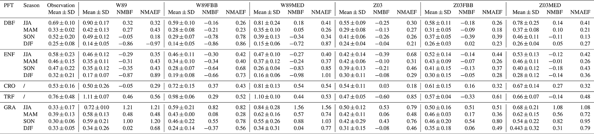
Figure 1 shows the comparison between simulated and observed daytime (06:00–18:00) average vd for five major PFTs categorized by seasons. The dry deposition schemes used in this study fit observed vd better for deciduous forest and crops. Yet different schemes cannot reproduce daytime vd well for coniferous forest, grass, and rainforest. For deciduous forests, Z03 underestimates vd in general (NMBF = −0.21; NMAEF = 0.30), while W89 overestimates vd (NMBF = 0.19; NMAEF = 0.31), with positive biases especially during summer as shown in Fig. 1a. For coniferous forests, W89 and Z03 underestimate observed vd as shown in Fig. 1b. Both W89FBB and W89MED produce higher positive biases in simulated daytime vd compared with W89 for deciduous and coniferous forests, while Z03FBB and Z03MED can reproduce observed vd with lower NMBF values than Z03. Negative biases simulated with Z03 can be caused by the prescribed maximum canopy stomatal conductance for coniferous forest, which was set lower than deciduous forest. More recent studies have observed higher unstressed maximum stomatal conductance for coniferous forest than deciduous forest (Hoshika et al., 2017). Figure 1c shows that for grasses, all dry deposition schemes overestimate vd, while Z03 and Z03FBB generally produce lower mean absolute biases (NMAEF <0.4) than other deposition schemes. In previous studies, models mostly underestimated grassland vd (Hardacre et al., 2015; Pio et al., 2000). Discrepancies between our modeled grassland vd and previous works mainly arise from the prescribed minimum stomatal resistance (rsmin) and LAI. For example, Pio et al. (2000) used rsmin (1200 s m−1) that is higher than the value (200 s m−1) we used in W89 and Z03 for grasses, resulting in lower simulated vd values than ours. In Hardacre et al. (2015), W89 underestimated vd at a long-term moorland site using rsmin (200 s m−1) and prescribed MODIS LAI, whereas in our study for the evaluation of this particular site, W89 overestimates daytime vd with positive biases of about 0.3 cm s−1 using observed LAI provided in Flechard and Fowler (1998). Observed LAI values for the observational grassland sites used in this study are higher than the grid-level MODIS LAI in the corresponding grid cell, leading to discrepancies in modeled vd.
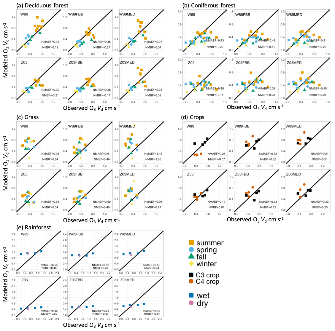
Figure 1Average daytime (LT 06:00–18:00) observed and simulated dry deposition velocities for five land types. Each data point refers to seasonal average daytime O3 dry deposition velocity from one dataset listed in Table S1. Colors indicate dominant seasons during field measurements, except for crops where different colors indicate crop types (C3 and C4 crops).
For crops as shown in Fig. 1d, Z03 better reproduces vd than the other deposition schemes with lower mean biases (NMBF = 0.01; NMAEF = 0.19). For rainforests shown in Fig. 1e, all dry deposition schemes simulate nearly constant daytime vd values for different sites, which is mainly due to the relatively uniform LAI input and meteorological conditions for tropical regions during the measurement periods. The source of discrepancies between model and observations is not clear, which can arise from various aspects such as leaf age stage of tropical trees, as well as uncertainties in the flux measurement themselves. Canopy storage effects can mask observed diurnal O3 deposition variations as previously found (Rummel et al., 2007). Current O3 flux measurements for rainforests are rather limited especially for the dry season, which also prohibits precise model parameterization (Fan et al., 1990; Sigler et al., 2002). Non-stomatal O3 deposition includes chemical reactions of O3 with nitric oxide (NO) and biogenic volatile organic compounds (BVOCs) from soil emissions (Fares et al., 2012). Recent studies have also found that in tropical rainforests, strong sources of sesquiterpenes are emitted from soil and can react rapidly with O3, contributing to non-stomatal deposition that is previously unreported (Bourtsoukidis et al., 2018).
We also compared nighttime vd simulated with different deposition schemes as shown in Fig. S1. Simulated nighttime Gs is close to zero, and thus modeled O3 dry deposition velocity mainly consists of non-stomatal sink. Field measurements have shown that non-stomatal deposition is not negligible throughout the day and that non-stomatal deposition velocity can have diurnal cycles similar to that of Gs with even higher deposition rates during the day (Hogg et al., 2007). Observed nighttime Gs is generally minimal, lower than non-stomatal conductance over vegetated regions (Caird et al., 2007; Hogg et al., 2007). W89 underestimates nighttime vd with large negative biases (NMBF < −1.4) for both deciduous and coniferous forests primarily due to underestimated non-stomatal deposition. This systematic negative bias in non-stomatal deposition can also induce misrepresentation of stomatal and non-stomatal partitioning during the day.
Overall, W89 and Z03 with multiplicative stomatal approaches produce similar biases, yet biases from Z03 are generally slightly smaller than W89 when evaluated with observations on a seasonal timescale. We found that Z03FBB generally produces lower biases, with Z03 non-stomatal parameterization and photosynthesis-based FBB stomatal conductance. Replacing the default multiplicative stomatal approach in W89 and Z03 with photosynthesis-based MED stomatal parameterization can induce higher absolute biases in simulated daytime vd.
3.2 Comparison of simulated diurnal vd at long-term measurement sites
We also evaluated simulated seasonal and diurnal vd variations using different dry deposition schemes at four long-term measurement sites listed in Table 2. Meteorological variables of temperature, relative humidity (RH), vapor pressure deficit (VPD), and root-zone soil wetness (SW) at selected sites are summarized in Table S2. Figure 2 shows observed and simulated monthly mean daytime (06:00–18:00) vd at each long-term site. The highest vd values are typically observed in summer (JJA), during which large discrepancies are also found between modeled and observed vd values. Therefore, we focused on summertime months when the highest levels of O3 concentrations and vd co-occur. W89, W89FBB, and W89MED overestimate monthly daytime vd with higher positive biases than Z03, Z03FBB, and Z03MED at Harvard Forest and Borden Forest during growing seasons. At Hyytiälä Forest, no specific scheme can better capture vd than the others. At Blodgett Forest, all dry deposition schemes underestimate vd values during JJA. We further examined simulated diurnal cycles of vd and Gs to analyze the performances of different dry deposition schemes in the following section.
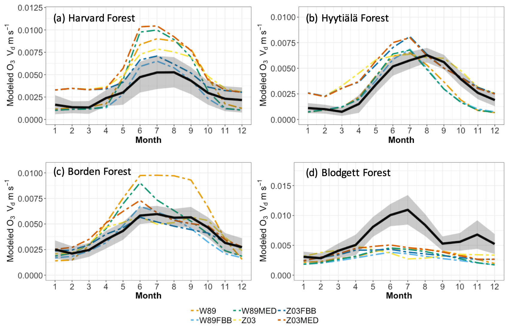
Figure 2Average monthly daytime (local time 06:00–18:00) ozone dry deposition velocity. Black solid lines indicate observed average monthly vd. Shaded envelope shows standard deviation of observed summertime average monthly daytime vd. Colored lines indicate simulated average monthly vd using different dry deposition schemes.
Figure 3 shows modeled and observed JJA diurnal vd cycles. Overall, the diurnal cycle is characterized by a sharp early morning rise in vd, followed by a gentle decline throughout the day (sometimes with a midday dip) and finally by a steeper decline toward early evening; such a typical shape strongly resembles the drawing of “a boa constrictor digesting an elephant” in the famous novella The Little Prince. Most of the schemes can capture this typical shape, with the notable exception of W89, which simply reflects a symmetric function of solar zenith angle. At Harvard Forest shown in Fig. 3a, Z03, W89FBB, and Z03FBB can well reproduce the average diurnal cycle of vd, while W89MED and Z03MED overestimate vd with early morning peaks, and W89 overestimates it with a peak shifted later in the day. Figure 4 shows the modeled and observed diurnal Gs cycles at the four sites calculated with the P-M method. As shown in Fig. 4a, overestimated vd values by W89MED and Z03MED are primarily caused by the positive biases in simulated Gs peaks during early morning and late afternoon. W89 overestimates summertime vd, which is mainly caused by overestimated afternoon Gs. Previous studies have also found that the Wesely scheme overestimated vd at Harvard Forest and assumed that the positive biases were caused by overestimated LAI from satellite observations (Hardacre et al., 2015; Silva and Heald, 2018). However, the overestimation of vd mostly arises from model parameterization as we used observed site-level LAI values in this study. Figure 5 shows the fractions of monthly average daytime stomatal conductance to canopy conductance ( and that higher fractions indicate higher ratios of stomatal deposition to non-stomatal deposition. Stomatal deposition dominates over non-stomatal deposition at Harvard Forest in summer during the day (Fig. 5). Overestimated vd at Harvard Forest is mainly caused by the stomatal parameterization, which is also emphasized in the evaluation of Gs and global simulations in the following sections of this study.
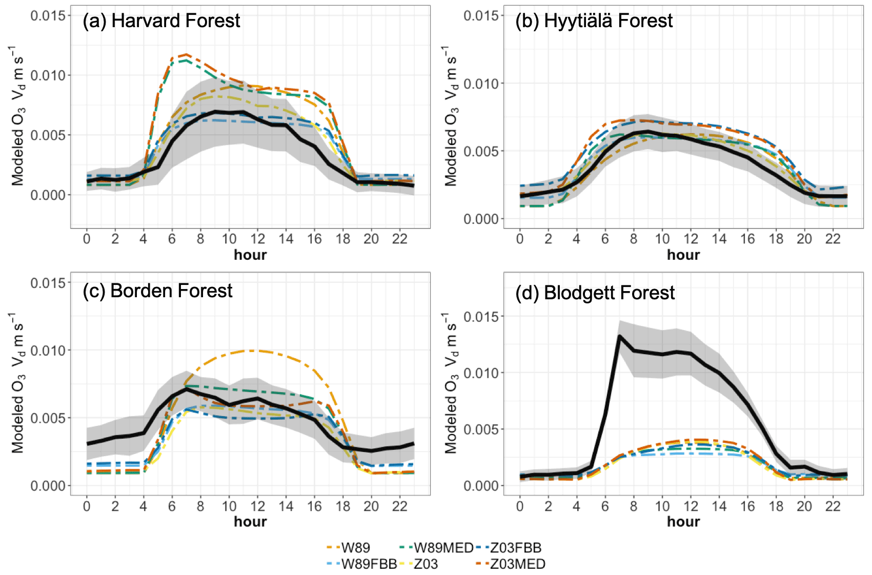
Figure 3Average diurnal cycles of ozone dry deposition velocity at four long-term observational sites. Black solid lines indicate observed average diurnal cycles of vd. Shaded envelope indicates standard deviation of summertime average hourly vd. Dashed lines indicate simulated diurnal cycles of vd using different dry deposition schemes.
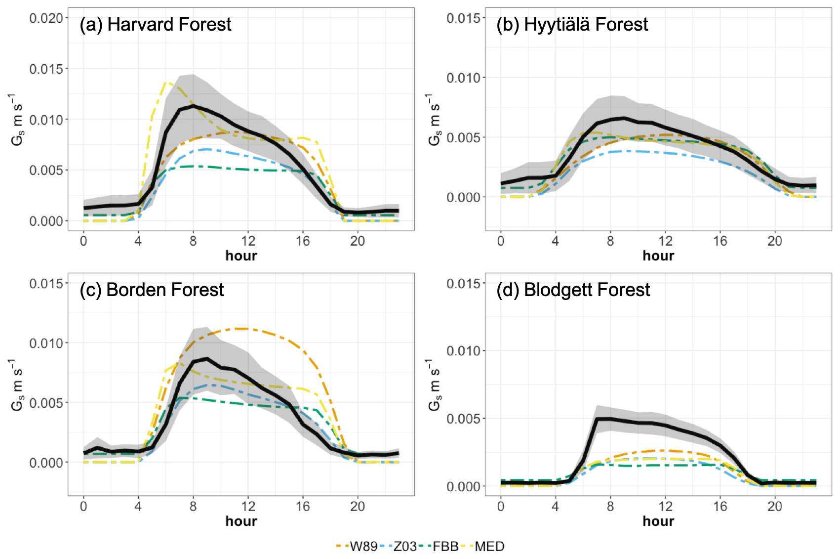
Figure 4Simulated and observed diurnal cycles of canopy stomatal conductance for ozone during summer at the four long-term measurement sites. Black lines indicate Gs derived with the P-M method. Shaded envelope shows standard deviation of summertime average hourly Gs. Colored solid lines indicate simulated stomatal conductance using multiplicative and photosynthesis-based stomatal approaches.
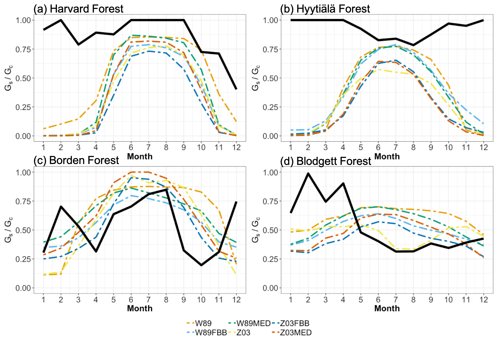
Figure 5Fractions of average monthly daytime stomatal conductance (Gs) to canopy conductance () at the four long-term measurement sites. Black lines indicate fractions calculated with Gs derived using the P-M method. Colored solid lines indicate fractions calculated with different dry deposition schemes.
The diurnal vd variations at Hyytiälä Forest can be well captured by different dry deposition schemes shown in Figure 3b. Again, W89 does not capture the typical “boa” shape. However, as shown in Figure 3d, different dry deposition schemes underestimate vd at Blodgett Forest with large negative biases despite the fact that Hyytiälä Forest and Blodgett Forest are both pine-dominated forests. The major O3 removal process in the ponderosa pine plantation at the Blodgett Ameriflux site is the non-stomatal O3 sink through in-canopy chemical reactions between O3 and BVOC (Fares et al., 2010; Kurpius and Goldstein, 2003). Rannik et al. (2012) analyzed the partitioning between stomatal and non-stomatal O3 deposition at Hyytiälä Forest, finding that O3 gas-phase chemistry is not the major contributor to O3 removal during the day. Different meteorological conditions at these two pine forest sites also result in discrepancies in simulated vd. The Blodgett Forest site is characterized by a Mediterranean climate with high surface temperature and VPD during the day for the simulation period (Table S2). Hyytiälä Forest is located in a boreal region with lower surface temperature and VPD than Blodgett Forest during summer. Previous studies have also found an exponential dependence of non-stomatal O3 deposition rates on temperature through gas-phase reactions with biogenic hydrocarbons in ponderosa pine forests (Kurpius and Goldstein, 2003). Figure 4d shows that different stomatal conductance schemes struggle to capture the magnitude of daytime stomatal O3 sink at Blodgett Forest, where water supply is limited. Besides misrepresentation of non-stomatal deposition as discussed above, underestimation of total O3 dry deposition can also be caused by not accounting for BVOC ozonolysis and non-transpiring surface deposition in dry deposition schemes.
For Borden Forest as shown in Fig. 3c, models can well capture observed vd, except that W89 overestimates vd and does not capture the typical “boa” shape. Positive biases in W89-simulated vd are mainly caused by overestimated afternoon Gs (Fig. 4c), considering that stomatal sink dominates total O3 dry deposition at Borden Forest as shown in Fig. 5c. However, underestimation of JJA vd at Borden Forest has been found in WRF-Chem simulations, which also applied the Wesely scheme (Wu et al., 2018). In our study, the W89 scheme with modification by Wang et al. (1998) applies a function for light adjustment on Rs using solar radiation and LAI, while in the Wesely scheme within WRF-Chem, LAI is not considered. It has also been argued by Wu et al. (2018) that modeled vd is largely dependent on prescribed minimum stomatal resistance (rsmin) and that uncertainties in rsmin dominate simulation errors in stomatal O3 uptake. Here we found that the inclusion of LAI in light response function can largely affect modeled stomatal conductance, leading to discrepancies in vd. Despite the fact that modifying prescribed rsmin can mitigate overall biases on a seasonal timescale, W89 still lacks the capabilities of simulating the diurnal variation of stomatal O3 uptake.
All in all, we found that stomatal parameterization can significantly affect vd simulations. The dry deposition schemes in current CTMs are parameterized in order to capture the average O3 sink over days or weeks, with less emphasis on smaller timescales such as diurnal cycles. In previous modeling works, simulated biases in vd were usually attributed to uncertainties in LAI input or coarse model resolution (Hardacre et al., 2015; Silva and Heald, 2018; Wu et al., 2018). In this study we emphasize the importance of appropriately representing diurnal vd and Gs variations in atmospheric modeling. Diurnal Gs variations and the late afternoon drop of Gs caused by the temporal lag of VPD with PAR and temperature have also been discussed in previous studies (Matheny et al., 2014; Zhang et al., 2014). W89 uses a simplified stomatal representation that is highly dependent on the variation of solar radiation and thus simulated Gs peaks with strongest sunlight despite the fact that observed diurnal Gs double peaks (the “boa” shape) when both water availability and sunlight are optimal. We found an overall overestimation of Gs by W89 especially for deciduous forest during the afternoon, which was also seen by Lei et al. (2020), resulting in positive biases in simulated vd. Z03 can better capture the observed average vd diurnal cycles than W89 mainly due to the consideration of stomatal response to VPD. Z03 considers stomatal blocking that occurs after rain or dew events and thus simulates lower dry deposition velocities at measurement sites with high precipitation. However, for most observational sites used in this study, precipitation rates are lower than the stomatal blocking threshold throughout the measurement periods, and stomatal blocking contributes little to the differences in simulated vd across different schemes. Replacing FBB stomatal parameterization in W89 can reduce biases in simulated vd cycles. In general, accounting for stomatal response to VPD and/or water stress using multiplicative or photosynthesis-based stomatal algorithms can improve model performance in capturing diurnal variations of Gs and vd.
3.3 Comparison of stomatal conductance schemes
Stomatal uptake dominates total ozone deposition during summer for long-term measurements as shown in Fig. 5. Accurate parameterization of stomatal resistance is important for not only seasonal but also diurnal courses of vd simulations. To investigate the capabilities of the four stomatal approaches, i.e., Eqs. (2) to (5), in capturing the spatial variations of Gs across four major PFTs on a global scale, we simulated Gs at 68 FLUXNET sites using different stomatal algorithms. Since no direct observations of canopy stomatal conductance or stomatal O3 flux are available, here we used SynFlux Gs derived from H2O EC fluxes with the inverted Penman–Monteith equation to evaluate different stomatal approaches (Ducker et al., 2018).
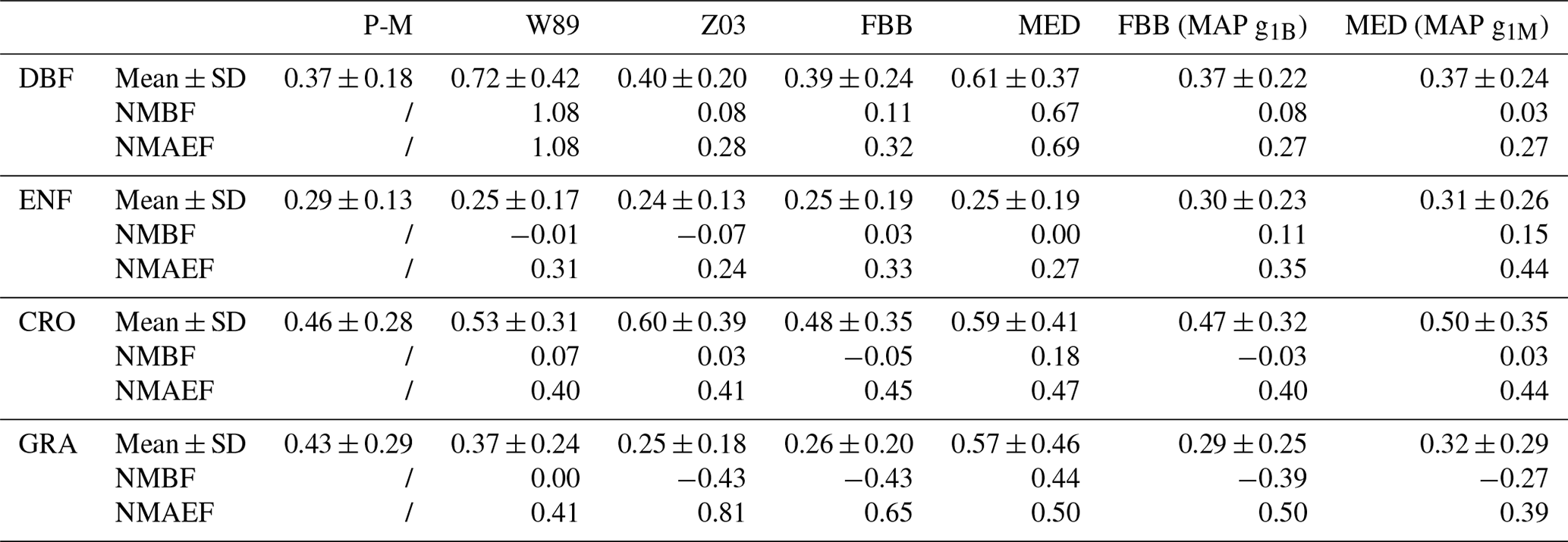
Figure 6 shows the comparison of daytime Gs during growing periods using different stomatal approaches for four major PFTs (PFT for tropical rainforest is not presented in SynFlux due to the availability of corresponding O3 measurements). The four stomatal approaches examined here can generally capture the magnitudes of Gs during the measuring periods. The multiplicative stomatal approach in Z03 simulates Gs with relatively low biases (NMBF = −0.07; NMAEF = 0.41) compared with W89, which simulates high positive biases (NMBF = 0.25; NMAEF = 0.52). Z03 and FBB produce similar biases, lower than MED or W89 in general. MED simulates Gs with higher R-squared value (R2=0.29) than other stomatal approaches (R2≤0.18). Statistic summary of monthly daytime Gs for each PFT is presented in Table 4. Different stomatal schemes simulate daytime Gs within ± 1 standard deviation evaluated using P-M Gs for major PFTs. For deciduous broadleaf forests, W89 simulates daytime Gs with the highest positive mean biases (NMBF = 1.03), while Z03 has relatively low biases (NMBF = 0.08). For the two photosynthesis-based stomatal approaches, FBB produces lower mean biases (NMBF = 0.11) than MED (NMBF = 0.67). For evergreen needleleaf forests and crops, the four stomatal algorithms can well reproduce P-M Gs, with |NMBF and |NMBF, respectively. For grasses, Z03 and FBB underestimate Gs (NMBF = −0.43), while MED overestimates Gs (NMBF = 0.44), and W89 simulates with NMAEF = 0.41, lower than other schemes (NMAEF > 0.50). Evaluation with long-term measurements in Sect. 3.2 finds similar model performance using different stomatal schemes. As shown in Fig. 4a and c, Z03 and FBB simulate comparable diurnal Gs cycles, and MED produces higher Gs values than FBB in general.
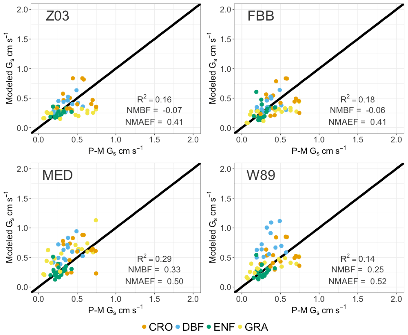
Figure 6Simulated and SynFlux daytime average canopy stomatal conductance (Gs) during growing seasons. Each point indicates daytime Gs averaged over the growing seasons for the major PFT at one FLUXNET site.
Table 4Statistic summary of monthly average daytime canopy stomatal conductance with 2 standard deviations (cm s−1). DBF: deciduous broadleaf forest; ENF: evergreen needleleaf forest; CRO: crop; GRA: grass.
Overestimated Gs using MED indicates systematic biases that can be associated with the prescribed slope parameters g1M. The predictive strengths of FBB and MED are proved to be equal in previous studies when prescribed slope parameters g1M (Eq. 5) and g1B (Eq. 4) were fitted to leaf gas exchange measurements of dominant tree species (Franks et al., 2017; Franks et al., 2018). g1M and g1B were inferred from leaf-scale gas exchange measurements that might have spatial and temporal sampling biases (Lin et al., 2015). These sampling biases were found to be reduced by inferring g1B and g1M on the canopy scale using long-term EC measurements (Knauer et al., 2018). Medlyn et al. (2017) also found that the g1M values estimated from leaf-scale and canopy-scale measurements are not consistent across PFTs and that using g1M derived from leaf-scale data can induce biases in canopy-scale simulations. Franks et al. (2018) proposed an approach for estimating the slope parameters based on the observed linear relationship between mean annual precipitation (MAP) and the slope parameters g1M and g1B. Parameterizing g1M and g1B with global MAP data can overcome the limitation of lacking spatiotemporal variations in current leaf-scale measurements, but it needs further validation with global observations. We therefore also tested MAP-derived g1B and g1M with the fitted functions described in Franks et al. (2018).
Figure 7 shows the comparison between simulated Gs using MAP-derived slope parameters and P-M-derived Gs from SynFlux. The overall biases in simulated Gs are reduced using MAP-derived g1B and g1M compared with that using PFT-specific g1B and g1M. Figure 8 shows comparison of simulated average daytime Gs using MAP-derived g1B and g1M grouped for major PFTs. The simulated Gs values using MAP-derived g1B and g1M are also summarized in Table 4 to compare with those using PFT-specific parameters. Both FBB and MED using MAP-derived g1B and g1M can reproduce Gs comparable with P-M-derived Gs across different PFTs. The positive biases in MED-simulated Gs for DBF, CRO, and GRA are reduced by using MAP-derived g1M. MED-simulated Gs that uses MAP as predictors of regional mean g1M is in better agreement with P-M Gs than that using PFT-specific g1M on the leaf scale. In previous studies, FBB and MED had equal predictive strengths when parameterized with site-specific leaf-scale data (Franks et al., 2018; Knauer et al., 2015). Our results also show that FBB and MED have comparable predictive strength when using MAP-derived g1B and g1M.
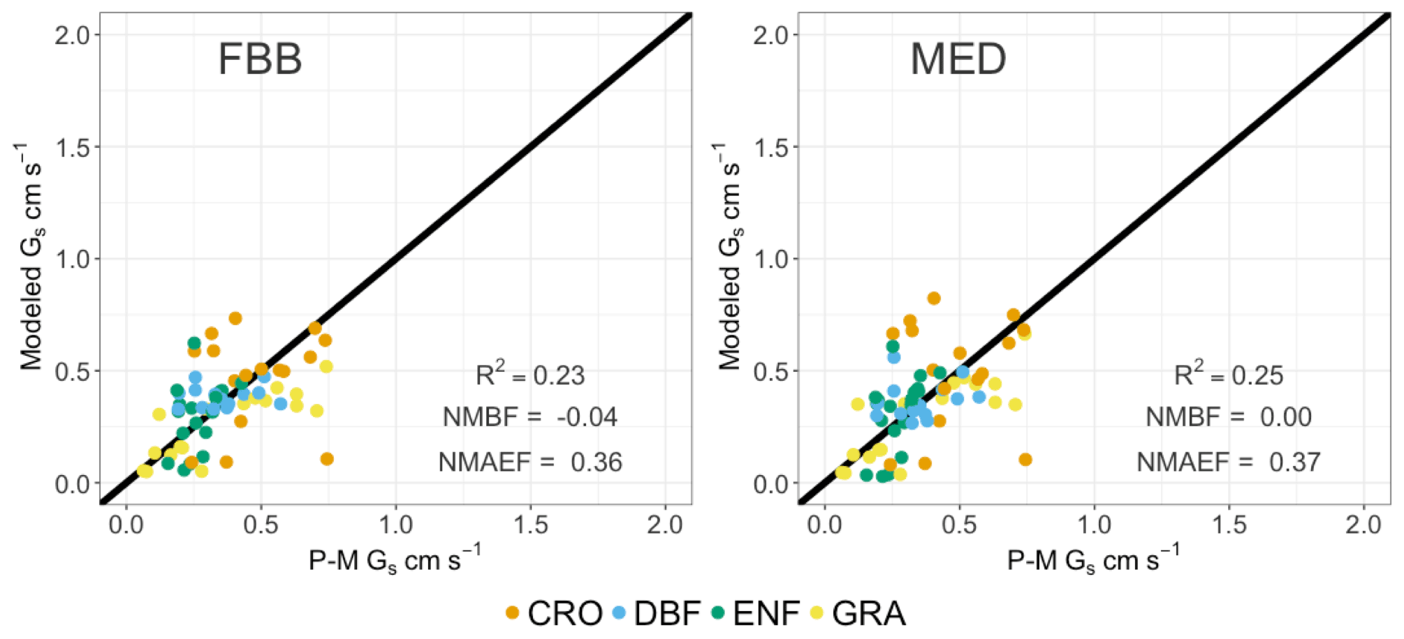
Figure 7FBB and MED using g1B and g1M derived from mean annual precipitation data compared with SynFlux canopy stomatal conductance (Gs) during growing seasons. Each point indicates average daytime Gs for the major PFT at an individual FLUXNET site.
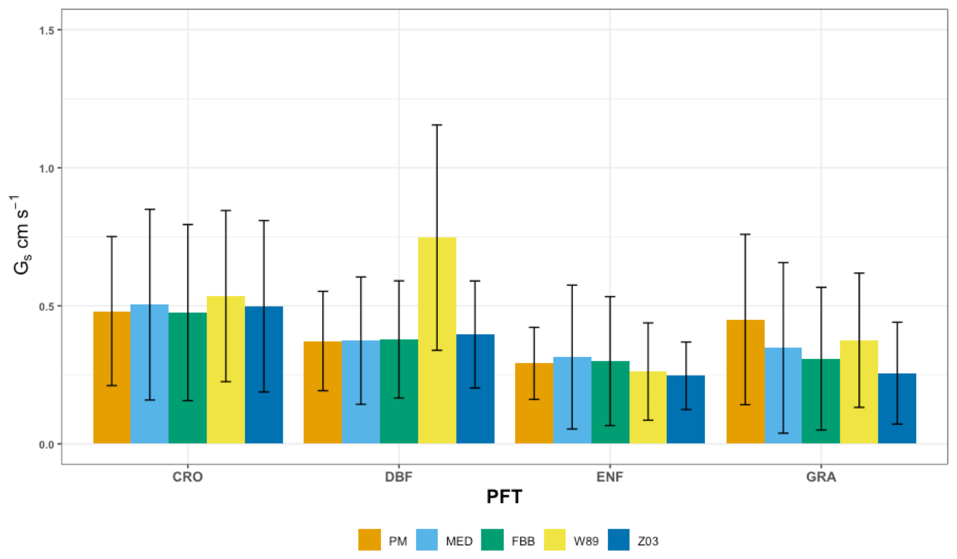
Figure 8Average daytime canopy stomatal conductance (Gs) computed with different stomatal conductance approaches for the four major PFTs. The error bars indicate 2 standard deviations. DBF: deciduous broadleaf forest; ENF: evergreen needleleaf forest; CRO: crop; GRA: grass.
In general, Jarvis-type multiplicative and photosynthesis-based stomatal approaches have comparable capabilities in reproducing the average inferred Gs from SynFlux for major vegetation types. The Jarvis-type stomatal parameterization in Z03 produces similar biases in Gs as that using FBB as shown in Table 4. MED produces higher Gs values than FBB with PFT-specific slope parameters in most cases. When using MAP-derived slope parameters, FBB and MED have similar predictive strengths. The simplified stomatal approach in W89 is unable to capture the diurnal Gs variations well without the stomatal response to water stress, and systematic positive biases in Gs are found using W89 especially for deciduous forests. The overestimated daytime Gs simulated with W89 for deciduous forest during growing seasons (Fig. 8) is also consistent with the overestimated daytime vd for deciduous forest in JJA as shown in Table 3. Therefore, the positive biases in daytime vd for deciduous forest are likely to be caused by the simplified representation of stomatal resistance in W89.
3.4 Global simulations of vd and Gs
We compared the global distribution of daytime vd and Gs simulated with the six dry deposition schemes. Simulated average July daytime vd and Gs for year 2010 to 2014 with different model configurations were compared under different CO2 levels. Ambient CO2 concentrations at 390 ppm represent the current CO2 level. For all global simulations in this section, we used MERRA-2 meteorology and MODIS LAI with a spatial resolution of . Simulated daytime vd and Gs for each grid were summed up by PFT fractions over vegetated land. Here we focus on the Northern Hemisphere where high surface O3 concentrations are typically observed during July.
Figure 9 shows July mean daytime vd during 2010–2014 over vegetated regions simulated with the six dry deposition schemes. Z03 simulates lower daytime vd than W89 in most regions, except for evergreen needleleaf regions at high latitudes (Fig. 10a), where Z03 simulates higher stomatal deposition than W89 (Fig. 11e). Hence differences in daytime vd for these regions are caused by higher non-stomatal deposition simulated by Z03. W89FBB produces higher daytime vd for evergreen needleleaf regions but lower daytime vd for deciduous broadleaf regions compared with W89 (Fig. 10b). Our evaluation results in Sect. 3.1 show that W89 overestimates observed daytime vd for deciduous broadleaf forests but underestimates vd for evergreen needleleaf forests (Fig. 1). W89FBB and Z03 can potentially better capture observed vd than W89 in global simulations especially for evergreen needleleaf and deciduous broadleaf regions.
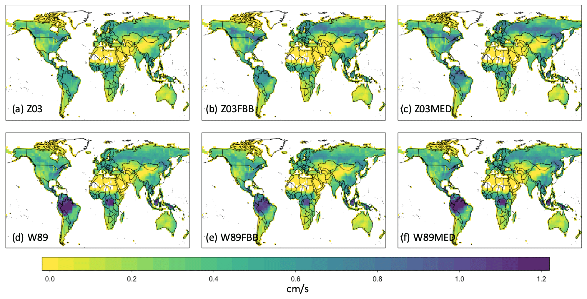
Figure 9The 2010–2014 July average daytime vd under 390 ppm CO2 level simulated with the six dry deposition schemes: (a) Z03, (b) Z03FBB, (c) Z03MED, (d) W89, (e) W89FBB, and (f) W89MED.
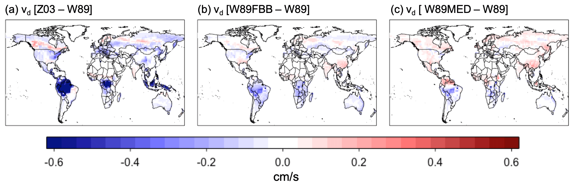
Figure 10Differences in average daytime vd between different dry deposition schemes for 2010–2014 July.
Figure 11 shows simulated July daytime Gs and the differences in simulated Gs between different stomatal approaches. Z03 simulates lower Gs than W89 in general, except for some tropical regions dominated with C4 grasses as well as some C3 crop regions in the Northern Hemisphere (Fig. 11e). Z03 also produces lower Gs than FBB, except for some regions dominated with C4 grasses (Fig. 11g). Z03 produces the lowest Gs for evergreen broadleaf forests in the tropical regions and potentially underestimates Gs in these regions, which is also found by Wong et al. (2019). The multiplicative stomatal parameterization in Z03 simulates the lowest Gs values compared with FBB, MED, and W89 for most regions. Z03 is developed for a regional air quality model focusing on North America and especially Canada and has not been evaluated with tropical forest observations, leading to potential biases for tropical regions. The slope parameters g1B and g1M in FBB and MED for C4 species are lower than those for C3 species according to the higher water use efficiency of C4 species. However, C3 and C4 photosynthesis pathways are not differentiated in Jarvis-type stomatal approaches, and this simplification in PFT classification can cause biases in Gs simulated by W89 and Z03. MED produces higher Gs than FBB (Fig. 11h) primarily due to the prescribed slope parameters as discussed in Sect. 3.3.
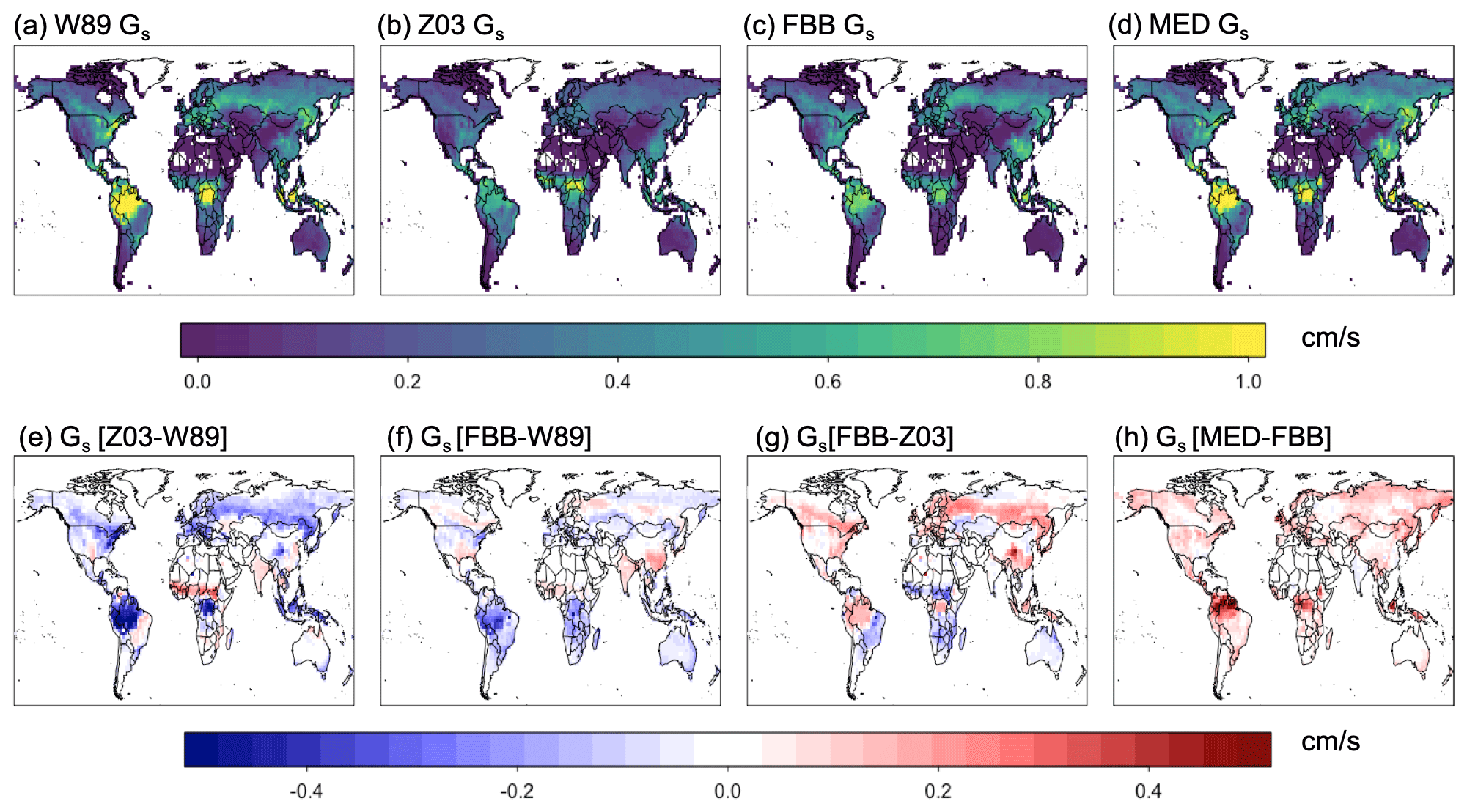
Figure 11Simulated average daytime Gs with different stomatal schemes for 2010–2014 July.
3.5 Sensitivity of stomatal conductance parameterization to elevated CO2
To test the changes in O3 dry deposition velocity due to stomatal conductance closure alone under rising CO2 levels, we conducted simulations with only variations in the choice of stomatal algorithms. Prescribed present-day meteorology and land use were applied for all simulations. Differences in simulated Gs between photosynthesis-based and multiplicative stomatal parameterization were compared. We also conducted experiments with ambient CO2 concentrations at 550 ppm and 1370 ppm, which represent future CO2 levels under RCP8.5 scenarios in 2050 and 2100 respectively. The stomatal approaches used in current LSMs are developed for short-term stomatal responses and are assumed to be adequate for long-term responses by accounting for the CO2 effect on stomatal conductance via the FBB model. Jarvis-type multiplicative schemes do not generally represent any ecophysiological responses to rising CO2, so we added an empirical CO2 response function derived from photosynthesis-based stomatal conductance model. Franks et al. (2013) summarized and tested a generalized formulation for long-term net CO2 assimilation rate (An) vs. atmospheric CO2 concentration (ca) as follows:
where An(rel) is the relative change in An, ca0 is the reference atmospheric CO2 concentration, and Γ∗ is the CO2 compensation point without dark respiration. This expression for An(rel) is based on the assumption of optimized RuBP (ribulose 1,5-bisphosphate) regeneration-limited photosynthesis in a nitrogen-limited system. The relative change in stomatal conductance is accordingly described as
where gw(rel) and ca(rel) are leaf stomatal conductance and atmospheric CO2 concentration, respectively, relative to the value in a similar system at constant current ambient CO2 concentration. We therefore applied Eqs. (7) and (8), multiplying Eq. (8) to Gs, to represent stomatal response to CO2 changes in the Jarvis-type approaches. Here we focus on the differences in simulated stomatal response to CO2 levels alone on a global scale between photosynthesis-based and Jarvis-type stomatal parameterization.
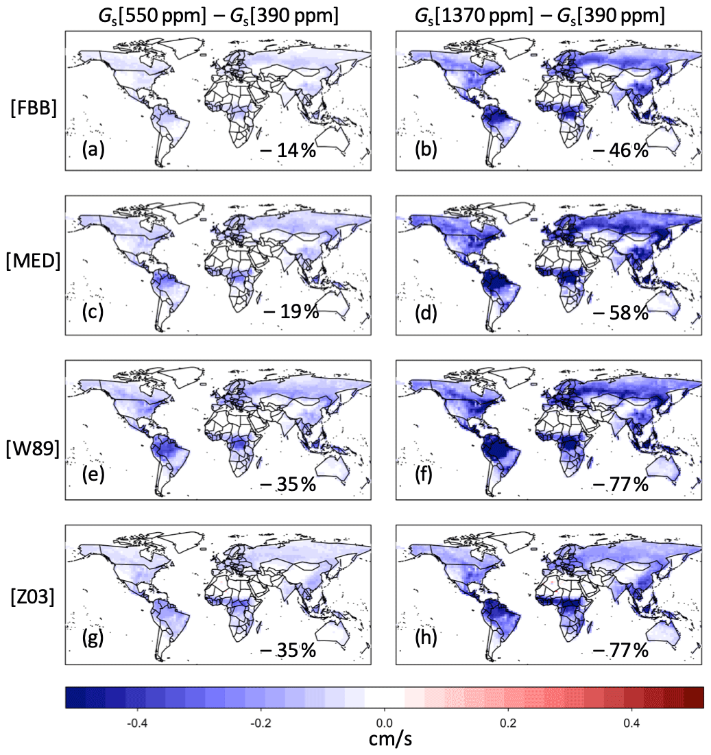
Figure 12Changes in July daytime average Gs simulated with FBB, MED, and W89 (using empirical CO2 response function) under different CO2 levels.
Figure 12 shows the changes of simulated Gs using multiplicative and photosynthesis-based stomatal approaches under different CO2 levels. Comparison of simulated Gs between 550 and 390 ppm CO2 levels is shown in the left panel of Fig. 12. The average July daytime Gs values under 550 ppm CO2 simulated with FBB and MED are reduced 14 % and 19 % respectively compared with current CO2 level, lower than the relative change of −35 % using the Jarvis-type scheme with empirical response function (Fig. 12e). Comparison of simulated Gs between 1370 ppm and 390 ppm CO2 levels is shown in the right panel of Fig. 12. FBB and MED simulate −46 % and −58 % reduction respectively in average daytime Gs, while using the Jarvis-type scheme with empirical response function gives −77 % reduction in average daytime Gs. The global average Gs computed with FBB and MED is generally less sensitive to CO2 changes than the empirical long-term response function. Simulated Gs with MED is more sensitive to elevated CO2 concentrations than FBB due to the prescribed g1M values. The long-term forest tree Free-Air CO2 Enrichment (FACE) experiments have found reductions in Gs of ∼ 20 % on average under the 550 ppm CO2 level (Ainsworth and Long, 2005), which is more consistent with what we found using the photosynthesis-based schemes than the multiplicative scheme. Yet, the magnitude of reductions in Gs varies across studies, ranging about 10 %–39 % (Herrick et al., 2004; Tricker et al., 2009; Warren et al., 2011). Using the empirical CO2 response function in Jarvis-type stomatal approaches gives a more sensitive response to elevated CO2 levels than photosynthesis-based approaches. Previous studies have found that terrestrial biosphere models using photosynthesis-based stomatal approaches combined with mechanistic parameterization of nitrogen limitation can better reproduce observed responses to CO2 enrichment experiments (Lawrence et al., 2019; Wieder et al., 2019). The Jarvis-type multiplicative stomatal approach without more mechanistic representation of complex ecophysiological constraints (e.g., nitrogen limitation, ozone damage) would likely exaggerate stomatal closure effects with higher simulated reductions in Gs under rising CO2 levels in future predictions.
This study provides an intercomparison and evaluation of dry deposition schemes, with highlights on the choice of stomatal parameterization and the importance of representing ecophysiological processes in atmospheric models. Different dry deposition and stomatal conductance schemes were implemented in a terrestrial biosphere model driven by consistent prescribed meteorological fields and land cover data to isolate the impacts of choices of model parameterization. We evaluated the most widely used dry deposition schemes against globally distributed observations. We also compared and evaluated the state-of-the-art photosynthesis-based stomatal conductance algorithms using FLUXNET measurements. Our analysis shows the importance of advancing the treatment of stomatal conductance in dry deposition schemes within current CTMs, which is essential for modeling O3 air quality under climate change, especially in relation to plant responses to water stress.
All the tested dry deposition schemes in this study can generally capture the observed seasonal average vd for major PFTs. Multiplicative W89 and Z03 reproduce observed seasonal vd with similar mean and absolute biases. Z03FBB, consisting of the photosynthesis-based FBB stomatal approach and Z03 non-stomatal parameterization, generally performs better in capturing observed seasonal daytime vd. Z03 can better simulate diurnal vd variations than W89 and can also capture observed Gs with similar mean biases as FBB for major PFTs on different timescales. W89 was parameterized to capture average vd over weeks in the early generation of CTMs and was guaranteed to reproduce seasonal observations well. Therefore, the stomatal resistance in W89 was parameterized rather simply to simulate the magnitude of observed stomatal resistance averaged over weeks accordingly (Wesely, 1989). The major difference between Z03 and W89 in the stomatal resistance calculation is whether a VPD response function is included. The misrepresentation of diurnal vd variations due to lack of water stress response in W89 can potentially cause higher biases in the simulated O3 sink since the covariation of surface O3 and stomatal conductance is based on an hourly or even half hourly timescale. The Wesely scheme in current CTMs should urgently be revised for present-day simulations to better capture diurnal variations and plant responses to water stress, which was also recommended in previous studies (Emmerichs et al., 2020; Lin et al., 2019; Niyogi et al., 1998). Despite the fact that adding a biospheric module with photosynthesis-based stomatal schemes may have additional computational cost (Lei et al., 2020), having a photosynthesis-based stomatal scheme or fully coupling dry deposition simulation in CTMs with a biosphere model would be the preferred approach for projecting future O3 air quality under changing CO2 concentration and climate. The non-stomatal parameterization in both W89 and Z03 should also be updated to better reflect our current understanding of non-stomatal sinks (Clifton et al., 2020).
The MED scheme based on the optimization stomatal theory with PFT-specific slope parameters from Lin et al. (2015) may overestimate Gs. We found that using the revised slope parameters may mitigate the high biases in simulated Gs, indicating the potential of using the slope parameters derived from global precipitation data. Current climate models lack the capability to predict hydroclimate variabilities accurately, making it difficult to link precipitation with the slope parameters in model simulations especially when precipitation is expected to be changing under climate change. Using PFT-specific slope parameters derived from globally distributed leaf-level measurements can also better capture the features of different plant species than using generic categories of C3 and C4 photosynthetic pathways. Gaps remain in understanding the spatiotemporal variations of the slope parameters in FBB and MED despite their critical role as the indicators of the intrinsic plant water use efficiency, regulated by species-related characteristics and environmental factors (Manzoni et al., 2011; Miner et al. 2017).
Disagreement was found in the spatial distribution of simulated vd and Gs using different dry deposition schemes, similar to that found previously by Wong et al. (2019). Differences in both stomatal and non-stomatal parameterizations cause regional disagreement especially for tropical forests. Comparing to the SynFlux-inferred Gs, we found potential overestimation of Gs for deciduous broadleaf forests by W89 and underestimation of Gs for evergreen needleleaf forests by Z03 on a global scale. As the inference of canopy-scale Gs can be improved by advances in partitioning transpiration and evaporation (Stoy et al., 2019), using ecosystem-scale measurements (e.g., FLUXNET) to calibrate stomatal schemes can help to overcome the limitation of leaf-level measurements in spatiotemporal coverage.
The impacts of increasing atmospheric CO2 on the terrestrial carbon sink is of great importance for land surface and climate modeling (Fatichi et al., 2019; Wieder et al., 2019). However, large uncertainties remain in the prediction of stomatal responses to climate change. The short-term variability in simulated leaf-level stomatal conductance under elevated CO2 levels mainly depends on meteorological conditions, while model parameters are more dominant in longer timescales, and thus stomatal conductance parameterization is of great importance in determining land–atmosphere interactions under future scenarios (Paschalis et al., 2017). Multiplicative and photosynthesis-based stomatal schemes simulate different sensitivities of stomatal conductance to rising CO2 concentrations. Our attempt to include the empirical CO2 response function of Franks et al. (2013) in multiplicative stomatal schemes results in a much larger reduction in global Gs that doubled the average relative change computed with photosynthesis-based stomatal schemes and potentially overstates stomatal responses to elevated CO2 under future scenarios.
In general, for atmospheric model development endeavoring to better simulate biosphere–atmosphere fluxes relevant for atmospheric chemistry, accounting for plant photosynthetic processes and other ecophysiological responses to varying environmental conditions is important especially for future predictions under changing climate and atmospheric composition. For present-day simulations of dry deposition, despite the overall performance of different deposition schemes being similar, PFT-specific or region-specific projections have large discrepancies due to different stomatal and non-stomatal parameterization. Long-term field measurements that provide hourly flux observations for major vegetation types will benefit not only stomatal and non-stomatal parameterization from diurnal to seasonal timescales, but also ecophysiological representation in atmospheric models at large, with potential to improve modeled air quality forecasts.
The TEMIR model codes are available at https://doi.org/10.5281/zenodo.6380828 (Tai et al., 2022).
The observed dry deposition datasets used in the study are listed in the references and Supplement and are available on request from the authors. The SynFlux dataset is available at https://doi.org/10.5281/zenodo.1402054 (Holmes and Ducker, 2018).
The supplement related to this article is available online at: https://doi.org/10.5194/bg-19-1753-2022-supplement.
APKT conceived the study. APKT developed the TEMIR model, and SS, DHYY, and AYHW developed additional model codes for this study. JAD and CDH provided SynFlux data. SS performed the simulations and analysis. SS and APKT prepared the paper with contributions from all co-authors.
The contact author has declared that neither they nor their co-authors have any competing interests.
Publisher's note: Copernicus Publications remains neutral with regard to jurisdictional claims in published maps and institutional affiliations.
We would like to thank Olivia E. Clifton and Sam J. Silva for providing data and advice.
This research was supported by the General Research Fund (grant no. 14306220) from the Research Grants Council of Hong Kong given to Amos P. K. Tai, as well as the US National Science Foundation (grant no. 1848372).
This paper was edited by Alexey V. Eliseev and reviewed by two anonymous referees.
Ainsworth, E. A. and Long, S. P.: What have we learned from 15 years of free-air CO2 enrichment (FACE)?, A meta-analytic review of the responses of photosynthesis, canopy, New Phytol., 165, 351–371, https://doi.org/10.1111/j.1469-8137.2004.01224.x, 2005.
Ainsworth, E. A., Yendrek, C. R., Sitch, S., Collins, W. J., and Emberson, L. D.: The Effects of Tropospheric Ozone on Net Primary Productivity and Implications for Climate Change, Annu. Rev. Plant Biol., 63, 637–661, https://doi.org/10.1146/annurev-arplant-042110-103829, 2012.
Bai, Y., Li, X. Y., Zhou, S., Yang, X. F., Yu, K. L., Wang, M. J., Liu, S. M., Wang, P., Wu, X. C., Wang, X. C., Zhang, C. C., Shi, F. Z., Wang, Y., and Wu, Y. N.: Quantifying plant transpiration and canopy conductance using eddy flux data: An underlying water use efficiency method, Agr. Forest Meteorol., 271, 375–384, https://doi.org/10.1016/j.agrformet.2019.02.035, 2019.
Baldocchi, D. D., Hicks, B. B., and Meyers, T. P.: Measuring Biosphere-Atmosphere Exchanges of Biologically Related Gases with Micrometeorological Methods, Ecology, 69, 1331–1340, https://doi.org/10.2307/1941631, 1988.
Ball, J. T., Woodrow, I. E., and Berry, J. A.: A model predicting stomatal conductance and its contribution to the control of photosynthesis under different environmental conditions, edited by: Biggins, J., in: Progress in Photosynthesis Research, Springer, Dordrecht, 221–224, https://doi.org/10.1007/978-94-017-0519-6_48, 1987.
Bey, I., Jacob, D. J., Yantosca, R. M., Logan, J. A., Field, B. D., Fiore, A. M., Li, Q. B., Liu, H. G. Y., Mickley, L. J., and Schultz, M. G.: Global modeling of tropospheric chemistry with assimilated meteorology: Model description and evaluation, J. Geophys. Res.-Atmos, 106, 23073–23095, https://doi.org/10.1029/2001JD000807, 2001.
Bonan, G. B.: Climate Change and Terrestrial Ecosystem Modeling, 1st Edn., Cambridge University Press, Cambridge, United Kingdom, https://doi.org/10.1017/9781107339217, 2019.
Bourtsoukidis, E., Behrendt, T., Yanez-Serrano, A. M., Hellen, H., Diamantopoulos, E., Catao, E., Ashworth, K., Pozzer, A., Quesada, C. A., Martins, D. L., Sa, M., Araujo, A., Brito, J., Artaxo, P., Kesselmeier, J., Lelieveld, J., and Williams, J.: Strong sesquiterpene emissions from Amazonian soils, Nat. Commun., 9, 2226, https://doi.org/10.1038/s41467-018-04658-y, 2018.
Brook, J. R., Zhang, L. M., Di-Giovanni, F., and Padro, J.: Description and evaluation of a model of deposition velocities for routine estimates of air pollutant dry deposition over North America, Part I: Model Development, Atmos. Environ., 33, 5037–5051, https://doi.org/10.1016/S1352-2310(99)00250-2, 1999.
Buckley, T. N., Sack, L., and Farquhar, G. D.: Optimal plant water economy, Plant Cell Environ., 40, 881–896, https://doi.org/10.1111/pce.12823, 2017.
Büker, P., Emberson, L. D., Ashmore, M. R., Cambridge, H. M., Jacobs, C. M. J., Massman, W. J., Muller, J., Nikolov, N., Novak, K., Oksanen, E., Schaub, M., and de la Torre, D.: Comparison of different stomatal conductance algorithms for ozone flux modelling, Environ. Pollut., 146, 726–735, https://doi.org/10.1016/j.envpol.2006.04.007, 2007.
Büker, P., Feng, Z., Uddling, J., Briolat, A., Alonso, R., Braun, S., Elvira, S., Gerosa, G., Karlsson, P. E., Le Thiec, D., Marzuoli, R., Mills, G., Oksanen, E., Wieser, G., Wilkinson, M., and Emberson, L. D.: New flux based dose-response relationships for ozone for European forest tree species, Environ. Pollut., 206, 163–174, 2015.
Byun, D. W. and Ching, J. K. S.: Science algorithms of the EPA models-3 Community Multiscale Air Quality (CMAQ) modelling system, U.S. Environmental Protection Agency, Washington, D.C., EPA/600/R-99/030 (NTIS PB2000-100561), 1999.
Caird, M. A., Richards, J. H., and Donovan, L. A.: Nighttime stomatal conductance and transpiration in C-3 and C-4 plants, Plant Physiol., 143, 4–10, https://doi.org/10.1104/pp.106.092940, 2007.
Camalier, L., Cox, W., and Dolwick, P.: The effects of meteorology on ozone in urban areas and their use in assessing ozone trends, Atmos. Environ., 41, 7127–7137, https://doi.org/10.1016/j.atmosenv.2007.04.061, 2007.
Centoni, F.: Global scale modelling of ozone deposition processes and interaction between surface ozone and climate change, Doctoral dissertation, The University of Edinburgh, https://isni.org/isni/0000000464211966 (last access: 21 March 2022), 2017.
Clifton, O. E., Fiore, A. M., Munger, J. W., and Wehr, R.: Spatiotemporal controls on observed daytime ozone deposition velocity over Northeastern U.S. forests during summer, J. Geophys. Res.-Atmos, 124, 5612–5628, https://doi.org/10.1029/2018JD029073, 2019.
Clifton, O. E., Fiore, A. M., Massman, W. J., Baublitz, C. B., Coyle, M., Emberson, L., Fares, S., Farmer, D. K., Gentine, P., Gerosa, G., Guenther, A. B., Helmig, D., Lombardozzi, D. L., Munger, J. W., Patton, E. G., Pusede, S. E., Schwede, D. B., Silva, S. J., Sorgel, M., Steiner, A. L., and Tai, A. P. K.: Dry Deposition of Ozone Over Land: Processes, Measurement, and Modeling, Rev. Geophys., 58, e2019RG000670, https://doi.org/10.1029/2019RG000670, 2020a.
Clifton, O. E., Paulot, F., Fiore, A. M., Horowitz, L. W., Correa, G., Baublitz, C. B., Fares, S., Goded, I., Goldstein, A. H., Gruening, C., Hogg, A. J., Loubet, B., Mammarella, I., Munger J. W., Neil, L., Stella, P., Uddling, J., Vesala, T., and Weng, E.: Influence of dynamic ozone dry deposition on ozone pollution, J. Geophys. Res.-Atmos, 125, e2020JD032398, https://doi.org/10.1029/2020JD032398, 2020b.
Cooper, O. R., Parrish, D. D., Ziemke, J., Balashov, N. V., Cupeiro, M., Galbally, I. E., Gilge, S., Horowitz, L., Jensen, N. R., Lamarque, J. F., Naik, V., Oltmans, S. J., Schwab, J., Shindell, D. T., Thompson, A. M., Thouret, V., Wang, Y., and Zbinden, R. M.: Global distribution and trends of tropospheric ozone: An observation-based review, Elementa, 2, 000029, https://doi.org/10.12952/journal.elementa.000029, 2014.
Cowan, I. R. and Farquhar, G. D.: Stomatal function in relation to leaf metabolism and environment, Symp. Soc. Exp. Biol., 31, 471–505, 1977.
Ducker, J. A., Holmes, C. D., Keenan, T. F., Fares, S., Goldstein, A. H., Mammarella, I., Munger, J. W., and Schnell, J.: Synthetic ozone deposition and stomatal uptake at flux tower sites, Biogeosciences, 15, 5395–5413, https://doi.org/10.5194/bg-15-5395-2018, 2018.
Elvira, S., Bermejo, V., Manrique, E., and Gimeno, B. S.: On the response of two populations of Quercus coccifera to ozone and its relationship with ozone uptake, Atmos. Environ., 38, 2305–2311, https://doi.org/10.1016/j.atmosenv.2003.10.064, 2004.
Emberson, L., Simpson, D., Tuovinen, J., Ashmore, M., and Cambridge, H.: Towards a model of ozone deposition and stomatal uptake over Europe, EMEP MSC-W Note 6/2000, EMEP MSC-W Note, 6, 1–57, 2000a.
Emberson, L., Wieser, G., and Ashmore, M.: Modelling of stomatal conductance and ozone flux of Norway spruce: comparison with field data, Environ. Poll., 109, 393–402, https://doi.org/10.1016/S0269-7491(00)00042-7, 2000b.
Emberson, L., Ashmore, M., Simpson, D., Tuovinen, J.-P., and Cambridge, H.: Modelling and mapping ozone deposition in Europe, Water Air Soil Pollut., 130, 577–582, https://doi.org/10.1023/A:1013851116524, 2001.
Emberson, L., Büker, P., and Ashmore, M.: Assessing the risk caused by ground level ozone to European forest trees: A case study in pine, beech and oak across different climate regions, Environ. Poll., 147, 454–466, https://doi.org/10.1016/j.envpol.2006.10.026, 2007.
Emmerichs, T., Kerkweg, A., Ouwersloot, H., Fares, S., Mammarella, I., and Taraborrelli, D.: A revised dry deposition scheme for land–atmosphere exchange of trace gases in ECHAM/MESSy v2.54, Geosci. Model Dev., 14, 495–519, https://doi.org/10.5194/gmd-14-495-2021, 2021.
Fan, S. M., Wofsy, S. C., Bakwin, P. S., Jacob, D. J., and Fitzjarrald, D. R.: Atmosphere-Biosphere Exchange of CO2 and O3 in the central Amazon Forest, J. Geophys. Res.-Atmos., 95, 16851–16864, https://doi.org/10.1029/JD095iD10p16851, 1990.
Fares, S., McKay, M., Holzinger, R., and Goldstein, A. H.: Ozone fluxes in a Pinus ponderosa ecosystem are dominated by non-stomatal processes: Evidence from long-term continuous measurements, Agr. Forest Meteorol., 150, 420–431, https://doi.org/10.1016/j.agrformet.2010.01.007, 2010.
Fares, S., Weber, R., Park, J.-H., Gentner, D., Karlik, J., and Goldstein, A. H.: Ozone deposition to an orange orchard: Partitioning between stomatal and non-stomatal sinks, Environ. Pollut., 169, 258–266, https://doi.org/10.1016/j.envpol.2012.01.030, 2012
Fatichi, S., Pappas, C., Zscheischler, J., and Leuzinger, S.: Modelling carbon sources and sinks in terrestrial vegetation, New Phytol., 221, 652–668, https://doi.org/10.1111/nph.15451, 2019.
Field, C. B., Jackson, R. B., and Mooney, H. A.: Stomatal responses to increased CO2: implications from the plant to the global scale, Plant Cell Environ., 18, 1214–1225, https://doi.org/10.1111/j.1365-3040.1995.tb00630.x, 1995.
Flechard, C. R. and Fowler, D.: Atmospheric ammonia at a moorland site. I: The meteorological control of ambient ammonia concentrations and the influence of local sources, Q. J. Roy. Meteor. Soc., 124, 733–757, https://doi.org/10.1002/qj.49712454705, 1998.
Fowler, D., Pilegaard, K., Sutton, M. A., Ambus, P., Raivonen, M., Duyzer, J., Simpson, D., Fagerli, H., Fuzzi, S., Schjoerring, J. K., Granier, C., Neftel, A., Isaksen, I. S. A., Laj, P., Maione, M., Monks, P. S., Burkhardt, J., Daemmgen, U., Neirynck, J., Personne, E., Wichink-Kruit, R., Butterbach-Bahl, K., Flechard, C., Tuovinen, J. P., Coyle, M., Gerosa, G., Loubet, B., Altimir, N., Gruenhage, L., Ammann, C., Cieslik, S., Paoletti, E., Mikkelsen, T. N., Ro-Poulsen, H., Cellier, P., Cape, J. N., Horvath, L., Loreto, F., Niinemets, U., Palmer, P. I., Rinne, J., Misztal, P., Nemitz, E., Nilsson, D., Pryor, S., Gallagher, M. W., Vesala, T., Skiba, U., Brueggemann, N., Zechmeister-Boltenstern, S., Williams, J., O'Dowd, C., Facchini, M. C., de Leeuw, G., Flossman, A., Chaumerliac, N., and Erisman, J. W.: Atmospheric composition change: Ecosystems-Atmosphere interactions, Atmos. Environ., 43, 5193–5267, https://doi.org/10.1016/j.atmosenv.2009.07.068, 2009.
Franks, P. J., Adams, M. A., Amthor, J. S., Barbour, M. M., Berry, J. A., Ellsworth, D. S., Farquhar, G. D., Ghannoum, O., Lloyd, J., McDowell, N., Norby, R. J., Tissue, D. T., and von Caemmerer, S.: Sensitivity of plants to changing atmospheric CO2 concentration: from the geological past to the next century, New Phytol., 197, 1077–1094, https://doi.org/10.1111/nph.12104, 2013.
Franks, P. J., Berry, J. A., Lombardozzi, D. L., and Bonan, G. B.: Stomatal Function across Temporal and Spatial Scales: Deep-Time Trends, Land-Atmosphere Coupling and Global Models, Plant Physiol., 174, 583–602, https://doi.org/10.1104/pp.17.00287, 2017.
Franks, P. J., Bonan, G. B., Berry, J. A., Lombardozzi, D. L., Holbrook, N. M., Herold, N., and Oleson, K. W.: Comparing optimal and empirical stomatal conductance models for application in Earth system models, Global Change Biol., 24, 5708–5723, https://doi.org/10.1111/gcb.14445, 2018.
Foken, T.: 50 years of the Monin-Obukhov similarity theory, Boundary-Layer Meteorol., 119, 431–447, https://doi.org/10.1007/s10546-006-9048-6, 2006.
Gelaro, R., McCarty, W., Suarez, M. J., Todling, R., Molod, A., Takacs, L., Randles, C. A., Darmenov, A., Bosilovich, M. G., Reichle, R., Wargan, K., Coy, L., Cullather, R., Draper, C., Akella, S., Buchard, V., Conaty, A., da Silva, A. M., Gu, W., Kim, G. K., Koster, R., Lucchesi, R., Merkova, D., Nielsen, J. E., Partyka, G., Pawson, S., Putman, W., Rienecker, M., Schubert, S. D., Sienkiewicz, M., and Zhao, B.: The Modern-Era Retrospective Analysis for Research and Applications, Version 2 (MERRA-2), J. Climate, 30, 5419–5454, https://doi.org/10.1175/Jcli-D-16-0758.1, 2017.
Gerosa, G., Derghi, F., and Cieslik, S.: Comparison of different algorithms for stomatal ozone flux determination from micrometeorological measurements, Water Air Soil Poll., 179, 309–321, https://doi.org/10.1007/s11270-006-9234-7, 2007.
Grell, G. A., Peckham, S. E., Schmitz, R., McKeen, S. A., Frost, G., Skamarock, W. C., and Eder, B.: Fully coupled “online” chemistry within the WRF model, Atmos. Environ., 39, 6957–6975, https://doi.org/10.1016/j.atmosenv.2005.04.027, 2005.
Hardacre, C., Wild, O., and Emberson, L.: An evaluation of ozone dry deposition in global scale chemistry climate models, Atmos. Chem. Phys., 15, 6419–6436, https://doi.org/10.5194/acp-15-6419-2015, 2015.
Haverd, V., Smith, B., Nieradzik, L., Briggs, P. R., Woodgate, W., Trudinger, C. M., Canadell, J. G., and Cuntz, M.: A new version of the CABLE land surface model (Subversion revision r4601) incorporating land use and land cover change, woody vegetation demography, and a novel optimisation-based approach to plant coordination of photosynthesis, Geosci. Model Dev., 11, 2995–3026, https://doi.org/10.5194/gmd-11-2995-2018, 2018.
Herrick, J. D., Maherali, H., and Thomas, R. B.: Reduced stomatal conductance in sweetgum (Liquidambar styraciflua) sustained over long-term CO2 enrichment, New Phytol, 162, 387–396, https://doi.org/10.1111/j.1469-8137.2004.01045.x, 2004.
Hicks, B. B., Baldocchi, D. D., Meyers, T. P., Hosker, R. P., and Matt, D. R.: A preliminary multiple resistance routine for deriving dry deposition velocities from measured quantities, Water Air Soil Poll., 36, 311–330, https://doi.org/10.1007/BF00229675, 1987.
Hogg, A., Uddling, J., Ellsworth, D., Carroll, M. A., Pressley, S., Lamb, B., and Vogel, C.: Stomatal and non-stomatal fluxes of ozone to a northern mixed hardwood forest, Tellus B, 59, 514–525, https://doi.org/10.1111/j.1600-0889.2007.00269.x, 2007.
Holmes, C. D. and Ducker, J. A.: SynFlux: a sythetic dataset of atmospheric deposition and stomatal uptake at flux tower sites (1.1), Zenodo [data set], https://doi.org/10.5281/zenodo.1402054, 2018.
Hoshika, Y., Fares, S., Savi, F., Gruening, C., Goded, I., De Marco, A., Sicard, P., and Paoletti, E.: Stomatal conductance models for ozone risk assessment at canopy level in two Mediterranean evergreen forests, Agr. Forest Meteorol., 234, 212–221, https://doi.org/10.1016/j.agrformet.2017.01.005, 2017.
Jarvis, P.: The interpretation of the variations in leaf water potential and stomatal conductance found in canopies in the field, Philos. T. Roy. Soc. B, 273, 593–610, https://doi.org/10.1098/rstb.1976.0035, 1976.
Karnosky, D. F., Skelly, J. M., Percy, K. E., and Chappelka, A. H.: Perspectives regarding 50 years of research on effects of tropospheric ozone air pollution on US forests, Environ. Pollut., 147, 489–506, https://doi.org/10.1016/j.envpol.2006.08.043, 2007.
Katul, G., Manzoni, S., Palmroth, S., and Oren, R.: A stomatal optimization theory to describe the effects of atmospheric CO2 on leaf photosynthesis and transpiration, Ann. Bot.-London, 105, 431–442, https://doi.org/10.1093/aob/mcp292, 2010.
Kavassalis, S. C. and Murphy, J. G.: Understanding ozone-meteorology correlations: A role for dry deposition, Geophys. Res. Lett., 44, 2922–2931, https://doi.org/10.1002/2016gl071791, 2017.
Keronen, P., Reissell, A., Rannik, Ü., Pohja, T., Siivola, E., Hiltunen, V., Hari, P., Kulmala, M., and Vesala, T.: Ozone flux measurements over a Scots pine forest using eddy covariance method: performance evaluation and comparison with flux-profile method, Boreal Environ. Res., 8, 425–443, 2003.
Knauer, J., Werner, C., and Zaehle, S.: Evaluating stomatal models and their atmospheric drought response in a land surface scheme: A multibiome analysis, J. Geophys. Res.-Biogeo., 120, 1894–1911, https://doi.org/10.1002/2015jg003114, 2015.
Knauer, J., Zaehle, S., Medlyn, B. E., Reichstein, M., Williams, C. A., Migliavacca, M., De Kauwe, M. G., Werner, C., Keitel, C., Kolari, P., Limousin, J. M., and Linderson, M. L.: Towards physiologically meaningful water-use efficiency estimates from eddy covariance data, Global Change Biol., 24, 694–710, https://doi.org/10.1111/gcb.13893, 2018.
Knauer, J., Zaehle, S., De Kauwe, M. G., Haverd, V., Reichstein, M., and Sun, Y.: Mesophyll conductance in land surface models: effects on photosynthesis and transpiration, Plant J., 101, 858–873, https://doi.org/10.1111/tpj.14587, 2020
Kurpius, M. R. and Goldstein, A. H.: Gas-phase chemistry dominates O3 loss to a forest, implying a source of aerosols and hydroxyl radicals to the atmosphere, Geophys. Res. Lett., 30, 1371, https://doi.org/10.1029/2002GL016785, 2003.
Lawrence, D. M., Fisher, R. A., Koven, C. D., Oleson, K. W., Swenson, S. C., Bonan, G., Collier, N., Ghimire, B., van Kampenhout, L., Kennedy, D., Kluzek, E., Lawrence, P. J., Li, F., Li, H. Y., Lombardozzi, D., Riley, W. J., Sacks, W. J., Shi, M. J., Vertenstein, M., Wieder, W. R., Xu, C. G., Ali, A. A., Badger, A. M., Bisht, G., van den Broeke, M., Brunke, M. A., Burns, S. P., Buzan, J., Clark, M., Craig, A., Dahlin, K., Drewniak, B., Fisher, J. B., Flanner, M., Fox, A. M., Gentine, P., Hoffman, F., Keppel-Aleks, G., Knox, R., Kumar, S., Lenaerts, J., Leung, L. R., Lipscomb, W. H., Lu, Y. Q., Pandey, A., Pelletier, J. D., Perket, J., Randerson, J. T., Ricciuto, D. M., Sanderson, B. M., Slater, A., Subin, Z. M., Tang, J. Y., Thomas, R. Q., Martin, M. V., and Zeng, X. B.: The Community Land Model Version 5: Description of New Features, Benchmarking, and Impact of Forcing Uncertainty, J. Adv. Model Earth Sy., 11, 4245–4287, https://doi.org/10.1029/2018MS001583, 2019.
Lawrence, P. J. and Chase, T. N.: Representing a new MODIS consistent land surface in the Community Land Model (CLM 3.0), J. Geophys. Res.-Biogeo., 112, G01023, https://doi.org/10.1029/2006jg000168, 2007.
Lei, Y., Yue, X., Liao, H., Gong, C., and Zhang, L.: Implementation of Yale Interactive terrestrial Biosphere model v1.0 into GEOS-Chem v12.0.0: a tool for biosphere–chemistry interactions, Geosci. Model Dev., 13, 1137–1153, https://doi.org/10.5194/gmd-13-1137-2020, 2020.
Lin, M. Y., Malyshev, S., Shevliakova, E., Paulot, F., Horowitz, L. W., Fares, S., Mikkelsen, T. N., and Zhang, L. M.: Sensitivity of Ozone Dry Deposition to Ecosystem-Atmosphere Interactions: A Critical Appraisal of Observations and Simulations, Global Biogeochem. Cy., 33, 1264–1288, https://doi.org/10.1029/2018gb006157, 2019.
Lin, Y. S., Medlyn, B. E., Duursma, R. A., Prentice, I. C., Wang, H., Baig, S., Eamus, D., de Dios, V. R., Mitchell, P., Ellsworth, D. S., Op de Beeck, M., Wallin, G., Uddling, J., Tarvainen, L., Linderson, M. L., Cernusak, L. A., Nippert, J. B., Ocheltree, T., Tissue, D. T., Martin-St Paul, N. K., Rogers, A., Warren, J. M., De Angelis, P., Hikosaka, K., Han, Q. M., Onoda, Y., Gimeno, T. E., Barton, C. V. M., Bennie, J., Bonal, D., Bosc, A., Low, M., Macinins-Ng, C., Rey, A., Rowland, L., Setterfield, S. A., Tausz-Posch, S., Zaragoza-Castells, J., Broadmeadow, M. S. J., Drake, J. E., Freeman, M., Ghannoum, O., Hutley, L. B., Kelly, J. W., Kikuzawa, K., Kolari, P., Koyama, K., Limousin, J. M., Meir, P., da Costa, A. C. L., Mikkelsen, T. N., Salinas, N., Sun, W., and Wingate, L.: Optimal stomatal behaviour around the world, Nat. Clim. Change, 5, 459–464, https://doi.org/10.1038/nclimate2550, 2015.
Liu, X., Tai, A. P., Chen, Y., Zhang, L., Shaddick, G., Yan, X., and Lam, H. M.: Dietary shifts can reduce premature deaths related to particulate matter pollution in China, Nat. Food, 2, 997–1004, https://doi.org/10.1038/s43016-021-00430-6, 2021.
Lombardozzi, D., Levis, S., Bonan, G., Hess, P. G., and Sparks, J. P.: The influence of chronic ozone exposure on global carbon and water cycle, J. Climate, 28, 292–305, https://doi.org/10.1175/Jcli-D-14-00223.1, 2015.
Lu, Y. J., Duursma, R. A., and Medlyn, B. E.: Optimal stomatal behaviour under stochastic rainfall, J. Theor. Biol., 394, 160–171, https://doi.org/10.1016/j.jtbi.2016.01.003, 2016.
Manzoni, S., Vico, G., Katul, G., Fay, P. A., Polley, W., Palmroth, S., and Porporato, A.: Optimizing stomatal conductance for maximum carbon gain under water stress: a meta-analysis across plant functional types and climates, Funct. Ecol., 25, 456–467, https://doi.org/10.1111/j.1365-2435.2010.01822.x, 2011.
Martin, M. V., Heald, C. L., and Arnold, S. R.: Coupling dry deposition to vegetation phenology in the Community Earth SystemModel: Implications for the simulation of surface O3, Geophys. Res. Lett., 41, 2988–2996, https://doi.org/10.1002/2014gl059651, 2014.
Matheny, A. M., Bohrer, G., Stoy, P. C., Baker, I. T., Black, A. T., Desai, A. R., Dietze, M. C., Gough, C. M., Ivanov, V. Y., Jassal, R. S., Novick, K. A., Schafer, K. V. R., and Verbeeck, H.: Characterizing the diurnal patterns of errors in the prediction of evapotranspiration by several land-surface models: An NACP analysis, J. Geophys. Res.-Biogeo., 119, 1458–1473, https://doi.org/10.1002/2014jg002623, 2014.
Medlyn, B. E., Duursma, R. A., Eamus, D., Ellsworth, D. S., Prentice, I. C., Barton, C. V. M., Crous, K. Y., de Angelis, P., Freeman, M., and Wingate, L.: Reconciling the optimal and empirical approaches to modelling stomatal conductance, Global Change Biol., 17, 2134–2144, https://doi.org/10.1111/j.1365-2486.2010.02375.x, 2011.
Medlyn, B. E., De Kauwe, M. G., Lin, Y. S., Knauer, J., Duursma, R. A., Williams, C. A., Arneth, A., Clement, R., Isaac, P., Limousin, J. M., Linderson, M. L., Meir, P., Martin-StPaul, N., and Wingate, L.: How do leaf and ecosystem measures of water-use efficiency compare?, New Phytol., 216, 758–770, https://doi.org/10.1111/nph.14626, 2017.
Meyers, T. P., Finkelstein, P., Clarke, J., Ellestad, T. G., and Sims, P. F.: A multilayer model for inferring dry deposition using standard meteorological measurements, J. Geophys. Res.-Atmos., 103, 22645–22661, https://doi.org/10.1029/98jd01564, 1998.
Mikkelsen, T. N., Ro-Poulsen, H., Pilegaard, K., Hovmand, M. F., Jensen, N. O., Christensen, C. S., and Hummelshoej, P.: Ozone uptake by an evergreen forest canopy: temporal variation and possible mechanisms, Environ. Pollut., 109, 423–429, https://doi.org/10.1016/S0269-7491(00)00045-2, 2000.
Miner, G. L., Bauerle, W. L., and Baldocchi, D. D.: Estimating the sensitivity of stomatal conductance to photosynthesis: A review, Plant Cell Environ., 40, 1214–1238, 2017.
Misson, L., Panek, J. A., and Goldstein, A. H.: A comparison of three approaches to modeling leaf gas exchange in annually drought-stressed ponderosa pine forests, Tree Physiol., 24, 529–541, https://doi.org/10.1093/treephys/24.5.529, 2004.
Monin, A. S., and Obukhov, A. M.: Basic laws of turbulent mixing in the surface layer of the atmosphere, Contrib. Geophys. Inst. Acad. Sci. USSR, 151, e187, 1954.
Monks, P. S., Archibald, A. T., Colette, A., Cooper, O., Coyle, M., Derwent, R., Fowler, D., Granier, C., Law, K. S., Mills, G. E., Stevenson, D. S., Tarasova, O., Thouret, V., von Schneidemesser, E., Sommariva, R., Wild, O., and Williams, M. L.: Tropospheric ozone and its precursors from the urban to the global scale from air quality to short-lived climate forcer, Atmos. Chem. Phys., 15, 8889–8973, https://doi.org/10.5194/acp-15-8889-2015, 2015.
Morgenstern, O., Hegglin, M. I., Rozanov, E., O'Connor, F. M., Abraham, N. L., Akiyoshi, H., Archibald, A. T., Bekki, S., Butchart, N., Chipperfield, M. P., Deushi, M., Dhomse, S. S., Garcia, R. R., Hardiman, S. C., Horowitz, L. W., Jöckel, P., Josse, B., Kinnison, D., Lin, M., Mancini, E., Manyin, M. E., Marchand, M., Marécal, V., Michou, M., Oman, L. D., Pitari, G., Plummer, D. A., Revell, L. E., Saint-Martin, D., Schofield, R., Stenke, A., Stone, K., Sudo, K., Tanaka, T. Y., Tilmes, S., Yamashita, Y., Yoshida, K., and Zeng, G.: Review of the global models used within phase 1 of the Chemistry–Climate Model Initiative (CCMI), Geosci. Model Dev., 10, 639–671, https://doi.org/10.5194/gmd-10-639-2017, 2017.
Niyogi, D., Alapaty, K., Raman, S., and Chen, F.: Development and Evaluation of a Coupled Photosynthesis-Based Gas Exchange Evapotranspiration Model (GEM) for Mesoscale Weather Forecasting Applications, J. Appl. Meteorol. Clim., 48, 349–368, https://doi.org/10.1175/2008JAMC1662.1, 2009.
Niyogi, D. S., Raman, S., and Alapaty, K.: Comparison of four different stomatal resistance schemes using FIFE data. Part II: Analysis of terrestrial biospheric-atmospheric interactions, J. Appl. Meteorol., 37, 1301–1320, https://doi.org/10.1175/1520-0450(1998)037< 1301:Cofdsr>2.0.Co;2, 1998.
Nopmongcol, U., Koo, B., Tai, E., Jung, J., Piyachaturawat, P., Emery, C., Yarwood, G., Pirovano, G., Mitsakou, C., and Kallos, G.: Modeling Europe with CAMx for the Air Quality Model Evaluation International Initiative (AQMEII), Atmos. Environ., 53, 177–185, https://doi.org/10.1016/j.atmosenv.2011.11.023, 2012.
Otu-Larbi, F.: Understanding the role of abiotic stress in biosphere-atmosphere exchange of reactive trace gases (Doctoral dissertation), Lancaster University, https://doi.org/10.17635/lancaster/thesis/1345, 2021.
Paschalis, A., Katul, G. G., Fatichi, S., Palmroth, S., and Way, D.: On the variability of the ecosystem response to elevated atmospheric CO2 across spatial and temporal scales at the Duke Forest FACE experiment, Agr. Forest Meteorol., 232, 367–383, https://doi.org/10.1016/j.agrformet.2016.09.003, 2017.
Pastorello, G., Trotta, C., Canfora, E., Chu, H., Christianson, D., Cheah, Y.-W., Poindexter, C., Chen, J., Elbashandy, A., Humphrey, M., Isaac, P., Polidori, D., Reichstein, M., Ribeca, A., van Ingen, C., Vuichard, N., Zhang, L., Amiro, B., Ammann, C., and Papale, D.: The FLUXNET2015 dataset and the ONEFlux processing pipeline for eddy covariance data, Sci. Data, 7, 225, https://doi.org/10.1038/s41597-020-0534-3, 2020.
Pio, C. A., Feliciano, M. S., Vermeulen, A. T., and Sousa, E. C.: Seasonal variability of ozone dry deposition under southern European climate conditions, in Portugal, Atmos. Environ., 34, 195–205, https://doi.org/10.1016/S1352-2310(99)00276-9, 2000.
Rannik, Ü., Altimir, N., Mammarella, I., Bäck, J., Rinne, J., Ruuskanen, T. M., Hari, P., Vesala, T., and Kulmala, M.: Ozone deposition into a boreal forest over a decade of observations: evaluating deposition partitioning and driving variables, Atmos. Chem. Phys., 12, 12165–12182, https://doi.org/10.5194/acp-12-12165-2012, 2012.
Ronan, A. C., Ducker, J. A., Schnell, J. L., and Holmes, C. D.: Have improvements in ozone air quality reduced ozone uptake into plants? Elem. Sci. Anth., 8, 2, https://doi.org/10.1525/elementa.399, 2000.
Rummel, U., Ammann, C., Kirkman, G. A., Moura, M. A. L., Foken, T., Andreae, M. O., and Meixner, F. X.: Seasonal variation of ozone deposition to a tropical rain forest in southwest Amazonia, Atmos. Chem. Phys., 7, 5415–5435, https://doi.org/10.5194/acp-7-5415-2007, 2007.
Sadiq, M., Tai, A. P. K., Lombardozzi, D., and Val Martin, M.: Effects of ozone–vegetation coupling on surface ozone air quality via biogeochemical and meteorological feedbacks, Atmos. Chem. Phys., 17, 3055–3066, https://doi.org/10.5194/acp-17-3055-2017, 2017.
Sanderson, M. G., Collins, W. J., Hemming, D. L., and Betts, R. A.: Stomatal conductance changes due to increasing carbon dioxide levels: Projected impact on surface ozone levels, Tellus B, 59, 404–411, https://doi.org/10.1111/j.1600-0889.2007.00277.x, 2007.
Schwede, D., Zhang, L. M., Vet, R., and Lear, G.: An intercomparison of the deposition models used in the CASTNET and CAPMoN networks, Atmos. Environ., 45, 1337–1346, https://doi.org/10.1016/j.atmosenv.2010.11.050, 2011.
Sellers, P. J., Randall, D. A., Collatz, G. J., Berry, J. A., Field, C. B., Dazlich, D. A., Zhang, C., Collelo, G. D., and Bounoua, L.: A revised land surface parameterization (SiB2) for atmospheric GCMs, 1. Model formulation, J. Climate, 9, 676–705, https://doi.org/10.1175/1520-0442(1996)009< 0676:Arlspf>2.0.Co;2, 1996.
Sigler, J. M., Fuentes, J. D., Heitz, R. C., Garstang, M., and Fisch, G.: Ozone dynamics and deposition processes at a deforested site in the Amazon Basin, Ambio, 31, 21–27, https://doi.org/10.1579/0044-7447-31.1.21, 2002.
Silva, S. J. and Heald, C. L.: Investigating Dry Deposition of Ozone to Vegetation, J. Geophys. Res.-Atmos., 123, 559–573, https://doi.org/10.1002/2017JD027278, 2018.
Sitch, S., Cox, P. M., Collins, W. J., and Huntingford, C.: Indirect radiative forcing of climate change through ozone effects on the land-carbon sink, Nature, 448, 791–794, https://doi.org/10.1038/nature06059, 2007.
Sperry, J. S., Venturas, M. D., Anderegg, W. R. L., Mencuccini, M., Mackay, D. S., Wang, Y. J., and Love, D. M.: Predicting stomatal responses to the environment from the optimization of photosynthetic gain and hydraulic cost, Plant Cell Environ., 40, 816–830, https://doi.org/10.1111/pce.12852, 2017.
Stevenson, D. S., Dentener, F. J., Schultz, M. G., Ellingsen, K., van Noije, T. P. C., Wild, O., Zeng, G., Amann, M., Atherton, C. S., Bell, N., Bergmann, D. J., Bey, I., Butler, T., Cofala, J., Collins, W. J., Derwent, R. G., Doherty, R. M., Drevet, J., Eskes, H. J., Fiore, A. M., Gauss, M., Hauglustaine, D. A., Horowitz, L. W., Isaksen, I. S. A., Krol, M. C., Lamarque, J. F., Lawrence, M. G., Montanaro, V., Muller, J. F., Pitari, G., Prather, M. J., Pyle, J. A., Rast, S., Rodriguez, J. M., Sanderson, M. G., Savage, N. H., Shindell, D. T., Strahan, S. E., Sudo, K., and Szopa, S.: Multimodel ensemble simulations of present-day and near-future tropospheric ozone, J. Geophys. Res.-Atmos., 111, D08301, https://doi.org/10.1029/2005jd006338, 2006.
Stoy, P. C., El-Madany, T. S., Fisher, J. B., Gentine, P., Gerken, T., Good, S. P., Klosterhalfen, A., Liu, S., Miralles, D. G., Perez-Priego, O., Rigden, A. J., Skaggs, T. H., Wohlfahrt, G., Anderson, R. G., Coenders-Gerrits, A. M. J., Jung, M., Maes, W. H., Mammarella, I., Mauder, M., Migliavacca, M., Nelson, J. A., Poyatos, R., Reichstein, M., Scott, R. L., and Wolf, S.: Reviews and syntheses: Turning the challenges of partitioning ecosystem evaporation and transpiration into opportunities, Biogeosciences, 16, 3747–3775, https://doi.org/10.5194/bg-16-3747-2019, 2019.
Szinyei, D., Gelybo, G., Guenther, A. B., Turnipseed, A. A., Toth, E., and Builtjes, P. J. H.: Evaluation of ozone deposition models over a subalpine forest in Niwot Ridge, Colorado, Idojaras, 122, 119–143, https://doi.org/10.28974/idojaras.2018.2.2, 2018.
Tai, A. P. K., Mickley, L. J., Heald, C. L., and Wu, S. L.: Effect of CO2 inhibition on biogenic isoprene emission: Implications for air quality under 2000 to 2050 changes in climate, vegetation, and land use, Geophys. Res. Lett., 40, 3479–3483, https://doi.org/10.1002/grl.50650, 2013.
Tai, A. P. K., Sadiq, M., Pang, J. Y. S., Yung, D. H. Y., and Feng, Z.: Impacts of Surface Ozone Pollution on Global Crop Yields: Comparing Different Ozone Exposure Metrics and Incorporating Co-effects of CO2, Front. Sustain. Food Syst., 5, 534616, https://doi.org/10.3389/fsufs.2021.534616, 2021.
Tai, A. P. K., Yung, D. H. Y., Pang, Y. S., and Ma, P. H. L.: amospktai/TEMIR: TEMIR v1.0 Public Release (v1.0), Zenodo [software], https://doi.org/10.5281/zenodo.6380828, 2022.
Tarasick, D., Galbally, I. E., Cooper, O. R., Schultz, M. G., Ancellet, G., Leblanc, T., Wallington, T. J., Ziemke, J., Liu, X., Steinbacher, M., Staehelin, J., Vigouroux, C., Hannigan, J. W., Garcia, O., Foret, G., Zanis, P., Weatherhead, E., Petropavlovskikh, I., Worden, H., Osman, M., Liu, J., Chang, K.-L., Gaudel, A., Lin, M., Granados-Muñoz, M., Thompson, A. M., Oltmans, S. J., Cuesta, J., Dufour, G., Thouret, V., Hassler, B., Trickl, T., and Neu, J. L.: Tropospheric Ozone Assessment Report: Tropospheric ozone from 1877 to 2016, observed levels, trends and uncertainties, Elem. Sci. Anth., 7, 72 pp., https://doi.org/10.1525/elementa.376, 2019.
Travis, K. R. and Jacob, D. J.: Systematic bias in evaluating chemical transport models with maximum daily 8 h average (MDA8) surface ozone for air quality applications: a case study with GEOS-Chem v9.02, Geosci. Model Dev., 12, 3641–3648, https://doi.org/10.5194/gmd-12-3641-2019, 2019.
Tricker, P. J., Pecchiari, M., Bunn, S. M., Vaccari, F. P., Peressotti, A., Miglietta, F., and Taylor, G.: Water use of a bioenergy plantation increases in a future high CO2 world, Biomass Bioenerg., 33, 200–208, https://doi.org/10.1016/j.biombioe.2008.05.009, 2009.
Uddling, J., Hall, M., Wallin, G., and Karlsson, P. E.: Measuring and modelling stomatal conductance and photosynthesis in mature birch in Sweden, Agr. Forest Meteorol., 132, 115–131, https://doi.org/10.1016/j.agrformet.2005.07.004, 2005.
Vingarzan, R.: A review of surface ozone background levels and trends, Atmos. Environ., 38, 3431–3442, https://doi.org/10.1016/j.atmosenv.2004.03.030, 2004.
Wang, Y. H., Jacob, D. J., and Logan, J. A.: Global simulation of tropospheric O3-NOx-hydrocarbon chemistry 1. Model formulation, J. Geophys. Res.-Atmos., 103, 10713–10725, https://doi.org/10.1029/98jd00158, 1998.
Warren, J. M., Norby, R. J., and Wullschleger, S. D.: Elevated CO2 enhances leaf senescence during extreme drought in a temperate forest, Tree Physiol., 31, 117–130, https://doi.org/10.1093/treephys/tpr002, 2011.
Wesely, M. L.: Parameterization of Surface Resistances to Gaseous Dry Deposition in Regional-Scale Numerical-Models, Atmos. Environ., 23, 1293–1304, https://doi.org/10.1016/0004-6981(89)90153-4, 1989.
Wesely, M. L. and Hicks, B. B.: A review of the current status of knowledge on dry deposition, Atmos. Environ., 34, 2261–2282, https://doi.org/10.1016/S1352-2310(99)00467-7, 2000.
Wieder, W. R., Lawrence, D. M., Fisher, R. A., Bonan, G. B., Cheng, S. J., Goodale, C. L., Grandy, A. S., Koven, C. D., Lombardozzi, D. L., Oleson, K. W., and Thomas, R. Q.: Beyond Static Benchmarking: Using Experimental Manipulations to Evaluate Land Model Assumptions, Global Biogeochem. Cy., 33, 1289–1309, https://doi.org/10.1029/2018gb006141, 2019.
Wild, O.: Modelling the global tropospheric ozone budget: exploring the variability in current models, Atmos. Chem. Phys., 7, 2643–2660, https://doi.org/10.5194/acp-7-2643-2007, 2007.
Wong, A. Y. H., Geddes, J. A., Tai, A. P. K., and Silva, S. J.: Importance of dry deposition parameterization choice in global simulations of surface ozone, Atmos. Chem. Phys., 19, 14365–14385, https://doi.org/10.5194/acp-19-14365-2019, 2019.
Wu, Z. Y., Wang, X. M., Chen, F., Turnipseed, A. A., Guenther, A. B., Niyogi, D., Charusombat, U., Xia, B. C., Munger, J. W., and Alapaty, K.: Evaluating the calculated dry deposition velocities of reactive nitrogen oxides and ozone from two community models over a temperate deciduous forest, Atmos. Environ., 45, 2663–2674, https://doi.org/10.1016/j.atmosenv.2011.02.063, 2011.
Wu, Z. Y., Schwede, D. B., Vet, R., Walker, J. T., Shaw, M., Staebler, R., and Zhang, L. M.: Evaluation and Intercomparison of Five North American Dry Deposition Algorithms at a Mixed Forest Site, J. Adv. Model Earth Sy., 10, 1571–1586, https://doi.org/10.1029/2017ms001231, 2018.
Young, P. J., Naik, V., Fiore, A. M., Gaudel, A., Guo, J., Lin, M. Y., Neu, J. L., Parrish, D. D., Rieder, H. E., Schnell, J. L., Tilmes, S., Wild, O., Zhang, L., Ziemke, J., Brandt, J., Delcloo, A., Doherty, R. M., Geels, C., Hegglin, M. I., Hu, L., Im, U., Kumar, R., Luhar, A., Murray, L., Plummer, D., Rodriguez, J., Saiz-Lopez, A., Schultz, M. G., Woodhouse, M. T., and Zeng, G.: Tropospheric Ozone Assessment Report: Assessment of global-scale model performance for global and regional ozone distributions, variability, and trends, Elem. Sci. Anth., 6, p. 10, https://doi.org/10.1525/elementa.265, 2018.
Yu, S. C., Eder, B., Dennis, R., Chu, S. H., and Schwartz, S. E.: New unbiased symmetric metrics for evaluation of air quality models, Atmos. Sci. Lett., 7, 26–34, https://doi.org/10.1002/asl.125, 2006.
Zhang, L., Vet, R., O'Brien, J. M., Mihele, C., Liang, Z., and Wiebe, A.: Dry deposition of individual nitrogen species at eight Canadian rural sites, J. Geophys. Res.-Atmos., 114, D02301, https://doi.org/10.1029/2008jd010640, 2009.
Zhang, Q., Manzoni, S., Katul, G., Porporato, A., and Yang, D. W.: The hysteretic evapotranspiration- Vapor pressure deficit relation, J. Geophys. Res.-Biogeo., 119, 125–140, https://doi.org/10.1002/2013jg002484, 2014.
Zhao, Y., Zhang, L., Tai, A. P. K., Chen, Y., and Pan, Y.: Responses of surface ozone air quality to anthropogenic nitrogen deposition in the Northern Hemisphere, Atmos. Chem. Phys., 17, 9781–9796, https://doi.org/10.5194/acp-17-9781-2017, 2017.
Zhou, S. S., Tai, A. P. K., Sun, S., Sadiq, M., Heald, C. L., and Geddes, J. A.: Coupling between surface ozone and leaf area index in a chemical transport model: strength of feedback and implications for ozone air quality and vegetation health, Atmos. Chem. Phys., 18, 14133–14148, https://doi.org/10.5194/acp-18-14133-2018, 2018.
Zhu, J., Tai, A. P. K., and Hung Lam Yim, S.: Effects of ozone–vegetation interactions on meteorology and air quality in China using a two-way coupled land–atmosphere model, Atmos. Chem. Phys., 22, 765–782, https://doi.org/10.5194/acp-22-765-2022, 2022.
Zhu, Z. C., Piao, S. L., Myneni, R. B., Huang, M. T., Zeng, Z. Z., Canadell, J. G., Ciais, P., Sitch, S., Friedlingstein, P., Arneth, A., Cao, C. X., Cheng, L., Kato, E., Koven, C., Li, Y., Lian, X., Liu, Y. W., Liu, R. G., Mao, J. F., Pan, Y. Z., Peng, S. S., Penuelas, J., Poulter, B., Pugh, T. A. M., Stocker, B. D., Viovy, N., Wang, X. H., Wang, Y. P., Xiao, Z. Q., Yang, H., Zaehle, S., and Zeng, N.: Greening of the Earth and its drivers, Nat. Clim. Change, 6, 791, https://doi.org/10.1038/nclimate3004, 2016.