the Creative Commons Attribution 4.0 License.
the Creative Commons Attribution 4.0 License.
 | 31 Mar 2022
A convolutional neural network for spatial downscaling of satellite-based solar-induced chlorophyll fluorescence (SIFnet)
Johannes Gensheimer
Philipp Köhler
Christian Frankenberg
Gross primary productivity (GPP) is the sum of leaf photosynthesis and represents a crucial component of the global carbon cycle. Space-borne estimates of GPP typically rely on observable quantities that co-vary with GPP such as vegetation indices using reflectance measurements (e.g., normalized difference vegetation index, NDVI, near-infrared reflectance of terrestrial vegetation, NIRv, and kernel normalized difference vegetation index, kNDVI). Recent work has also utilized measurements of solar-induced chlorophyll fluorescence (SIF) as a proxy for GPP. However, these SIF measurements are typically coarse resolution, while many processes influencing GPP occur at fine spatial scales. Here, we develop a convolutional neural network (CNN), named SIFnet, that increases the resolution of SIF from the TROPOspheric Monitoring Instrument (TROPOMI) on board of the satellite Sentinel-5P by a factor of 10 to a spatial resolution of 500 m. SIFnet utilizes coarse SIF observations together with high-resolution auxiliary data. The auxiliary data used here may carry information related to GPP and SIF. We use training data from non-US regions between April 2018 until March 2021 and evaluate our CNN over the conterminous United States (CONUS). We show that SIFnet is able to increase the resolution of TROPOMI SIF by a factor of 10 with a r2 and RMSE metrics of 0.92 and 0.17 mW m−2 sr−1 nm−1, respectively. We further compare SIFnet against a recently developed downscaling approach and evaluate both methods against independent SIF measurements from Orbiting Carbon Observatory 2 and 3 (together OCO-2/3). SIFnet performs systematically better than the downscaling approach (r=0.78 for SIFnet, r=0.72 for downscaling), indicating that it is picking up on key features related to SIF and GPP. Examination of the feature importance in the neural network indicates a few key parameters and the spatial regions in which these parameters matter. Namely, the CNN finds low-resolution SIF data to be the most significant parameter with the NIRv vegetation index as the second most important parameter. NIRv consistently outperforms the recently proposed kNDVI vegetation index. Advantages and limitations of SIFnet are investigated and presented through a series of case studies across the United States. SIFnet represents a robust method to infer continuous, high-spatial-resolution SIF data.
- Article
(15812 KB) - Full-text XML
-
Supplement
(12518 KB) - BibTeX
- EndNote


Photosynthesis represents the single largest CO2 flux between the atmosphere and the biosphere. At the canopy level, the sum of all leaf photosynthesis is termed gross primary productivity (GPP), and accurate characterization of GPP represents a major uncertainty in the carbon cycle (Friedlingstein et al., 2019). Directly measuring GPP from remote sensing systems (e.g., satellites) is not presently possible. Instead, previous work has utilized stationary measurements of net ecosystem exchange (NEE) from flux towers that can be decomposed into GPP and respiration (e.g., Reichstein et al., 2005). Observable quantities from satellites (e.g., vegetation indices computed from reflectance data) are then related to GPP inferred from flux towers (e.g., Huete et al., 2006; Jung et al., 2019; Sims et al., 2006; Zeng et al., 2020) in light use efficiency (LUE) (Mahadevan et al., 2008) or machine learning models (Jung et al., 2019) to derive global estimates of GPP.
Vegetation indices such as the normalized difference vegetation index (NDVI) and near-infrared reflectance of terrestrial vegetation (NIRv) combine two (or more) spectral bands with different absorption characteristics (Hanes, 2013) to infer quantities related to plant physiology and canopy structure. The MODIS instrument was launched on the Terra and Aqua satellites in 1999 and 2002, respectively. This instrument has proved particularly useful due, in part, to the long operational lifetime, and vegetation indices can be derived from the individual reflectance bands of MODIS. More recently launched satellites, like Sentinel-5P, carry instruments with the necessary signal-to-noise ratio and spectral resolution to retrieve solar-induced chlorophyll fluorescence (SIF). The electromagnetic signal SIF is emitted by chlorophylls during photosynthesis. SIF is emitted in the red–far-red wavelengths of 650–850 nm (Magney et al., 2020). It is a way, besides photochemistry and nonphotochemical quenching, for de-excitement of the chlorophylls (Turner et al., 2020; Köhler et al., 2018). Even though the link between chlorophyll fluorescence and photosynthesis is nonlinear at leaf and canopy scale, that does not hold for satellite scales, in which a linear relationship of SIF to GPP is frequently reported (e.g., Turner et al., 2021; Magney et al., 2020; Frankenberg et al., 2011; Joiner et al., 2011).
Vegetation indices (also termed greenness) can be regarded as a measure of photosynthetic capacity (Sellers, 1985), whereas SIF indicates photosynthetic activity. SIF has been shown to be a powerful proxy for estimating GPP (Magney et al., 2019; Turner et al., 2021), to capture the impact of drought on photosynthetic activities across different vegetation types (Shekhar et al., 2020a; Castro et al., 2020), and to assess the regional source of carbon emissions (Shekhar et al., 2020b).
Köhler et al. (2018) described the first retrievals of SIF from the TROPOspheric Monitoring Instrument (TROPOMI), the sole instrument on the Sentinel-5P satellite. The TROPOMI instrument has an equatorial crossing time of 13:30 local solar time and a 16 d orbit cycle. TROPOMI has a wide swath (2600 km across track) that allows for near-daily temporal resolution and a spatial resolution of 5.5 × 3.5 km. This was a substantial improvement to previous satellite instruments measuring SIF that were limited to 40 × 40 km spatial resolution (Joiner et al., 2013). Despite the higher spatial resolution of TROPOMI, there have been efforts to estimate SIF at finer spatial scales (e.g., Turner et al., 2020). This is motivated by the importance of fine-scale phenomena in the carbon cycle such as ecosystem fragmentation (e.g., Haddad et al., 2015).
Globally, 20 % and 70 % of the remaining forests are within a distance of 100 m and 1 km, respectively, from the forest edges, meaning that most of the forests are fragmented (Haddad et al., 2015). Reinmann and Hutyra (2017) show that the carbon uptake and storage of trees near the forest edge increase up to 13 ± 3 % and 10 ± 1 %, respectively. On the other hand most of our understanding about forest carbon fluxes comes from intact ecosystems, resulting in a mismatch between the ecosystems we are trying to quantify and the data we are using to do so (Smith et al., 2018). Higher-resolution estimates of photosynthetic activity might enable us to include fragmentation effects of ecosystems to global carbon cycle estimates or biosphere models like Jung et al. (2019), Wu et al. (2021), and Turner et al. (2021). Additionally, recent work has shown the importance of fine-scale variations in the urban biosphere on the overall carbon flux for a city (e.g., Miller et al., 2020).
There has been some recent work with the goal of increasing the resolution of existing global SIF estimates through downscaling methods (i.e., physics-based methods). For example, Turner et al. (2020, 2021) used NIRv to partition SIF within a particular TROPOMI scene and oversampled it using a 16 d window afterwards, resulting in a daily 500 m SIF estimate over the conterminous United States (CONUS). Duveiller et al. (2020) downscaled GOME-2 satellite SIF from 0.5 to 0.05∘ using a parameterization with a term for the fraction of absorbed photosynthetically active radiation (fAPAR), one for water stress, and one for heat stress based on MODIS data. Siegmann et al. (2021) used airborne data to downscale far-red SIF from canopy to leaf level.
Machine learning has also been used to create global, high-resolution SIF data sets. Li and Xiao (2019), Yu et al. (2019), and Zhang et al. (2018) used spectral bands from MODIS as input to neural networks that were trained with Orbiting Carbon Observatory 2 (OCO-2) SIF data to build global continuous SIF products at 0.05∘ resolution. OCO-2 has a narrow swath, and, therefore, the networks are trained only in the regions where OCO-2 SIF is available by using MODIS data as input. After training, the global MODIS data are used as input to estimate SIF on a global scale. Gentine and Alemohammad (2018) use MODIS reflectance data as input and predict GOME-2 normalized by clear-sky irradiance. Multiplying that with a MODIS-derived photosynthetic active radiation product results in a MODIS only estimated SIF, termed RSIF. Zhang et al. (2021) trained a convolutional neural network (CNN) with MODIS data on the artificial GOSIF data set (Li and Xiao, 2019) at a resolution of 0.05∘ and used the trained network and MODIS data at a resolution of 0.008∘ to estimate SIF at 0.008∘. The physics-based downscaling approach from Turner et al. (2020) can only consider one variable for weighting the SIF signal, while the machine-learning-based approaches in the literature can consider more than one variable – but many do not use SIF data as an input to their model, meaning that they estimate SIF based on reflectance data.
Here we build a convolutional neural network to obtain high-resolution SIF, named SIFnet. SIFnet increases the spatial resolution of TROPOMI SIF by considering coarse-resolution SIF with high-resolution auxiliary data as input. These auxiliary data consist of either proxies of SIF or photosynthetic drivers. SIFnet is trained using data with near-global coverage. Different model parameters (structure, input features, and scaling factors) are compared and evaluated. After training the model, the resolution of TROPOMI SIF is refined by a factor of 10 to a spatial resolution of 0.005∘. This product is then compared against a recent downscaling method from the literature (Turner et al., 2020). Both high-resolution estimates are validated over CONUS against the independent SIF measurements of the OCO-2 and OCO-3 instruments (together OCO-2/3) (OCO-2 Science Team/Michael Gunson, 2020; OCO-3 Science Team/Michael Gunson, 2020).
2.1 Data sources
The input data to the neural network are listed in Table 1. These diverse global data products are expected to capture a broad range of photosynthetic drivers. The table divides the data into time-varying or time-invariant and training or validation data. The native spatial resolution is shown in the last column of Table 1. In a first step, all data sets are aggregated to 0.05∘ spatial resolution and 16 d time steps. In the case of a higher native spatial resolution, the data are regridded by computing the mean value that falls into the coarse-resolution grid cell. In the case of coarser resolutions than 0.05∘, it is resampled to the common grid. Quality control flags and cloud filtering are applied when necessary.
Table 1Data sets used in this work. ENF: evergreen needleleaf forest; EBF: evergreen broadleaf forest; DNF: deciduous needleleaf forest; DBF: deciduous broadleaf forest; MF: mixed forest; UF: unknown forest.

References: 1 Köhler et al. (2018); 2 Schaaf and Wang (2015); 3 Copernicus Climate Change Service (2017); 4 Entekhabi et al. (2010); 5 PySolar (2021); 6 Danielson and Gesch (2011); 7 Buchhorn et al. (2020); 8 Morreale et al. (2021); 9 OCO-2 Science Team/Michael Gunson (2020); 10 OCO-3 Science Team/Michael Gunson (2020).
MODIS measures the reflected radiance from the earth surface in seven different spectral bands covering the visible and infrared spectral region. Vegetation indices are computed by combining the near-infrared (where chlorophyll is non-absorbing) and the red band (where chlorophyll is highly absorbing) (Hanes, 2013). Specifically, the normalized difference vegetation index (NDVI) (Tucker, 1979), near-infrared vegetation index (NIRv) (Badgley et al., 2017), the kernel NDVI (kNDVI) (Camps-Valls et al., 2021), and the enhanced vegetation index (EVI) (Huete et al., 2002) are computed as follows:
EVI coefficients for MODIS are as follows: L=1, C1=5, C2=7.5, and G=2.5 (Huete et al., 2002). ρNIR is the near infrared band, ρRED is the red band, and ρBLUE is the blue band from the MODIS satellites.
Temperature and precipitation are taken from ERA5-Land data at the time step of interest and with a delay of one time step. Soil moisture has been shown to be a strong driver of global photosynthesis due, in part, to its impact on vapor-pressure deficit (Humphrey et al., 2021). Here we use the coarse-resolution NASA USDA Soil Moisture Active Passive (SMAP) soil moisture (Entekhabi et al., 2010) as a model input and explore its correlation with TROPOMI SIF. The cosine of the solar zenith angle (SZA) is a proxy for photosynthetically active radiation (PAR) under cloud-free conditions (Chen et al., 2020; Turner et al., 2021).
Time-invariant data sets consist of elevation data, fractional land cover classification, and forest fragmentation data. The land cover classification (Buchhorn et al., 2020) is resampled to 11 fractional classes. The forest fragmentation data consist of two bands and have a native resolution of 30 m. One band describes the share of forest within the grid cell (forest share) and the other how much of that forest is edge forest (defined as a maximum distance to an edge or other land cover type of 30 m). OCO-2 and OCO-3 have high spatial resolution (2.25 × 1.29 km) but small swaths (10 km) and a 16 d revisit time.
2.2 Covariation of input data sets with SIF
We are interested in understanding what these different data sets are telling us about SIF and also how they co-vary with each other. We compare all collected time variant data against TROPOMI SIF in the spatial and temporal domain. As a quantitative measure, we compute the Pearson correlation coefficient (r) (Benesty et al., 2009). Figure 1 shows a scatter comparison of SIF against the auxiliary data at the lowest resolution of the two corresponding sets. Negative SIF values (on the x axis in Fig. 1) are due to relatively high retrieval errors which scale with radiance levels (Köhler et al., 2018).
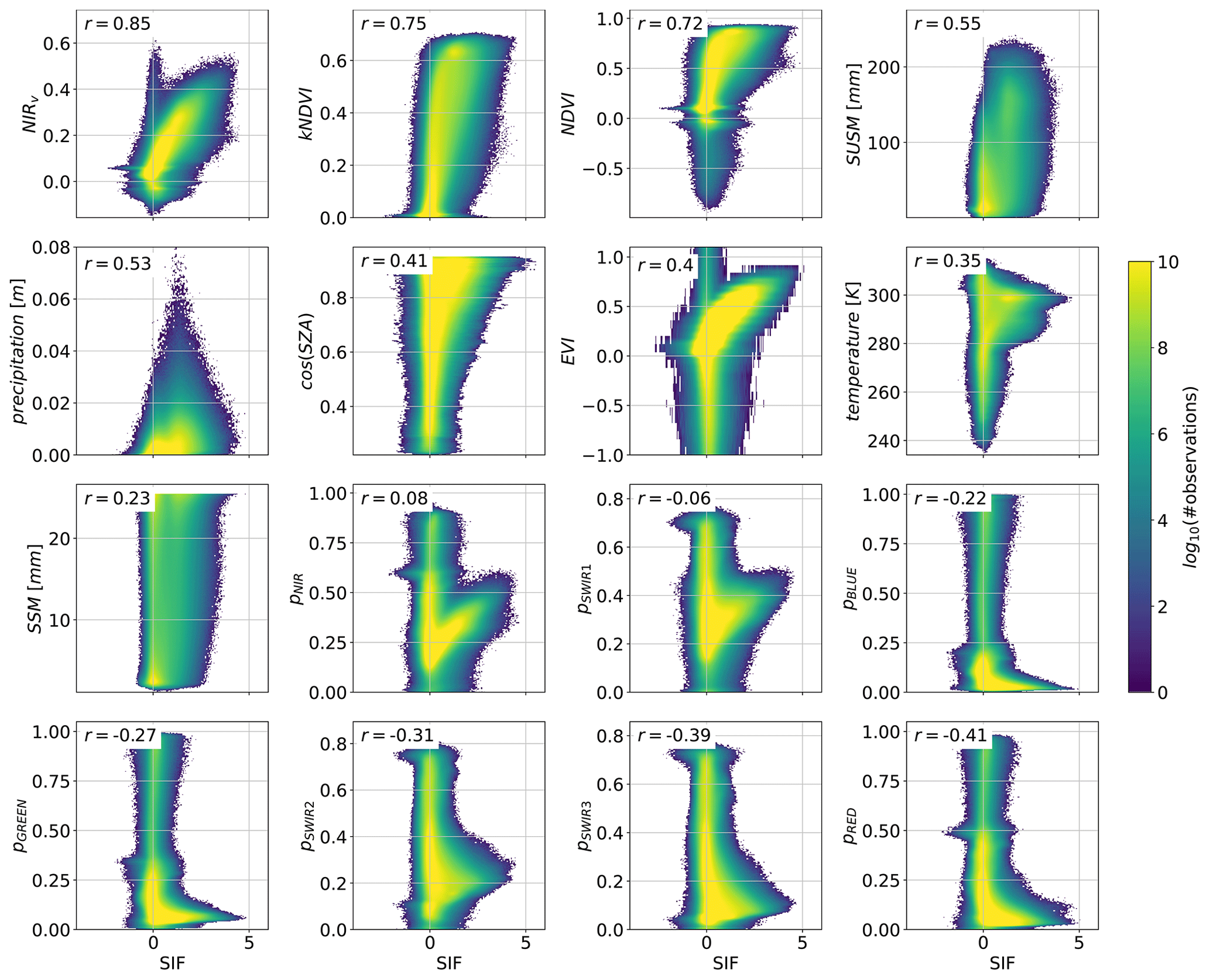
Figure 1Scatter comparison of SIF to timely changing auxiliary data. The time span of measurements is from April 2018 to March 2021 at 16 d resolution. Longitude and latitude borders are from −180 to 180∘ and −60 to 70∘, respectively. The comparison resolution corresponds to the lowest resolution of the two corresponding products. For all MODIS data the resolution is 0.05∘ and for precipitation, air temperature, surface soil moisture (ssm), and subsurface soil moisture (susm) 0.1∘. To quantify the goodness of fit we compute the Pearson correlation coefficient (r) for each subplot (Benesty et al., 2009).
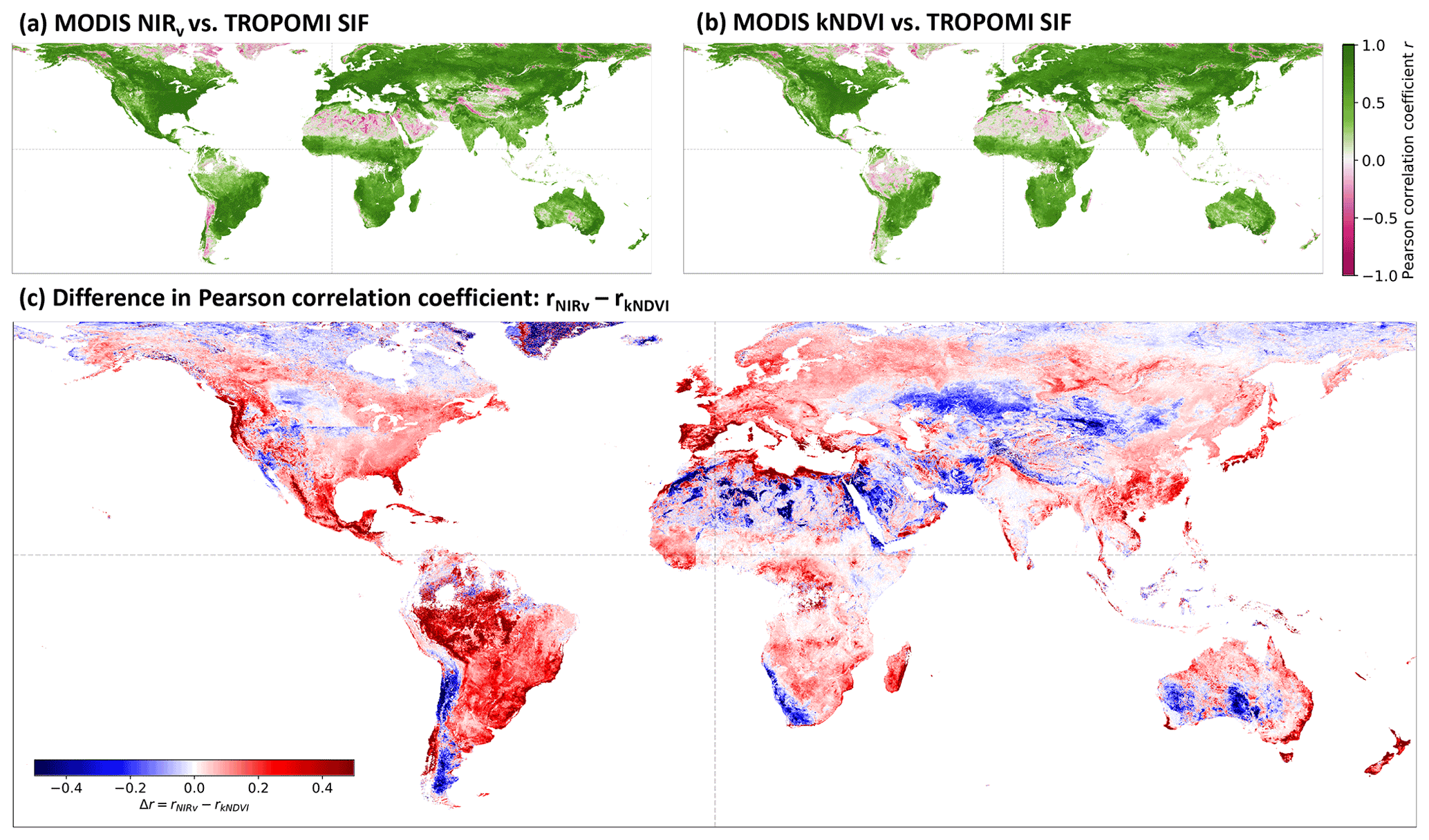
Figure 2Pearson correlation coefficient of NIRv and kNDVI to TROPOMI SIF. Data are compared at 0.05∘ spatial resolution and in 16 d time steps starting in April 2018 until March 2021. The value per grid cell in (a) and (b) represents the Pearson correlation coefficient of the vegetation index to SIF in time. Panel (c) represents the difference in correlation of the vegetation indices to SIF.
Figure 2 shows spatial patterns of the Pearson correlation coefficients between both NIRv and kNDVI to SIF. In both our spatial (Fig. 2) and temporal (Fig. 1) analyses, we find NIRv is a better predictor for SIF than kNDVI, which contradicts the recent findings from Camps-Valls et al. (2021). However, Camps-Valls et al. (2021) used GOME-2 SIF instead of TROPOMI SIF.
The vegetation index NIRv outperforms kNDVI in nearly all vegetated regions. Only central Asia, the Sahara, and very high latitudes show a better correlation of kNDVI with SIF. At the same time, these regions generally show a weaker correlation of vegetation indices with SIF.
3.1 Training and optimization of the neural network
Convolutional neural networks (CNNs) are supervised machine learning methods that need matching feature and ground truth data pairs to compute the loss that is back propagated (Bishop, 2007). As such, we begin by coarsening SIF data to 0.5∘ and use it with auxiliary data at 0.05∘ as input to SIFnet, allowing us to estimate SIF at 0.05∘. The model output is compared against the measured TROPOMI SIF at 0.05∘. After optimizing the model it can resolve a scaling factor of 10 between coarse-resolution input SIF and model output SIF. Figure 3 visualizes this method. In the following step of estimating high-resolution SIF, the feature SIF data have a resolution of 0.05∘ and auxiliary data of 0.005∘, resulting in a model output of SIF at 0.005∘.

Figure 3CNN model structure and training and estimation method. Yellow and red blocks are convolutional and ReLU layers, respectively. Notation of convolutional layers: k(X1,X2): kernel sizes are X1,X2; chY: number of channels is Y. For training, the data are upscaled. We input auxiliary data at the target resolution and SIF data at a factor of 10 coarser.
Figure 3 shows our chosen CNN model structure for SIFnet. The model consists of convolutional and rectified linear unit (ReLU) layers that are arranged in a sequence. After the first convolutional block there is a residual connection that skips one ReLU and two convolutional layers. Convolutional kernel sizes are either (3,3) or (1,1). This structure is adapted from the literature findings from, for example, Lim et al. (2017). Further, several model structures (Sect. S4.3 in the Supplement) with a different amount of layers, channels, or residual blocks are compared. The chosen model structure represents the best trade-off between complexity and performance. The input feature collinearity and principal component analysis (PCA) presented in Sect. S3 show that some input features have high correlations with each other. A total of 9 out of the 19 PCs in the time variant and 13 out of the 15 PCs in the time-invariant data carry above 99 % of the variance. This suggests that fewer channels should be used in the CNN layers than the feature dimension (because some variables are similar). Therefore the number of channels in the first layer of SIFnet reduces the complexity from 34 to 16 channels (Fig. 3). More complex model structures did not result in a notably improved loss metrics (Sect. S4.3).
For training SIFnet we use 3 years of data (April 2018–March 2021) in 16 d time steps. The study regions are shown in Sect. S2. There are five folds used as training data: two folds over Asia, one over Europe, one over the southern part of Africa, and one over South America. Our validation region is North America (Fig. S4). The hyperparameter tuning is done by training the model on the five folds and computing the loss of the validation data. The parameters are optimized to minimize the loss of the validation data set. Due to computational reasons and the size of the data set, we do not apply a cross validation in the optimization process. The final product consists of high-resolution SIF at 0.005∘ and is validated against independent SIF measurements of the instruments OCO-2 and OCO-3.
We center and scale each feature individually by subtracting the mean and normalizing by the standard deviation. For data augmentation of the training data, we use random crops and random flips. Each day of one fold has a matrix size of 1200 × 900 pixels. We analyze 69 d in 16 d steps over 3 years. For each input during the training process we randomly crop a matrix with a size of 100 × 100 pixels. As some areas have a large fraction of missing values (e.g., due to water or clouds), we only use cropped matrices that consist of > 80 % valid pixels in the SIF product. Further, we randomly flip vertically and horizontally, both with a probability of 0.5. These data augmentation methods provide us with a huge database that should avoid overfitting the network parameters. During training, all missing values in the data are set to zero. That mainly affects water regions as the share of missing values in the SIF data used is 91.2 % caused by water. In case there is a missing value in the SIF training sample, all feature values of this pixel are also set to zero to ensure the network does not learn false relationships between the predictors and the target variable (that also applies to vegetated regions). For the MODIS bands we applied the quality index value 0 (best quality only). This filtering also removes pixels that include clouds. To ensure a high coverage we interpolated in time for MODIS. Further, training and test folds are selected based on coverage; i.e., the regions near the Equator (between ±22.5∘) are not included in the data cubes as MODIS reflectance is sensitive to clouds which appear frequently in these regions (compare Figs. S2 and S4). All static variables have full coverage on land. ERA5 data has full spatial and temporal coverage. We did not apply any further quality filtering on SMAP soil moisture data. The data are provided as a level 3 product on Google Earth Engine.
Our individual loss function is comprised of two loss terms. We use the mean squared error (MSE) loss in combination with the structural dissimilarity index (DSSIM). The DSSIM is the countermeasure of the structural similarity index (SSIM): DSSIM = 1 − SSIM (Brunet et al., 2011). Therefore, we are not only optimizing the overall deviation of the estimated SIF to the measured SIF but also the structural patterns. Section S4.4 shows the benefit of including both MSE and SSIM terms in the loss function. Equation (5) shows our loss function:
where n is the number of data points, yi is the data point i in measured (target variable) SIF, is the data point i in estimated SIF, Y values are all data points of measured (target variable) SIF, values are all data points of estimated SIF, μY is the mean of Y, is the mean of , σY is the variance of Y, is the variance of , is the covariance of Y and , and c1=(k1L)2 and c2=(k2L)2 are variables for stabilization with L= 2 bit px, k1=0.01, and k2=0.03. The parameters a and b define the weights of the overall loss of the two individual losses. The overall model performance did not show a notable sensitivity to different a and b values. To approximately keep the individual losses in the same order of magnitude, we set a=1 and b=0.3. DSSIM is in the range of 0 to 1, with 0 meaning structurally similar and 1 structurally dissimilar.
We use the optuna library for the hyperparameter tuning of the learning rate, weight decay, and epoch of the CNN (Akiba et al., 2019). Here, a tree-structured Parzen estimator sampler suggests the parameters of the next trial which is based on a Gaussian mixture model. Section S4.1 provides more details on this hyperparameter tuning.
3.2 Results of model optimization
Figure 4 summarizes the results of the optimized model. We observe an overall r2 of 0.92, SSIM of 0.87, and RMSE of 0.17 mW m−2 sr−1 nm−1 between the estimated SIF from SIFnet and retrieved SIF from TROPOMI at 0.05∘ (Fig. 4e). SSIM is calculated by comparing the average SIF signal of the 3 years under investigation. Figure 4e shows the three metrics for each month of the year. We observe the lowest r2 values in January, February, and March. These are associated with low SIF values and, consequently, lower signal-to-noise ratios which drive the decreased performance. SSIM also indicates reduced performance during this time period. RMSE values are correlated with overall productivity with the lowest RMSE in winter; this is expected as this metric depends on the magnitude of the signal.
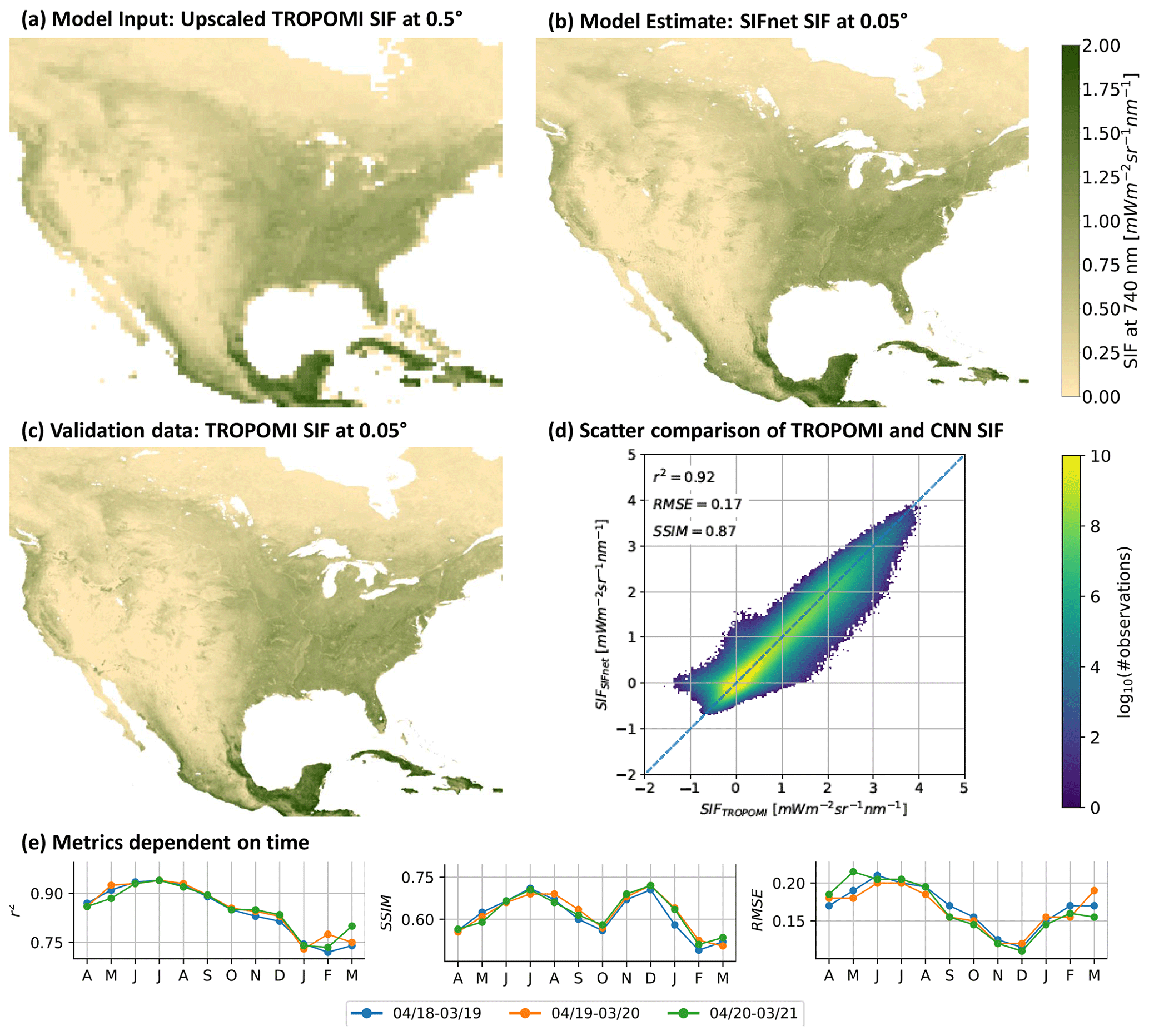
Figure 4Test set results of CNN training at 0.05∘. Panel (a) shows low-resolution SIF that is used as model input, (b) shows the estimated SIF at 0.05∘ by SIFnet, (c) shows the measured TROPOMI SIF at 0.05∘ from Köhler et al. (2018), (d) shows the scatter comparison between TROPOMI SIF and the SIFnet estimate at 0.05∘, and (e) shows for each investigated month the metrics r2, SSIM, and RMSE. Metrics are calculated at 16 d resolution and averaged to monthly values afterwards.
3.3 Which features drive SIFnet?
We are particularly interested in understanding which features drive our neural net. Here we evaluate the feature importance using the permutation feature importance method (Breiman, 2001; Fisher et al., 2019; Gregorutti et al., 2015, 2017) with our North American validation data at a target resolution of 0.05∘. The method first computes the RMSE including all input features (RMSEorig.). We then apply the following three steps.
-
Shuffle all pixels of one input feature randomly in time and space.
-
Compute the new RMSE of the estimation (RMSE).
-
Compare the shuffled RMSE to the original:
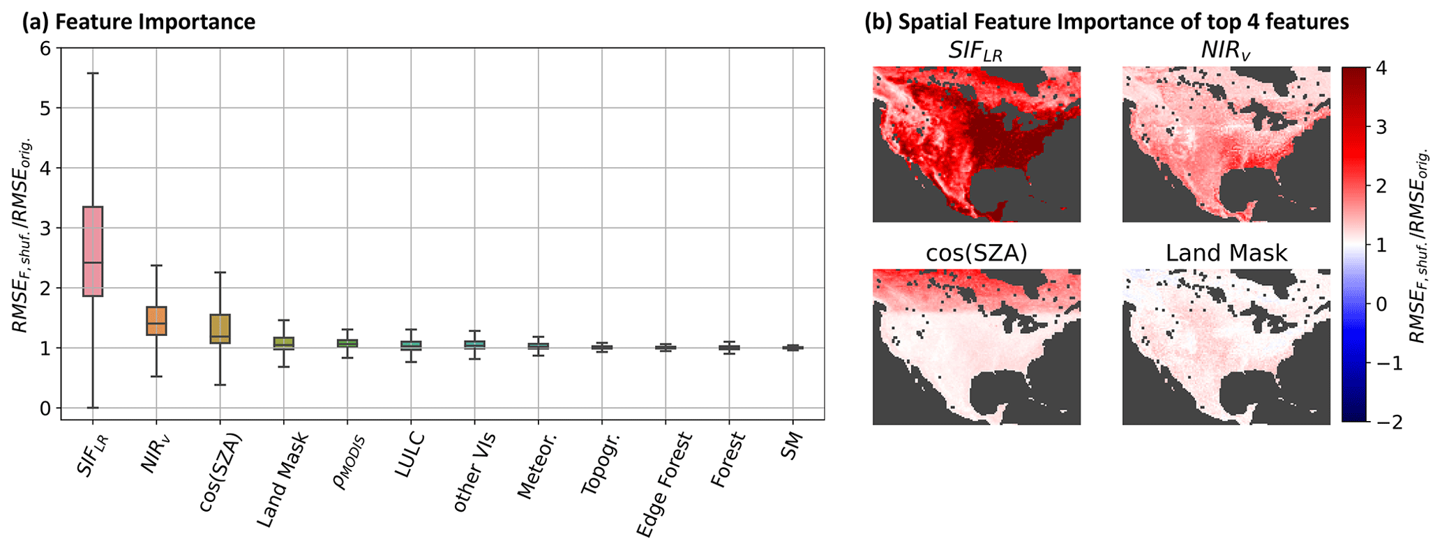
Figure 5Feature importance. Panel (a) shows the total RMSE of the permuted feature divided by the RMSE without feature permutation, and (b) shows the RMSE of each pixel with permuted features divided by the RMSE without feature permutation. Some input variables are clustered, and all variables of that class are permuted at the same time. ρMODIS: all seven MODIS bands; LULC: all 11 land cover classes; other VIs: kNDVI, NDVI, and EVI; Mereor.: temperature, precipitation, temperature with 16 d delay, and precipitation with 16 d delay; SM: surface soil moisture and subsurface soil moisture.
Figure 5 shows the feature importance of clustered input classes and individual features to the overall estimation. Multiple applications of the feature permutation yielded negligible differences in feature importance. Figure 5a shows the RMSE share of shuffled data to the RMSE of unshuffled data. SIFnet finds low-resolution SIF (SIFLR) to be the most important input variable, followed by the vegetation index NIRv and the cosine of the solar zenith angle (cos (SZA)). All other variables do not contribute notably to the model output. This result strengthens our findings from Figs. 1 and 2 that NIRv is better correlated with SIF from TROPOMI than kNDVI. Further, our feature importance is in line with Dechant et al. (2022) in which they find a high correlation of SIF with NIRv multiplied with photosynthetic active radiation (PAR), of which the cos (SZA) can be used as a proxy. The CNN is a data-driven method and is not restricted by LUE terms. Although SM and meteorology (air temperature and precipitation) play a key role for photosynthesis, we find that they are not important to our model output. This does not necessarily imply that SIF is not linked to these parameters. This can be explained by the following. (1) The variables SM and those from ERA-5 are at coarser resolution than the actual model output of the training phase which is at 0.05∘ (10 000 and 11 132 m for SM and ERA-5, respectively). Therefore each pixel at the resolution of 0.05∘ does not have its unique value for SM or ERA-5, but multiple cells can be within one SM or ERA-5 pixel. (2) Not only do the auxiliary data of the model estimate higher-resolution SIF, but they are computed together with coarse-resolution SIF. Therefore, events like heat stress that impact a bigger area than the actual model output might be represented in the coarse-resolution SIF. (3) We have aggregated the data used to 16 d time steps. LUE parameters influencing SIF might have a bigger impact on the estimation at higher temporal resolutions.
Figure 5b shows the spatial feature importance over the validation set in North America for the four most important features. We observe that SIFLR has the biggest impact in the eastern US, which corresponds strongly to the high vs. low productivity regions in the US. NIRv is a strong predictor in the southeastern US and in shrub regions in the western US. The contribution of cos (SZA) is highest at high latitudes and weakens at lower latitudes. NIRv is found to be less predictive of SIF at high latitudes. The land mask is the fourth most important input feature and contributes most in shrub regions. These four features consistently stand out as the strongest predictors. Other inputs such as fragmentation and soil moisture were not found to be strong predictors here. In Sect. S4.6 we test higher scaling factors between low- and high-resolution SIF. Even with scaling factors of 20 and 50 low-resolution SIF stays the most and second most important input feature, respectively.
We also examined different combinations of inputs such as directly including the MODIS bands as opposed to vegetation indices derived from MODIS bands (see Fig. S11). Low-resolution SIF remains the most important feature, followed by the NIR band ρNIR. The land cover products increase in relevance. Interestingly, when low-resolution SIF is omitted as input for the model, we observe contrasting results to Fig. 5 in which NIRv is no longer a leading predictor. We find that cos (SZA), ρNIR, kNDVI, and NDVI are the four most important features in this case (see Fig. S12). This may result from the collinearity between input features or suggests that another combination of ρNIR and ρRED is better correlated to SIF than, for example, NIRv or kNDVI. This finding was robust to multiple optimizations and permutations.
3.4 Comparison of SIFnet to downscaled SIF
Figure 6 shows the 0.005∘ SIF estimated by SIFnet and downscaled SIF from Turner et al. (2020). The difference between the two SIF estimates can be seen in Fig. 6c. SIFnet predicts lower SIF in the western US drylands and higher SIF over forested regions in the eastern US. This prediction of lower SIF in drylands is interesting because Turner et al. (2020) resorted to an ad hoc bias correction in these regions due to a low signal-to-noise ratio. Recent work from Wang et al. (2022) concluded that SIF and NIRv capture complementary events in western US drylands as a proxy for GPP and that the linear correlation of SIF to GPP was substantially lower in these regions compared to other vegetation types. We also observe systematic differences in the predicted SIF in urban areas. These regions are further evaluated in Fig. S17. Notably, the SIFnet estimate is systematically lower than the downscaling estimate in most urban regions examined here, Seattle being a notable exception. Both SIFnet and the downscaling approach allocate SIF to large urban parks and green spaces, but SIFnet predicts little-to-no SIF over the rest of the urban area. In particular, SIFnet estimates nearly zero SIF in the urban core of Los Angeles and San Francisco. SIFnet and the downscaling method predict comparable SIF as we move away from the urban core. Fine-scale features in the urban region are visible in both SIF estimates such as the Schiller Woods in Chicago (42.0∘ N, 87.8∘ W).
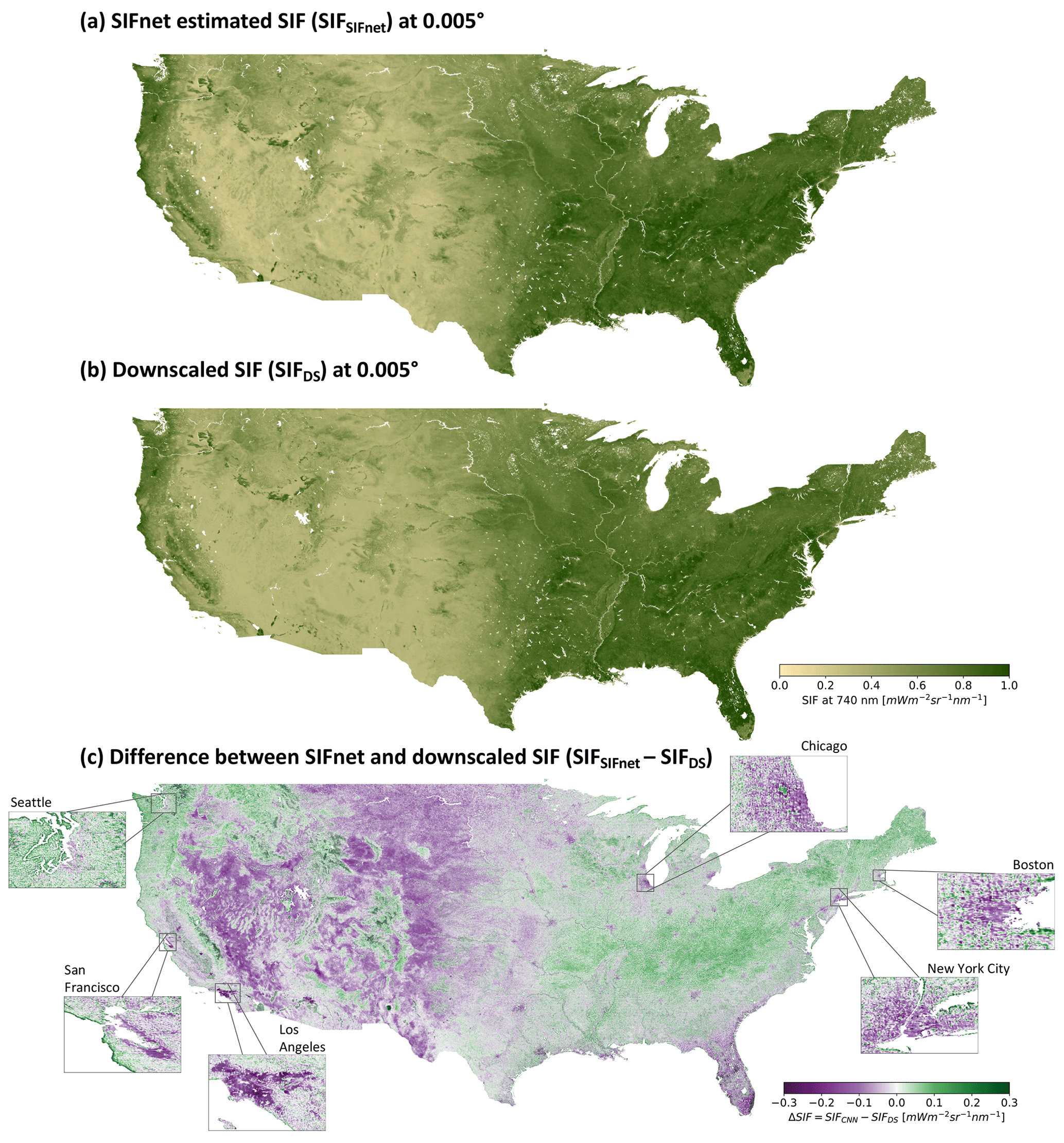
Figure 6SIFnet estimated SIF at 0.005∘ for CONUS and its comparison to downscaled SIF. Panel (a) shows the SIFnet estimated SIF at 0.005∘, (b) shows the downscaled SIF from Turner et al. (2020), and (c) shows the difference between SIFnet and downscaled SIF. Negative values imply a higher SIFnet SIF and positive values a higher downscaled SIF value.
The differences in SIF predicted from SIFnet and the downscaled SIF beg the question: which is correct? Here we evaluate both SIF products against independent SIF observations from OCO-2 and OCO-3 (OCO-2 Science Team/Michael Gunson, 2020; OCO-3 Science Team/Michael Gunson, 2020). These instruments have higher spatial resolution than TROPOMI and, as such, can be used to evaluate the high-resolution patterns predicted by both SIFnet and the downscaling approach. Specifically, OCO-2 and OCO-3 have nadir footprint sizes of 2.25 × 1.29 km. However, OCO-2 and OCO-3 do not provide full spatial coverage. They observe narrow swaths that are ∼ 10 km across-track. OCO-3 also provides a scanning mode to observe urban areas. Here, we use quality-checked OCO-2 data from April 2018 until March 2021 and OCO-3 data from July 2019 until March 2021. To compare the ungridded OCO-2 and OCO-3 data against the SIF estimated from TROPOMI, we compute the weighted average of all 0.005∘ grid cells that fall within the bounds of an OCO footprint. Here, the TROPOMI estimates are subsampled to 0.0005∘ (approx. 50 m at Equator), and the mean value is computed for all values which fall into the OCO footprint. For a quantitative comparison between OCO-2/3 and the SIFnet and downscaled estimate, the metrics r, r2, and RMSE are computed.
The high-resolution SIF estimates from SIFnet, the downscaling, and OCO are instantaneous SIF measurements taken at a specific time of the day, while the time of TROPOMI observations can differ substantially. Here, we compute the daily average SIF by scaling with the cosine of the SZA (Frankenberg et al., 2011):
where Daily SIF(x,y) is the daily integrated SIF estimate, is the instantaneous SIF at the individual measurement time, SZA is the solar zenith angle, τs is the time of the satellite measurement, τo is the time of sunrise, and τf is the time of sunset. This implicitly assumes that both PAR and SIF scale with cos (SZA) under cloud-free conditions, and we neglect Rayleigh scattering, as well as gas absorption. Although this approach neglects several water or light conditions, it provides our best estimate of daily SIF and enables comparison between multiple SIF products with different measurement times (Turner et al., 2021; Köhler et al., 2018; Frankenberg et al., 2011). The method is equivalent to the daily correction scheme for OCO-2, OCO-3, and TROPOMI (OCO-2 Science Team/Michael Gunson, 2020; OCO-3 Science Team/Michael Gunson, 2020; Frankenberg et al., 2011). Additionally, we performed a sensitivity study in which we trained SIFnet using daily corrected SIF and found the results to be generally insensitive to the use of instantaneous vs. daily corrected SIF (see Fig. S18). Following this, we chose to apply the daily correction after deriving the high-resolution SIF.
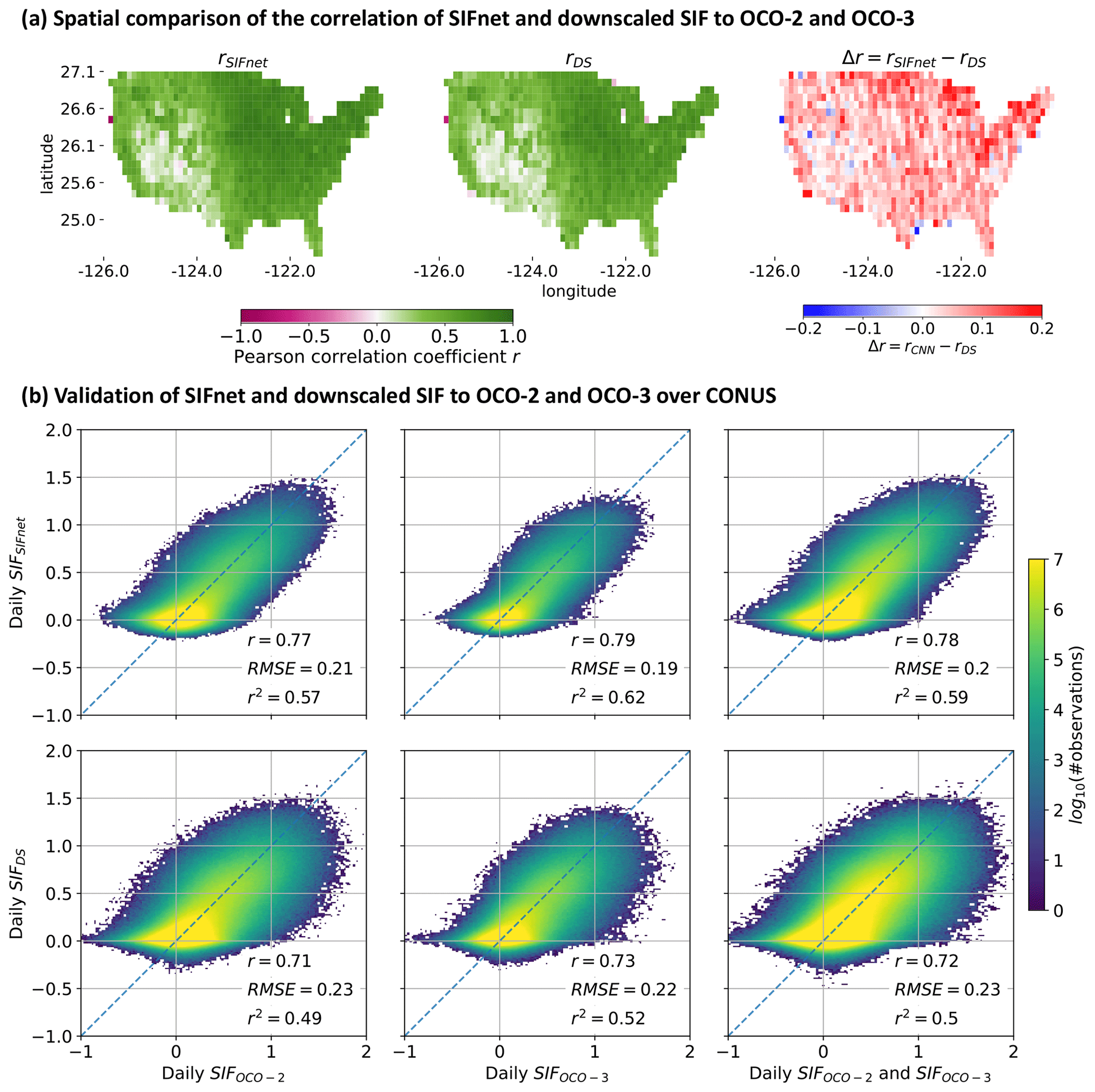
Figure 7Validation of SIFnet and downscaled SIF to OCO-2 and OCO-3 SIF over CONUS. Comparison from April 2018 until March 2021 in 16 d time steps. Daily OCO-2 and OCO-3 data are assigned to the closest 16 d time step. Panel (a) shows the gridded correlation of the two products against the combined data of OCO-2 and OCO-3. We first compute the SIF data from SIFnet and downscaling estimate that falls into the OCO footprint. Then we assign every OCO footprint to the closest grid point on the 1∘ grid dependent on the center location of that footprint and compute the Pearson correlation coefficient. Panel (b) shows the scatter comparison of the weighted average of all grid cells on the 0.005∘ estimated SIFnet SIF (ours) and downscaled SIF (Turner et al., 2020) that fall into the OCO-2 or OCO-3 footprint.
Figure 7 shows a comparison of both SIFnet and the downscaled SIF to OCO-2 and OCO-3. Specifically, Fig. 7a shows the correlation of SIFnet and the downscaled estimate with OCO-2/3 for every 1∘ pixel over CONUS. Both SIFnet and the downscaled SIF generally show good agreement with r in excess of 0.7 for most of the high-productivity regions. We observe weaker correlations in the western drylands due, in part, to a lower signal-to-noise ratio. Overall, we find SIFnet to perform systematically better than the downscaled SIF, as shown in the difference plot. Figure 7b summarizes these spatial patterns in a scatterplot comparison. SIFnet again shows better performance than the downscaled SIF against OCO-2, OCO-3, and OCO-2/3. The Pearson correlation coefficient r is 0.78 and 0.72 for the SIFnet and downscaled estimate, respectively, when comparing to all OCO data (right column in Fig. 7b). The generally high RMSE indicates different scales and variability in the data sets.
Deviations between TROPOMI and OCO-2/3 also appear at a grid of 0.05∘ (Fig. S19). The r2 coefficient is 0.61 and 0.62 between TROPOMI and OCO-2 and OCO-3 SIF, respectively. Indeed, one might expect better correlations here as both present SIF at 740 nm. However, as pointed out in Köhler et al. (2018), the uncertainty of both TROPOMI and OCO-2 SIF is expected to lead to a certain spread between the data sets. In addition, we do not account for differences in acquisition times and viewing–illumination geometry, which can lead to additional uncertainties in this comparison. For reference, when comparing single footprints of TROPOMI SIF to aggregated OCO-2 SIF for June 2018 globally, Köhler et al. (2018) found a r2 of 0.67; only additional aggregation leads to a r2 of 0.88. The mean deviation of TROPOMI SIF to OCO-2 SIF is close to the average standard deviation of TROPOMI SIF (0.4 mW m−2 sr−1 nm−1). In our analysis, from the 16 d product from TROPOMI SIF for April 2018 until March 2021 at 0.05∘, we observe an average error in the TROPOMI SIF of 0.43 mW m−2 sr−1 nm−1 for the CONUS. That error is close to the RMSE between instantaneous TROPOMI SIF and instantaneous OCO-2 SIF (0.37 mW m−2 sr−1 nm−1). To compare TROPOMI and OCO-2/3 SIF we aggregate the OCO-2/3 footprints to the same grid as our TROPOMI data (0.05∘). As we aggregate multiple OCO-2 or OCO-3 footprints to match one TROPOMI grid cell at 0.05∘, the certainty of the OCO measurements increases, and therefore the RMSE between TROPOMI and OCO SIF decreases.
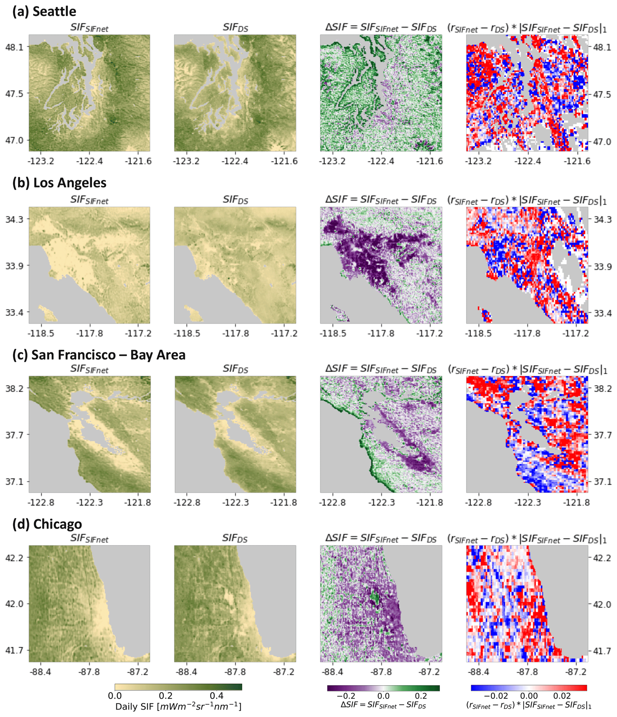
Figure 8SIFnet and downscaled SIF, the difference between these, and the difference in correlation to OCO-2 and OCO-3 for four urban regions. The first column shows the SIFnet estimate, the second the downscaled SIF from Turner et al. (2020), the third the difference between SIFnet and downscaled SIF, and the last the difference in correlation of the high-resolution SIF estimates to combined OCO-2 and OCO-3 data on a 0.02∘ grid multiplied with the ℒ1 norm between the SIFnet and downscaled estimate.
Figure 8 presents a detailed comparison of SIFnet and the downscaled SIF in four US cities. The first column shows the SIFnet estimate, the second the downscaled SIF from Turner et al. (2020), the third the difference between SIFnet and downscaled SIF, and the last column the difference in correlation of the high-resolution SIF estimates to combined OCO-2 and OCO-3 data on a 0.02∘ grid multiplied by the ℒ1 norm between the SIFnet and the downscaled SIF. The column on the right highlights both regions where the differences in predicted SIF are large and which product is performing better. As such, the right column will show white in areas where the difference in predicted SIF is small or the correlation with OCO is similar. While we observe large differences in predicted SIF for the urban areas (column 3), we do not find one product to perform systematically better in urban areas. This likely indicates the complexity in the SIF signal arising from urban areas. Additionally, urban areas make up a small fraction of the overall land mass and, as such, do not represent a large share of the training data in SIFnet. These factors likely contribute to the heterogeneous performance observed in the right column of Fig. 8.

Figure 9SIFnet SIF, downscaled SIF, MODIS NIRv, and a Google Earth cut-out for a part of Chicago. Left panel shows the SIFnet estimate, second panel shows the downscaled estimate from Turner et al. (2020), third panel shows MODIS NIRv for Chicago, and last panel shows the Google Earth cut-out (Google LLC, 2021). For panels 1–3 the average data for April 2018 until March 2021 is shown.
However, there are some notable successes of SIFnet in urban areas that can be mapped directly to features in the urban area. Figure 9 shows both SIFnet and the downscaled SIF along with NIRv from MODIS and a true color image of Chicago. A feature clearly stands out in both the downscaled SIF and NIRv image. This is a region with missing NIRv and effectively no downscaled SIF. However, SIFnet does not show a strong gradient here. This region corresponds to the Chicago airport. In the MODIS NIRv image it is visible that there are no valid data available for that region for the 3 investigated years. The downscaling method from Turner et al. (2020) relies only on NIRv in the weighting function. If there are no data available for the region, they are interpolated in space and time. Here, it shows that the method seems to fail in urban regions where no MODIS NIRv signal is available. SIFnet handles this region better and seems to rely on other auxiliary data if there is no MODIS NIRv available. In Fig. 8 it is also visible that the SIFnet estimate correlates better with the OCO-X data than the downscaled SIF for the region of the Chicago airport.
Here, we develop a convolutional neural network (CNN) model named SIFnet to increase the resolution of TROPOMI SIF by a factor of 10. The novelty of our method consists of using coarse-resolution SIF measurements together with high-resolution auxiliary data as model input to estimate high-resolution SIF. After optimization and hyperparameter tuning of SIFnet, the estimated SIF at 500 m resolution yields an r2 and RMSE of 0.92 and 0.17, respectively, when compared against validation data (Fig. 4). We further compare the output of SIFnet against a recently developed downscaling method to estimate high-resolution SIF (Turner et al., 2020) and evaluate both methods against independent observations from the Orbiting Carbon Observatory 2 and 3 (OCO-2/3). SIFnet is found to perform systematically better than the downscaling approach when compared against independent measurements. Through interpretable machine learning methods, we identify the key features that SIFnet utilizes to accurately predict high-resolution spatial patterns of SIF. We find that SIFnet relies heavily on the low-resolution SIF feature (SIFLR) and the vegetation index NIRv (Fig. 5).
SIFnet is a multi-layer CNN that increases the spatial resolution of the TROPOMI SIF by a factor of 10. Our model uses auxiliary data sets related to gross primary productivity and SIF as inputs and yields a high-resolution SIF estimate. The model is trained using three years of data from Asia, Europe, Africa, and South America. North America is used as the validation data set. Our loss function is comprised of two terms: the mean squared error and the structural dissimilarity index. The combination of these two terms improved the performance of our model.
SIFnet was further compared to the recent downscaled SIF product developed by Turner et al. (2020). The two high-resolution estimates showed pronounced differences across the western US drylands. This difference is particularly interesting because these drylands tend to be low-productivity regions and traditionally have been difficult for SIF to accurately capture due to the low signal-to-noise ratio. Both high-resolution SIF estimates were compared to independent observations from OCO-2/3. SIFnet performed systematically better than the downscaled SIF (r=0.78 for SIFnet, r=0.72 for downscaling). SIFnet and the downscaling method also yielded differences in urban regions. However, there was substantial heterogeneity in the performance of SIFnet and downscaling in urban areas. One product did not perform systematically better than the other within urban areas. The mixed results in urban areas likely relates to both the complexity of the photosynthetic activity in urban areas, as well as the lack of training data, as urban areas represent a small fraction of the total landmass.
We adapted techniques from the area of interpretable machine learning to assess the key features driving SIFnet. Specifically, we conducted random permutations to input data sets and assessed the impact on the resulting RMSE. From this, we found that SIFnet relies most heavily on the low-resolution SIF feature (SIFLR). The second most important factor is the MODIS vegetation index NIRv. NIRv is also found to outperform the recently proposed kNDVI vegetation index, in contrast to Camps-Valls et al. (2021). The interpretable machine learning approach also allowed us to identify spatial regions of importance for the different parameters. Interestingly, SIFnet relies more heavily on NIRv in the western drylands where the SIF signal-to-noise ratio is low. This implies that SIFnet is picking up on key physics that lead to the improved performance relative to the downscaling method. Overall, SIFnet represents a robust method to infer continuous high-spatial-resolution information about processes related to gross primary productivity.
The high-resolution SIF for CONUS from April 2018 until March 2021 is available here: https://doi.org/10.5281/zenodo.6321987 (Gensheimer et al., 2022). Further data can be requested from the authors.
The supplement related to this article is available online at: https://doi.org/10.5194/bg-19-1777-2022-supplement.
JG, AJT, and JC conceived the study. JG compiled data sets, conducted data analysis, and generated figures. JG wrote the manuscript. All authors edited the manuscript and provided feedback. JG did the literature research. PK and CF generated the TROPOMI SIF data. JC provided project guidance. All authors contributed to the discussion and interpretation of the results. All authors have read and agreed to the published version of the manuscript.
The contact author has declared that neither they nor their co-authors have any competing interests.
Publisher’s note: Copernicus Publications remains neutral with regard to jurisdictional claims in published maps and institutional affiliations.
We thank Xiaojing Tang, Luca Lloyd, and Lucy Hutyra from Boston University, USA, for providing us with their valuable global data about forest fragmentation.
This research has been supported by the Institute for Advanced Study, Technische Universität München (grant no. 291763), the Deutsche Forschungsgemeinschaft (grant no. 419317138), the NASA Early Career Faculty program (grant no. 80NSSC21K1808), and the NASA Carbon Cycle Science program (grant no. 80HQTR21T0101).
This work was supported by the German Research Foundation (DFG) and the Technical University of Munich (TUM) in the framework of the Open Access Publishing Program.
This paper was edited by Martin De Kauwe and reviewed by two anonymous referees.
Akiba, T., Sano, S., Yanase, T., Ohta, T., and Koyama, M.: Optuna: A next-generation hyperparameter optimization framework, in: KDD '19: Proceedings of the 25th ACM SIGKDD International Conference on Knowledge Discovery & Data Mining, 4–8 August 2019, Anchorage, AK, USA, 2623–2631, https://doi.org/10.1145/3292500.3330701, 2019. a
Badgley, G., Field, C. B., and Berry, J. A.: Canopy near-infrared reflectance and terrestrial photosynthesis, Science Advances, 3, e1602244, https://doi.org/10.1126/sciadv.1602244, 2017. a
Benesty, J., Chen, J., Huang, Y., and Cohen, I.: Pearson correlation coefficient, in: Noise reduction in speech processing, 37–40, Springer, ISBN 978-3-642-00295-3, 2009. a, b
Bishop, C. M.: Pattern Recognition and Machine Learning, Springer, 1st edn., New York, NY, ISBN 978-0-387-31073-2, 2007. a
Breiman, L.: Random forests, Mach. Learn., 45, 5–32, 2001. a
Brunet, D., Vrscay, E. R., and Wang, Z.: On the mathematical properties of the structural similarity index, IEEE T. Image Process., 21, 1488–1499, 2011. a
Buchhorn, M., Smets, B., Bertels, L., Roo, B. D., Lesiv, M., Tsendbazar, N.-E., Herold, M., and Fritz, S.: Copernicus Global Land Service: Land Cover 100 m: collection 3: epoch 2018: Globe, Zenodo [data set], https://doi.org/10.5281/zenodo.3518038, 2020. a, b
Camps-Valls, G., Campos-Taberner, M., Moreno-Martínez, Á., Walther, S., Duveiller, G., Cescatti, A., Mahecha, M. D., Muñoz-Marí, J., García-Haro, F. J., Guanter, L., and Jung, M.: A unified vegetation index for quantifying the terrestrial biosphere, Science Advances, 7, eabc7447, https://doi.org/10.1126/sciadv.abc7447, 2021. a, b, c, d
Castro, A. O., Chen, J., Zang, C. S., Shekhar, A., Jimenez, J. C., Bhattacharjee, S., Kindu, M., Morales, V. H., and Rammig, A.: OCO-2 solar-induced chlorophyll fluorescence variability across ecoregions of the Amazon basin and the extreme drought effects of El Niño (2015–2016), Remote Sens., 12, 1202, https://doi.org/10.3390/rs12071202, 2020. a
Chen, S., Liu, L., He, X., Liu, Z., and Peng, D.: Upscaling from Instantaneous to Daily Fraction of Absorbed Photosynthetically Active Radiation (FAPAR) for Satellite Products, Remote Sens., 12, 2083, https://doi.org/10.3390/rs12132083, 2020. a
Copernicus Climate Change Service (C3S): ERA5: Fifth generation of ECMWF atmospheric reanalyses of the global climate, Copernicus Climate Change Service Climate Data Store (CDS), https://cds.climate.copernicus.eu/cdsapp#!/home (last access: 13 August 2021), 2017. a
Danielson, J. J. and Gesch, D. B.: Global multi-resolution terrain elevation data 2010 (GMTED2010): U.S. Geological Survey Open-File Report 2011–1073, 26 pp., https://pubs.usgs.gov/of/2011/1073/ (last access: 20 August 2021), 2011. a
Dechant, B., Ryu, Y., Badgley, G., Köhler, P., Rascher, U., Migliavacca, M., Zhang, Y., Tagliabue, G., Guan, K., Rossini, M., and Goulas, Y.: NIRVP: A robust structural proxy for sun-induced chlorophyll fluorescence and photosynthesis across scales, Remote Sens. Environ., 268, 112763, https://doi.org/10.1016/j.rse.2021.112763, 2022. a
Duveiller, G., Filipponi, F., Walther, S., Köhler, P., Frankenberg, C., Guanter, L., and Cescatti, A.: A spatially downscaled sun-induced fluorescence global product for enhanced monitoring of vegetation productivity, Earth Syst. Sci. Data, 12, 1101–1116, https://doi.org/10.5194/essd-12-1101-2020, 2020. a
Entekhabi, D., Njoku, E. G., O'Neill, P. E., Kellogg, K. H., Crow, W. T., Edelstein, W. N., Entin, J. K., Goodman, S. D., Jackson, T. J., Johnson, J., and Kimball, J.: The soil moisture active passive (SMAP) mission, P. IEEE, 98, 704–716, 2010. a, b
Fisher, A., Rudin, C., and Dominici, F.: All Models are Wrong, but Many are Useful: Learning a Variable's Importance by Studying an Entire Class of Prediction Models Simultaneously, J. Mach. Learn. Res., 20, 1–81, 2019. a
Frankenberg, C., Fisher, J. B., Worden, J., Badgley, G., Saatchi, S. S., Lee, J. E., Toon, G. C., Butz, A., Jung, M., Kuze, A., and Yokota, T.: New global observations of the terrestrial carbon cycle from GOSAT: Patterns of plant fluorescence with gross primary productivity, Geophys. Res. Lett., 38, L17706, https://doi.org/10.1029/2011GL048738, 2011. a, b, c, d
Friedlingstein, P., Jones, M. W., O'Sullivan, M., Andrew, R. M., Hauck, J., Peters, G. P., Peters, W., Pongratz, J., Sitch, S., Le Quéré, C., Bakker, D. C. E., Canadell, J. G., Ciais, P., Jackson, R. B., Anthoni, P., Barbero, L., Bastos, A., Bastrikov, V., Becker, M., Bopp, L., Buitenhuis, E., Chandra, N., Chevallier, F., Chini, L. P., Currie, K. I., Feely, R. A., Gehlen, M., Gilfillan, D., Gkritzalis, T., Goll, D. S., Gruber, N., Gutekunst, S., Harris, I., Haverd, V., Houghton, R. A., Hurtt, G., Ilyina, T., Jain, A. K., Joetzjer, E., Kaplan, J. O., Kato, E., Klein Goldewijk, K., Korsbakken, J. I., Landschützer, P., Lauvset, S. K., Lefèvre, N., Lenton, A., Lienert, S., Lombardozzi, D., Marland, G., McGuire, P. C., Melton, J. R., Metzl, N., Munro, D. R., Nabel, J. E. M. S., Nakaoka, S.-I., Neill, C., Omar, A. M., Ono, T., Peregon, A., Pierrot, D., Poulter, B., Rehder, G., Resplandy, L., Robertson, E., Rödenbeck, C., Séférian, R., Schwinger, J., Smith, N., Tans, P. P., Tian, H., Tilbrook, B., Tubiello, F. N., van der Werf, G. R., Wiltshire, A. J., and Zaehle, S.: Global Carbon Budget 2019, Earth Syst. Sci. Data, 11, 1783–1838, https://doi.org/10.5194/essd-11-1783-2019, 2019. a
Gensheimer, J., Turner, A. J., Köhler, P., Frankenberg, C., and Chen, J.: TROPOMI SIF high resolution data at 0.005∘ for CONUS as estimated by the convolutional neural network SIFnet (1.0), Zenodo [data set], https://doi.org/10.5281/zenodo.6321987, 2022. a
Gentine, P. and Alemohammad, S.: Reconstructed solar-induced fluorescence: A machine learning vegetation product based on MODIS surface reflectance to reproduce GOME-2 solar-induced fluorescence, Geophys. Res. Lett., 45, 3136–3146, 2018. a
Google LLC: Google earth. Chicago, USA, 41.895∘ N–42.061∘ N, 88.016∘ W–87.7856∘ W, http://earth.google.com, last access: 15 December 2021. a
Gregorutti, B., Michel, B., and Saint-Pierre, P.: Grouped variable importance with random forests and application to multiple functional data analysis, Comput. Stat. Data An., 90, 15–35, 2015. a
Gregorutti, B., Michel, B., and Saint-Pierre, P.: Correlation and variable importance in random forests, Stat. Comput., 27, 659–678, 2017. a
Haddad, N. M., Brudvig, L. A., Clobert, J., Davies, K. F., Gonzalez, A., Holt, R. D., Lovejoy, T. E., Sexton, J. O., Austin, M. P., Collins, C. D., and Cook, W. M.: Habitat fragmentation and its lasting impact on Earth’s ecosystems, Science Advances, 1, e1500052, https://doi.org/10.1126/sciadv.1500052, 2015. a, b
Hanes, J.: Biophysical applications of satellite remote sensing, Springer Science & Business Media, https://doi.org/10.1007/978-3-642-25047-7, 2013. a, b
Huete, A., Didan, K., Miura, T., Rodriguez, E. P., Gao, X., and Ferreira, L. G.: Overview of the radiometric and biophysical performance of the MODIS vegetation indices, Remote Sens. Environ., 83, 195–213, 2002. a, b
Huete, A. R., Didan, K., Shimabukuro, Y. E., Ratana, P., Saleska, S. R., Hutyra, L. R., Yang, W., Nemani, R. R., and Myneni, R.: Amazon rainforests green-up with sunlight in dry season, Geophys. Res. Lett., 33, L06405, https://doi.org/10.1029/2005GL025583, 2006. a
Humphrey, V., Berg, A., Ciais, P., Gentine, P., Jung, M., Reichstein, M., Seneviratne, S. I., and Frankenberg, C.: Soil moisture–atmosphere feedback dominates land carbon uptake variability, Nature, 592, 65–69, 2021. a
Joiner, J., Yoshida, Y., Vasilkov, A. P., Yoshida, Y., Corp, L. A., and Middleton, E. M.: First observations of global and seasonal terrestrial chlorophyll fluorescence from space, Biogeosciences, 8, 637–651, https://doi.org/10.5194/bg-8-637-2011, 2011. a
Joiner, J., Guanter, L., Lindstrot, R., Voigt, M., Vasilkov, A. P., Middleton, E. M., Huemmrich, K. F., Yoshida, Y., and Frankenberg, C.: Global monitoring of terrestrial chlorophyll fluorescence from moderate-spectral-resolution near-infrared satellite measurements: methodology, simulations, and application to GOME-2, Atmos. Meas. Tech., 6, 2803–2823, https://doi.org/10.5194/amt-6-2803-2013, 2013. a
Jung, M., Koirala, S., Weber, U., Ichii, K., Gans, F., Camps-Valls, G., Papale, D., Schwalm, C., Tramontana, G., and Reichstein, M.: The FLUXCOM ensemble of global land-atmosphere energy fluxes, Scientific Data, 6, 1–14, 2019. a, b, c
Köhler, P., Frankenberg, C., Magney, T. S., Guanter, L., Joiner, J., and Landgraf, J.: Global retrievals of solar-induced chlorophyll fluorescence with TROPOMI: First results and intersensor comparison to OCO-2, Geophys. Res. Lett., 45, 10–456, 2018. a, b, c, d, e, f, g, h
Li, X. and Xiao, J.: A global, 0.05-degree product of solar-induced chlorophyll fluorescence derived from OCO-2, MODIS, and reanalysis data, Remote Sens., 11, 517, https://doi.org/10.3390/rs11050517, 2019. a, b
Lim, B., Son, S., Kim, H., Nah, S., and Mu Lee, K.: Enhanced deep residual networks for single image super-resolution, in: Proceedings of the IEEE conference on computer vision and pattern recognition workshops, 136–144, arXiv [preprint], arXiv:1707.02921, 10 July 2017. a
Magney, T. S., Bowling, D. R., Logan, B. A., Grossmann, K., Stutz, J., Blanken, P. D., Burns, S. P., Cheng, R., Garcia, M. A., Köhler, P., and Lopez, S.: Mechanistic evidence for tracking the seasonality of photosynthesis with solar-induced fluorescence, P. Natl. Acad. Sci. USA, 116, 11640–11645, 2019. a
Magney, T. S., Barnes, M. L., and Yang, X.: On the covariation of chlorophyll fluorescence and photosynthesis across scales, Geophys. Res. Lett., 47, e2020GL091098, https://doi.org/10.1029/2020GL091098, 2020. a, b
Mahadevan, P., Wofsy, S. C., Matross, D. M., Xiao, X., Dunn, A. L., Lin, J. C., Gerbig, C., Munger, J. W., Chow, V. Y., and Gottlieb, E. W.: A satellite-based biosphere parameterization for net ecosystem CO2 exchange: Vegetation Photosynthesis and Respiration Model (VPRM), Global Biogeochem. Cy., 22, GB2005, https://doi.org/10.1029/2006GB002735, 2008. a
Miller, J. B., Lehman, S. J., Verhulst, K. R., Miller, C. E., Duren, R. M., Yadav, V., Newman, S., and Sloop, C. D.: Large and seasonally varying biospheric CO2 fluxes in the Los Angeles megacity revealed by atmospheric radiocarbon, P. Natl. Acad. Sci. USA, 117, 26681–26687, 2020. a
Morreale, L. L., Thompson, J. R., Tang, X., Reinmann, A., and Hutyra, L. R.: Elevated growth and biomass along temperate forest edges, Nat. Commun., 12, 7181, https://doi.org/10.1038/s41467-021-27373-7, 2021. a
OCO-2 Science Team/Michael Gunson, A. E.: OCO-2 Level 2 bias-corrected solar-induced fluorescence and other select fields from the IMAP-DOAS algorithm aggregated as daily files, in: Retrospective processing V10r, Goddard Earth Sciences Data and Information Services Center (GES DISC), https://doi.org/10.5067/XO2LBBNPO010, 2020. a, b, c, d
OCO-3 Science Team/Michael Gunson, A. E.: OCO-3 Level 2 bias-corrected solar-induced fluorescence and other select fields from the IMAP-DOAS algorithm aggregated as daily files, in: Retrospective processing VEarlyR, Goddard Earth Sciences Data and Information Services Center (GES DISC), https://disc.gsfc.nasa.gov/datacollection/OCO3_L2_Lite_SIF_EarlyR.html (last access: 20 August 2021), 2020. a, b, c, d
PySolar: Python library PySolar, PySolar, https://github.com/pingswept/pysolar, last access: 30 September 2021. a
Reichstein, M., Falge, E., Baldocchi, D., Papale, D., Aubinet, M., Berbigier, P., Bernhofer, C., Buchmann, N., Gilmanov, T., Granier, A., and Grünwald, T.: On the separation of net ecosystem exchange into assimilation and ecosystem respiration: review and improved algorithm, Glob. Change Biol., 11, 1424–1439, 2005. a
Reinmann, A. B. and Hutyra, L. R.: Edge effects enhance carbon uptake and its vulnerability to climate change in temperate broadleaf forests, P. Natl. Acad. Sci. USA, 114, 107–112, 2017. a
Schaaf, C. and Wang, Z.: MCD43A4 MODIS/Terra+Aqua BRDF/Albedo Nadir BRDF Adjusted Ref Daily L3 Global – 500 m V006, NASA EOSDIS Land Processes DAAC [data set], https://doi.org/10.5067/MODIS/MCD43A4.006, 2015. a
Sellers, P. J.: Canopy reflectance, photosynthesis and transpiration, Int. J. Remote Sens., 6, 1335–1372, 1985. a
Shekhar, A., Chen, J., Bhattacharjee, S., Buras, A., Castro, A. O., Zang, C. S., and Rammig, A.: Capturing the impact of the 2018 european drought and heat across different vegetation types using OCO-2 solar-induced fluorescence, Remote Sens., 12, 3249, https://doi.org/10.3390/rs12193249, 2020a. a
Shekhar, A., Chen, J., Paetzold, J. C., Dietrich, F., Zhao, X., Bhattacharjee, S., Ruisinger, V., and Wofsy, S. C.: Anthropogenic CO2 emissions assessment of Nile Delta using XCO2 and SIF data from OCO-2 satellite, Environ. Res. Lett., 15, 095010, https://doi.org/10.1088/1748-9326/ab9cfe, 2020b. a
Siegmann, B., Cendrero-Mateo, M. P., Cogliati, S., Damm, A., Gamon, J., Herrera, D., Jedmowski, C., Junker-Frohn, L.V., Kraska, T., Muller, O., and Rademske, P.: Downscaling of far-red solar-induced chlorophyll fluorescence of different crops from canopy to leaf level using a diurnal data set acquired by the airborne imaging spectrometer HyPlant, Remote Sens. Environ., 264, 112609, https://doi.org/10.1016/j.rse.2021.112609, 2021. a
Sims, D. A., Rahman, A. F., Cordova, V. D., El‐Masri, B. Z., Baldocchi, D. D., Flanagan, L. B., Goldstein, A. H., Hollinger, D. Y., Misson, L., Monson, R. K., and Oechel, W. C.: On the use of MODIS EVI to assess gross primary productivity of North American ecosystems, J. Geophys. Res.-Biogeo., 111, G04015, https://doi.org/10.1029/2006JG000162, 2006. a
Smith, I. A., Hutyra, L. R., Reinmann, A. B., Marrs, J. K., and Thompson, J. R.: Piecing together the fragments: elucidating edge effects on forest carbon dynamics, Front. Ecol. Environ., 16, 213–221, 2018. a
Tucker, C. J.: Red and photographic infrared linear combinations for monitoring vegetation, Remote Sens. Environ., 8, 127–150, 1979. a
Turner, A. J., Köhler, P., Magney, T. S., Frankenberg, C., Fung, I., and Cohen, R. C.: A double peak in the seasonality of California's photosynthesis as observed from space, Biogeosciences, 17, 405–422, https://doi.org/10.5194/bg-17-405-2020, 2020. a, b, c, d, e, f, g, h, i, j, k, l, m, n, o
Turner, A. J., Köhler, P., Magney, T. S., Frankenberg, C., Fung, I., and Cohen, R. C.: Extreme events driving year-to-year differences in gross primary productivity across the US, Biogeosciences, 18, 6579–6588, https://doi.org/10.5194/bg-18-6579-2021, 2021. a, b, c, d, e, f
Wang, X., Biederman, J. A., Knowles, J. F., Scott, R. L., Turner, A. J., Dannenberg, M. P., Köhler, P., Frankenberg, C., Litvak, M. E., Flerchinger, G. N., Law, B. E., Kwon, H., Reed, S. C., Parton, W. J., Barron-Gafford, G. A., and Smith, W. K.: Satellite solar-induced chlorophyll fluorescence and near-infrared reflectance capture complementary aspects of dryland vegetation productivity dynamics, Remote Sens. Environ., 270, 112858, https://doi.org/10.1016/j.rse.2021.112858, 2022. a
Wu, D., Lin, J. C., Duarte, H. F., Yadav, V., Parazoo, N. C., Oda, T., and Kort, E. A.: A model for urban biogenic CO2 fluxes: Solar-Induced Fluorescence for Modeling Urban biogenic Fluxes (SMUrF v1), Geosci. Model Dev., 14, 3633–3661, https://doi.org/10.5194/gmd-14-3633-2021, 2021. a
Yu, L., Wen, J., Chang, C., Frankenberg, C., and Sun, Y.: High-resolution global contiguous SIF of OCO-2, Geophys. Res. Lett., 46, 1449–1458, 2019. a
Zeng, J., Matsunaga, T., Tan, Z.-H., Saigusa, N., Shirai, T., Tang, Y., Peng, S., and Fukuda, Y.: Global terrestrial carbon fluxes of 1999–2019 estimated by upscaling eddy covariance data with a random forest, Scientific Data, 7, 1–11, 2020. a
Zhang, Y., Joiner, J., Alemohammad, S. H., Zhou, S., and Gentine, P.: A global spatially contiguous solar-induced fluorescence (CSIF) dataset using neural networks, Biogeosciences, 15, 5779–5800, https://doi.org/10.5194/bg-15-5779-2018, 2018. a
Zhang, Z., Xu, W., Qin, Q., and Long, Z.: Downscaling Solar-Induced Chlorophyll Fluorescence Based on Convolutional Neural Network Method to Monitor Agricultural Drought, IEEE T. Geosci. Remote, 59, 1012–1028, https://doi.org/10.1109/TGRS.2020.2999371, 2021. a