The onset of the spring phytoplankton bloom in the coastal North Sea supports the Disturbance Recovery Hypothesis

The spring phytoplankton bloom is a key event in temperate and polar seas, yet the mechanisms that trigger it remain under debate. Some hypotheses claim that the spring bloom onset occurs when light is no longer limiting, allowing phytoplankton division rates to surpass a critical threshold. In contrast, the Disturbance Recovery Hypothesis (DRH) proposes that the onset responds to an imbalance between phytoplankton growth and loss processes, allowing phytoplankton biomass to start accumulating, and this can occur even when light is still limiting. Although several studies have shown that the DRH can explain the spring bloom onset in oceanic waters, it is less certain whether and how it also applies to coastal areas. To address this question at a coastal location in the Scottish North Sea, we combined 21 years (1997–2017) of weekly in situ chlorophyll and environmental data with meteorological information. Additionally, we also analyzed phytoplankton cell counts estimated using microscopy (2000–2017) and flow cytometry (2015–2017). The onset of phytoplankton biomass accumulation occurred around the same date each year, 16 ± 11 d (mean ± SD) after the winter solstice, when light limitation for growth was strongest. Also, negative and positive biomass accumulation rates (r) occurred respectively before and after the winter solstice at similar light levels. The seasonal change from negative to positive r was mainly driven by the rate of change in light availability rather than light itself. Our results support the validity of the DRH for the studied coastal region and suggest its applicability to other coastal areas.

1 Introduction

The spring bloom is a major seasonal feature of temperate and polar seas and plays significant ecological and biogeochemical roles (Townsend et al., 1994). Although scientists generally agree that this event corresponds to an accumulation of large phytoplankton biomass, no consensus has been reached on how it is initiated, even after more than a century of research (Behrenfeld and Boss, 2014, 2018). Despite this ongoing discussion, all current theories attempt in essence to understand how phytoplankton biomass starts to accumulate; i.e., how the biomass accumulation rate (r), which is the difference between phytoplankton division and loss rates (μ and l, respectively), becomes positive. It is worth noting that the accumulation of phytoplankton biomass is not constant during the spring bloom and at short time scales, positive and negative r often alternate. Thus, the bloom initiation is actually the moment when r first becomes predominantly positive, eventually allowing phytoplankton to reach the seasonal biomass peak (Behrenfeld and Boss, 2018).

The more traditional school of thought assumes that the spring bloom is triggered when the winter light limitation relaxes to a point that allows μ to surpass a critical threshold (Behrenfeld and Boss, 2014, 2018). To this pure bottom-up view belong for instance the famous Critical Depth Hypothesis (Gran and Braarud, 1935; Sverdrup, 1953) and Critical Turbulence Hypothesis (Huisman et al., 1999). An alternative framework focuses on processes that lead to positive r by disrupting the equilibrium between phytoplankton division and loss processes, especially grazing and virus infections, and this disruption can occur even when light is still limiting. The importance of this equilibrium disruption for the spring bloom development has been addressed by several studies, such as Evans and Parslow (1985) and Banse (1994). More recently, this framework has been deeply reviewed and formalized in the Disturbance Recovery Hypothesis (DRH, Behrenfeld et al., 2013; Behrenfeld and Boss, 2014).

The DRH suggests, for instance, that positive r observations in early winter are possible if mixed layer deepening has a stronger negative impact on l, by reducing plankton encounter rates through dilution effects, than on μ, by increasing light limitation (Behrenfeld, 2010; Behrenfeld and Boss, 2018). Also, in opposition to the other school of thought, the DRH states that r follows the rate of change in division rates ($\mathrm{d}\mathit{\mu }/\mathrm{d}t$) rather than μ itself (Behrenfeld et al., 2013; Behrenfeld and Boss, 2018). According to this idea, an acceleration in μ impacts the μ–l balance, allowing phytoplankton to bloom (i.e., to accumulate biomass).

Although the DRH is supported by satellite and field observations in oceanic waters (Behrenfeld and Boss, 2018), we are not aware of any study showing how this hypothesis explains the spring bloom onset in coastal areas. Although these areas cover a small percentage of the ocean surface, they are among the most productive in the world (Mann, 2009) and provide important ecosystem services (Barbier, 2017). However, they are also under intense human pressure, as the global population is highly concentrated along the coastline (Cloern et al., 2016). Mignot et al. (2018) suggested that in coastal ecosystems, low variations in the mixed layer depth would decrease the importance of plankton dilution effects, probably leading to no phytoplankton biomass accumulation in winter. Nevertheless, according to the DRH, an early μ acceleration driven for example by a seasonal improvement in light conditions (i.e., by an accelerating increase in light availability) could still trigger a phytoplankton biomass accumulation in winter. This is plausible considering that coastal waters usually have high nutrient and turbidity levels during winter and spring (Mann, 2009), making light the main limiting factor for phytoplankton growth, especially at high latitudes with low surface light intensities and stormy weather.

To study how the spring phytoplankton bloom starts in the Scottish coastal North Sea, we combined 21 years (1997–2017) of weekly in situ chlorophyll and environmental data and meteorological information with phytoplankton cell counts estimated using microscopy (2000–2017) and flow cytometry (2015–2017). In particular, we addressed the questions: (1) does the spring bloom start in winter in the absence of a deepening in the mixed layer?, (2) is light availability a main driver of the process?, and (3) does the DRH hold true?

2 Material and methods

2.1 Monitoring site and environmental variables

The time series analyzed was collected at the Marine Scotland Scottish Coastal Observatory monitoring site at Stonehaven (56^∘57.8^′ N, 02^∘06.2^′ W, northwestern North Sea), a 48 m depth coastal station located 5 km offshore (Bresnan et al., 2009, 2015, 2016). This station has been sampled at a weekly frequency (weather permitting) since January 1997. In this study, data collected up to December 2017 were used (Marine Scotland Science, 2018). At a local scale, this coastal area is affected by strong tidal currents and winds, leading to a well-mixed water column for most of the year (Van Leeuwen et al., 2015; Bresnan et al., 2016). Although our study location is often taken to be representative of a larger hydrodynamic region (Van Leeuwen et al., 2015), the measured time series of phytoplankton and environmental variables are inevitably influenced by advective processes and no correction has been made for advection.

Different physicochemical variables were sampled to characterize the water column environment. Total Oxidized Nitrogen (TOxN) concentration, considered as a general proxy of nutrient concentration (Bresnan et al., 2009), and salinity were measured from water collected at surface and bottom depths (0–5 and ∼ 45 m, respectively) using Niskin bottles. Salinity was estimated using a Guildline 8410A Portasal salinometer and to measure TOxN concentrations, samples were stored at −20 ^∘C and thawed for 24 h before being analyzed by colorimetry using a continuous flow analysis system (Armstrong et al., 1967). The Niskin bottles were also equipped with digital reversing thermometers to record water temperature. Secchi disk depths (Z_SD) have been measured since 2001 to estimate light attenuation (K_d) of the water column. For this, we followed Devlin et al. (2008) and calculated relationships between Z_SD and K_d specific for the Stonehaven site (Sect. S1 and Fig. S1). Also, water was sampled using a 10 m Lund tube to obtain integrated surface chlorophyll a (Chl) concentrations and phytoplankton community information. For Chl analysis, depending on time of year, a subsample of 1 or 2 L (rarely 500 mL) was filtered through a GF/F filter and stored at −80 ^∘C until it was extracted in acetone and analyzed fluorometrically following the method of Arar and Collins (1992). Phytoplankton community counts since 2000 were performed using an inverted microscope at ×200 magnification (taxa with mean cell diameters generally >10 µm, Table S1 in the Supplement). For a full description of all sampling and laboratory procedures, see Bresnan et al. (2016). Lund tube water samples since 2015 were also analyzed using a BD Accuri™ C6 flow cytometer to estimate pico- and nanophytoplankton abundances, which rarely exceeded 10 µm cell diameter (for a full description of the flow cytometry methodology, see Tarran and Bruun, 2015).

As light is one of the main limiting factors for phytoplankton growth in coastal waters of the North Sea (Reid et al., 1990), we also estimated daily photosynthetic active radiation (PAR) at the sea surface and within the water column (Sects. S2–S3 and Figs. S2–S3). First, we estimated surface PAR (PAR_Sfc) using daily sunshine durations recorded at the Dyce meteorological station (57^∘12.3^′ N, 2^∘12.2^′ W, Met Office, 2012), located 27.6 km away from the Stonehaven site. Then, using K_d and PAR_Sfc estimations, we calculated average attenuated PAR (PAR_Att) for the top 10 m layer (where phytoplankton samples were collected) and for the entire water column (PAR_Att,10 and PAR_Att,48, respectively). Without vertical profiles of physical variables, we could not estimate the mixed layer depth, usually used as an estimation of the active turbulent layer (although this is often shallower, Franks, 2014). This turbulent layer determines how deep phytoplankton can be moved away from surface layers and, consequently, the amount of PAR they receive. Thus, we calculated PAR_Att,10 and PAR_Att,48 to estimate the range within the actual PAR experienced by phytoplankton. Both PAR_Sfc and PAR_Att are reported in µmol m⁻² s⁻¹.

2.2 Phytoplankton biomass accumulation rates (r) and spring bloom parameters

The analysis of the spring phytoplankton bloom requires estimating changes through time in biomass accumulation rates, r (Behrenfeld and Boss, 2018). We first transformed Chl into carbon (C) biomass of the entire phytoplankton community (C_phyto, mg C m⁻³) using an average seasonality of C : Chl ratios, estimated by combining microscopy and flow cytometry counts with cell data from the literature (Sects. S4–S5, Fig. S4 and Tables S1–S3).

Once C_phyto was estimated, we calculated r between two sampling dates separated by a period of time ($\mathrm{\Delta }t=t_{\mathrm{2}}-t_{\mathrm{1}}$) as:

$$\begin{array}{}\text{(1)}& r={\displaystyle \frac{\ln \left(C_{\mathrm{phyto},\mathrm{2}}\right)-\ln \left(C_{\mathrm{phyto},\mathrm{1}}\right)}{\mathrm{\Delta }t}}.\end{array}$$

To filter short-term variations in phytoplankton biomass and focus on the main winter–spring phenology pattern, we chose Δt to match the average e-folding timescale (T_e) of the spring bloom (Mignot et al., 2018), calculated as:

$$\begin{array}{}\text{(2)}& T_e={\displaystyle \frac{t_{max\mathrm{C}}-t_{min\mathrm{C}}}{\ln \left(C_{\mathrm{phyto}max}\right)-\ln \left(C_{\mathrm{phyto}min}\right)}},\end{array}$$

where t_min C and t_max C correspond respectively to the date when C_phyto was minimum and maximum between December and May (we considered t_max C as the timing of the spring bloom peak). The average T_e was 32.1 ± 9.0 d (mean ± SD) and thus, we selected t₂ to be the fourth sampling date after t₁ ($\mathrm{\Delta }t=\mathrm{31.4}\pm \mathrm{8.4}$ d). The possibility that using an average C : Chl seasonality artificially modified the general seasonal r pattern was discarded (Fig. S5).

We also calculated the spring bloom onset (t₀), defined as the first date after November when r was positive for at least 15 consecutive days, and the date when r was maximum between December and May (t_maxr). Before calculating t₀ and t_maxr, r was linearly interpolated between sampling dates to generate daily r estimates. To estimate environmental conditions at t₀ and t_maxr, we also linearly interpolated surface PAR, temperature and salinity, the difference between surface and bottom temperature and salinity, and the concentration of TOxN, Chl, and log-transformed C_phyto.

2.3 Statistical analysis

Seasonal mean environmental conditions were described using generalized additive models (GAMs) with a cyclic cubic regression spline (Wood, 2017) to identify potential factors driving the spring bloom onset. The visual inspection of these average seasonalities together with several exploratory analyses, such as GAMs including potential drivers of r at different time lags (not shown here), allowed discarding most of these drivers (see the Results and Discussion sections). Then, to test which type of hypothesis better explains the spring bloom onset, we correlated r with average daily PAR or average daily rate of change in PAR ($\mathrm{dPAR}/\mathrm{d}t$) for a period around the mean t₀. Daily PAR and $\mathrm{dPAR}/\mathrm{d}t$ were averaged from t₁ to t₂−1 d (see Eq. 1), as sampling generally occurred in the morning (09:30 ± 1.45 h GMT, mean ± SD). For these correlations, we excluded averages estimated with fewer than 15 PAR values.

All analyses and plots were performed in R v4.0.3 (R Core Team, 2020), using the Rstudio interface v1.3.1093 (Rstudio Team, 2020) and the tidyverse packages v1.3.0 (Wickham et al., 2019).

3 Results

3.1 Interannual variability and seasonality of the spring bloom

Phytoplankton biomass showed a clear seasonal pattern where the spring bloom was a major feature (Figs. 1 and 2). The analysis of bloom parameters revealed that although the spring bloom onset (t₀) had low interannual variability (6 January ± 11 d, mean ± SD), the timing of maximum r (t_max r, 9 April ± 18 d) and bloom peak (t_max C, 8 May ± 14 d) changed more from year to year. The maximum r and peak biomass showed the strongest interannual variability (0.070 ± 0.020 d⁻¹ and 309 ± 125 mg C m⁻³ on average, respectively).

Inspection of the environmental conditions during the spring bloom revealed a complex scenario (Fig. 2), with fresh water influence (as shown by the marked lower surface than bottom salinity in some dates), an absence of thermal stratification (as there is almost no difference between surface and bottom temperatures), and strong light attenuation, especially during January–March. We observed evidence of a phytoplankton succession over the annual cycle (Fig. 3), with small (<10 µm) taxa dominating in winter (approximately November–March) and larger diatoms and dinoflagellates dominating during the spring bloom maximum and middle of the year.

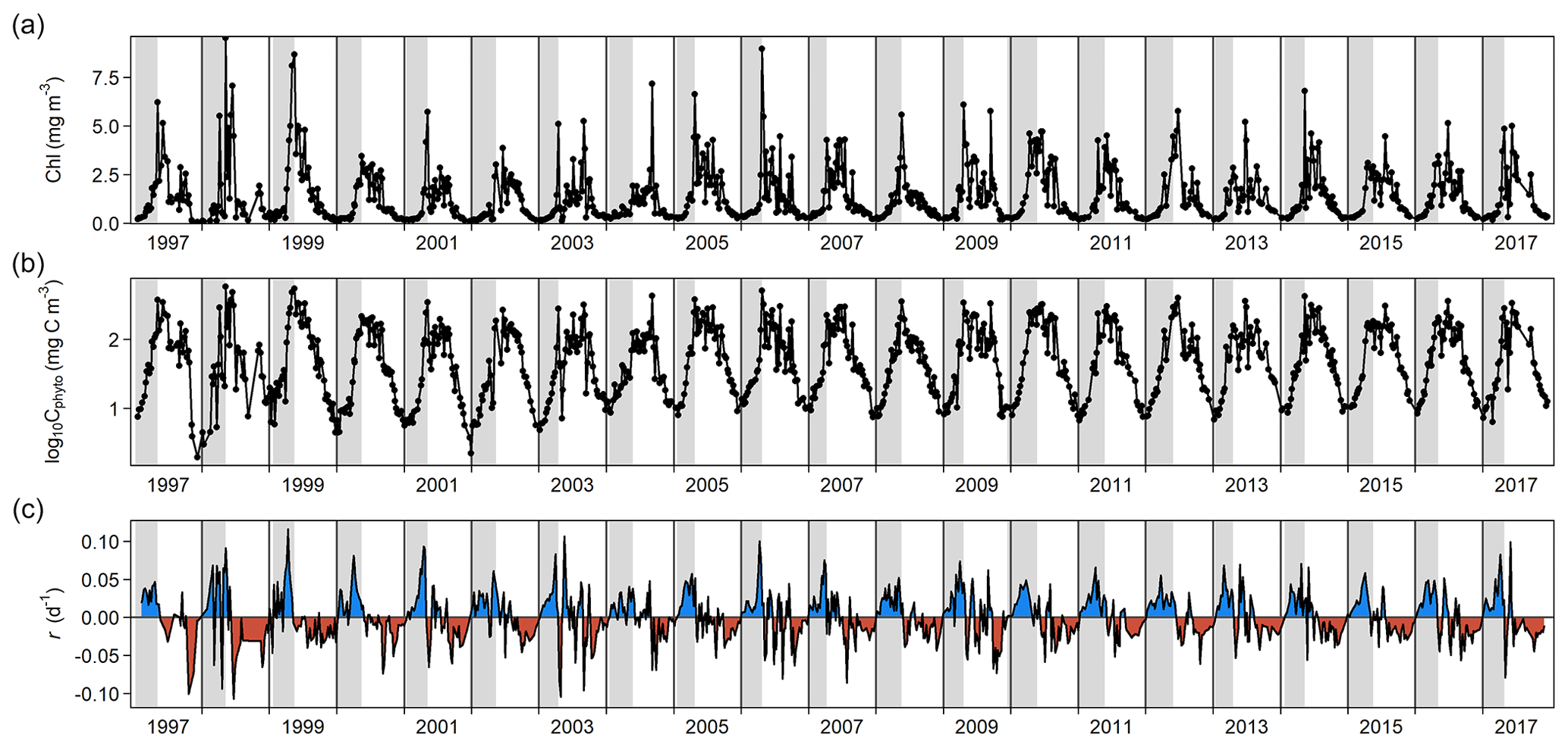
Figure 1 Changes through time in (a) chlorophyll a (Chl) concentration, (b) log-transformed phytoplankton biomass (C_phyto) concentration, and (c) biomass accumulation rate (r). Blue and red areas in (c) indicate positive and negative r, respectively. Vertical gray stripes correspond to the estimated spring bloom span each year, from t₀ to t_max C (see Methods). For 1997, we used the average date of the spring bloom onset estimated using the rest of the time series (6 January).

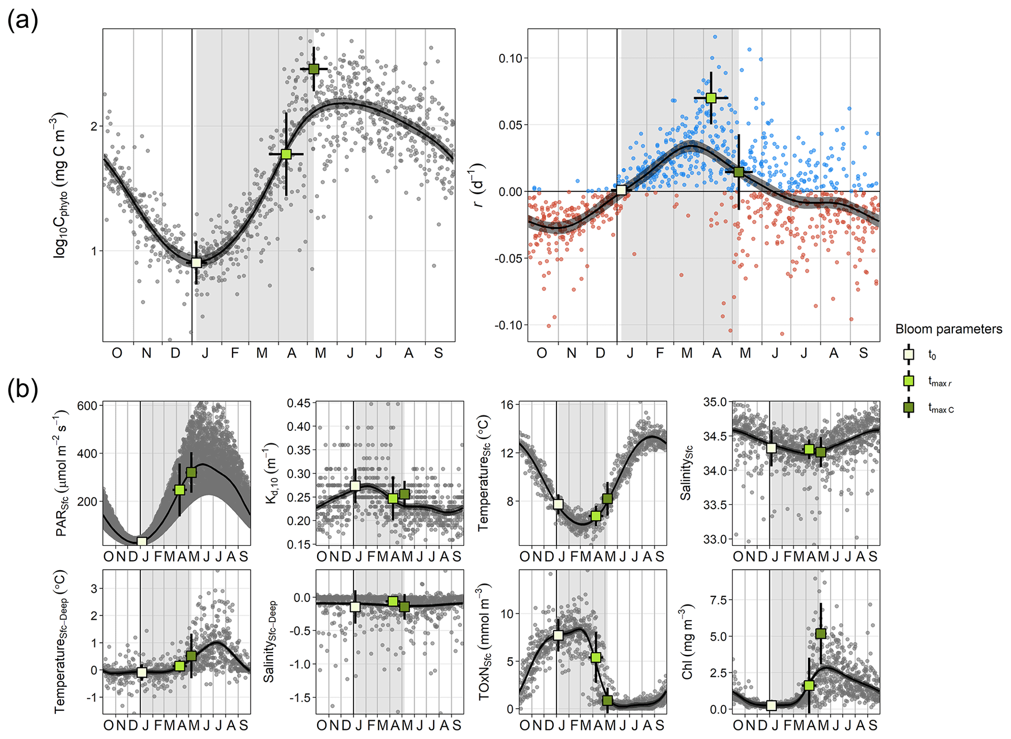
Figure 2 Seasonal cycle of physicochemical and phytoplankton variables. (a) Log-transformed phytoplankton biomass (C_phyto) concentration and biomass accumulation rate (r), which were used to estimate the timing of the spring bloom parameters: the spring bloom onset (t₀), the maximum r (t_max r), and the spring bloom peak (t_max C). (b) Surface photosynthetic active radiation (PAR), attenuation coefficient for the 0–10 m layer (K_d, 10), surface temperature and salinity (Temperature_Sfc and Salinity_Sfc, respectively), difference between surface and bottom temperature and salinity (Temperature_Sfc-Deep and Salinity_Sfc-Deep, respectively), total surface oxidized nitrogen concentration (TOxN_fc), and chlorophyll a (Chl) concentration. Dots (gray or blue and red for positive and negative r, respectively) correspond to individual values. Black curves and the associated gray shaded areas define, respectively, the average seasonality and 95 % confidence interval based on a generalized additive model (GAM). Vertical gray stripes mark the average spring bloom span. Average ± SD timing of different bloom parameters and associated average ± SD environmental conditions are also shown (squares and corresponding error bars).

Figure 3 Seasonal changes in the proportional biomass of different phytoplankton groups from 2015 to 2017. The large proportional biomass of nano-eukaryotes in October–beginning of December 2017 corresponds mainly to a Phaeocystis spp. bloom. Inner white tick marks on the x-axis indicate those dates when data were collected, and data gaps at the beginning and end of each year appear as vertical white stripes.

3.2 Effect of light on the spring bloom onset

The estimated t₀ occurred on average 16 ± 11 d after the winter solstice (Fig. 2), when surface PAR was still very low (29.34 ± 11.16 µmol m⁻² s⁻¹ on average), light attenuation was high (average K_d,10 of 0.273 ± 0.037 m⁻¹), and the water column was homogeneous (difference between surface and bottom temperature and salinity was on average −0.09 ± 0.30 ^∘C and −0.15 ± 0.25, respectively) (Fig. 2). Thus, although during the bloom onset nutrient concentrations were high (surface TOxN concentration was on average 7.71 ± 1.71 mmol m⁻³), light limitation for phytoplankton growth was at maximum in the year. Also, we observed that the r seasonal cycle increased from maximum negative rates in October–November to maximum positive ones in March–April (Fig. 2). However, for the same number of days before and after the winter solstice from November to February, average light availability and nutrient conditions were similar (Figs. 2 and 4a).

In winter, for a period extending 60 d before and after the winter solstice, we observed that r was better correlated with the rate of change in surface and attenuated PAR ($\mathrm{dPAR}/\mathrm{d}t$) than with PAR itself (Fig. 4). Specifically, we found that the proportion of variance in r explained by surface and attenuated $\mathrm{dPAR}/\mathrm{d}t$ was 0.41 and 0.50, respectively, but the proportion explained by PAR itself was almost zero. The similar effect of surface and attenuated $\mathrm{dPAR}/\mathrm{d}t$ on r indicates that, at a seasonal scale, surface PAR is the major factor driving PAR changes in time within the water column. However, Fig. 4a shows that water attenuation has a strong impact on the average light levels experienced by phytoplankton. In particular, for the period analyzed, average PAR levels assuming a homogeneous water column (PAR_Att,48) remained below 10 µmol m⁻² s⁻¹.

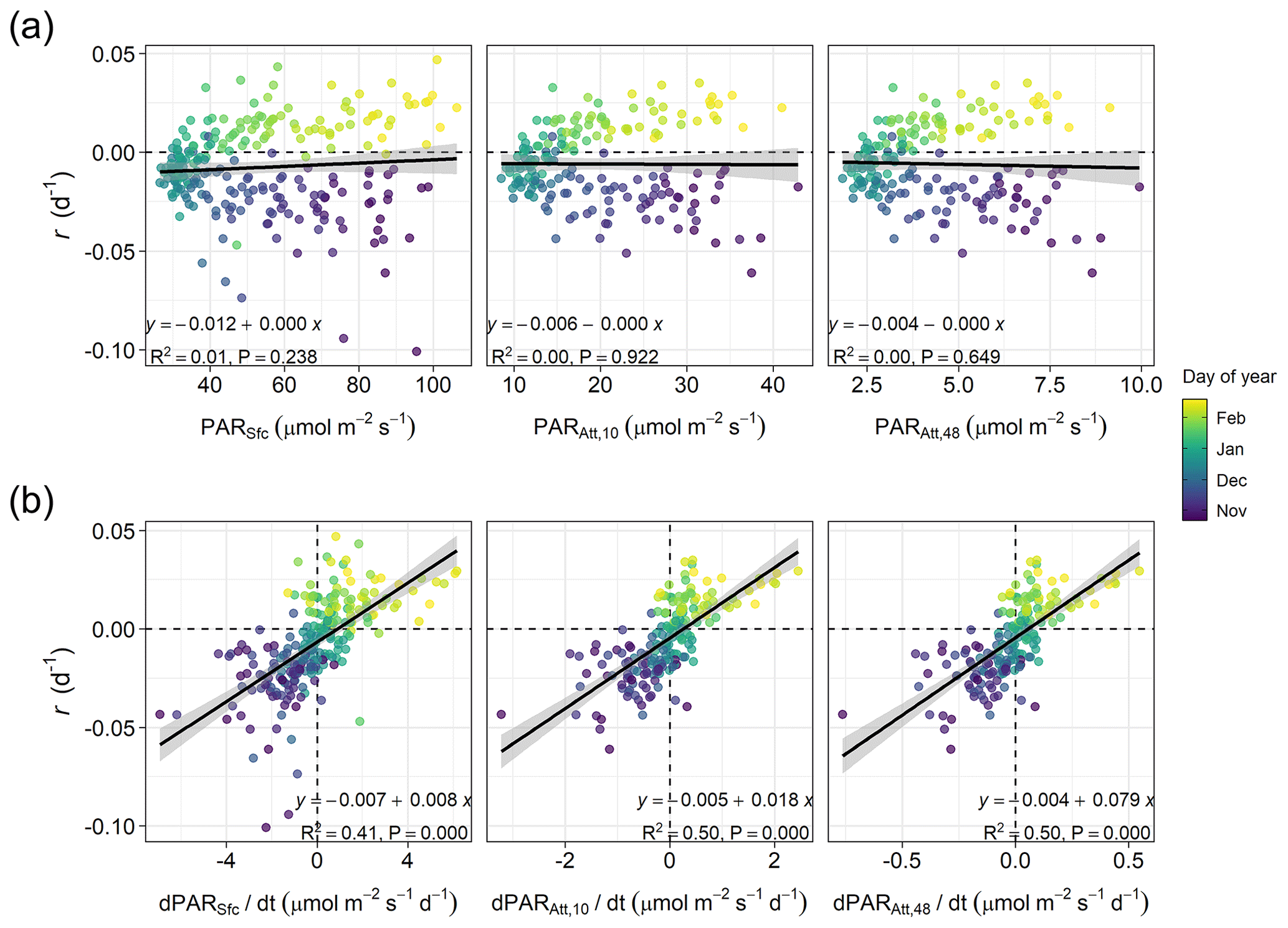
Figure 4 Linear relationships in winter (60 d before and after the winter solstice) between (a) phytoplankton biomass accumulation rate (r) and average photosynthetic active radiation (PAR) at the sea surface (PAR_Sfc), for the 0–10 m layer (the layer where phytoplankton was sampled, PAR_Att,10), or for the entire water column (i.e., 0–48 m depth, PAR_Att,48), or between (b) r and average rates of change in PAR (${\mathrm{dPAR}}_{\mathrm{Sfc}}/\mathrm{d}t$, ${\mathrm{dPAR}}_{\mathrm{Att},\mathrm{10}}/\mathrm{d}t$, and ${\mathrm{dPAR}}_{\mathrm{Att},\mathrm{48}}/\mathrm{d}t$). The shaded area represents the 95 % confidence interval associated with the estimated linear correlation (black line). The equation, proportion of variance explained (R²), and p-value (P) of the relationships are shown. Horizontal and vertical dashed lines indicate zero rates.

4 Discussion

The spring bloom onset occurred just after the winter solstice in most years at the studied coastal site. This remarkable regularity contrasts with the larger interannual variability in timing and especially in magnitude of the maximum biomass accumulation rate (r) and bloom peak biomass. The observed early winter initiation contradicts Mignot et al.'s (2018) expectations for waters without the dilution effects associated with the mixed layer deepening, indicating the operation of other processes. We found that changes from negative to positive biomass accumulation rates around the winter solstice followed seasonal variations in $\mathrm{dPAR}/\mathrm{d}t$ rather than PAR itself.

During winter, surface nutrient concentrations (as proxied by TOxN) remained high and light was probably the main limiting factor for phytoplankton growth at Stonehaven. Although this is the norm in most temperate and polar areas (Simpson and Sharples, 2012; Behrenfeld and Boss, 2014), winter light levels might be especially limiting in the Scottish North Sea due to several factors: its high latitude, storm frequency, and light attenuation due to elevated turbidity (Reid et al., 1990), which might increase in the future (Wilson and Heath, 2019). Also, the observed vertical homogeneity of the water column probably indicates an intense turbulent mixing (although see Franks, 2014), which keeps phytoplankton cells moving between surface and bottom layers, throughout the vertical light gradient (Reid et al., 1990; Simpson and Sharples, 2012). Consequently, winter PAR levels for the entire water column are well below optimal irradiances for maximum growth rates in most phytoplankton taxa (Edwards et al., 2015). Therefore, it could be surprising that the spring bloom onset usually occurred just after the winter solstice, when phytoplankton division rates (μ) suffer the strongest light limitation. Even more, r was negative during the weeks before the solstice and changed to positive some days after the solstice. Thus, r cannot just depend on μ since mean seasonal PAR levels (and probably the associated μ) are similar around the same number of days before and after the winter solstice (Fig. 4a). These observations contradict the expectations of the more traditional hypotheses about the spring bloom onset (e.g., Sverdrup, 1953).

Another consequence of the low winter light experienced by phytoplankton is that μ would be expected to respond almost linearly to changes in PAR (Edwards et al., 2015). Thus, the positive linear relationship between r and $\mathrm{dPAR}/\mathrm{d}t$ estimated around the solstice, mostly driven by seasonal changes in surface PAR, is probably reflecting the covariation of r with $\mathrm{d}\mathit{\mu }/\mathrm{d}t$. This relationship between r and $\mathrm{d}\mathit{\mu }/\mathrm{d}t$ has also been observed in oceanic waters of temperate and polar regions (see for example Behrenfeld, 2014; Behrenfeld et al., 2016; Arteaga et al., 2020) and fits within the framework of the Disturbance Recovery Hypothesis (DRH, Behrenfeld et al., 2013; Behrenfeld and Boss, 2014). Such a relationship requires a tight coupling between division and loss processes (Behrenfeld and Boss, 2018). In particular, the dynamics of small phytoplankton (<10 µm) are tightly coupled with those of microzooplankton grazers due to their fast ingestion and growth rates (Hansen et al., 1997; Haraguchi et al., 2018), allowing them to consume most phytoplankton primary production in the ocean, including coastal habitats (Calbet and Landry, 2004). Also, a Holling III functional response seems to best describe the grazing behavior of microzooplankton (Liu et al., 2021), which might be key at low winter food concentrations to allow phytoplankton biomass to accumulate (Freilich et al., 2021). At Stonehaven, we observed that small phytoplankton dominated the winter community biomass, as also occurs in other temperate oceanic and coastal areas (see for instance Haraguchi et al., 2018; Bolaños et al., 2020). This observation agrees with the expected dominance of smaller phytoplankton species when resources such as light availability are limiting, even in coastal productive environments (Marañón et al., 2012, 2015).

In addition to light variations, other factors might contribute to the observed seasonal pattern in biomass accumulation around the spring bloom onset. For instance, Rose and Caron (2007) showed that decreasing temperatures impact more negatively microzooplankton than phytoplankton maximal growth rates (i.e., measured under resource-saturated conditions, Caron and Rose, 2008; Marañón et al., 2014), which could favor the bloom initiation. In fact, Fig. 2 suggests a negative relationship between r and temperature, as confirmed through previous exploratory analyses. However, considering that phytoplankton community growth rates are temperature-insensitive under strong light limitation (Marañón et al., 2014; Edwards et al., 2016) and that very low chlorophyll concentrations might even reverse the expected relationship between the proportion of phytoplankton production grazed by microzooplantkon and temperature (Chen et al., 2012), we hypothesize a lesser role of temperature than light variations. Nevertheless, the contribution of temperature to the observed seasonality around the onset of biomass accumulation has to be further investigated. Also, the southward coastal flow characteristic of the study area (Holt and Proctor, 2008; León et al., 2018) could contribute to the bloom onset delay with respect to the winter solstice (16 d on average) by bringing waters with lower phytoplankton biomass concentrations. This could occur in winter as the further north the spring bloom occurs in the North Sea, the longer it takes to reach a certain biomass level (Henson et al., 2009). Additionally, although we analyzed the spring bloom as an aggregate community phenomenon, we recognize the importance of the seasonal phytoplankton succession (Lewandowska et al., 2015). In particular, we hypothesize that to keep μ accelerating in response to the seasonal light improvement, it is necessary that a succession of species with traits suited to each new environmental condition occurs during the bloom progression (Behrenfeld et al., 2016, 2021a, b), consistent with the complex changes in group composition observed (Fig. 3).

One limitation of our study is using an average seasonality of C : Chl ratios to estimate phytoplankton biomass for all years, as these ratios change in response to environmental conditions (Geider, 1987). Alternatively, some studies have proposed models that calculate C : Chl based on environmental conditions (e.g., Geider, 1987; Cloern et al., 1995). This approach is not possible in our case as we cannot determine the mixed layer depth in summer and, consequently, the amount of light experienced by surface phytoplankton. Nevertheless, for the winter period analyzed, when the active mixing usually extends the entire water column, biomass estimated assuming a homogeneous water column and using C : Chl models (Geider, 1987; Cloern et al., 1995) were very similar to those calculated using a constant C : Chl seasonality (Fig. S6). Also, measuring PAR in situ would have improved the accuracy of our PAR estimations. However, we think our results were not importantly affected by this, as we were mainly interested in the seasonal pattern around the spring bloom onset. Additionally, our study location belongs to an area where strong winds and tidal currents mix and homogenize the environment, allowing only intermittent stratification in summer (Pingree and Griffiths, 1978; Van Leeuwen et al., 2015). The Stonehaven site is often taken to be representative of this area of the Scottish coastal North Sea, identified as a distinct hydrodynamic region (Van Leeuwen et al., 2015). Nevertheless, advective processes such as the mentioned southward coastal flow (Holt and Proctor, 2008; León et al., 2018) could still create some heterogeneity in the region. Disentangling local from larger-scale processes is then crucial to deeply understand the intra- and interannual variability of the whole spring bloom in this complex hydrographic ecosystem (Blauw et al., 2018). This could be achieved through Lagrangian studies and dynamic 3-D models that consider advection and incorporate processes at very different spatiotemporal scales.

5 Conclusions

Overall, we showed that the spring bloom onset in a generally well-mixed coastal location of the North Sea supports the Disturbance Recovery Hypothesis (DRH). Nevertheless, the mechanisms described in other competing hypotheses such as the Critical Depth Hypothesis (Gran and Braarud, 1935; Sverdrup, 1953) or the Critical Turbulence Hypothesis ( Huisman et al., 1999) might contribute to the spring bloom development (Lindemann and St. John, 2014; Chiswell et al., 2015). For instance, a water column stratification due to the surface heating or a relaxation of the turbulent mixing caused by weak or calm winds can lead to fast (albeit temporary) increases in both light availability and division rates (Morison et al., 2019, 2020; Mojica et al., 2021), as described for oceanic waters by Mignot et al. (2018) and Yang et al. (2020). Our results suggest that the DRH might also explain the spring bloom onset in other coastal areas or lakes, and that this onset can occur in early winter despite the absence of a mixed layer deepening.