the Creative Commons Attribution 4.0 License.
the Creative Commons Attribution 4.0 License.
 | 18 May 2022
Global nutrient cycling by commercially targeted marine fish
Priscilla Le Mézo
Jérôme Guiet
Kim Scherrer
Daniele Bianchi
Eric Galbraith
Throughout the course of their lives fish ingest food containing essential elements, including nitrogen (N), phosphorus (P), and iron (Fe). Some of these elements are retained in the fish body to build new biomass, which acts as a stored reservoir of nutrients, while the rest is excreted or egested, providing a recycling flux to water. Fishing activity has modified the fish biomass distribution worldwide and consequently may have altered fish-mediated nutrient cycling, but this possibility remains largely unassessed, mainly due to the difficulty of estimating global fish biomass and metabolic rates. Here we quantify the role of commercially targeted marine fish between 10 g and 100 kg () in the cycling of N, P, and Fe in the global ocean and its change due to fishing activity, by using a global size-spectrum model of marine fish populations calibrated to observations of fish catches. Our results show that the amount of nutrients potentially stored in the global pristine biomass is generally small compared to the ambient surface nutrient concentrations but might be significant in the nutrient-poor regions of the world: the North Atlantic for P, the oligotrophic gyres for N, and the high-nutrient, low-chlorophyll (HNLC) regions for Fe. Similarly, the rate of nutrient removal from the ocean through fishing is globally small compared to the inputs but can be important locally, especially for Fe in the equatorial Pacific and along the western margin of South America and Africa. We also estimate that the cycling rate of elements through biomass was on the order of 3 % of the primary productivity demand for N, P, and Fe globally, prior to industrial fishing. The corresponding export of nutrients by egestion of fecal matter by was 2.3 % (N), 3.0 % (P), and 1 %–22 % (Fe) of the total particulate export flux and was generally more significant in the low-export oligotrophic tropical gyres. Our study supports a significant, direct role of the fraction of the ichthyosphere in global nutrient cycling, most notably for Fe, which has been substantially modified by industrial fishing. Although we were not able to estimate the roles of smaller species such as mesopelagic fish because of the sparsity of observational data, fishing is also likely to have altered their biomass significantly through trophic cascades, with impacts on biogeochemical cycling that could be of comparable magnitude to the changes we assess here.
- Article
(9125 KB) - Full-text XML
-
Supplement
(3465 KB) - BibTeX
- EndNote


Nutrient elements are used by organisms to construct the molecules they need to grow and metabolize but are often scarce, limiting growth rates (Moore et al., 2013; Sterner and Elser, 2002). Plankton and bacteria dominate the cycling of nutrients in the ocean (Sarmiento and Gruber, 2006), but an increasing number of studies recognize the contribution of animals to biogeochemical cycles (e.g., Wilson et al., 2009; Bianchi et al., 2013; Saba et al., 2021). Locally, it has been shown that marine animals can significantly impact the supply and storage of nutrients with consequences for primary production (Cavan et al., 2019; Roman et al., 2014) and interact with the cycling of elements through direct and indirect pathways (Vanni, 2002; Atkinson et al., 2017; Allgeier et al., 2017). For instance, Leroux and Schmitz (2015) described a theoretical framework in which animals control the flux of nutrients up the trophic chain through predation and release of waste products while also affecting the cycling of nutrients through non-consumptive effects (e.g., prey selection and stress induced in prey). In addition, since animals can swim and move in the water column, they are also able to transport nutrients from one place to another, over distances that increase with animal size (Hall et al., 2007; Vanni, 2002; Roman et al., 2014). But thus far there has been little effort to estimate how the global fish population, which we term “ichthyosphere”, influences large-scale nutrient cycling in the ocean.
During their life cycle, fish assimilate, store, and recycle essential elements that they need to build their body tissues. This storage of nutrients within fish biomass is important for human nutrition as wild-caught fish globally provide essential proteins and other micronutrients (Hicks et al., 2019). Apart from a dietary interest for humans, the reservoir of nutrients comprised by fish biomass can play a role in ecosystem function as a nutrient stockpile, the importance of which depends on how much nutrients are available otherwise (Allgeier et al., 2016). For example, the nutrients embedded in fish biomass are not directly available for primary producers, which can appear as a type of competition for resources (Hjerne and Hansson, 2002). But at the same time, the cycling of elements by fish acts as a source of nutrients to primary producers, as fish recycle elements through the excretion of dissolved bioavailable components.
The cycling of N and P by fish has often been studied in freshwater systems, but little is known for the global ocean (Schindler and Eby, 1997; Vanni, 2002; Vanni et al., 2006; Griffiths, 2006). For instance, McIntyre et al. (2008) showed that fish are able to create hotspots of recycled nutrients in streams that could meet more than 75 % of the algal and microbial requirement for N, and Allgeier et al. (2014) showed that fish are a fundamental nutrient source to coral reefs. Additionally, fish egest particulate products that can be mineralized and enhance productivity or that can sink to depth and export elements (Davison et al., 2013; Saba and Steinberg, 2012), so that they are no longer available for primary producers. As such, fish biomass can act as a bank account for nutrients, depositing nutrients when fish are feeding rapidly and withdrawing nutrients to the water column when metabolism exceeds predation. Finally, the egestion of particulate products by fish has been shown to modify the stoichiometry of biogenic particles, including dramatic changes of Fe : C, implying that egested material may also modify the relative availability of nutrients through the water column (Le Mézo and Galbraith, 2020).
The amount of nutrients stored and cycled by fish can vary with different environmental and physiological factors, in space and time (e.g., Halvorson and Small, 2016; Prabhu et al., 2016; Francis and Côté, 2018; Czamanski et al., 2011; Allgeier et al., 2014). In addition to natural variations, anthropogenic activities, mostly fishing, modify the storage and cycling of nutrients by the ichthyosphere. For instance, Layman et al. (2011) and Allgeier et al. (2016) analyzed the cycling of N and P by fish in fished and un-fished coastal sites of the Bahamas and the Caribbean, respectively. Layman et al. (2011) showed lower recycling rates of nutrients by fish in fished sites, due to biomass reduction and habitat fragmentation. Beyond fish biomass reduction, Allgeier et al. (2016) stressed the role of community size structure that, influenced by fishing, also led to reduction in nutrient storage and cycling.
Although numerous works have identified significant local effects, little is known about the contribution of the ichthyosphere to nutrient budgets at the global scale. Maranger et al. (2008) used global fish catch data to estimate the total removal of N by commercial fisheries. They integrated a spatial component in their analysis by computing N removal in 58 large marine ecosystems (LMEs) and compared it to fertilizer runoff in each off these LMEs. Moreno and Haffa (2014) took a similar approach to estimate the amount of Fe removed each year by fishing from 1950 to 2010. They also used biomass estimates from literature to quantify the amount of Fe in the global fish biomass and the amount of Fe cycled by this biomass each year. However, the total inventories and cycling rates have remained unquantified due to the lack of reliable global fish biomass and metabolism estimates.
Recently Bianchi et al. (2021) used a dynamical global model of marine commercially targeted fish (CTF), constrained by observed fish catches, to estimate the total CTF biomass and cycling rates and their distribution in the world's oceans. Our study builds on Bianchi et al. (2021) by using an updated version of the model to estimate the role of CTF in the global cycling of the three most important growth-limiting nutrients: N, P, and Fe (Fig. 1). Section 2 lays out the method we use to investigate the nutrient dynamics for the total CTF biomass for body sizes between 10 g and 100 kg, hereafter , using model simulations for both a reconstructed state prior to industrial fishing (“pristine”) and a simulated global peak catch. We then present and discuss the results as a series of relatively self-contained sections by topic. Section 3 details the total nutrient content in , Sect. 4 focuses on nutrient cycling rates by , Sect. 5 discusses an extension of the estimates to all fish from 1 g to 1000 kg, and Sect. 6 presents the impact of fishing on (Fig. 1). Section 7 concludes the paper.
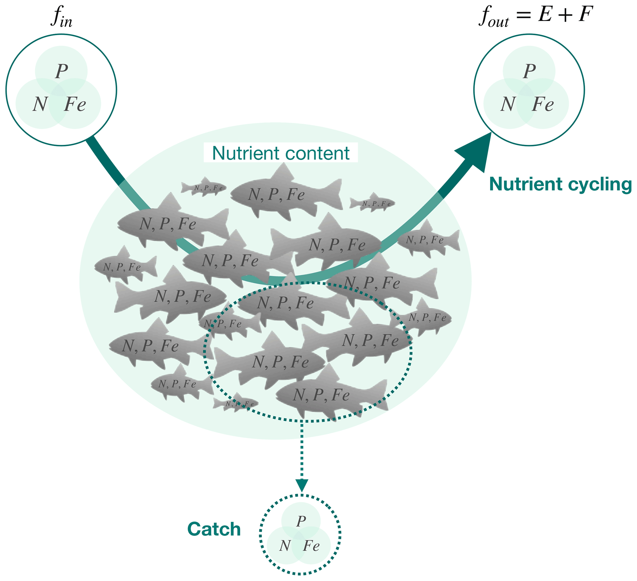
Figure 1The ichthyosphere role in global nutrient cycling. The diagram schematically indicates the cycling of nutrients (N, P, and Fe) through the global fish biomass (solid arrow), the nutrients contained within the biomass, and the removal of nutrients from the ocean through fishing (dashed arrow). fin and fout are the fluxes in and out of the global fish biomass, respectively. E indicates excretion (release of dissolved compounds), and F indicates egestion (release of solid feces).
2.1 Model description and simulations
We used an ensemble of simulations from the BiOeconomic mArine Trophic Size-spectrum (BOATS) model (Carozza et al., 2017), also used by Bianchi et al. (2021).
2.1.1 The model
BOATS provides a global, size-based numerical simulation of commercially targeted marine organisms (including molluscs and crustaceans, here collectively termed “fish”) by coupling an ecological module with a fishery economics module (Carozza et al., 2016, 2017). The ecological model is based on processes derived from macro-ecological theory (Carozza et al., 2016), parameterized through a Bayesian Monte Carlo approach that optimizes model performance by minimizing the discrepancy between observed and simulated catch and biomass for globally distributed LMEs (Carozza et al., 2017). Modeled fish are divided into three “super-species” groups defined by the asymptotic mass of fish: small (0.3 kg), medium (8.5 kg), and large (100 kg). Individual sizes are binned logarithmically into 30 mass classes ranging from 10 g to 100 kg, with all three size groups starting at 10 g (Carozza et al., 2016). The three groups are not intended to represent the entire marine ecosystem but rather the sum of all species that have been commercially harvested (and are therefore accounted for in harvest records and stock assessments, which are used to constrain the model). The underlying philosophy of the model is that, although these very diverse species differ widely in their biological strategies, all are competing for food energy ultimately provided by the fixation of organic carbon through photosynthesis (which has been shown to limit fish harvests; Chassot et al., 2010; Stock et al., 2017), while inhabiting the same environment, which therefore makes them subject to the same basic ecological constraints. The constraints we apply in the model are the impacts of water temperature on growth, mortality, and phytoplankton size, and net primary production. Although this biologically “coarse-grained” approach precludes resolution of species-level dynamics, it is solidly founded in bioenergetic principles and is well-suited to providing a global view of the entire ecosystem on long timescales, given that it is likely to be relatively robust under any changes in the distribution, abundance, or evolution of commercial stocks under historical fishing pressure (Guiet et al., 2020). Figure 2 provides a schematic overview of the model structure.
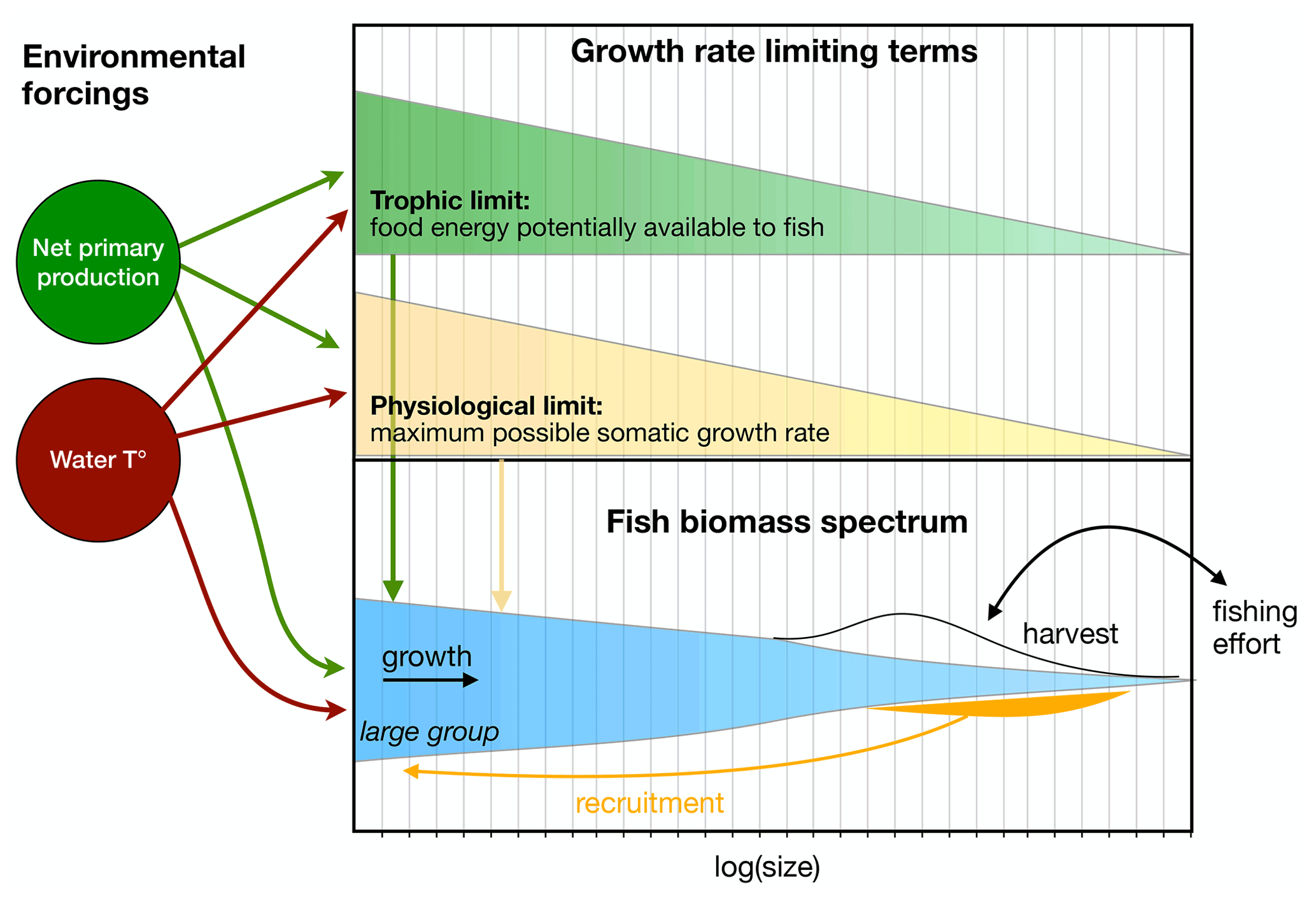
Figure 2Schematic overview of the BOATS model. The red, green, and black arrows indicate dependencies of model components on external forcings. The top panel indicates the energetic limits of growth as a function of fish size, while the bottom panel illustrates the three size spectra of fish groups (for simplicity only the large group is represented), their internal dynamics, and the link to economics via harvest and the interactive effort.
The BOATS model was deliberately developed to represent marine organisms over the size range most heavily targeted by fisheries, since this is the range for which fishery data can offer useful constraints on the ecosystem function (Carozza et al., 2016, 2017). The starting point of 10 g coincides roughly with the weight of mature anchovy (approximately 11 cm in length according to Pauly and Tsukayama, 1984), while above 100 kg the growing significance of mammals in the ocean makes a strictly ectothermic model less capable of capturing the full marine animal community (Hatton et al., 2021).
Fishing effort and catch are computed assuming open-access dynamics and based on the Gordon–Schaefer fishery economics model (Gordon, 1954; Schaefer, 1954) with increasing catchability over time due to technological progress (Galbraith et al., 2017).
The model represents fish on a two-dimensional grid, i.e., longitude and latitude, which is divided in regular 1∘ × 1∘ grid cells. Thus, the model does not resolve the vertical dimension but sums all ecosystem productivity and biomass within the water column at each horizontal point. Given that the model does not resolve interactions in space between individuals, this reduction in dimensionality does not – on its own – introduce any bias. The model is forced by monthly climatologies of observed net primary production and surface ocean temperature (Dunne et al., 2007).
Galbraith et al. (2019) hypothesize that fish growth is reduced under iron scarcity in the wild and demonstrate that the implementation of a simple form of iron limitation of fish in BOATS improves the simulated fish catch in oceanic regions known to have low iron concentrations. We thus used a different version of the model from Bianchi et al. (2021) that includes an Fe limitation of fish growth, using surface nitrate concentrations as a proxy for iron limitation as described in Galbraith et al. (2019).
2.1.2 Simulations
We use the parameter sets selected in Bianchi et al. (2021) to run our updated Fe-limited model version. Briefly, from the Monte Carlo ensemble of 10 000 simulations, Bianchi et al. (2021) selected the parameter combinations (31 in total) that best match the historical catch maxima across LMEs as reconstructed by the Sea Around Us Project (SAUP) (Pauly and Zeller, 2016), while simultaneously falling within the acceptable bounds for the catch-to-biomass ratio as constrained by stock estimates (Ricard et al., 2012). We then perform simulations with our Fe-limited version of the model using these 31 model parameter combinations. Each simulation includes 200 years without catch to estimate pristine biomass at equilibrium, followed by 220 years with fishing driven by the only increase in the catchability of biomass at 7 % yr−1 to reproduce the historical progression of the global fishery (Galbraith et al., 2017). The simulations slightly underestimate the observed LME catch peak of ∼ 110 Mt yr−1, and the variation between LME peaks corresponds to observation with a squared Pearson product-moment correlation coefficient r2=0.42, p value , when averaged across all ensemble members (Figs. S1 and S2 in the Supplement). More details on the observational constraints and on the Monte Carlo approach used here can be found in Bianchi et al. (2021). From the 31 simulations of the ensemble, we analyze the global biomass and cycling rates at pristine state and at the time of the global peak catch.
2.2 Nutrient content of fish
To estimate the quantity of a nutrient X stored in fish biomass, we convert our modeled biomass estimates from wet weight to carbon (C) weight and multiply by an average mass ratio of nutrient to carbon, X : C. Prior work has suggested that body nutrient concentration of fish may be affected by several factors such as body size, ontogeny, species, sex, diet, temperature, or water nutrient concentration (e.g., Halvorson and Small, 2016; Prabhu et al., 2016; Allgeier et al., 2017), with species appearing to be the most important factor (Allgeier et al., 2020). Among these factors, our model could potentially account for change during ontogeny as organisms grow in size, but analysis of the available data (see Supplement) shows little to no systematic variation in specific nutrient content with size. We thus assumed constant nutrient proportions throughout food webs.
Although the model implicitly includes molluscs and crustaceans, they represent only a small proportion of the commercial catch between 10 g and 100 kg (from SAUP data invertebrates comprised about <14 % of total catch). Additionally, the measured nutrient content of molluscs and crustaceans falls within the uncertainty range around the mean value for fish (Tables S2–S3 in the Supplement). As a result, we did not attempt to account for invertebrates separately, but we applied the fish nutrient ratios to all biomass. The Fe content of fish is poorly constrained (few whole body measurements), so we rather use the 95 % confidence interval from available data, which ranges between 10 and 200 µmol Fe (mol C)−1 (Galbraith et al., 2019).
2.3 Nutrient cycling by fish
First, we define the terms we use by considering the fate of a nutrient element when ingested by an individual fish (Fig. 3a). A fish i ingests a mass flux of a nutrient, Ii (e.g., g N d−1), of which a fraction α (between 0 and 1) is absorbed across the gut to produce an absorption flux, Ai, while the remainder is egested in the form of feces, (Fig.3). Note that absorption efficiency here is defined as the difference between ingestion and egestion. Published estimates of absorption efficiencies of fish are listed in Table 1. A fraction of the element absorbed across the fish gut is then used for growth and reproduction, , where γ is the somatic assimilation efficiency. The trophic efficiency, τ, is commonly defined as the ratio of the production of new biomass to the ingestion rate and is equal to γα. The remainder is used for maintenance and excreted back to the water; (Fig. 3a, b). We define the cycling rate of a nutrient through the fish as , which can be thought of as the biologically processed outputs of the fish.
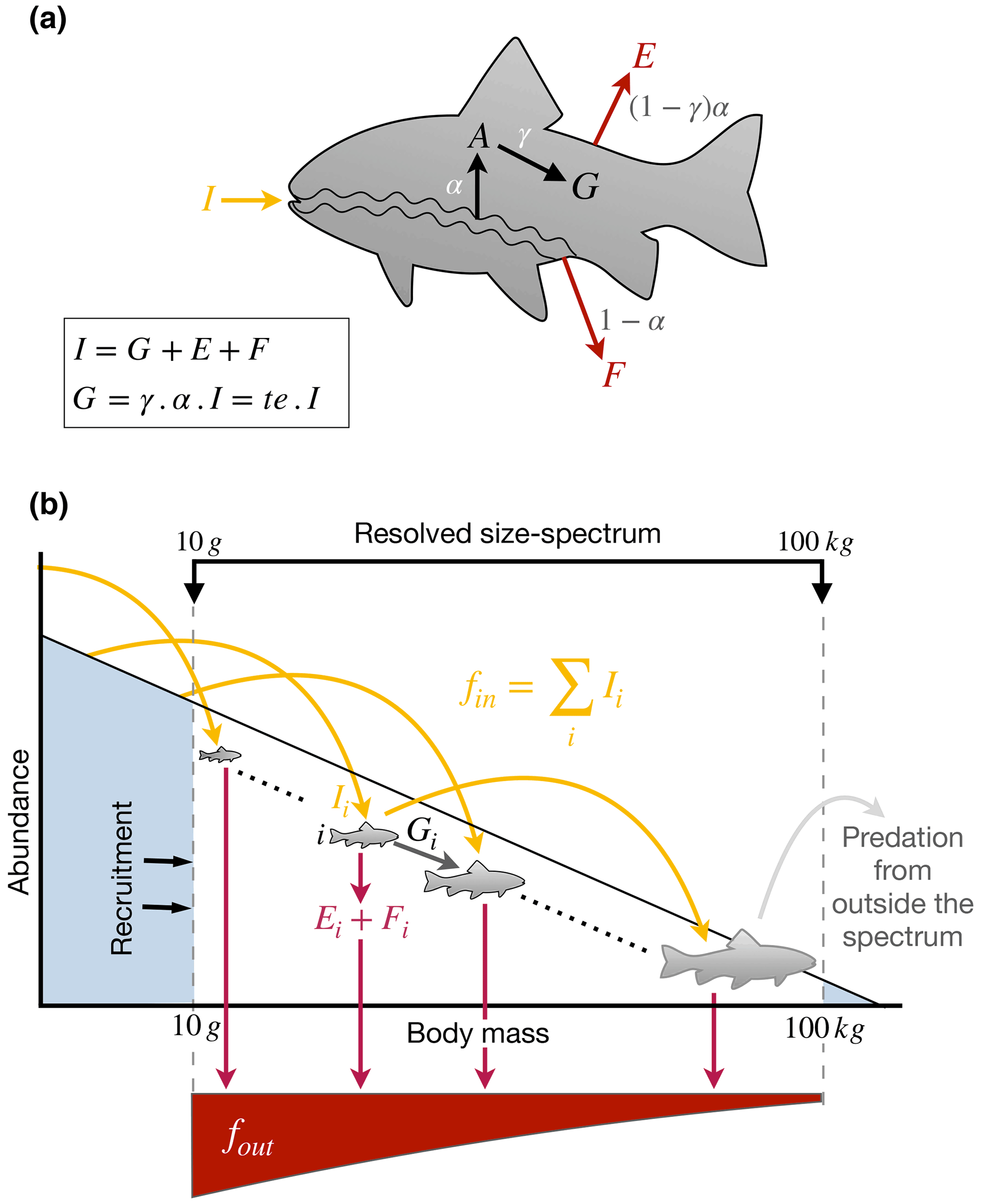
Figure 3Schematic of the flow of elements (a) within an individual and (b) through the size spectrum. I: ingestion; G: growth and reproduction; A: absorption; E: excretion; F: egestion (feces); α: absorption efficiency, i.e., assimilation efficiency net of egestion; γ: somatic assimilation efficiency, i.e assimilation allocated to growth; fin: flux entering the spectrum; fout: flux going out of the spectrum.
Table 1Mean nutrient content in fish, zooplankton, and phytoplankton and mean absorption efficiencies (A) of N, P, and Fe for fish used in this study.

Data from a Czamanski et al. (2011) (percent converted back to wet weight using a 25 % dry weight in wet weight (Galbraith et al., 2019), geometric mean, and P absorption efficiency computed from the linear regression between predator and prey C P ratio). b Schindler and Eby (1997). c Galbraith et al. (2019). d Thodesen et al. (2001). e Prabhu et al. (2016). f Moore et al. (2013). “ww” is for wet weight, Fe-poor and Fe-rich refer to the conditions in which the organisms lived, and low/high are the low and high estimates from gathered data in Galbraith et al. (2019). Standard deviations are the arithmetic standard deviations, associated with the arithmetic mean. Ratio mean values are geometric means, and the ranges are the 95 % confidence interval, except for fish Fe : C for which the range is estimated from Galbraith et al. (2019).
Based on these terms, we follow Bianchi et al. (2021) to estimate the total flux of carbon through the based on the community average τ and growth rates Gi(C) of all simulated fish within the size spectrum. We calculate the ingestion for each fish within the size bins by dividing Gi(C) by τ(C) (which is 0.17 when averaged across the ensemble). We then subtract the growth Gi(C), to arrive at the carbon cycling rate, and sum over all fish (Fig. 3b). We note that at steady state for the community level there is no net growth since new production is balanced by predation, but by subtracting Gi(C) we ensure that there is no double-counting of internal cycling within the simulated size spectrum through predation on simulated fish. Because the model mean predator–prey mass ratio for the ensemble is 0.6 × 10⁴, there is very little predation within the resolved size spectrum (there are only 4 orders of magnitude across the smallest to the largest size bin), so that the subtraction of Gi(C) could lead to a small systematic underestimate in our cycling estimates. However, we also consider that predation by large predators not resolved by the model, including very large fish, marine mammals, or birds, will cause a portion of the resolved fish growth to be cycled by other organisms outside of the . Any consequent underestimate is therefore likely to be significantly less than the value of τ(C) (i.e., significantly less than 17 %).
Thus, our carbon cycling rate equation for is given by the output flux equation:
We can then use the input rate of carbon to the fish population, fin(C), to calculate the cycling terms for any nutrient element based on the stoichiometry of the ingested organic matter and element-specific absorption. We do so by taking the nutrient X-to-carbon mass ratio within the prey, (X : C)prey, and the absorption efficiency of nutrient X, αX, to compute
where fin(X) is the ingestion flux of nutrient X into all fish, and E(X) and F(X) are the excreted and egested fluxes of nutrient X, respectively, for all fish.
Note that we separate the ingested fraction, I, and egested fraction, F, using a constant mean absorption coefficient for each nutrient, αX (Table 1).
As indicated by Eq. (2), the cycling rate we calculate for an element X will be proportional to the average value of (X : C)prey. To maintain tractability, we assumed that zooplankton provide a representative indication of the stoichiometry of the fish food source, and we used mean zooplankton N and P nutrient content to compute the cycling of these elements through the fish biomass (Table 1). For zooplankton Fe content, spatial variability appears to be more important than for N and P, given significant differences between Fe-rich and Fe-poor regions (Table 1; Galbraith et al., 2019). In order to be thorough, we computed Fe cycling in three different ways based on the various computation of the Fe : C distribution of zooplankton: (1) we used a mean Fe : C in zooplankton of 30.6 µmol Fe (mol C)−1, (2) we used a spatial variation between Fe-rich and Fe-poor regions and used the Fe : C mean values in Fe-poor and Fe-rich regions, respectively, from Table 1, and (3) we used the same spatial variation, but with the low and high Fe : C estimates of zooplankton from Table 1. For the spatial variations in Fe : C, we assumed that Fe-poor conditions are encountered in HNLC regions, which are determined by a concentration of surface nitrate larger than 5 mmol N m−3. In order to take into account the gradient between these regions, we locally weighted zooplankton Fe content using a Michaelis–Menten function.
2.4 Primary producer demand, nutrient concentrations, export, and atmospheric deposition
We compare the nutrient cycling by fish to the nutrient demand by primary producers, in order to provide a rough characterization of its magnitude. We use an averaged satellite-based primary productivity (PP) (Dunne et al., 2007) to compute the PP demand for N, P, and Fe. We predict the C : P and C : N ratios in phytoplankton using empirical relationships with and surface concentrations as described in Galbraith and Martiny (2015):
where nutrient concentrations are in µmol L−1.
Similarly to zooplankton, the Fe : C of phytoplankton is computed by allowing variation in stoichiometric ratios between the mean value found in Fe-poor conditions and the mean value found in Fe-rich conditions, or between the high and low phytoplankton Fe : C estimates (Table 1), using a Michaelis–Menten equation analogous to Eq. (3).
We then use the phytoplankton nutrient ratios to compute the export of nutrients from a satellite-based estimate of total C export (Dunne et al., 2007).
We use the World Ocean Atlas-observed and water concentrations (Garcia et al., 2013) and dissolved Fe concentrations simulated by the biogeochemical model TOPAZ2 (Dunne et al., 2013) to compare the fish biomass nutrient content to the surface ocean ambient concentrations of nutrients and to compute the stoichiometric ratios (e.g., in Eq. 4). The TOPAZ2 model represents the cycles of different elements from carbon to calcite and Fe with 30 different tracers and the dynamics of three groups of phytoplankton. Surface concentrations are computed using the 2002–2019 annual mean euphotic depth from Aqua MODIS (2018).
Finally, we compare the rate of nutrients removal by fishing at the time of global peak catch to current atmospheric deposition fields of soluble N (Brahney et al., 2015) and Fe (Mahowald et al., 2009) (Fig. S3). The catch rate and its spatial distribution are simulated by the coupled economic–ecological model and systematically differs from the actual historical peak in that the model ensemble simulates higher catch rates in the open ocean than observed.
Our results show that the nutrients contained within biomass represent a non-negligible proportion of the ambient dissolved concentrations in areas where these concentrations in seawater are low and/or where biomass is high. The highest amounts of N, P, and Fe in the pristine fish biomass are located in the most productive regions along the coasts, where most simulated fish biomass occurs (Fig. 4a). Globally, the estimated pristine biomass of , which represents 2.5±0.8 Gt of wet biomass, contains 69±31 Tg of N, 15±14 Tg of P, and 0.012–0.23 Tg of Fe, of which about half is found in the large marine ecosystems (LMEs) (Table 2). Note that, in our computations, fish biomass is the only term that varies spatially since the nutrient contents of fish, (X : C), are held globally constant (see Methods section).
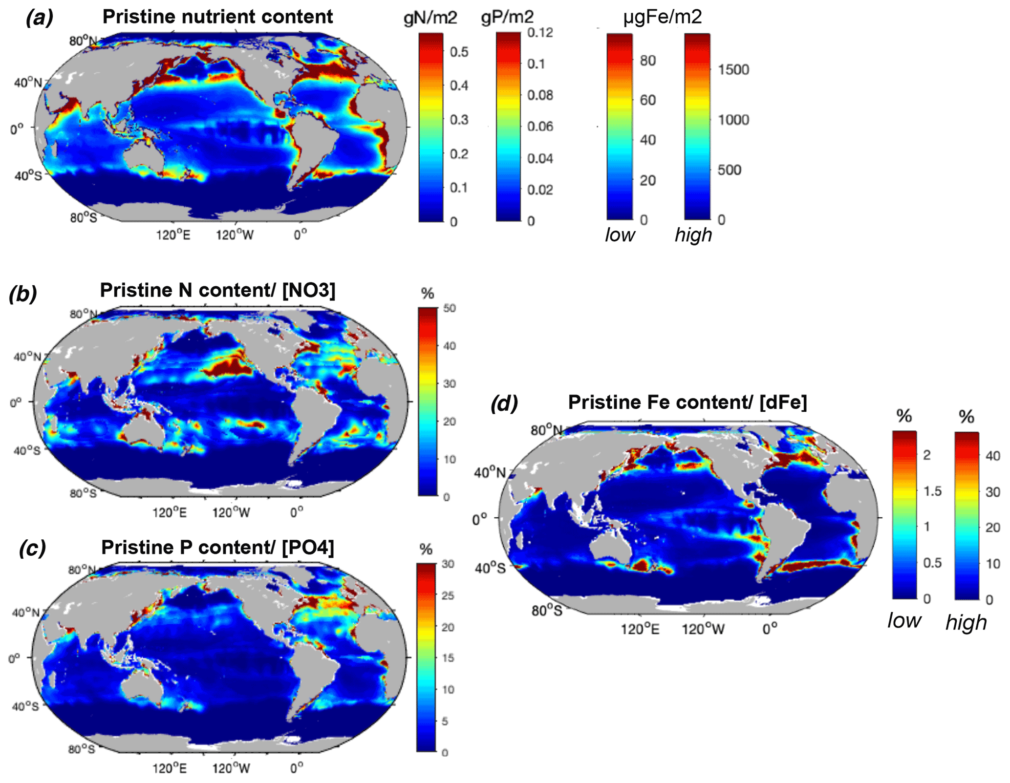
Figure 4Modeled commercial pristine fish biomass mean nutrient content and relative to surface nutrient concentrations. (a) P content (mmol P m−2), N content (mmol N m−2), and Fe content (low and high estimates, µmol Fe m−2) of the global pristine biomass, and (b) N content relative to surface concentrations (%), (c) P content relative to surface concentrations (%), and (d) Fe content (low and high estimates) relative to modeled surface dissolved Fe (%) from the TOPAZ model (Dunne et al., 2013). All surface concentrations are integrated over the 2002–2019 annual mean euphotic depth (Aqua MODIS, 2018). The N, P, and Fe content of fish is represented on a single map given that we used a globally constant nutrient ratio for each element, so that all spatial variation is caused by fish biomass.
Table 2Table of values in LMEs from the model ensemble simulations in the pristine state and at the global peak catch. This table contains integrated values of nutrient content in biomass (Tg) and the ratio of nutrient content in biomass with surface nutrient concentrations (%).
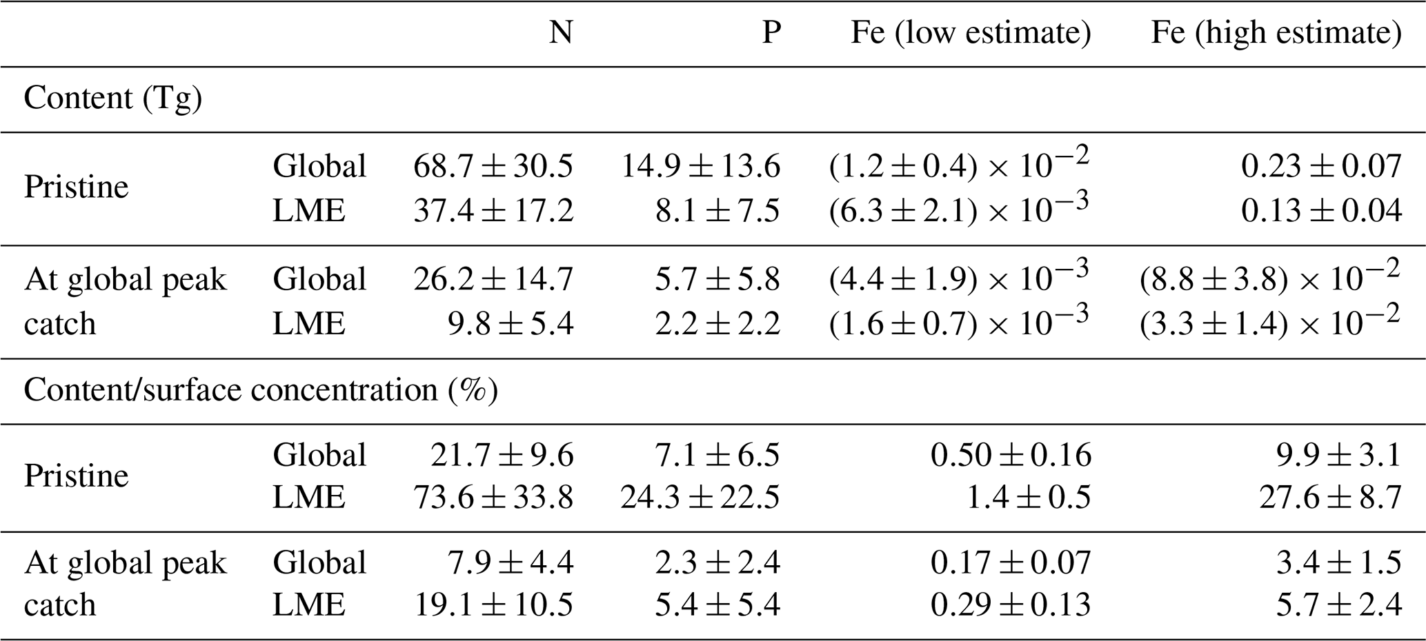
The N content of biomass is locally on the same order of magnitude as ambient surface concentrations, exceeding 50 % of in the oligotrophic gyres where nutrient concentrations are low and in coastal shelves where large fish biomass accumulates prior to industrial fishing (Fig. 4b, Table 2). The amount of P in biomass represents a high proportion of available in the North Atlantic Ocean, which is relatively P-poor, exceeding 30 % in some areas (Fig. 4b). The ratio also exceeds 20 % in the western North Pacific and in a few locations such as in the Arabian Sea. biomass stores much higher Fe compared to dissolved surface concentrations in the highly productive subtropical front waters of the North Pacific, North Atlantic, and Southern oceans, with relative values exceeding 50 % for the high-end estimate (Fig. 4d). Despite low surface Fe concentrations in the Southern Ocean, the proportion in is particularly low due to the low modeled fish biomass, while in the tropical Atlantic the input of Fe from dust greatly overwhelms the iron in fish (Mahowald et al., 2009; Myriokefalitakis et al., 2016).
In summary, the storage of nutrients by biomass can be quite significant, compared to the dissolved nutrient inventory of the euphotic zone, but only where ambient dissolved nutrient concentrations are low and/or fish biomass is high. In these areas, biomass could be expected to have a greater potential as a source (if stored nutrients are made available) or a sink (if the nutrients cannot be used by primary producers) of nutrients.
3.1 Comparison to previous estimates
Our estimates for the N and Fe contents of the ichthyosphere differ from previous studies to some degree, which can be explained by differences in the estimates of global fish biomass and/or uncertainty regarding fish nutrient contents (we were not able to find prior estimates for P).
The amount of N stored within the global fish biomass has been previously estimated to be about 23 Tg (Allgeier et al., 2017)1, which is about 66 % less than our global pristine estimate of 68.7±30.5 Tg N (Table 2). Their computation is based on an estimation of fish biomass of 0.9 Gt (Jennings et al., 2008) while our ensemble pristine biomass is 2.5±0.8 Gt (a smaller biomass estimate than that of Bianchi et al. (2021) due to Fe limitation of fish), a difference of biomass of 64 %. Additionally, we used a mean N content of 2.8 %, slightly higher than their value of 2.6 %, because we used measurements made only on wild fish and did not try to account for all the catch diversity in organisms. To reflect this uncertainty, we indicate the species-related uncertainty around the mean value we use, ±0.4 %, which covers the value used in Maranger et al. (2008), for our calculations in Tables 2 and 4.
For Fe, Moreno and Haffa (2014) estimated that the global fish biomass stored between 0.07 and 0.7 Tg, which is roughly 3-fold higher than our range of 0.012–0.23 Tg of Fe (Table 1). To compute these values, Moreno and Haffa (2014) used an estimated fish biomass of 0.9–2 Gt, which is lower than our modeled estimate of 2.5 Gt for commercially targeted fish only due to a conservative maximum estimation (Wilson et al., 2009). However, they used a range of Fe : C values, 0.073–0.324 g Fe kg−1 of wet weight (ww) for ray-finned fish, that is about 3–12 times larger than our 10–200 µmol Fe (mol C)−1 range, equivalent to 0.006–0.12 g Fe kg−1 ww (assuming 12.5 % C in ww). We are more confident in our compilation of Fe : C values, which is updated, more complete, and only based on peer-reviewed studies (Galbraith et al., 2019). Nonetheless, the differences highlighted here, and the large range of estimates (low–high values), highlight the large uncertainty on the Fe content of whole fish and the great need for more measurements in this domain.
Note that our modeled estimates are likely to be more reliable in LMEs since fish biomass in these regions is better constrained by fish catch data.
3.2 Nutrient content variations in fish
Many factors contribute to variations in fish body nutrient concentrations, which we cannot model explicitly but instead capture within our uncertainty estimates. Among the different influencing factors, fish species is important; for instance bony fish contain larger quantities of P compared to other fishes (El-Sabaawi et al., 2016). Species can also vary in terms of the size of storage components (e.g., Czamanski et al., 2011) and the number and size of bones in vertebrates, which generally increases with adult size (Sterner and Elser, 2002). Variations in body nutrient contents can also be explained by sex and life stage, e.g., decreased Fe body content occurs in female rainbow trout during sexual maturation (Shearer, 1984), though these would tend to average out at the population level. Studies have also shown that ontogeny may affect nutrient content; for example juveniles have less P than adults (Pilati and Vanni, 2007) while Fe content varies throughout the life cycle of salmon (Shearer et al., 1994).
Because our model uses size to differentiate between fish, we analyzed aquatic animal body nutrient and body size data from Vanni et al. (2017) for any existing relationship between size and nutrient content. We found no relationship between body N content and size and only a weak but significant relationship between body P and size (Fig. S4). In this data set, the changes of P content with size seem to be more related to the difference between vertebrates and invertebrates and to be significant for benthic organisms more than pelagic organisms. A recent study has indeed shown that the taxonomic identity is prominent in driving nutrient content variations compared to size (Allgeier et al., 2020). In addition, Hjerne and Hansson (2002) found no significant changes in the N and P content of fish with species (sprat and herring), fish size, seasons, or different areas of the Baltic Sea, as did Griffiths (2006) for the P content of different fish species in lakes. The scant available data for Fe do not allow us to draw conclusions on the variations in Fe content with size.
Although nutrient ratios show many fascinating variations between species, these are small relative to variations in fish biomass density in the ocean. Thus, most of the spatial variations in the nutrient content of fish are likely to be due to variations in fish abundance rather than species assemblages, and the uncertainty related to nutrient ratios is likely to be small compared to the uncertainty on fish biomass.
Because they are capable of large-scale movement and alter the stoichiometry of particles, fish can have impacts on nutrient cycling that differ from single-celled heterotrophic plankton. In this section, we gauge the potential scale of these impacts by estimating the rates at which fish cycle nutrients, what fraction of primary productivity (PP) this cycling represents, and how much it can contribute to the export of nutrients from the euphotic zone as sinking egested materials. Note that this is intended only to illustrate the potential magnitude, which could be built upon with coupled fish biogeochemistry modeling.
Table 3Table of values from the model ensemble simulations in the pristine state and at the global peak catch at both the global scale and in LMEs. This table contains integrated values of the amount of nutrients cycled by the biomass (Tg yr−1), the ratio of this cycling with the global primary producers' demand for these nutrients (%), the amount of nutrients egested by the biomass (Tg yr−1), and its ratio with the exported nutrient quantities (%).
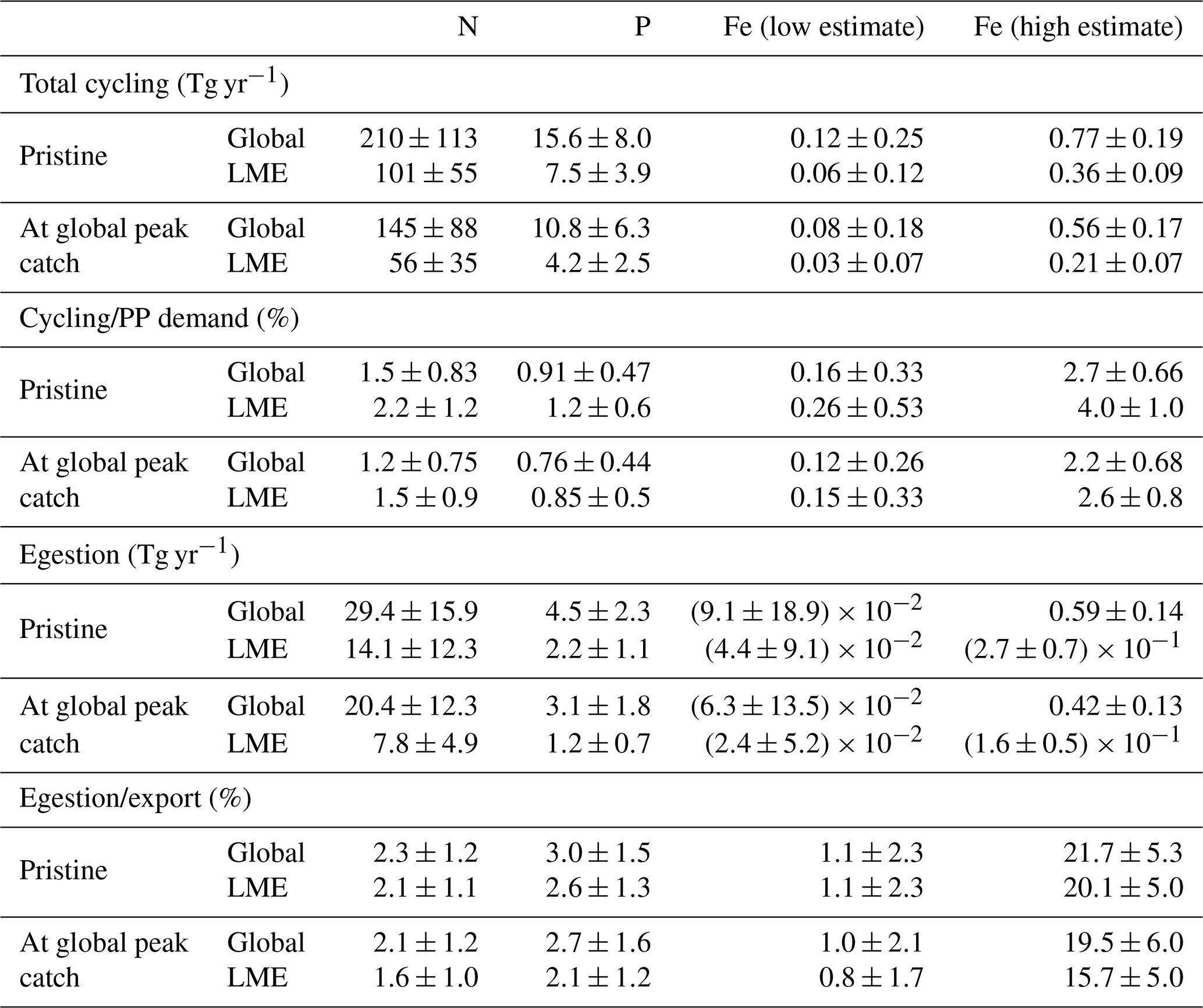
The global cycling, i.e., excretion plus egestion, of nutrients by the pristine biomass represents about 210±113 Tg N yr−1, 15.6±8.0 Tg P yr−1, and 0.12–0.77 Tg Fe yr−1, of which about half is in the LMEs (Table 3). Like nutrient storage, modeled cycling by fish is larger where the biomass is higher (Figs. 5 and S5). The three different ways of computing Fe cycling by the commercial fish biomass show similar spatial patterns, but Fe cycling is larger when using the weighted spatial variation between the low and high Fe : C estimates in zooplankton (Fig. 5). The spatially weighted computations suggest the possibility that Fe cycling by might be reduced in HNLC regions (principally in the Southern Ocean and the subarctic Pacific Ocean).
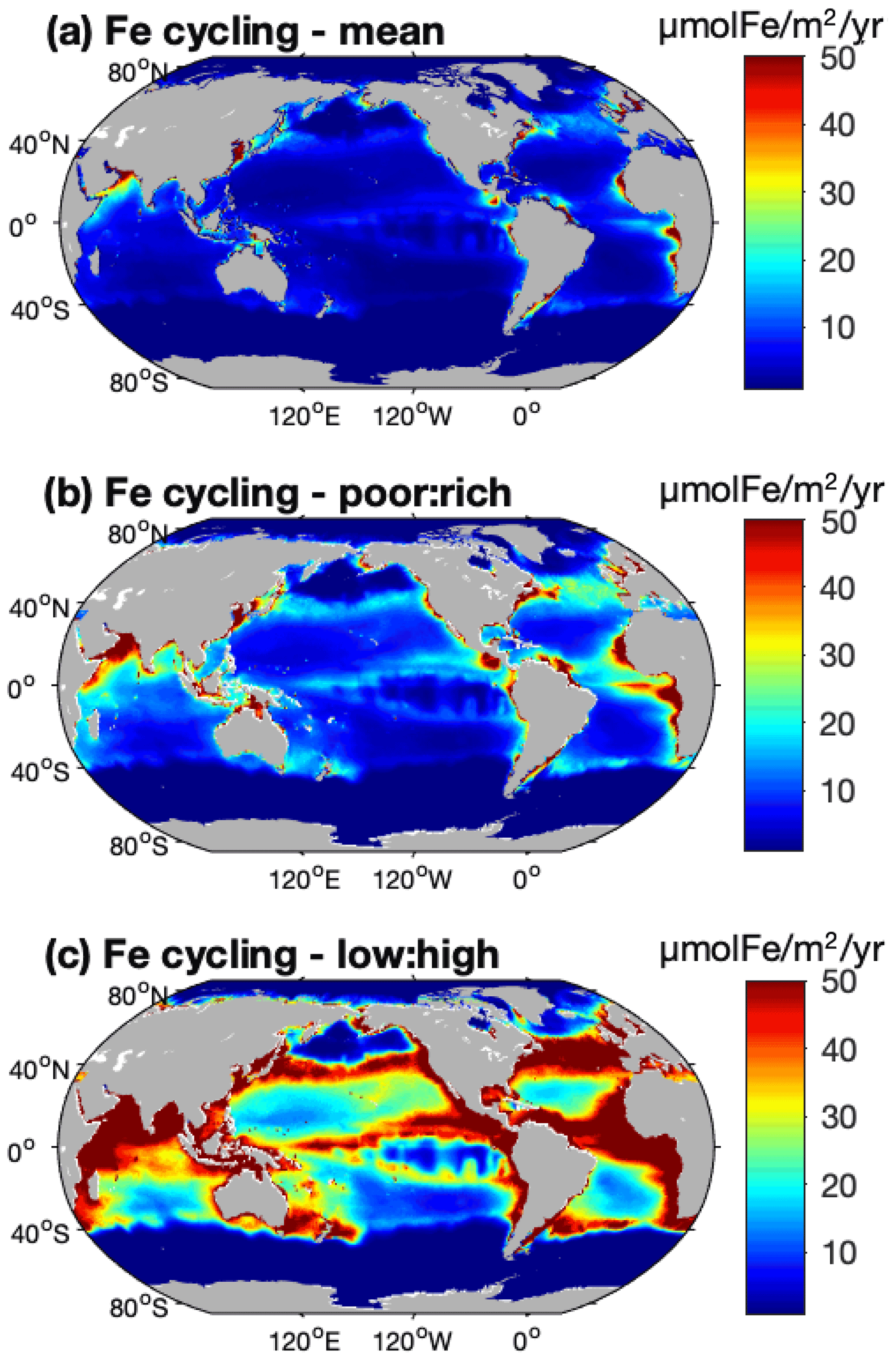
Figure 5Iron cycling by biomass computed using (a) a mean Fe : C in zooplankton, (b) a spatial variation between zooplankton Fe : C mean values in Fe-poor and Fe-rich areas and based on [NO3] concentrations, and (c) the same spatial variation but using the low and high estimates of zooplankton Fe : C from data. (For more details see Methods.)
4.1 Nutrient cycling by commercial fish relative to primary production
The modeled N cycling by pristine biomass contributes on average to 2.2±1.2 % of the N demand of primary producers (PP) in LMEs (Table 3) and generally accounts for less than 5 % of the demand, except in some coastal areas where it can be as high as 14 % (Fig. 6a). Similarly, the modeled pristine P cycling by represents 1.2 % of the total P demand in the LMEs (Table 3), less than 4 % of the global P demand with a larger contribution in the north and equatorial Atlantic coastal regions, and larger than 6 % contributions in some coastal areas (Fig. 6b). The high-end estimate of the Fe cycling by relative to PP demand for Fe is slightly more significant than the ratios for N and P, as it represents up to 13 % of the PP demand for Fe in some coastal areas and less than 10 % everywhere else (Fig. 6e).
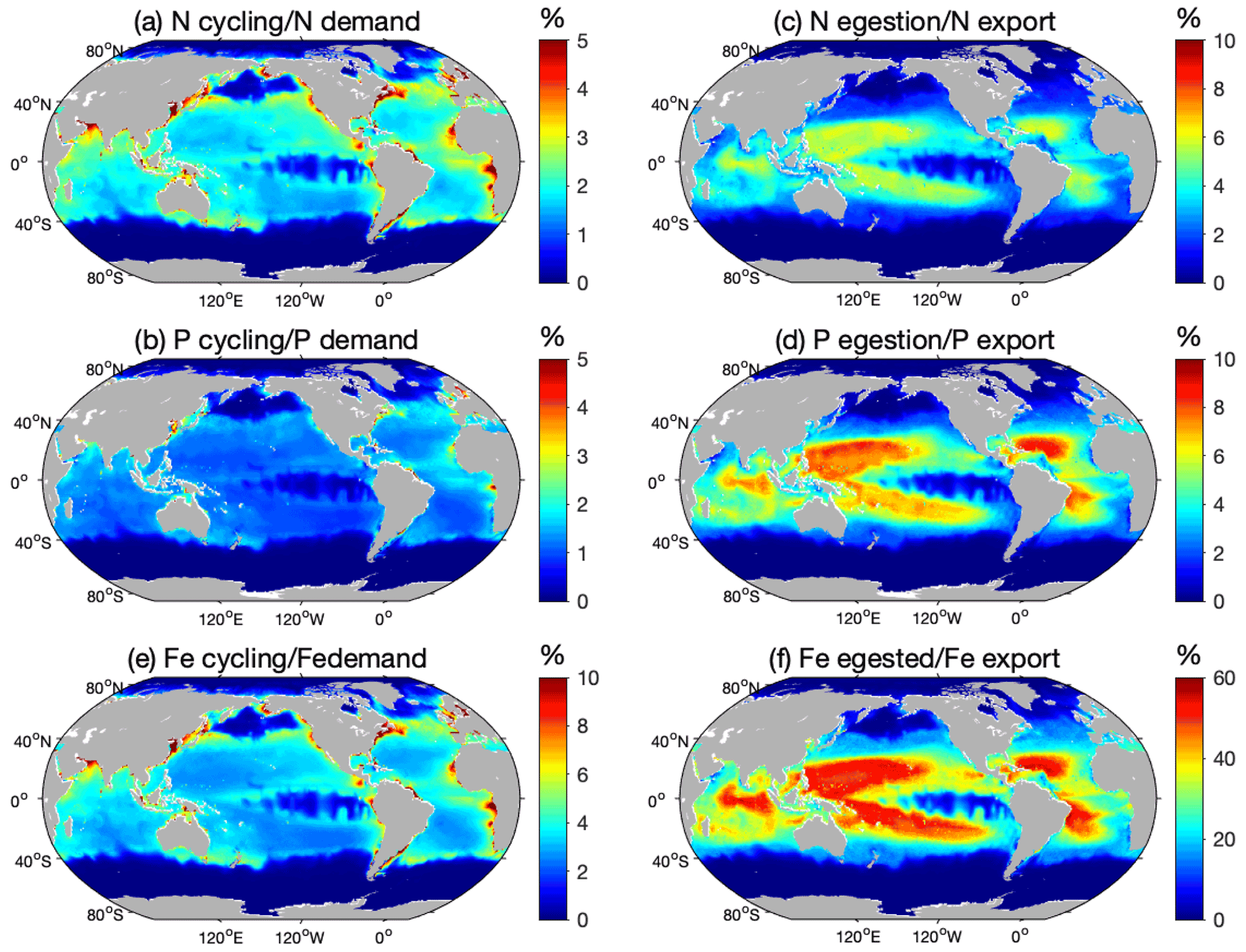
Figure 6Total nutrient cycling and egestion relative to export. Ratio (%) between the amount of nutrients cycled by the modeled pristine global biomass and estimated primary producers' demand for (a) N and (b) P, ratios of the modeled amount of nutrients egested by the pristine biomass and export at the base of the euphotic zone of (c) N and (d) P, and high-end estimate of the ratio (%) between the modeled amount of (e) Fe cycled by the modeled pristine global biomass and estimated primary producers' Fe demand, and (f) Fe egested by the pristine biomass and Fe export at the base of the euphotic zone. The high-end estimates are obtained using Fe cycling computed from the weighted spatial variation between the low and high Fe : C values of zooplankton and the weighted spatial variation between the averaged Fe : C ratios of phytoplankton in Fe-poor and Fe-rich conditions.
Our global estimates are broadly consistent with the order of magnitude influence of fish estimated by prior local studies. For all the coral reefs in the ocean, Allgeier et al. (2014) estimated that the total fish community supplies about 1.2 Tg N yr−1, which is about 0.6 % of our global pristine estimate (0.8 % compared to global cycling at peak catch) or 1.2 % of the LME pristine estimate (2.1 % of our N cycling by biomass at global peak catch) (Table 3)). This is consistent with the fact that coral reefs cover about 255 000–600 000 km2 (Spalding and Grenfell, 1997), which is about 0.4 %–0.8 % of the LME area. Hernández-León et al. (2008) estimated that zooplankton supply about 1780 Tg N yr−1 worldwide, representing 12 %–23 % of the requirements of phytoplankton and bacteria. This estimated zooplankton cycling is about 11 times our modeled recycling rate by the pristine biomass and 6–12 times what cycling could provide for primary producers. Given that the biomass distribution of all marine organisms has a slope of 0 (Hatton et al., 2021) (Fig. S7), and assuming that zooplankton mass ranges over 12 orders of magnitude, zooplankton biomass would be expected to be roughly 3 times the biomass of the total fish biomass in the 10 g to 100 kg size range. In addition, due to their higher metabolic and ingestion rates (Maldonado et al., 2016; Griffiths, 2006), zooplankton cycling rates are likely to be much higher than fish cycling rates, also exemplified by our modeled cycling size spectrum which has a negative slope (Fig. S8). McIntyre et al. (2008) showed that fish excretion can be important in supplying N and P to primary producers when conditions of high fish biomass and high PP demand or low ambient nutrient concentrations are combined and when nutrient inputs from anthropogenic sources are low. Our results indeed suggest an increased contribution of fish cycling when these conditions are combined. However, the strength of this contribution also depends on the timing between the release of nutrients by fish and the primary producers' demand for these nutrients.
For Fe, cycling represents a more important fraction of the PP demand compared to N and P, but large uncertainties remain in its computation. At the global scale, Moreno and Haffa (2014) estimated that the amount of Fe excreted by the commercial marine fish biomass ranged between 0.4–1.5 Tg Fe yr−1. Our modeled estimate range of 0.12–0.77 Tg Fe yr−1, based on the high and low estimates (Figs. 6e and S6), is lower but overlapping. The difference can in part be attributed to the lower Fe : C values we used for zooplankton (Table 1) and highlights the uncertainty on the Fe cycling computation (Fig. 5). In the Southern Ocean, whales have been shown to contribute to a maximum of 0.2 %–0.3 % of the phytoplankton demand for Fe in a pre-whaling ecosystem and no more than 0.03 %–0.04 % in a post-whaling ecosystem, making their contribution negligible compared to that of zooplankton (>70 % for microzooplankton only) (Maldonado et al., 2016). With a modeled contribution of about 0.05 %–0.5 % of the phytoplankton demand for Fe in the Southern Ocean, modeled pristine cycling coherently might be able to sustain a larger part of primary productivity than the current whale population but still far less than zooplankton as discussed before for N cycling.
Finally, fish movements also allow the transport of nutrients laterally in the ocean, constituting a sink of nutrients where the fish forage and a source of nutrients where the fish excrete, egest, or die (Vanni et al., 2013; Francis and Côté, 2018), an effect we do not explicitly include here.
4.2 Nutrient export by feces
Our results show that fish fecal material has the potential to affect the distribution of nutrients within the water column, especially in regions of low export intensity. Egested nutrients are integrated into fecal pellets that sink out of the surface layer and are recycled at greater depths than if bound to smaller particles (Wotton and Malmqvist, 2001; Turner, 2015), especially fish fecal pellets that can sink faster and deeper than marine snow and phytodetritus (Saba and Steinberg, 2012). Figure 6c–d, f quantify how much egestion may contribute to the export of N, P, and Fe to depth using the mean absorption efficiencies in Table 1 and assuming exported nutrient ratios, without fish, are on average equal to those of phytoplankton. For all the nutrients, -mediated export accounts for a larger part of the export in the warm, low-export regions of the world oceans, i.e., the tropical gyres, where it can contribute up to 50 % of the exported Fe for the high-end estimate (Fig. 6f), 6 % of the exported N, and 10 % of the exported P (Fig. 6c, d). Globally, modeled pristine biomass egests 29.4±15.9 Tg of N, 4.5±2.3 Tg of P, and 0.009–0.59 Tg of Fe each year, which on average roughly accounts for 2.3±1.2 %, 3.0±1.5 %, and 1.1 %–22 % of the export of N, P, and Fe, respectively, out of the euphotic zone (Table 3).
These results are in agreement with Davison et al. (2013), who showed that the contribution of mesopelagic fish to the carbon export (via respiration, excretion, egestion, and death) is higher in regions where the total export is small. However, Davison et al. (2013) also showed that locally, in the California Current, the active transport of C by mesopelagic fish alone, which we do not model, represents about 15 %–17 % of the total carbon export at depth. In their modeling study, Aumont et al. (2018) estimated that, globally, diurnal vertical migration of epipelagic organisms (all migrating fish and zooplankton) contributes to the flux of carbon to depth of about 18 % of the passive flux. Fish egesting and respiring at depth transport significant amounts of carbon and thus also transfer nutrients from the surface to deeper layers, a process that would have increased the contribution of fish to the export of nutrient if represented in the model.
More than the fish contribution to total export, their effect on particles may be most relevant for stoichiometric changes, especially for Fe. Indeed, since the absorption efficiency of Fe is smaller than that of C, the Fe : C in feces will be greater than in the ingested particles, and exported fecal material will have a greater Fe : C than biogenic sinking particles made of phytoplankton aggregates or dead organisms (Le Mézo and Galbraith, 2020). This is potentially important for mesopelagic organisms feeding on sinking material in light of the possible Fe limitation of marine animals (Le Mézo and Galbraith, 2020; Galbraith et al., 2019).
Until now we have considered as represented explicitly by the BOATS model, which ignores non-commercially targeted fish as well as the small and large ends of the fish size range. We provide a rough estimate of how the total fish biomass within a more inclusive marine size spectrum spanning 1g larvae to 106 g sharks () would compare to our estimates in two steps. First, we take the Bianchi et al. (2021) estimate that the is supported by roughly half of the total primary production that could be available to this size range (best estimate 58 %), from which we calculate that if the non-commercial fraction were included the total biomass estimate would be about 5.2 Gt. We then consider that the expanded size range includes 6 orders of magnitude compared to the 4 orders of magnitude of the standard BOATS size range. In BOATS, the size spectrum of abundance has a slope of about −1, giving the biomass size spectrum a slope of 0 (Fig. S7) consistent with the observed Sheldon spectrum (Hatton et al., 2021). Thus, by extension, we estimate that the biomass contains about 1.5 times (6 orders of magnitude versus 4 orders of magnitude) more biomass, giving a total of 7.8 Gt of wet biomass. Overall, we estimate that exceeds by a factor of 3.1.
The extended size spectrum contains more biomass, but it also contains more small fish than the standard size range of BOATS, a combination that would change the cycling rates of the total fish biomass. Since smaller fish are shown to have higher cycling rates than large ones (Clarke and Johnston, 1999), we expect higher cycling of nutrients by the extended size spectrum than would be implied by the larger biomass alone. In the pristine ocean modeled here by BOATS, the C cycling rates decrease with size following a slope of −0.37 mol C m−2 g−1 (Fig. S8). Based on this slope, and the biomass slope of 0, we would expect that the would have cycled about 2.4 times more C in the pristine ocean compared to the , with the 1–10 g size range cycling 40 % more C than the rest of the spectrum combined. Taken all together, the total cycling by would have been a factor of 4.8 greater than the rates discussed throughout the paper above. Assuming the additional organisms eat prey with similar body nutrient contents as the organisms already modeled, all of the nutrient cycling rates presented above would be increased proportionally.
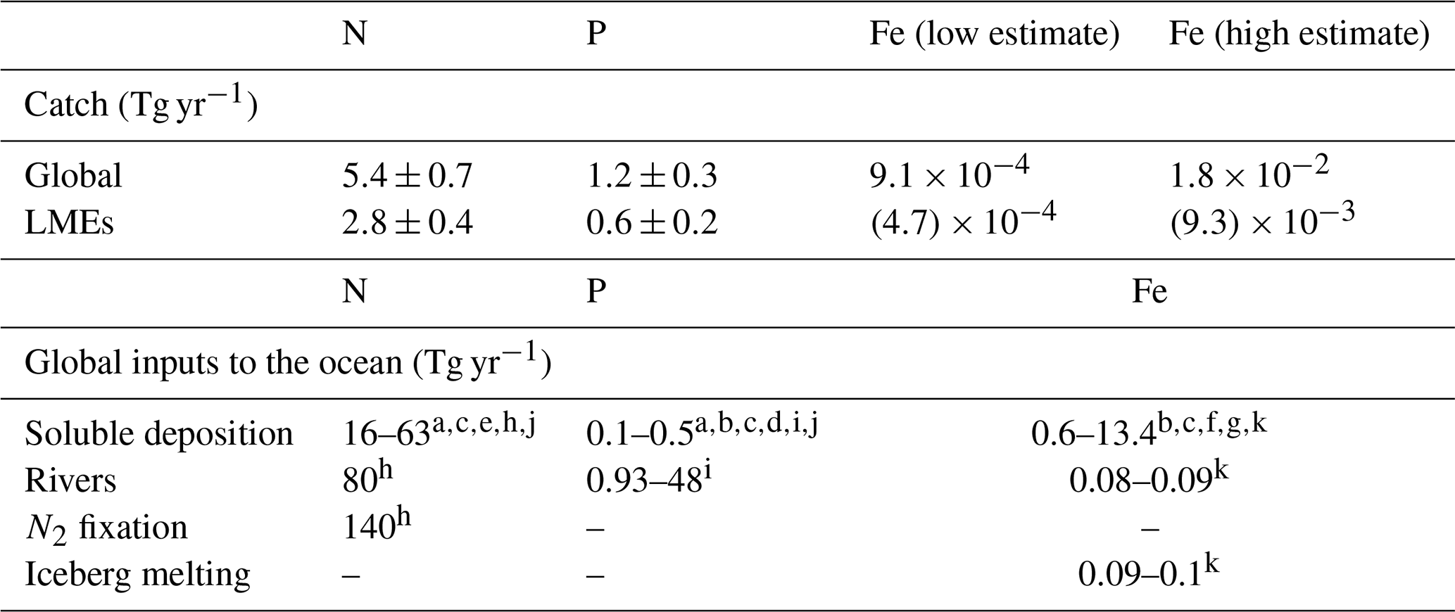
As fishing activity represents a direct removal of nutrients from the ocean, we estimated how much nutrients were extracted at the global peak catch and how these extraction rates would compare to nutrient inputs to the ocean. Globally, we estimate that modeled fishing activity removes 5.4±0.7 Tg N yr−1, 1.2±0.3 Tg P yr−1, and 0.09–1.8 × 10¹⁰ g Fe yr−1 from the ocean at the time of global peak catch, of which a little less than 50 % is in LMEs (Fig. 7, Table 4). Although our model is calibrated to agree reasonably well with observed catch maxima in LMEs over the years 1950 to 2010 (Pauly and Zeller, 2016; Bianchi et al., 2021), the total catch varies between ensemble members and tends to be overestimated in the open ocean, even with the Fe limitation we added in this study, for reasons that remain unclear. In addition, the catch estimate we present is at the time of the global peak catch in idealized simulations, rather than being historically accurate. Consequently, the simulated average catch at global peak (196.2±57 Tg wet weight) is higher than the peak catch estimated from fishery observations (130±65 Tg), so our estimates may exceed actual wild capture extractions by 50 %, with the most significant overestimates in the open ocean (see Bianchi et al., 2021, for more details).
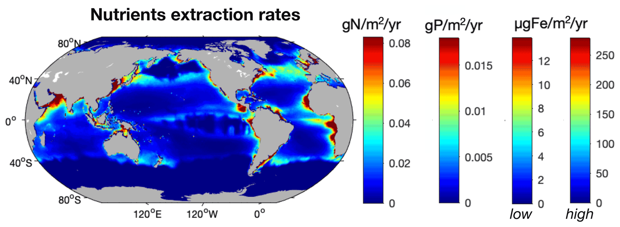
Figure 7Distribution of the modeled amount of N (g N m−2 yr−1), P (g P m−2 yr−1), and Fe ( µg Fe m−2 yr−1) extracted from the ocean at the time of the global peak catch. The two color bars for Fe represent the low and high estimates based on the 95 % confidence interval for Fe : C values in fish (10–200 µmol Fe (mol C)−1).
Table 4Table of values in LMEs from the model ensemble simulations in the pristine state and at the global peak catch. This table contains integrated values of the amount of nutrients removed by fishing in LMEs (Tg yr−1) and the ranges of values of the global nutrient inputs to the ocean from the literature (Tg yr−1).
a Brahney et al. (2015). b Mahowald et al. (2009). c Okin et al. (2011). d Myriokefalitakis et al. (2016). e Fowler et al. (2013). f Ito (2015). g Wang et al. (2015). h Gruber and Galloway (2008). i Benitez-Nelson (2000). j Kanakidou et al. (2012). k Moreno and Haffa (2014).
6.1 Nitrogen
Our estimate of N extraction from the catch is consistent with previous computations, and the differences mostly reflect the fish biomass estimates. For example, using catch data, Maranger et al. (2008) estimated the amount of N returned to land via fishing in LMEs to be about 0.9 Tg N yr−1 in the 1960s and 2.3 Tg N yr−1 in 2000. Our estimate of the N content of fish catch at global peak catch in LMEs is 2.8±0.4 Tg N yr−1, which is slightly larger than Maranger et al. (2008) estimate in 2000. Allgeier et al. (2017) also estimated the amount of N globally harvested to be about 2.072 Tg N yr−1 using the Maranger et al. (2008) 2.6 % N content and the FAO catch data. The FAO data only contain reported catches and consequently is lower than the SAUP data used in Maranger et al. (2008) and used to calibrate BOATS, which explains part of the difference.
Our study framework allows the spatial comparison of extracted nutrients to nutrient inputs, which was not the case in previous work. For N, even though N extraction by fishing can be significant locally compared to N deposition at the surface, N extraction is negligible compared to the other sources of N to the surface layers. Figure 8a compares the amount of N extracted by fishing to the modeled soluble atmospheric N deposition from Brahney et al. (2015). Globally, fishing removal of N is smaller than current modeled atmospheric deposition of soluble N, with the higher values, up to more than 60 % of the N deposition, in the southern equatorial Pacific, along the western margins of Africa and South America, and in the Arabian Sea, where catch is high and deposition is low (Fig. S3). However, most of N supply to the surface ocean occurs through vertical diffusion and mixing of the upper layers (Sarmiento and Gruber, 2006), which likely accentuates the fact that N extraction by fishing is insignificant at the global scale.

Figure 8Ratio (%) between simulated extracted nutrients and current aeolian soluble nutrient inputs at the surface of the ocean for (a) N and (b) Fe. “low” and “high” refer to the use of 10 or 200 µmol Fe (mol C)−1 in fish, respectively.
6.2 Phosphorus
Similarly to N, our estimate of P extraction by fishing is coherent with previous work and shows that it is very small compared to inputs of P to the ocean and resupply from vertical mixing and diffusion in the water column. We estimate that the amount of P removed by fishing at the global scale amounts to 1.2±0.3 Tg P yr−1, of which 0.6±0.2 Tg P yr−1 occurs in the LMEs (Table 4). Huang et al. (2020) estimated that wild and aquaculture fisheries, including finfish, crustaceans, and molluscs, represented 1.1 Tg of P in 2016, which is superficially similar to our estimate. However, our estimated catch of 196.2±57 Tg of wet weight is larger than the global amount of catch they used of 169 Tg, even though they considered aquaculture in addition to wild captures. Our catch estimate at global peak catch overestimates the high seas catch as discussed at the beginning of this section and in Bianchi et al. (2021). Additionally, our estimate is solely based on fish P content (Table 1), which may slightly overestimate the amount of P extracted by fishing activity since crustaceans and molluscs have lower P content than finfish (Huang et al., 2020).
Contrary to N, the modeled removal of P from harvest would largely exceed the atmospheric deposition of soluble P as P inputs to the ocean mostly occur through riverine inputs (Table 4). Consequently, catch transfers P from the ocean to land whereas P supply to the ocean is mostly occurring in the coastal areas, with possible impacts on the P budget of the open ocean (Huang et al., 2020). But similarly to N, vertical diffusion and mixing of the upper layers supply P to the surface ocean in quantities that most likely render P extraction by fishing relatively insignificant.
6.3 Iron
Fe extraction by fishing activity is within the range of previous estimates, but large uncertainties remain due to uncertainty regarding the Fe : C of fish. Moreno and Haffa (2014) investigated the extent to which commercial catch has globally translocated Fe from the ocean to land. They estimated the global rate of translocation of Fe to be between 0.007 and 0.03 Tg in 2010. Our modeled global range of Fe removal is about 0.0009–0.018 Tg Fe yr−1 (Fig. 7, Table 4). Our lower estimated values can once again be explained by the difference in the Fe : C ratios used for fish. Even though our estimate is lower, it shows that locally Fe extraction can be significant compared to Fe inputs from dust deposition. Although the high-end estimate of Fe extracted is globally small relative to modeled soluble Fe deposition from Mahowald et al. (2009), it reaches values larger than 100 % in the coastal eastern equatorial Pacific and in some other coastal areas such as western South Africa, northern Europe, and Canada (Fig. 8b), where modeled Fe deposition is small and harvest is high (Fig. S3). Contrary to N and P, Fe has a much shorter residence time and thus is subject to local perturbations, among which Fe extraction by fishing could be important.
6.4 Local and time-dependent nutrient budgets
Nutrient budgets are subject to perturbations in space and in time that can modify the relative strength of the nutrient extraction by fishing activity. Some local nutrient budgets have been investigated to compare the amount of nutrients extracted by fishing to the nutrient loads (e.g., Hjerne and Hansson, 2002). If we were to do similar budgets, at the global scale, assuming all P inputs come from rivers and atmospheric deposition, which represents 48.5 Tg P yr−1 (Tables 4 and S1), then the extracted P flux represents 2.5 % of the global input flux (1.2 % over the LMEs). For N, global catch represents about 2 % of the combined N inputs from atmospheric deposition (49.6 Tg N yr−1), rivers (80 Tg N yr−1), and N2 fixation (140 Tg N yr−1) (Tables 4 and S1).
Note that fish extracted from a given area may have foraged elsewhere, especially large fish able to undertake long-distance migrations like tuna, salmon, or sharks (e.g., Afonso et al., 2017; Gresh et al., 2000). Consequently, the ratios between extracted nutrients and nutrient deposition may be over- or under-estimated, thus over- or under-estimating the role of fishing as a local sink of nutrients (Vanni et al., 2013). In addition, the relative timing of fishing effort along with phytoplankton growth, nutrient input seasonality, and residence times may also modify the importance of fishing activity as a sink of nutrients (e.g., Francis and Côté, 2018; Vanni et al., 2006).
6.5 Reductions in nutrient cycling caused by fishing
Fishing has had a dramatic influence on nutrient cycling by , as it has permanently removed a large amount of biomass, especially in the large size classes. In our ensemble of simulations, the cycling rates decrease by about 30 % for the three elements considered at the time of the global peak catch (Table 3), due to the global reduction in fish biomass of about 60 %. Since large fish are heavily targeted by fisheries, the size spectrum of CTF appears truncated at a larger size class at the time of the global peak catch compared to a pristine state (Fig. S7). This reduction of the mean community size enhances the cycling of elements as smaller animals tend to have higher metabolic rates (e.g., Schmitz et al., 2010; Vanni, 2002), so that the reduction in overall cycling rate is roughly half the reduction of biomass.
Finally, as the size classes below 10 g are not resolved (Fig. 2), we are not able to account for biomass changes that fishing might induce through trophic cascades, or how it reverberates up to fish through food supply (Dupont et al., 2022), which has the potential to further modify fish-mediated nutrient cycling.
In this study, we estimate the amount of N, P, and Fe contained in and cycled by the global biomass, both in its pristine state and at the time of the global peak catch. The overall contribution of this commercial ichthyosphere to oceanic nutrient cycling is relatively small but is more significant in regions of low ambient nutrient concentrations, high fish biomass, and low export production. The industrial fish catch generally represents a small extraction of nutrients globally compared to external inputs, though it removes a significant amount of P from the open ocean compared to external inputs (mainly riverine). In general, local cycling of N and P by fish is less significant than Fe cycling by fish because N and P are resupplied globally through large-scale circulation processes, while Fe cycling is more local and susceptible to perturbations through rapid scavenging for example. In addition, poor absorption of Fe by fish leads to an enrichment of the Fe content of fecal matter.
Globally, nutrient cycling by the modeled biomass is small compared to primary producers' demand for these nutrients. The highest contributions are found close to the coasts where fish biomass and productivity demand are high. Fish egestion of nutrients via faecal pellets is likely to comprise the largest fraction of the sinking flux in regions of low export production, i.e., the subtropical gyres. Fecal pellets may also significantly impact the stoichiometry of sinking particles, especially for Fe, with consequences for mesopelagic organisms.
Our study provides a first global glimpse of nutrient cycling by the ichthyosphere. Although the contribution of simulated by our model tends to be on the order of only a few percent of total surface nutrient budgets and fluxes, we estimate that these would be a factor of 3 or more larger for the 1 g to 1000 kg range, including all fish. Furthermore, the role of fish in shaping the ecosystem processes through top-down pressure on their prey may be of similar or greater magnitude than the quantities estimated here (Frank et al., 2005; Baum and Worm, 2009; Hessen and Kaartvedt, 2014; Kavanagh and Galbraith, 2018). Fish can also be highly relevant at the local scale, for example by changing the vertical distribution of Fe in the water column as mentioned above, and as highlighted by many studies on fish in coral reefs. Unresolved factors, such as fish migrations, would alter our results and the sensitivity of fish-mediated nutrient cycling to warming and deoxygenation due to climate change (e.g., Lefort et al., 2015; Lotze et al., 2019). There remains much to be learned about the role of fish in global nutrient cycling.
Model outputs and code used to analyze them can be found here: https://doi.org/10.5281/zenodo.6538917 (Le Mézo et al., 2022).
The supplement related to this article is available online at: https://doi.org/10.5194/bg-19-2537-2022-supplement.
PLM, EG, and DB designed the study. KS provided the updated model version. JG performed the simulations and the model–data comparison. PLM made the figures and wrote the manuscript. All the authors revised the manuscript.
The contact author has declared that neither they nor their co-authors have any competing interests.
Publisher’s note: Copernicus Publications remains neutral with regard to jurisdictional claims in published maps and institutional affiliations.
We thank the reviewers and the editor for their very helpful comments on the manuscript and all the members of the BIGSEA group for the multiple exchanges on the subject.
This research has been supported by the European Research Council (ERC) under the European Union’s Horizon 2020 research and innovation programme (BIGSEA, grant no. 682602), the California Ocean Protection Council (grant no. C0100400), NASA (grant no. 80NSSC21K0420), the French ANR project CIGOEF (grant no. ANR-17-CE32-0008-01), and the Extreme Science and Engineering Discovery Environment (XSEDE, grant no. TG-OCE170017).
This paper was edited by Kenneth Rose and reviewed by Jacob Allgeier and Emma Cavan.
Afonso, A. S., Garla, R., and Hazin, F. H. V.: Tiger sharks can connect equatorial habitats and fisheries across the Atlantic Ocean basin, PLOS ONE, 12, e0184763, https://doi.org/10.1371/journal.pone.0184763, 2017. a
Allgeier, J. E., Layman, C. A., Mumby, P. J., and Rosemond, A. D.: Consistent nutrient storage and supply mediated by diverse fish communities in coral reef ecosystems, Glob. Change Biol., 20, 2459–2472, https://doi.org/10.1111/gcb.12566, 2014. a, b, c
Allgeier, J. E., Valdivia, A., Cox, C., and Layman, C. A.: Fishing down nutrients on coral reefs, Nat. Commun., 7, 1–5, https://doi.org/10.1038/ncomms12461, 2016. a, b, c
Allgeier, J. E., Burkepile, D. E., and Layman, C. A.: Animal pee in the sea: consumer-mediated nutrient dynamics in the world's changing oceans, Glob. Change Biol., 23, 2166–2178, https://doi.org/10.1111/gcb.13625, 2017. a, b, c, d, e
Allgeier, J. E., Wenger, S., and Layman, C. A.: Taxonomic identity best explains variation in body nutrient stoichiometry in a diverse marine animal community, Sci. Rep., 10, 1–10, https://doi.org/10.1038/s41598-020-67881-y, 2020. a, b
Aqua MODIS: NASA goddard space flight center, ocean ecology laboratory, ocean biology processing group, Moderate-resolution Imaging Spectroradiometer (MODIS) Aqua Euphotic Depth Data; 2018 Reprocessing, NASA OB, DAAC, Greenbelt, MD, USA, https://doi.org/10.5067/AQUA/MODIS/L3M/ZLEE/2018, 2018. a, b
Atkinson, C. L., Capps, K. A., Rugenski, A. T., and Vanni, M. J.: Consumer-driven nutrient dynamics in freshwater ecosystems: from individuals to ecosystems, Biol. Rev., 92, 2003–2023, https://doi.org/10.1111/brv.12318, 2017. a
Aumont, O., Maury, O., Lefort, S., and Bopp, L.: Evaluating the Potential Impacts of the Diurnal Vertical Migration by Marine Organisms on Marine Biogeochemistry, Global Biogeochem. Cy., 32, 1622–1643, https://doi.org/10.1029/2018GB005886, 2018. a
Baum, J. K. and Worm, B.: Cascading top-down effects of changing oceanic predator abundances, J. Anim. Ecol., 78, 699–714, https://doi.org/10.1111/j.1365-2656.2009.01531.x, 2009. a
Benitez-Nelson, C. R.: The biogeochemical cycling of phosphorus in marine systems, Earth Sci. Rev., 51, 109–135, https://doi.org/10.1016/S0012-8252(00)00018-0, 2000. a
Bianchi, D., Galbraith, E. D., Carozza, D. A., Mislan, K. A. S., and Stock, C. A.: Intensification of open-ocean oxygen depletion by vertically migrating animals, Nat. Geosci., 6, 1–5, https://doi.org/10.1038/ngeo1837, 2013. a
Bianchi, D., Carozza, D. A., Galbraith, E. D., Guiet, J., and DeVries, T.: Estimating global biomass and biogeochemical cycling of marine fish with and without fishing, Sci. Adv., 7, 41, https://doi.org/10.1126/sciadv.abd7554, 2021. a, b, c, d, e, f, g, h, i, j, k, l, m
Brahney, J., Mahowald, N., Ward, D. S., Ballantyne, A. P., and Neff, J. C.: Is atmospheric phosphorus pollution altering global alpine Lake stoichiometry?, Global Biogeochem. Cy., 29, 1369–1383, https://doi.org/10.1002/2015GB005137, 2015. a, b, c
Carozza, D. A., Bianchi, D., and Galbraith, E. D.: The ecological module of BOATS-1.0: a bioenergetically constrained model of marine upper trophic levels suitable for studies of fisheries and ocean biogeochemistry, Geosci. Model Dev., 9, 1545–1565, https://doi.org/10.5194/gmd-9-1545-2016, 2016. a, b, c, d
Carozza, D. A., Bianchi, D., and Galbraith, E. D.: Formulation, General Features and Global Calibration of a Bioenergetically-Constrained Fishery Model, PLOS ONE, 12, e0169763, https://doi.org/10.1371/journal.pone.0169763, 2017. a, b, c, d
Cavan, E. L., Belcher, A., Atkinson, A., Hill, S. L., Kawaguchi, S., McCormack, S., Meyer, B., Nicol, S., Ratnarajah, L., Schmidt, K., Steinberg, D. K., Tarling, G. A., and Boyd, P. W.: The importance of Antarctic krill in biogeochemical cycles, Nat. Commun., 10, 1–13, https://doi.org/10.1038/s41467-019-12668-7, 2019. a
Chassot, E., Bonhommeau, S., Dulvy, N. K., Mélin, F., Watson, R., Gascuel, D., and Le Pape, O.: Global marine primary production constrains fisheries catches, Ecol. Lett., 13, 495–505, 2010. a
Clarke, A. and Johnston, N. M.: Scaling of metabolic rate with body mass and temperature in teleost fish, J. Anim. Ecol., 68, 893–905, 1999. a
Czamanski, M., Nugraha, A., Pondaven, P., Lasbleiz, M., Masson, A., Caroff, N., Bellail, R., and Tréguer, P.: Carbon, nitrogen and phosphorus elemental stoichiometry in aquacultured and wild-caught fish and consequences for pelagic nutrient dynamics, Mar. Biol., 158, 2847–2862, https://doi.org/10.1007/s00227-011-1783-7, 2011. a, b, c
Davison, P. C., Checkley, D. M., Koslow, J. A., and Barlow, J.: Carbon export mediated by mesopelagic fishes in the northeast Pacific Ocean, Prog. Oceanogr., 116, 14–30, https://doi.org/10.1016/j.pocean.2013.05.013, 2013. a, b, c
Dunne, J. P., Sarmiento, J. L., and Gnanadesikan, A.: A synthesis of global particle export from the surface ocean and cycling through the ocean interior and on the seafloor, Global Biogeochem. Cy., 21, GB4006, https://doi.org/10.1029/2006GB002907, 2007. a, b, c
Dunne, J. P., John, J. G., Shevliakova, S., Stouffer, R. J., Krasting, J. P., Malyshev, S. L., Milly, P. C., Sentman, L. T., Adcroft, A. J., Cooke, W., Dunne, K. A., Griffies, S. M., Hallberg, R. W., Harrison, M. J., Levy, H., Wittenberg, A. T., Phillips, P. J., and Zadeh, N.: GFDL's ESM2 global coupled climate-carbon earth system models. Part II: Carbon system formulation and baseline simulation characteristics, J. Climate, 26, 2247–2267, https://doi.org/10.1175/JCLI-D-12-00150.1, 2013. a, b
Dupont, L., Le Mézo, P., Clerc, C., Maury, O., Aumont, O., Ethé, C., and Bopp, L.: High trophic level feedbacks on ocean biogeochemistry under climate change, submitted, 2022. a
El-Sabaawi, R. W., Warbanski, M. L., Rudman, S. M., Hovel, R., and Matthews, B.: Investment in boney defensive traits alters organismal stoichiometry and excretion in fish, Oecologia, 181, 1209–1220, https://doi.org/10.1007/s00442-016-3599-0, 2016. a
Fowler, D., Coyle, M., Skiba, U., Sutton, M., Cape, J. N., Reis, S., Sheppard, L., Jenkins, A., Grizetti, B., Galloway, J. N., Vitousek, P., Leach, A., Bouwman, L., Butterbach-Bahl, K., Dentener, F., Stevenson, D., Amann, M., and Voss, M.: The global nitrogen cycle in the 21th century, Philis. T. R. Soc. Lon. B, 368, 1621, https://doi.org/10.1098/rstb.2013.0164, 2013. a
Francis, F. T. and Côté, I. M.: Fish movement drives spatial and temporal patterns of nutrient provisioning on coral reef patches, Ecosphere, 9, e02225, https://doi.org/10.1002/ecs2.2225, 2018. a, b, c
Frank, K. T., Petrie, B., Choi, J. S., and Leggett, W. C.: Trophic cascades in a formerly cod-dominated ecosystem., Science, 308, 1621–1623, https://doi.org/10.1126/science.1113075, 2005. a
Galbraith, E. D. and Martiny, A. C.: A simple nutrient-dependence mechanism for predicting the stoichiometry of marine ecosystems, P. Natl. Acad. Sci. USA, 112, 8199–8204, https://doi.org/10.1073/pnas.1423917112, 2015. a, b
Galbraith, E. D., Carozza, D. A., and Bianchi, D.: A coupled human-Earth model perspective on long-term trends in the global marine fishery, Nat. Commun., 8, 1–7, https://doi.org/10.1038/ncomms14884, 2017. a, b
Galbraith, E. D., Le Mézo, P. K., Solanes Hernandez, G., Bianchi, D., and Kroodsma, D.: Growth limitation of marine fish by low iron availability in the open ocean, Frontiers in Marine Science, 6, 1–13, https://doi.org/10.3389/fmars.2019.00509, 2019. a, b, c, d, e, f, g, h, i, j
Garcia, H. E., Locarnini, R. A., Boyer, T. P., Antonov, J. I., Baranova, O. K., Zweng, M. M., Reagan, J. R., Johnson, D. R., Mishonov, A. V., and Levitus, S.: World ocean atlas 2013, Volume 4, Dissolved inorganic nutrients (phosphate, nitrate, silicate), NOAA institutional repository, NOAA atlas NESDIS, 76, https://doi.org/10.7289/V5J67DWD, 2013. a
Gordon, H. S.: The Economic Theory of a Common-Property Resource: The Fishery, Education + Training, 62, 124–142, 1954. a
Gresh, T., Lichatowich, J., and Schoonmaker, P.: An Estimation of Historic and Current Levels of Salmon Production in the Northeast Pacific Ecosystem: Evidence of a Nutrient Deficit in the Freshwater Systems of the Pacific Northwest, Fisheries, 25, 15–21, https://doi.org/10.1577/1548-8446(2000)025<0015:AEOHAC>2.0.CO;2, 2000. a
Griffiths, D.: The direct contribution of fish to lake phosphorus cycles, Ecol. Freshw. Fish, 15, 86–95, https://doi.org/10.1111/j.1600-0633.2006.00125.x, 2006. a, b, c
Gruber, N. and Galloway, J. N.: An Earth-system perspective of the global nitrogen cycle, Nature, 451, 293–296, https://doi.org/10.1038/nature06592, 2008. a
Guiet, J., Galbraith, E., Bianchi, D., and Cheung, W.: Bioenergetic influence on the historical development and decline of industrial fisheries, ICES J. Mar. Sci., 77, 1854–1863, 2020. a
Hall, R. O. J., Koch, B. J., Marshall, M. C., Taylor, B. W., How, L. M. T., Koch, B. J., Marshall, M. C., and Taylor, B. W.: How body size mediates the role of animals in nutrient cycling in aquatic ecosystems, The structure and function of aquatic ecosystems, Cambridge University Press New York, NY, 286–305, https://doi.org/10.1017/CBO9780511611223, 2007. a
Halvorson, H. M. and Small, G. E.: Observational field studies are not appropriate tests of consumer stoichiometric homeostasis, Freshw. Sci., 35, 1103–1116, https://doi.org/10.1086/689212, 2016. a, b
Hatton, I. A., Heneghan, R. F., Bar-On, Y. M., and Galbraith, E. D.: The global ocean size spectrum from bacteria to whales, Sci. Adv., 7, 1–9, https://doi.org/10.1126/sciadv.abh3732, 2021. a, b, c
Hernández-León, S., Fraga, C., and Ikeda, T.: A global estimation of mesozooplankton ammonium excretion in the open ocean, J. Plankton Res., 30, 577–585, https://doi.org/10.1093/plankt/fbn021, 2008. a
Hessen, D. O. and Kaartvedt, S.: Top-down cascades in lakes and oceans: Different perspectives but same story?, J. Plankton Res., 36, 914–924, https://doi.org/10.1093/plankt/fbu040, 2014. a
Hicks, C. C., Cohen, P. J., Graham, N. A. J., Nash, K. L., Allison, E. H., D'Lima, C., Mills, D. J., Roscher, M., Thilsted, S. H., Thorne-Lyman, A. L., and MacNeil, M. A.: Harnessing global fisheries to tackle micronutrient deficiencies, Nature, 574, 95–98, https://doi.org/10.1038/s41586-019-1592-6, 2019. a
Hjerne, O. and Hansson, S.: The role fish and fisheries in the Baltic sea nutrient dyanmics, Limnol. Oceanogr., 47, 1023–1032, 2002. a, b, c
Huang, Y., Ciais, P., Goll, D. S., Sardans, J., Peñuelas, J., Cresto-Aleina, F., and Zhang, H.: The shift of phosphorus transfers in global fisheries and aquaculture, Nat. Commun., 11, 1–10, https://doi.org/10.1038/s41467-019-14242-7, 2020. a, b, c
Ito, A.: Atmospheric Processing of Combustion Aerosols as a Source of Bioavailable Iron, Environ. Sci. Technol. Lett., 2, 70–75, https://doi.org/10.1021/acs.estlett.5b00007, 2015. a
Jennings, S., Mélin, F., Blanchard, J. L., Forster, R. M., Dulvy, N. K., Wilson, R. W., Jennings, S., Dulvy, N. K., Wilson, R. W., Melin, F., Blanchard, J. L., Forster, R. M., Dulvy, N. K., Wilson, R. W., Mélin, F., Blanchard, J. L., Forster, R. M., Dulvy, N. K., and Wilson, R. W.: Global-scale predictions of community and ecosystem properties from simple ecological theory, P. Roy. Soc. B, 275, 1375–1383, https://doi.org/10.1098/rspb.2008.0192, 2008. a, b
Kanakidou, M., Duce, R. A., Prospero, J. M., Baker, A. R., Benitez-Nelson, C., Dentener, F. J., Hunter, K. A., Liss, P. S., Mahowald, N., Okin, G. S., Sarin, M., Tsigaridis, K., Uematsu, M., Zamora, L. M., and Zhu, T.: Atmospheric fluxes of organic N and P to the global ocean, Global Biogeochem. Cy., 26, 1–12, https://doi.org/10.1029/2011GB004277, 2012. a
Kavanagh, L. and Galbraith, E.: Links between fish abundance and ocean biogeochemistry as recorded in marine sediments, PLoS ONE, 13, 1–22, https://doi.org/10.1371/journal.pone.0199420, 2018. a
Layman, C. A., Allgeier, J. E., Rosemond, A. D., Dahlgren, C. P., and Yeager, L. A.: Marine fisheries declines viewed upside down: Human impacts on consumer-driven nutrient recycling, Ecol. Appl., 21, 343–349, https://doi.org/10.1890/10-1339.1, 2011. a, b
Lefort, S., Aumont, O., Bopp, L., Arsouze, T., Gehlen, M., and Maury, O.: Spatial and body-size dependent response of marine pelagic communities to projected global climate change, Glob. Change Biol., 21, 154–164, https://doi.org/10.1111/gcb.12679, 2015. a
Le Mézo, P. K. and Galbraith, E. D.: The fecal iron pump : impact of animals on the Fe stoichiometry of marine sinking particles, Limnol. Oceanogr., 66, 1–39, 2020. a, b, c
Le Mézo, P., Guiet, J., Scherrer, K., Bianchi, D., and Galbraith, E.: Global nutrient cycling by commercially targeted marine fish (Le Mézo et al., 2022, Biogeosciences), Zenodo [data set], https://doi.org/10.5281/zenodo.6538917, 2022. a
Leroux, S. J. and Schmitz, O. J.: Predator-driven elemental cycling: the impact of predation and risk effects on ecosystem stoichiometry, Ecol. Evol., 5, 4976–4988, https://doi.org/10.1002/ece3.1760, 2015. a
Lotze, H. K., Tittensor, D. P., Bryndum-Buchholz, A., Eddy, T. D., Cheung, W. W., Galbraith, E. D., Barange, M., Barrier, N., Bianchi, D., Blanchard, J. L., Bopp, L., Büchner, M., Bulman, C. M., Carozza, D. A., Christensen, V., Coll, M., Dunne, J. P., Fulton, E. A., Jennings, S., Jones, M. C., Mackinson, S., Maury, O., Niiranen, S., Oliveros-Ramos, R., Roy, T., Fernandes, J. A., Schewe, J., Shin, Y. J., Silva, T. A., Steenbeek, J., Stock, C. A., Verley, P., Volkholz, J., Walker, N. D., and Worm, B.: Global ensemble projections reveal trophic amplification of ocean biomass declines with climate change, P. Natl. Acad. Sci. USA, 116, 12907–12912, https://doi.org/10.1073/pnas.1900194116, 2019. a
Mahowald, N. M., Engelstaedter, S., Luo, C., Sealy, A., Artaxo, P., Benitez-Nelson, C., Bonnet, S., Chen, Y., Chuang, P. Y., Cohen, D. D., Dulac, F., Herut, B., Johansen, A. M., Kubilay, N., Losno, R., Maenhaut, W., Paytan, A., Prospero, J. M., Shank, L. M., and Siefert, R. L.: Atmospheric Iron Deposition: Global Distribution, Variability, and Human Perturbations, Annu. Rev. Mar. Sci., 1, 245–278, https://doi.org/10.1146/annurev.marine.010908.163727, 2009. a, b, c, d
Maldonado, M. T., Surma, S., and Pakhomov, E. A.: Southern Ocean biological iron cycling in the pre-whaling and present ecosystems, Philos. T Roy Soc A, 374, 2081, https://doi.org/10.1098/rsta.2015.0292, 2016. a, b
Maranger, R., Caraco, N., Duhamel, J., and Amyot, M.: Nitrogen transfer from sea to land via commercial fisheries, Nat. Geosci., 1, 111–113, https://doi.org/10.1038/ngeo108, 2008. a, b, c, d, e, f
McIntyre, P. B., Flecker, A. S., Vanni, M. J., Hood, J. M., Taylor, B. W., and Thomas, S. A.: Fish distributions and nutrient recycling in streams: can fish create biogeochemical hotspots?, Ecology, 89, 2335–2346, 2008. a, b
Moore, C. M., Mills, M. M., Arrigo, K. R., Berman-Frank, I., Bopp, L., Boyd, P. W., Galbraith, E. D., Geider, R. J., Guieu, C., Jaccard, S. L., Jickells, T. D., La Roche, J., Lenton, T. M., Mahowald, N. M., Marañón, E., Marinov, I., Moore, J. K., Nakatsuka, T., Oschlies, A., Saito, M. A., Thingstad, T. F., Tsuda, A., and Ulloa, O.: Processes and patterns of oceanic nutrient limitation, Nat. Geosci., 6, 701–710, https://doi.org/10.1038/ngeo1765, 2013. a, b
Moreno, A. R. and Haffa, A. L. M.: The Impact of Fish and the Commercial Marine Harvest on the Ocean Iron Cycle, PLoS ONE, 9, e107690, https://doi.org/10.1371/journal.pone.0107690, 2014. a, b, c, d, e, f
Myriokefalitakis, S., Nenes, A., Baker, A. R., Mihalopoulos, N., and Kanakidou, M.: Bioavailable atmospheric phosphorous supply to the global ocean: a 3-D global modeling study, Biogeosciences, 13, 6519–6543, https://doi.org/10.5194/bg-13-6519-2016, 2016. a, b
Okin, G. S., Baker, A. R., Tegen, I., Mahowald, N. M., Dentener, F. J., Duce, R. A., Galloway, J. N., Hunter, K., Kanakidou, M., Kubilay, N., Prospero, J. M., Sarin, M., Surapipith, V., Uematsu, M., and Zhu, T.: Impacts of atmospheric nutrient deposition on marine productivity: Roles of nitrogen, phosphorus, and iron, Global Biogeochem. Cy., 25, 1–10, https://doi.org/10.1029/2010GB003858, 2011. a
Pauly, D. and Tsukayama, I.: On the seasonal growth, monthly recruitment and monthly biomass of Peruvian anchoveta (Engraulis ringens) from 1961 to 1979, in: Proceedings of the expert consultation to examine changes in abundance and species composition of neritic fish resources, San José, Costa Rica, 18–29 April 1983, FAO fishery report 291, edited by: Sharp, G. D. and Csirke, J., vol. 3, 987–1004, 1984. a
Pauly, D. and Zeller, D.: Catch reconstructions reveal that global marine fisheries catches are higher than reported and declining, Nat. Commun., 7, 10244, https://doi.org/10.1038/ncomms10244, 2016. a, b
Pilati, A. and Vanni, M. J.: Ontogeny, diet shifts, and nutrient stoichiometry in fish, Oikos, 116, 1663–1674, https://doi.org/10.1111/j.0030-1299.2007.15970.x, 2007. a
Prabhu, A. J. P., Schrama, J. W., and Kaushik, S. J.: Mineral requirements of fish: A systematic review, Rev. Aquacult., 8, 172–219, https://doi.org/10.1111/raq.12090, 2016. a, b, c
Ricard, D., Minto, C., Jensen, O. P., and Baum, J. K.: Examining the knowledge base and status of commercially exploited marine species with the RAM Legacy Stock Assessment Database, Fish Fish., 13, 380–398, 2012. a
Roman, J., Estes, J. A., Morissette, L., Smith, C., Costa, D., McCarthy, J., Nation, J. B., Nicol, S., Pershing, A., and Smetacek, V.: Whales as marine ecosystem engineers, Front. Ecol. Environ., 12, 377–385, https://doi.org/10.1890/130220, 2014. a, b
Saba, G. K. and Steinberg, D. K.: Abundance, composition, and sinking rates of fish fecal pellets in the santa barbara channel, Sci. Rep., 2, 1–6, https://doi.org/10.1038/srep00716, 2012. a, b
Saba, G. K., Burd, A. B., Dunne, J. P., Hernández-León, S., Martin, A. H., Rose, K. A., Salisbury, J., Steinberg, D. K., Trueman, C. N., Wilson, R. W., and Wilson, S. E.: Toward a better understanding of fish-based contribution to ocean carbon flux, Limnol. Oceanogr, 9999, 1–26, https://doi.org/10.1002/lno.11709, 2021. a
Sarmiento, J. L. and Gruber, N.: Ocean biogeochemical dynamics, Princeton University Press, https://doi.org/10.1515/9781400849079, 2006. a, b
Schaefer, M. B.: Some aspects of the dynamics of populations important to the management of the commercial marine fisheries, B. Math. Biol., 53, 253–279, https://doi.org/10.1007/BF02464432, 1954. a
Schindler, D. E. and Eby, L. A.: Stoichiometry of Fishes and Their Prey : Implications for Nutrient Recycling, Ecology, 78, 1816–1831, 1997. a, b
Schmitz, O. J., Hawlena, D., and Trussell, G. C.: Predator control of ecosystem nutrient dynamics, Ecol. Lett., 13, 1199–1209, https://doi.org/10.1111/j.1461-0248.2010.01511.x, 2010. a
Shearer, K. D.: Changes in Elemental Composition of Hatchery-Reared Rainbow Trout, Salmo gairdneri, Associated with Growth and Reproduction, Can. J. Fish. Aquat. Sci., 41, 1592–1600, https://doi.org/10.1139/f84-197, 1984. a
Shearer, K. D., ÅSgård, T., Andorsdöttir, G., and Aas, G. H.: Whole body elemental and proximate composition of Atlantic salmon (Salmo salar) during the life cycle, J. Fish Biol., 44, 785–797, https://doi.org/10.1111/j.1095-8649.1994.tb01255.x, 1994. a
Spalding, M. D. and Grenfell, A. M.: New estimates of global and regional coral reef areas, Coral Reefs, 16, 225–230, https://doi.org/10.1007/s003380050078, 1997. a
Sterner, R. W. and Elser, J. J.: Ecological stoichiometry: the biology of elements from molecules to the biosphere, Princeton university press, https://doi.org/10.1515/9781400885695, 2002. a, b
Stock, C. A., John, J. G., Rykaczewski, R. R., Asch, R. G., Cheung, W. W., Dunne, J. P., Friedland, K. D., Lam, V. W., Sarmiento, J. L., and Watson, R. A.: Reconciling fisheries catch and ocean productivity, P. Natl. Acad. Sci. USA, 114, E1441–E1449, https://doi.org/10.1073/pnas.1610238114, 2017. a
Thodesen, J., Storebakken, T., Shearer, K. D., Rye, M., Bjerkeng, B., and Gjerde, B.: Genetic variation in mineral absorption of large Atlantic salmon (Salmo salar) reared in seawater, Aquaculture, 194, 263–271, https://doi.org/10.1016/S0044-8486(00)00525-1, 2001. a
Turner, J. T.: Zooplankton fecal pellets, marine snow, phytodetritus and the ocean's biological pump, Prog. Oceanogr., 130, 205–248, https://doi.org/10.1016/j.pocean.2014.08.005, 2015. a
Vanni, M. J.: Nutrient Cycling by Animals in Freshwater Ecosystems, Annu. Rev. Ecol. Syst., 33, 341–370, https://doi.org/10.1146/annurev.ecolsys.33.010802.150519, 2002. a, b, c, d
Vanni, M. J., Bowling, A. M., Dickman, E. M., Hale, R. S., Higgins, K. A., Horgan, M. J., Knoll, L. B., Renwick, W. H., and Stein, R. A.: Nutrient cycling by fish supports relatively more primary production as lake productivity increases, Ecology, 87, 1696–1709, https://doi.org/10.1890/0012-9658(2006)87[1696:NCBFSR]2.0.CO;2, 2006. a, b
Vanni, M. J., Boros, G., and McIntyre, P. B.: When are fish sources versus sinks of nutrients in lake ecosystems?, Ecology, 94, 2195–2206, 2013. a, b
Vanni, M. J., McIntyre, P. B., Allen, D., Arnott, D. L., Benstead, J. P., Berg, D. J., Brabrand, Å., Brosse, S., Bukaveckas, P. A., Caliman, A., Capps, K. A., Carneiro, L. S., Chadwick, N. E., Christian, A. D., Clarke, A., Conroy, J. D., Cross, W. F., Culver, D. A., Dalton, C. M., Devine, J. A., Domine, L. M., Evans-White, M. A., Faafeng, B. A., Flecker, A. S., Gido, K. B., Godinot, C., Guariento, R. D., Haertel-Borer, S., Hall, R. O., Henry, R., Herwig, B. R., Hicks, B. J., Higgins, K. A., Hood, J. M., Hopton, M. E., Ikeda, T., James, W. F., Jansen, H. M., Johnson, C. R., Koch, B. J., Lamberti, G. A., Lessard-Pilon, S., Maerz, J. C., Mather, M. E., McManamay, R. A., Milanovich, J. R., Morgan, D. K., Moslemi, J. M., Naddafi, R., Nilssen, J. P., Pagano, M., Pilati, A., Post, D. M., Roopin, M., Rugenski, A. T., Schaus, M. H., Shostell, J., Small, G. E., Solomon, C. T., Sterrett, S. C., Strand, Ø., Tarvainen, M., Taylor, J. M., Torres-Gerald, L. E., Turner, C. B., Urabe, J., Uye, S. I., Ventelä, A. M., Villeger, S., Whiles, M. R., Wilhelm, F. M., Wilson, H. F., Xenopoulos, M. A., and Zimmer, K. D.: A global database of nitrogen and phosphorus excretion rates of aquatic animals, Ecology, 98, 1475, https://doi.org/10.1002/ecy.1792, 2017. a
Wang, R., Balkanski, Y., Boucher, O., Bopp, L., Chappell, A., Ciais, P., Hauglustaine, D., Peñuelas, J., and Tao, S.: Sources, transport and deposition of iron in the global atmosphere, Atmos. Chem. Phys., 15, 6247–6270, https://doi.org/10.5194/acp-15-6247-2015, 2015. a
Wilson, R. W., Millero, F. J., Taylor, J. R., Walsh, P. J., Christensen, V., Jennings, S., and Grosell, M.: Contribution of fish to the marine inorganic carbon cycle, Science, 323, 359–362, 2009. a, b
Wotton, R. S. and Malmqvist, B.: Feces in Aquatic Ecosystems, BioScience, 51, 537–544, https://doi.org/10.1641/0006-3568(2001)051[0537:FIAE]2.0.CO;2, 2001. a
It seems that there is a typo in Allgeier et al. (2017). Their estimate is based on the Jennings et al. (2008) wet biomass estimate of 9 × 10⁸ t of fish and they used 2.6 % of N in fish; thus the total N harvest should be 23.4 Tg and not 233.4 Tg
- Abstract
- Introduction
- Methods
- Fish biomass: a living pool of nutrients
- Nutrient cycling by the commercial fish biomass
- Extended size spectrum and total fish biomass
- Fish catch: anthropogenic extraction of nutrients from the ocean
- Conclusions
- Code and data availability
- Author contributions
- Competing interests
- Disclaimer
- Acknowledgements
- Financial support
- Review statement
- References
- Supplement