the Creative Commons Attribution 4.0 License.
the Creative Commons Attribution 4.0 License.
 | 19 May 2022
Assimilation of passive microwave vegetation optical depth in LDAS-Monde: a case study over the continental USA
Anthony Mucia
Bertrand Bonan
Clément Albergel
Yongjun Zheng
Jean-Christophe Calvet
The land data assimilation system, LDAS-Monde, developed by the research department of the French meteorological service (Centre National de Recherches Météorologiques – CNRM) is capable of well representing land surface variables (LSVs) from regional to global scales. It jointly assimilates satellite-derived observations of leaf area index (LAI) and surface soil moisture (SSM) into the interactions between soil–biosphere–atmosphere (ISBA) land surface model (LSM), increasing the accuracy of the model simulations of the LSVs. The assimilation of vegetation variables directly impacts root zone soil moisture (RZSM) through seven control variables consisting in soil moisture of seven soil layers from the soil surface to 1 m depth. This positive impact is particularly useful in dry conditions, where SSM and RZSM are decoupled to a large extent. However, this positive impact does not reach its full potential due to the low temporal availability of optical-based LAI observations, which is, at best, every 10 d, and can suffer from months of missing data over regions and seasons with heavy cloud cover such as winter or in monsoon conditions. In that context, this study investigates the assimilation of low-frequency passive microwave vegetation optical depth (VOD), available in almost all weather conditions, as a proxy for LAI. The Vegetation Optical Depth Climate Archive (VODCA) dataset provides near-daily observations of vegetation conditions, which is far more frequent than optical-based products such as LAI. This study's goal is to convert the more frequent X-band VOD observations into proxy-LAI observations through linear seasonal re-scaling and to assimilate them in place of direct LAI observations. Seven assimilation experiments are run from 2003 to 2018 over the contiguous United States (CONUS), with (1) no assimilation and the assimilation of (2) SSM, (3) LAI, (4) re-scaled X-band VOD (VODX), (5) re-scaled VODX only when LAI observations are available, (6) LAI + SSM, and (7) re-scaled VODX + SSM. This study analyzes these assimilation experiments by comparing them to satellite-derived observations and in situ measurements and is focused on the variables of LAI, SSM, gross primary production (GPP), and evapotranspiration (ET). Each experiment is driven by atmospheric forcing reanalysis from the European Centre for Medium-Range Weather Forecasts (ECMWF) ERA5. Results show improved representation of GPP and ET by assimilating re-scaled VOD in place of LAI. Additionally, the joint assimilation of vegetation-related variables (i.e., LAI or re-scaled VOD) and SSM demonstrates a small improvement in the representation of soil moisture over the assimilation of any dataset by itself.
- Article
(3616 KB) - Full-text XML
-
Supplement
(682 KB) - BibTeX
- EndNote


The coming decades are predicted to experience increases in extreme weather and climate events, primarily due to anthropogenic warming (IPCC, 2018). Notably among these events are droughts and heat waves, which will lead to significant environmental, societal, and economic damage. Droughts are particularly detrimental and costly extreme events (Bruce, 1994; Obasi, 1994; Cook et al., 2007). Human-induced changes to the climate have increased the number and intensity of agricultural and ecological droughts, as well as increasing evapotranspiration over land in some regions (IPCC, 2018). The widespread and costly impact of these events makes it critical to accurately monitor and predict land surface variables (LSVs) linking droughts and heat waves to society (Di Napoli et al., 2019). Improved knowledge of current LSV conditions, as well as potential forecasts and warnings of conditions in the coming days or weeks, gives stakeholders more useful information in order to prepare for and mitigate these extreme events.
To this end, Earth observations (EOs) and modeling of LSVs have proved to be of high importance. Variables such as leaf area index (LAI), gross primary production (GPP), surface soil moisture (SSM), root zone soil moisture (RZSM), and evapotranspiration (ET) are specifically of interest to agricultural producers in drought-prone areas. Satellite-derived observations of these variables have near global coverage but may suffer from spatial and temporal gaps and cannot observe all LSVs of interest (such as RZSM). Observational errors and processing of the data also lead to these observations not perfectly representing current LSV conditions. In contrast to satellite observations, land surface models (LSMs) are able to simulate LSV conditions at better temporal frequencies, and these models also have the potential for forecasting LSVs. However, LSMs can never be perfect representations of the real world due to insufficient model physics, non-perfect initial conditions, and errors in the atmospheric forcing.
In an effort to improve the monitoring and forecasting of LSVs, it is possible to combine EOs and LSMs via data assimilation (DA) and land data assimilation systems (LDASs). The assimilation of EOs provide the LSM with more accurate and realistic initial conditions, while also continuously correcting for known and unknown model biases. The end result is a spatially and temporally continuous output, with improved representation of LSVs.
Numerous LDASs already exist, among them the Global Land Data Assimilation System (GLDAS) (Rodell et al., 2004), North American Land Data Assimilation System (NLDAS) (Xia et al., 2012b, a), Coupled Land and Vegetation Data Assimilation System (CLVDAS) (Sawada et al., 2015), and the Famine Early Warning Systems Network (FEWS NET) Land Data Assimilation System (FLDAS) (McNally et al., 2017). At the meteorological research department of Météo-France, CNRM (Centre National de Recherches Météorologiques), LDAS-Monde (Albergel et al., 2017) was developed as an offline LDAS able to sequentially and simultaneously assimilate LAI and SSM into the ISBA (interactions between soil–biosphere–atmosphere) LSM (Noilhan and Mahfouf, 1996; Calvet et al., 1998, 2004; Gibelin et al., 2006; Barbu et al., 2014). LDAS-Monde has the ability to combine EOs and LSMs at a global and regional scale and can be used for monitoring and predicting LSV conditions (Albergel et al., 2017, 2018b, 2019, 2020; Tall et al., 2019; Bonan et al., 2020; Mucia et al., 2020).
A historic focus of LDASs has been the monitoring of soil moisture (SM) through the assimilation of observational products derived from active microwave scatterometers or passive microwave radiometers (De Lannoy et al., 2019). More recently, some of this focus has shifted towards variables monitoring vegetation and vegetation dynamics or the joint assimilation of SM and vegetation-related variables. LAI, for example, can be constrained indirectly in LSMs capable of dynamically simulating vegetation, through the assimilation of microwave observations (Lievens et al., 2017; Shamambo et al., 2019). Direct assimilation of satellite LAI observations in LDASs is also possible, with significant advances in the reconstruction of the terrestrial carbon cycle (Fox et al., 2018), different assimilation approaches at the global scale (Ling et al., 2019), and even the assimilation of microwave vegetation optical depth (VOD) re-scaled to match LAI observations (Kumar et al., 2020).
The quality and frequency of the EOs used in assimilation are of utmost importance. While LDAS-Monde has the capability to assimilate both SSM and LAI observations, LAI assimilation provides a greater impact on vegetation conditions and RZSM compared to the assimilation of SSM (Barbu et al., 2014). However, being based on optical remote sensing, LAI may suffer from poor temporal frequency as cloudy conditions completely prohibit retrievals. LDAS-Monde in a baseline configuration assimilates LAI and SSM such as those from the Copernicus Global Land Service (CGLS). CGLS LAI values are given every 10 d, where they have been averaged over that period to account for cloudy conditions (Copernicus Global Land Operations, 2019). However, in some regions and seasons where persistent cloud cover exists for long periods, there can be months between valid LAI retrievals.
Knowing how strong of a positive impact the assimilation of LAI has on the simulation and also recognizing the weakness of assimilating these observations only every 10 d, an alternative observational variable was sought that would take full advantage of the power of vegetation data assimilation. To that end, this study investigates the assimilation of seasonally linearly re-scaled VOD as a proxy for LAI. Kumar et al. (2020) have already shown that VOD assimilation as an LAI proxy is possible, with the linear re-scaling and assimilation of VOD into the Noah-MP LSM. VOD is a nearly all-weather parameter, being derived from microwave radiation observations, and passes through cloud cover almost unaffected. This allows for more frequent retrievals of VOD when compared to LAI.
Linking VOD to other vegetation indices was investigated in previous studies. Saatchi et al. (2011) demonstrate that L-band satellite radar estimations of aboveground biomass (AGB) are strongly impacted by forest structure, and Mialon et al. (2020) show poor correlations between L-band VOD and estimated AGB over heavily forested areas of the Northern Hemisphere. Additionally, Rodríguez-Fernández et al. (2018) and Scholze et al. (2019) find that L-band VOD conveys large amounts of information relative to AGB, primarily related to wood biomass in forested areas. Teubner et al. (2021) find that while X-band VOD correlates well with in situ FLUXNET observations of GPP, L-band VOD is poorly correlated to GPP over either low or high vegetation types.
The VOD dataset used in this study is the Vegetation Optical Depth Climate Archive (VODCA) (Moesinger et al., 2020), which combines the VOD retrievals from numerous sensors into spatially homogeneous series, extending the periods of data between sensors. With this combination, VOD retrievals are, on average over the contiguous United States (CONUS) domain, at temporal frequencies of between 1 and 2 d. This study seeks to use the link between LAI and X-band VOD to transform VOD into a proxy for LAI and assimilate it as LAI in LDAS-Monde.
We examine the impact of the assimilation of the more frequent VOD observations, and we investigate future uses of VOD data in the LDAS-Monde system. Section 2 of this article details LDAS-Monde, the satellite-derived data used in our data assimilation and the independent observations used for evaluation, as well as outlining the experiment setup and assimilation scenarios. Section 3 provides comparisons of LAI and VOD data as well as the results of these experiments and the evaluation against our measuring datasets. Section 4 goes into discussion about the meaning of the results and how they can be interpreted. And Sect. 5 provides conclusions on the work, as well as highlighting future work in the same direction.
2.1 LDAS-Monde
LDAS-Monde (Albergel et al., 2017, 2020) is a land data assimilation system using the ISBA LSM and a simplified extended Kalman filter (SEKF) to assimilate satellite-derived observations of vegetation and soil moisture, within the SURFEX (Surface Externalisée V8.0) system (Masson et al., 2013). This global system is capable of well representing LSVs and has more recently been able to produce forecasts of LSVs based on atmospheric forecasts as forcing. This study uses LDAS-Monde in a configuration with SURFEX V8.0 and the ISBA-A-gs LSM multi-layer soil scheme.
LDAS-Monde is capable of assimilating observations to directly update eight control variables comprised of LAI and seven soil moisture layers from 1 to 100 cm depths. Additional variables are indirectly modified by the assimilation through their biophysical feedbacks in the LSM. Because each observation directly updates LAI and soil moisture layers, even the assimilation of LAI alone allows for an analysis of the soil moisture at the root zone (1–100 cm). Table 1 provides details about the LDAS-Monde parameters used in this study.

For the assimilation method, LDAS-Monde uses the SEKF as the default data assimilation scheme, but experiments have also used an ensemble Kalman filter (EnKF) and an ensemble square root filter (EnSRF) (Fairbairn et al., 2017; Bonan et al., 2020) schemes. This SEKF is described in further detail in Albergel et al. (2017) and Bonan et al. (2020).
After assimilation, prognostic equations representing the physical processes of the LSM evolve the control vector to the end of the 24 h assimilation window. Observations from the previous 24 h are then assimilated, which then form the initial states of the next 24 h period. Simplification is performed by using fixed estimates of background error variances and covariances instead of calculating them at the beginning of each cycle. This is the step that differentiates an EKF from an SEKF. In LDAS-Monde, error values are fixed as 20 % of observed LAI values and at a constant 0.05 m3 m−3 for SSM. This complexity reduction aligns with and continues from previous studies (Mahfouf et al., 2009; Albergel et al., 2010; Barbu et al., 2011; Fairbairn et al., 2017) which demonstrate the benefits of the simplification. Additionally, when assimilating re-scaled VOD observations, the same 20 % error is applied as with LAI assimilation. The first assumption was to apply to the rescaled VOD the same error as for LAI that had been proposed by Barbu et al. (2011) and subsequently applied by Fairbairn et al. (2017). Further work would be required to assess to what extent this value is applicable to the re-scaled VOD.
2.1.1 ISBA land surface model
For nature (i.e., non-urban) tiles as determined by land use databases, the ISBA LSM simulates heat, carbon, water, and other surface fluxes. Included within ISBA are several individual components simulating snow, hydrology, soil, and vegetation in the land surface system. The version of ISBA in this work uses the 12-layer snow parameterization scheme (Boone and Etchevers, 2001; Decharme et al., 2016), which better represents snow compaction, soil temperature, and surface albedo than previous snow schemes.
This study focuses on the evolution of vegetation, specifically concerning vegetation responses in drought events and requiring accurate simulation of vegetation and soil moisture dynamics. To that end, the ISBA-A-gs (Calvet et al., 1998; Calvet, 2000; Calvet et al., 2004) version, which introduces the simulation of vegetation photosynthesis and stomatal conductance as well as allowing for the calculation of CO2 fluxes from photorespiration, is used to conduct this study. Additionally, the “NIT” biomass option of ISBA is employed (Calvet and Soussana, 2001; Gibelin et al., 2006), which allows for the simulation of non-woody aboveground biomass, both leaf and structural, as well as the transition of the LAI variable from being prescribed to being diagnostic based on the leaf biomass. ISBA also specifies minimum thresholds for LAI as LAI values that fall below this limit in the model are unable to accurately increase in the subsequent growing season. For evergreen forests, this threshold is 1 m2 m−2, and for all other types of vegetation the threshold is 0.3 m2 m−2.
The ISBA-diffusion (Boone et al., 2000; Decharme et al., 2011) soil component of ISBA is also used, which has a 14-layer grid, with depths reaching to 12 m (0.01, 0.04, 0.1, 0.2, 0.4, 0.6, 0.8, 1.0, 1.5, 2.0, 3.0, 5.0, 8.0, and 12.0 m). A mixed form of the Richards equation is used to describe water fluxes in the entire root zone. This multi-layer scheme also provides overall improved surface flux and temperature predictions compared to the simplified base soil component of the model, primarily due to better parameterization of latent heat from soil freezes.
2.1.2 Land cover
The configuration of ISBA for this study uses the ECOCLIMAP Second Generation (ECOCLIMAP-SG) (Calvet and Champeaux, 2020) land use database, the evolution of ECOCLIMAP-II (Faroux et al., 2013). ECOCLIMAP-SG uses 12 land surface patch classes comprised of nine plant types (evergreen broadleaf trees, needleleaf trees, deciduous broadleaf trees, herbaceous, tropical herbaceous, wetlands, C3 crops, C4 crops, and C4 irrigated crops). The remaining three patch classes are the non-vegetation surfaces of rocks, bare soil, and permanent snow and ice. LDAS-Monde converts urban surfaces to bare rock for use in ISBA. A map of dominant land cover from ECOCLIMAP is shown in Fig. S1 in the Supplement.
2.2 Atmospheric forcing
The ISBA LSM uses atmospheric reanalyses as forcings to drive the model. The meteorological variables of air temperature, wind speed, air specific humidity, atmospheric pressure, shortwave and longwave downwelling radiation, and liquid and solid precipitation are ingested into the model and are the driving force of the LSVs. This model allows vegetation biomass and LAI to be discretely represented and simulates exchanges in CO2, energy, and water fluxes between the land surface and the atmosphere. Through recent updates, LDAS-Monde can now run in forecast mode (Albergel et al., 2019, 2020; Mucia et al., 2020), where ISBA can accept daily forecasts and produce individual outputs for each of the forecast time steps.
This study uses atmospheric reanalyses from ECMWF's ERA5 (Hersbach et al., 2018, 2020) to drive ISBA. This dataset provides hourly data, globally over a grid. The ERA5 reanalysis is itself a product of data assimilation, combining model data and observations around the world to create this consistent dataset from 1950–present. ERA5 assimilates atmospheric observations every 12 h, which updates to a new, more accurate forecast. Its uncertainty is measured by sampling a 10-member ensemble every 3 h, and the mean and spread of the ensemble are pre-computed and provided to users. While not a real-time product, preliminary ERA5 data are available with an approximate 5 d delay, with a higher-quality controlled release after 2–3 months.
2.3 Assimilated satellite observations
This study jointly and separately assimilates three sets of satellite-derived observations. Each variable and the associated observations are described in this section.
2.3.1 Surface soil moisture
SSM observations are taken from the European Space Agency (ESA) Climate Change Initiative (CCI), merging SSM observations from microwave radiometers and scatterometers, with temporal coverage from 1978. The SSM data are provided in volumetric form (m3 m−3) and are at a spatial resolution. Snow cover, freezing ground temperature, and dense vegetation all greatly effect SSM retrievals, and this dataset provides quality flags for those conditions. Importantly, high elevation is known to negatively affect retrieval quality, and thus pixels with an average altitude above 1500 m above sea level are filtered out. This elevation filter does eliminate a large portion of the western and central western United States, mostly from the Rocky Mountains. As with previous studies using ESA CCI SSM (Albergel et al., 2017), the SSM product has been transformed into a model-equivalent SSM using a linear re-scaling approach in order to address potentially incorrect parameters of wilting point and field capacity.
2.3.2 Leaf area index
Leaf area index, or LAI, is the sum of the one-sided area of a leaf's surface per unit area of land (Watson, 1947). This index is a very useful metric, allowing for the comparison of vegetation types despite potentially different plant spacing. LAI has proven to be a key variable when dealing with plant physiology, especially at the canopy level (Bréda, 2003), as well as being strongly linked to vegetation biomass (Friedl et al., 1994; Gitelson et al., 2003).
Assimilated LAI observations in this study come from the CGLS LAI V2 product (Copernicus Global Land Operations, 2019). The observations come from the SPOT-VGT and PROBA-V sensors. The top-of-canopy (TOC) reflectance is input into a neural network for instantaneous LAI estimates. The V2 algorithm then applies filtering, smoothing, gap filling, and temporal compositional techniques to derive consistent LAI estimates every 10 d (Verger et al., 2014). The product is also compared with various datasets following the CEOS Land Product Validation Subgroup's guidelines to ensure consistency with other LAI datasets. CGLS LAI V2 is available at a 1 km×1 km spatial resolution and from 1999 to the present.
2.3.3 Microwave vegetation optical depth
Previous implementations of LDAS-Monde have directly assimilated LAI products from optical observations. In order to test how best to improve initial conditions of the model, vegetation optical depth is used and transformed into an LAI proxy. This study applies the same re-scaling methodology as Kumar et al. (2020) to the VODCA VOD dataset, adding LDAS-Monde's capabilities of directly updating the RZSM control variables and the potential joint assimilation with SSM.
VOD itself is the measure of attenuation of microwave radiation passing through a vegetation canopy (Jackson and Schmugge, 1991). The attenuation, which is a function of microwave frequency, can also be directly linked to vegetation water content (Jackson et al., 1982; Wigneron et al., 1993; Owe et al., 2001). Because VOD is a long-wavelength microwave product, observations of it are nearly all-weather, able to pass through cloud cover almost unaffected. This allows for far more frequent VOD observations compared to optical LAI observations, which is demonstrated in Fig. 1. For the same 2003–2018 period, LAI observations from CGLS are outnumbered by VOD observations from VODCA by approximately a factor of 6.
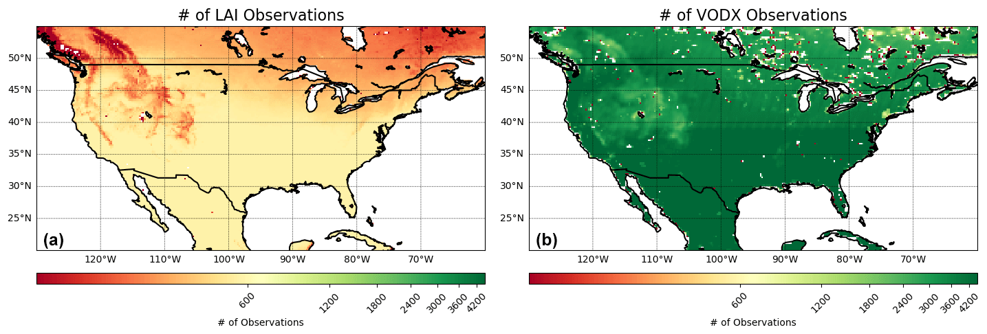
Figure 1Maps showing the cumulative number of observations provided for (a) CGLS LAI and (b) VODCA VODX over CONUS between 2003 and 2018. The color bar is on a log scale in order to show the vast differences between the two datasets.
VOD is comprised of attenuation from several components, primarily standing vegetation (which itself is composed of green leaf biomass, green structural biomass such as stems, and woody biomass such as trunks and branches), necromass (primarily litter), and water interception from rain or dew. VOD is separated into wavelength bands based on the radiation wavelengths from which it is derived. This study examines C-band (3.75 to 7.50 cm) and X-band (2.50 to 3.75 cm) VOD while also discussing L-band (15 to 30 cm) VOD. Recently, VOD has been more closely examined in regard to interacting effects of vegetation dynamics. A deeper look into L-band VOD by Konings et al. (2016) revealed that it is proportional to total vegetation water content, and the authors tweak their retrieval algorithm to more accurately account for vegetation effects on soil moisture observations.
This study uses the X-band of the newly created Vegetation Optical Depth Climate Archive (VODCA) (Moesinger et al., 2020). VODCA is a synthesis of various satellite sensors from 1987 and uses the Land Parameter Retrieval Model (LPRM) V6, which simultaneously retrieves and calculates soil moisture and VOD from horizontally and vertically polarized microwave observations (Mo et al., 1982; Meesters et al., 2005; Owe et al., 2008; van der Schalie et al., 2017). The dataset is compiled from the AMSR-E, AMSR2, SSM/I, TMI, and WindSat sensors and separates the syntheses into C-, X-, and Ku-band VOD retrievals. Ku-band VOD from VODCA did not encompass the entire period of interest in this study, stopping in 2017. While both the C- and X-band VOD may suitably represent vegetation over a wider array of land cover, X-band VOD was ultimately chosen to be assimilated in this study as Kumar et al. (2020) found large improvements in ET estimations from X-band VOD assimilation relative to C-band VOD. Because the TMI sensor aboard the Tropical Rainfall Measuring Mission (TRMM) satellite is in a 35∘ inclination orbit and thus does not encompass the entirety of the CONUS domain and because, in the X-band of VODCA, TMI is the only sensor between 1998 and late 2002, the year 2003 was chosen as a starting point in order to have full-domain observations.
Each sensor source in VODCA is first processed by removing locations known to be influenced by radio frequency interference (RFI); removing observations where land surface temperature (LST) is below freezing (as due to the changing dielectric permittivity of water and ice, the VOD cannot be accurately retrieved in frozen conditions); and removing negative values of VOD, which are data artifacts and not physically possible. Daytime retrievals were found to have higher errors than their nighttime counterparts, and thus only nighttime retrievals are used in VODCA. The sensor datasets are then individually matched based on the VOD band by using an improved cumulative distribution function matching scheme to correct for systematic differences between the sensors (details of the processing can be found in Moesinger et al., 2020). Finally, where multiple sensor observations are available, the bands are then merged via the arithmetic mean. This VODCA dataset is available globally at a spatial resolution. Due to the different number of sensors depending on each VOD band (and geographic location) and the timing of the satellite overpasses, the merged product provides observations for at least 40 % of all days with at least one sensor and upwards of 70 % with two or more.
Figure 2 shows the time series response of CGLS LAI (solid green line), VODCA X-band VOD (VODX) (dashed red line), and VODCA C-band VOD (VODC) (dotted blue line) near Lincoln, Nebraska, from 2003 to 2018. This pixel is composed primarily of C3 and C4 crops. LAI observations have a far more predictable and seasonal pattern. X-band VOD is also a stronger signal compared to C-band VOD. The peaks are relatively close in timing in this case but can also be offset due to the difference in peak vegetation water content. While this figure demonstrates that there is a correlation between LAI and VOD, it also shows that one cannot be substituted for the other.
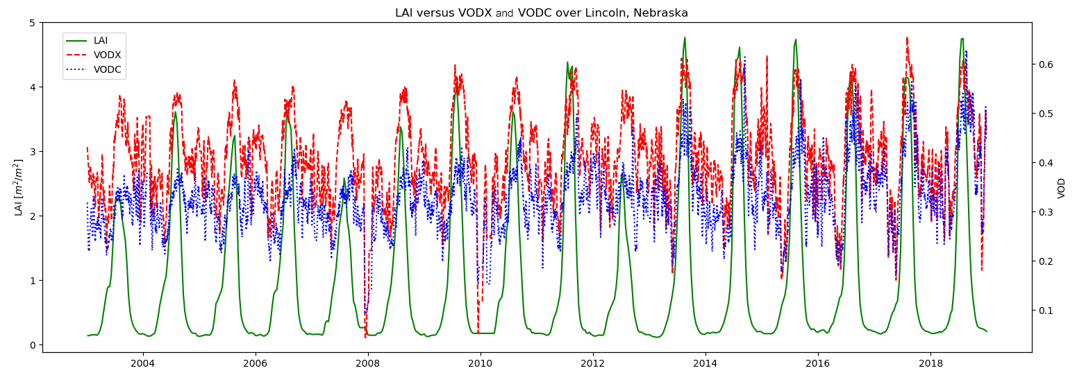
Figure 2A time series showing the response of CGLS LAI (solid green line), VODCA VODX (dashed red line), and VODCA VODC (blue, dotted) over Lincoln, Nebraska, from 2003–2018.
As was done in Kumar et al. (2020), VOD observations are seasonally linearly re-scaled to match observed LAI over the same period, in this case from the CGLS LAI dataset. Before linear re-scaling, the LAI and VOD observations are first scaled and matched to the same grid. A linear monthly re-scaling was then performed using a 3-month moving-window period to best match the two datasets over seasonal timescales. Over an entire year, this re-scaling is represented by 12 monthly equations, each taking into account the climatologies of the months preceding and succeeding it, and it is applied on a per-pixel basis. Each monthly equation is the same from one year to another. Each equation results from a first-order linear regression. In addition to this cumulative distribution function matching, a 30 d rolling average is applied after the re-scaling to smooth the resulting LAI proxy and allow for better performance of the assimilated data. VOD is sensitive to short-term changes in vegetation water content such as rainwater interception (Saleh et al., 2006). This day-to-day variability does not reflect changes in LAI.
For the sake of clarity regarding the re-scaling methodology, the Python code segment responsible for re-scaling of VOD values is given in the Supplement to this article.
Re-scaling is required because the ISBA LSM cannot simulate VOD directly, and thus we cannot assimilate VOD data directly into the model. As shown in the Fig. 2 time series, as well as what was demonstrated in Albergel et al. (2018a), LAI and VOD observations are correlated, and this relationship enables us to match the VOD to LAI observations and use the resulting product to assimilate in place of LAI in the model.
2.4 Independent evaluation observations
In addition to comparing the results to the assimilated data themselves, this study uses independent satellite-derived sources of evapotranspiration (ET), gross primary production (GPP), and in situ observations of SSM.
2.4.1 ALEXI evapotranspiration
Evapotranspiration (ET) is a broad term including many individual components and sources of evaporation and transpiration. These components include leaf transpiration, bare-soil evaporation, interception loss, surface water evaporation, and sublimation. ET is also strongly coupled with ecosystem production (Law et al., 2002), which in turn is driven by water availability (Noy-Meir, 1973). Therefore, measuring and predicting ET can be a valuable asset in terms of monitoring and predicting agricultural droughts.
The Atmosphere-Land Exchange Inverse (ALEXI) model is a surface energy balance model, which calculates evapotranspiration (ET) from a two-source land surface representation of the energy budget (Anderson et al., 1997, 2007a, b, 2011). The land surface is treated as a combination of soil and vegetation in the model, with each having unique temperatures, fluxes, and coupling with the atmosphere. Thermal infrared bands from the Geostationary Operational Environmental Satellite (GOES) sensors estimate land surface temperature (LST) and provide the driving force for ALEXI over the United States, with Meteosat Second Generation (MSG) providing data over Europe and Africa. Global products use the Geoland2 land cover database (Lacaze et al., 2010) to estimate LST. Regional vegetation cover is estimated from MODIS-derived LAI products. Aerodynamic and atmospheric boundary layer conditions are derived from North American Regional Reanalysis (NARR) (Mesinger et al., 2006), the Weather Research and Forecasting (WRF) model (Skamarock et al., 2005), and the Modern-Era Retrospective Analysis for Research and Applications (MERRA) (Gelaro et al., 2017) for the US, European–African, and global domains respectively. Finally, the University of Maryland's global land cover classification (Hansen et al., 2000) is used to define surface characteristics over all domains. The ALEXI ET product is available at a spatial resolution of globally and at over CONUS.
2.4.2 FLUXCOM gross primary production
Gross primary production (GPP) is a measure of CO2 assimilated into vegetation by photosynthesis. This sequestration of carbon plays an important role in the global carbon budget. GPP is indicative of vegetation conditions and photosynthetic activity and is highly coupled to water, light, and soil nutrient availability. However, direct, global measures of GPP are not currently possible (Anav et al., 2015) and instead must be estimated by measurements of carbon exchange between the land surface and the atmosphere.
The global FLUXNET network is a vast organization of eddy covariance towers used to measure trace gas fluxes between the biosphere and atmosphere (Jung et al., 2009; Pastorello et al., 2020). Machine learning algorithms are then applied to the energy and gas fluxes, as well as meteorological variables, to estimate fluxes in GPP and terrestrial ecosystem respiration (TER) (Reichstein et al., 2005; Baldocchi, 2008; Lasslop et al., 2010). This network of in situ measurements is then taken and combined with MODIS imagery for quality control and feature selection, put through several machine learning approaches, and finally combined with seasonal gridded satellite and meteorological observations to generate global carbon and energy flux products, FLUXCOM (Tramontana et al., 2016; Jung et al., 2018). This study uses the global GPP product from FLUXCOM to evaluate the performance of vegetation parameters independent from the LAI assimilated by LDAS-Monde. When this study was performed, the global FLUXCOM GPP data at a resolution were available from 1980 to 2013. It must be noted that there has been a word of caution that interannual variability patterns of FLUXCOM data may not be completely realistic (Jung et al., 2020).
2.4.3 United States Climate Reference Network
The United States Climate Reference Network (USCRN) is a sustained network of climate monitoring stations maintained by the National Oceanic and Atmospheric Administration (NOAA) National Centers for Environmental Information (NCEI) (Diamond et al., 2013; Bell et al., 2013). The network contains 114 stations in the contiguous USA and provides high-quality, long-term temperature, precipitation, solar radiation, wind speed, humidity, soil moisture, and soil temperature observations. This study uses the soil temperature and soil moisture observations, which are provided sub-hourly.
At each site, USCRN places three plots of probe units at five different depths: 5, 10, 20, 50, and 100 cm. The soil moisture probe measures the dielectric permittivity of the soil by observing reflected electromagnetic waves at 50 MHz, which is then converted to volumetric soil moisture (m3 m−3) via a calibration equation. Sensor calibration is also performed annually. A thermistor is also placed alongside the soil moisture sensor at all plots and depths. An average at each depth is calculated from the three plots every 5 min, and output data are typically publicly available within an hour of the reading. Figure 3 shows the locations of the USCRN in situ observations.

Figure 3Map illustrating the CONUS domain. Red dots represent the locations of the USCRN soil moisture stations.
Four sensor depths are selected and are matched to ISBA soil layers, 5 cm (WG3), 20 cm (WG_20), 50 cm (WG6), and 100 cm (WG8). This comparison uses the ISBA soil layers to directly compare against the point measurements of USCRN, but it is important to keep in mind that WG3, WG_20, WG6, and WG8 are layers of soil. WG3 is from 5 to 10 cm; WG_20 is a weighted average of WG4 and WG5 (as performed in Mucia et al., 2020) representing 10 to 40 cm; WG6 is a layer from 40 to 60 cm; and WG8 is the 80 to 100 cm layer.
This study compares USCRN data to LDAS-Monde soil moisture between the years of 2011 and 2018. While the network was operational as early as 2005, 2011 was selected as the start of the comparison in order to maximize the number of stations and homogenize the results of comparisons between stations.
2.5 Experimental setup and assessment
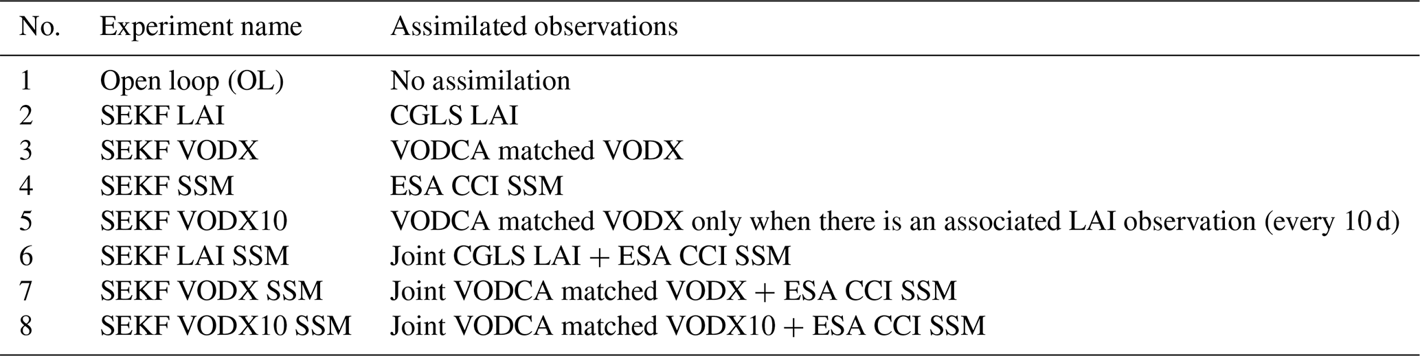
The experiments performed and reported in this study occur over the contiguous United States (CONUS) from 2003 to 2018 at a spatial resolution. This domain, as shown in Fig. 3, is defined by 20 to 55∘ N and 130 to 60∘ W. The year 2003 was chosen as the start date as this is approximately when the TRMM mission (containing the TMI sensor used in VODCA) ceases to be the only functioning VOD dataset included in VODCA. Because of the limited geographic extent of this mission (only up to 35∘ N), the analysis would be skewed. Table 2 provides the experiment names used throughout to reference the assimilation setups, and briefly describes what data are assimilated for each one. Besides the open loop (OL), SEKF LAI, SEKF VODX, SEKF SSM, SEKF LAI SSM, and SEKF VODX SSM, the SEKF VODX10 experiment was run at the same time, and this experiment uses VODX observations from VODCA as before, but it has filtered those observations to coincide only with where and when LAI observations from CGLS exist. This is used to test whether the changes produced between SEKF LAI and SEKF VODX are truly from the more frequent assimilation or from the quantifiable differences between matched VODX and LAI. If the SEKF VODX10 results closely resemble SEKF LAI results but SEKF VODX results are very different, this indicates the frequency of assimilated observations is the primary cause of those differences.
Table 2List of experiment names and their assimilated observations analyzed.
The primary statistical score used in this study is Pearson's correlation coefficient (r). The correlation is chosen as it is a simple yet effective measure of proximity to reference datasets. The average correlation as well as distribution of correlations can allow the quick assessment of improvement or degradation and is consistent with previous studies of LSMs and LSVs. Root mean square deviation (RMSD) was also calculated for the comparisons to reference observations, which gave the same results as with correlation and is thus not shown. In addition to the correlation, a normalized information contribution (NIC) is calculated for r as shown in Eq. (1):
This NICr, following Kumar et al. (2009), is normalized and thus allows for inter-comparison while accounting for differences between variables and regions.
When calculating correlation to satellite-based observations of LAI, ET, GPP, and SSM, the correlations are produced by combining all points in the domain into a single long time series, where the correlation is then computed against the observations processed in an identical way. This provides only one correlation score over the domain for each period. However, the significance of the score is strengthened due to the far larger sample length (15 years is considered over a large domain containing more than 20 000 pixels).
When analyzing the statistical scores of USCRN, several conditions are applied. First, frozen soil conditions are avoided by only calculating scores based on observations when temperature measurements are above 4 ∘C. As ISBA separately calculates frozen and liquid soil moisture, when conditions are close to freezing, there can be significant errors. Second, only stations with more than 100 observations (at the respective depths) are calculated for a sufficient number of data points. Finally, p values are calculated alongside the correlations, and stations without p values of significance, as defined by p >0.05, are screened out.
Bootstrapping is also used to calculate confidence intervals and thus determine statistical significance between different experiments. Essentially, bootstrapping is the repeated removal of random points in the dataset and recalculation of the desired score or variable. This study uses a constant 10 000 repeats to calculate the confidence intervals in order to generate a sufficiently large number of samples. In this study, bootstrapping is applied to the statistics calculated from USCRN.
For several analyses, probability distribution functions (PDFs) are estimated from the distribution of correlation scores of individual grid cells. These PDFs are derived using a Gaussian kernel density estimation, with “Scott's rule” calculating the appropriate smoothing bandwidth. These PDFs give a far smoother and readable estimation of correlations when compared to simple histograms. These PDFs are used in order to better visualize and compare the distribution of scores from several experiments at once, specifically to highlight smaller differences between experiments, which may not be easily seen in histograms. Figure S2a provides an example of a typical histogram along with panel (b) of the same figure, the accompanying PDF for the distribution of LAI correlations for different experiments over CONUS, demonstrating that they are in fact representing the same distribution.
3.1 Relationship between VOD and LAI
Before assimilating VOD observations, the X-band VOD (referred to as VODX from now on) data were compared against LAI observations, as well as LAI from the ISBA OL to determine their respective relationships. Additionally, VODX and LAI observations were analyzed over individual patch types, where more than 50 % of the patch represents a single vegetation type. These analyses provide more information regarding the strength of the VODX–LAI relationship over different vegetation types.
Figure 4 presents density scatterplots, representing all times and points when there is both VODX and LAI data over the growing seasons (April–September) of the 2003–2018 period. Linear regression and correlation scores have been plotted over the data. Logarithmic transformations to the VODX data were also applied (not shown) but with no significant increase in regression correlation or regression shape.
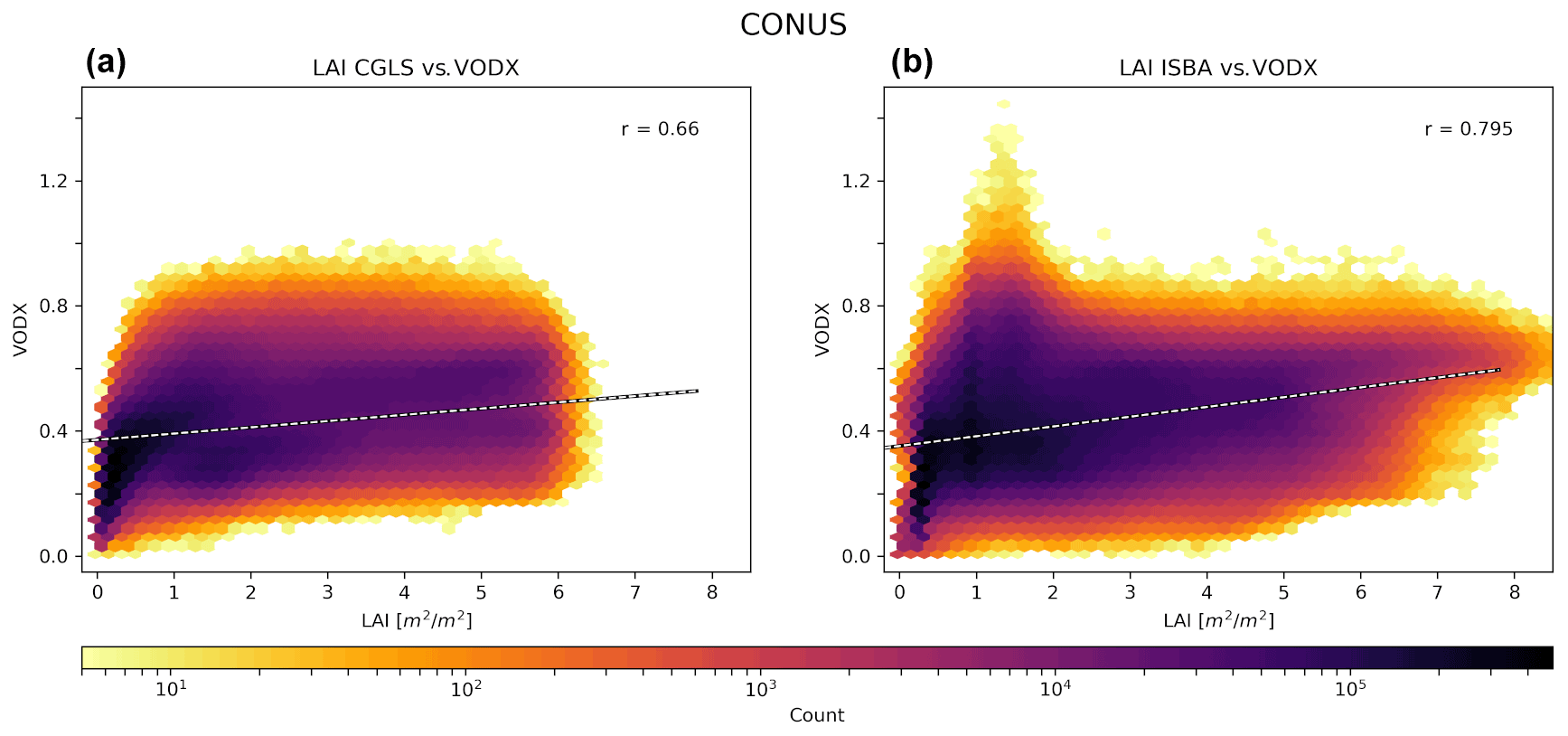
Figure 4Density scatterplots detailing the relationship between LAI and VODX from VODCA. This comparison only analyzes where and when there are both LAI and VOD observations. Warm colors represent more counts of points in the hexagonal bins. The color bar is logarithmically scaled in order to emphasize the distributions, and bins with under five counts are eliminated. A regression line and correlation score are added. This comparison only looks at points during the growing-season months (April–September) from 2003 to 2018. Panel (a) compares VODX to LAI from CGLS observations, while panel (b) compares VODX to LAI from the ISBA OL.
The LAI observations are moderately well correlated to VODX observations, as shown by the r value of 0.66. The relationship of VODX with LAI from ISBA (Fig. 4b) actually provides higher values, with an r of 0.80. Visually, we can see at higher LAI values that there is a more dramatic increase in VODX, whereas in Fig. 4a, the VOD values seem almost as if they flatten out above 1 m2 m−2 LAI. This is partly seen in Fig. 4b but is also slightly compensated for by progressively higher VOD, while eliminating low VOD values at high LAI. Additionally, Fig. 4b clearly shows certain artificial thresholds from ISBA, including the 0.3 m2 m−2 lower limit of LAI for most vegetation types and the 1 m2 m−2 lower limit for evergreen forests. These artifacts can be seen at a wide range of VOD values. These lower limits in ISBA are often reached in winter and spring months when vegetation activity and LAI are low, with the included spring months of April and May likely being the cause of this effect in Fig. 4. This figure reinforces the evidence that there is in fact a positive relationship between VOD and LAI observations.
When this same relationship of VODX observations versus LAI observations is performed over dominant patch types (according to ECOCLIMAP-SG), new insight is gained into vegetation types where the two variables are far more closely linked. Figure 5 displays density scatterplots of the observations of VODX compared to LAI observations over six ECOCLIMAP-SG patch types, namely (a) deciduous forests, (b) coniferous forests, (c) C3 crops, (d) C4 crops, (e) C3 grasslands, and (f) irrigated crops. Areas with higher density (i.e., higher concentrations of observations of LAI and VOD) are in darker colors. Spatial averages of when LAI and VOD observations are compared are also displayed with colored dots (approximately 1 dot per LAI observation) representing the season in which they were observed, with winter (cyan), spring (green), summer (red), and autumn (yellow).

Figure 5Density scatterplots detailing the relationship between LAI and VODX from VODCA over six dominant vegetation types: (a) deciduous forests, (b) coniferous forests, (c) C3 crops, (d) C4 crops, (e) C3 grasslands, and (f) irrigated crops for the years 2003 to 2018. Dominant vegetation is defined as where 50 % or more of a patch contains a single vegetation type. Higher concentrations of points trend towards black. Colored dots represent the spatial average over the four seasons, where cyan is winter, green is spring, red is summer, and yellow is autumn. Dashed black-and-white lines represent the linear regression of the seasonal scores.
Overall, for most vegetation types, there is a moderate positive correlation between the two observations. The notable exceptions are coniferous forests and irrigated crops, which produce negative or near-zero correlations. The seasonality does play a strong part as well, and the figure panels show a clear separation of values according to seasons over the patches. Winter correlations are typically low for all vegetation types, and the cyan seen in the graphs is often clumped at low LAI values. Spring scores are on average increased and contain a far wider range of LAI values but similar range of VOD values. Summer and autumn see the highest correlation scores and are characterized by a wider range of LAI and VOD values. Notably, deciduous forests have a negative correlation during summer months, but the autumn correlation is strongly positive.
The same analysis by patch is also performed using matched VODX in place of VODX observations. This matched VODX is the product of the seasonal linear re-scaling transformation of the observations into an LAI proxy. As is demonstrated in Fig. 6, the correlations are very strongly improved over the non-matched observations. Even so, a seasonal hysteresis pattern emerges over C3 and C4 crop patches, where autumn (yellow) matched VODX is visibly higher than at the same LAI values compared to other seasons. This transition from VODX to matched VODX shows that the transformation is viable and strongly improves the correlation. This matched VODX product is able to be assimilated as an LAI proxy into LDAS-Monde.
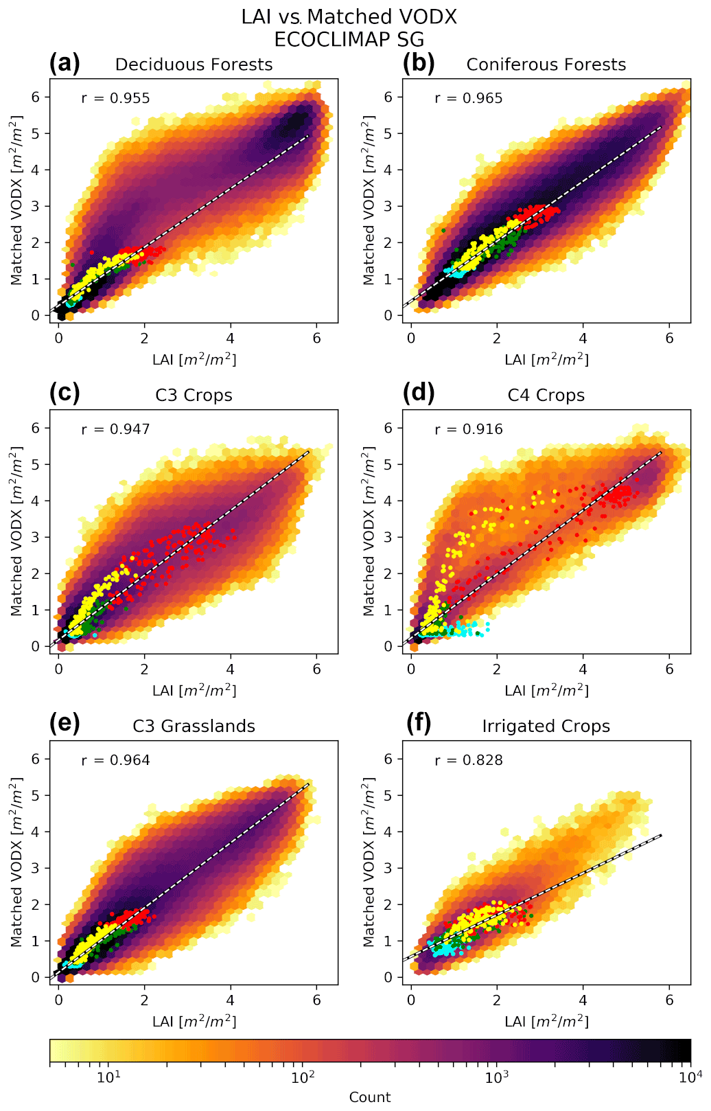
Figure 6Density scatterplots detailing the relationship between LAI and matched VODX from VODCA over six dominant vegetation types: (a) deciduous forests, (b) coniferous forests, (c) C3 crops, (d) C4 crops, (e) C3 grasslands, and (f) irrigated crops for the years 2003 to 2018. Dominant vegetation is defined as where 50 % or more of a patch contains a single vegetation type. Higher concentrations of points trend towards black. Colored dots represent the spatial average each time an LAI–VOD comparison is made over the four seasons, where cyan is winter, green is spring, red is summer, and yellow is autumn. Dashed black-and-white dashed lines represent the linear regression of the seasonal scores.
This seasonal linear re-scaling does come with some drawbacks however, including the merging of observed errors from the LAI and VOD as well as errors produced by the re-scaling, but this simple transformation does provide the opportunity to study more frequent assimilation of observations in place of LAI using a readily available dataset.
3.2 Impact of assimilating matched VOD
3.2.1 Assessment with satellite-derived observations
This section analyzes the impact of using and assimilating matched VODX as an LAI proxy in the LDAS-Monde system. For this analysis, the primary variables of interest are LAI, GPP, ET, and SSM. Out of the four, GPP, ET, and SSM are the truly independent datasets to compare to when investigating the assimilation of LAI or VODX. Most of the main conclusions are then drawn from the analysis of these variables. Comparisons to LAI observations are still presented, but as the LAI was used in the assimilation itself or to re-scale the VOD, it acts more as a benchmark for the assimilation.
The average monthly correlations are presented in Fig. 7 for the OL, SEKF LAI, SEKF VODX, and SEKF VODX10. First looking at LAI, Fig. 7a, the whole CONUS domain sees added value during the months of May through September when assimilating matched VODX in place of LAI. For the rest of the year, the scores for SEKF VODX are slightly below those of SEKF LAI. The improvement in LAI correlation from assimilating VODX comes as a slight surprise as this is in comparison to the CGLS LAI observations that themselves were assimilated in SEKF LAI. Some potential explanations include the far more frequent assimilation of VOD during the summer months when LAI is most rapidly changing. The results of SEKF VODX10 also show definitively that it is the more frequent observations and not the differences between LAI and matched VOD that are causing some improvement as SEKF VODX10 is consistently lower than both SEKF LAI and SEKF VODX throughout the year. Additionally, this panel shows that any assimilation of VODX or LAI significantly improves correlations compared to the model by itself (OL).

Figure 7Graphs of monthly correlations over CONUS between the LDAS-Monde OL (solid blue line), SEKF LAI (solid green line with star markers), SEKF VODX (solid red line with cross markers), and SEKF VODX10 (dash-dotted maroon line) and satellite-derived observations of (a) LAI (2003 to 2018), (b) GPP (2003 to 2013), (c) ET (2003 to 2018), and (d) SSM (2003 to 2018).
For the variable of GPP, Fig. 7b, some similar trends are seen. During the months of March through July, the assimilation of VODX performs far better than SEKF LAI or SEKF VODX10. From July to October, there is also some improvement but not as strongly as in the spring and early summer. Interestingly, for the OL, SEKF LAI, and SEKF VODX10, there is a visible dip in correlation scores during the month of May, while SEKF VODX sees near-constant or even slightly higher correlations compared to previous and future months. On average, the month of May sees some of the fastest vegetation change of the year for CONUS. The assimilation of observations at best every 10 d may not provide sufficient constraint to the vegetation during this period of rapid change. The near-daily VODX products provide more constraint and thus seem to immediately prove their utility in their use as LAI proxies for data assimilation. The changes in correlations between experiments and GPP observations are not as drastic as seen in LAI, but they do show the same overall trends. And importantly, this GPP observation is an independent evaluation of vegetation conditions, where the largest improvements from VOD assimilation are observed in the spring and summer months when droughts and heat waves are most likely to damage agricultural production.
With the ET variable, Fig. 7c, it is harder to view differences as the correlation scores for all the experiments seen here are relatively close. The only easily distinguishable differences arise in the months of May to August. During these months, like with LAI and GPP, SEKF VODX has the highest correlations. It is followed by SEKF LAI and SEKF VODX10, which are close to one another, then finally by the OL. In general, these correlation scores are lower than for LAI or GPP but are at their peak during much of the summer, when evaporative demand is highest and when it is critical for agricultural production to account for hot and dry conditions.
With SSM, Fig. 7d, correlations between the experiments are nearly indistinguishable except for some summer months, namely June through August. Overall correlations are very high, consistently higher than 0.80, and, contrary to all the other variables, provide the best correlations in winter months. Where we do see differences between the experiments between June and August, it can be noted that the OL actually performs the best, followed by SEKF LAI and SEKF VODX10, and finally the lowest scores are given to SEKF VODX. While in absolute terms these differences are small, a logical explanation can support these rankings: any data assimilation in LDAS-Monde, whether it is of vegetation such as LAI or VOD or of SSM, directly changes the eight control variables. Seven of these variables are soil moisture, with six of them deeper than the 5 cm WG3 layer used to compare against these ESA SSM observations. The assimilation, of LAI or VODX in this case, impacts all these layers and can adjust the uppermost layer used here to coincide with higher LAI values. In these experiments, only the vegetation variable is assimilated, and thus there is no secondary compensation at the upper soil levels done by assimilating SSM observations.
The PDFs (derived from the histogram of correlation scores) are given in Fig. 8 over CONUS. LAI, Fig. 8a, provides a very clear indication that the assimilation of vegetation variables, whether LAI or VODX, heavily shifts the distribution of correlations higher. From correlations of 0.10 to 0.45, SEKF VODX has slightly more points than SEKF LAI, and this is reversed from 0.45 to 0.75. SEKF VODX then quickly spikes at a correlation value of 0.88, with SEKF LAI shifted higher, and a peak closer to 0.90. These strongly changed values from the OL and similarities between SEKF LAI and SEKF VODX demonstrate even more that VODX can properly act as an LAI proxy.
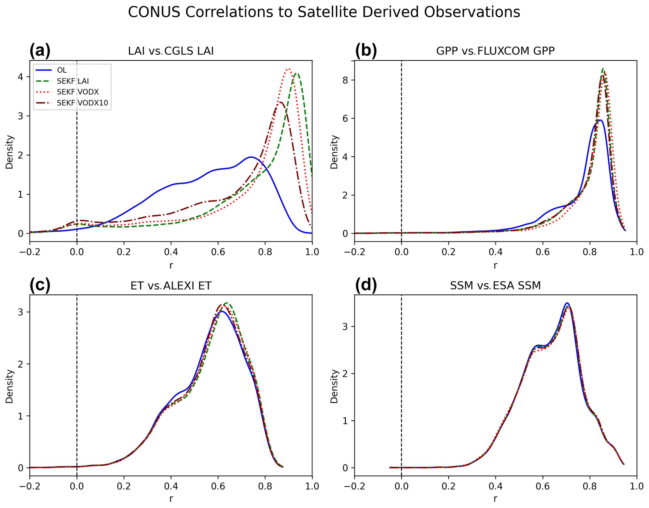
Figure 8Graphs of probability distribution function (PDF) correlation distributions over CONUS between the LDAS-Monde OL (solid blue line), SEKF LAI (dashed green line), SEKF VODX (dotted red line), and SEKF VODX10 (dash-dotted maroon line) and satellite-derived observations of (a) LAI (2003 to 2018), (b) GPP (2003 to 2013), (c) ET (2003 to 2018), and (d) SSM (2003 to 2018). The PDFs were calculated using a Gaussian kernel density estimation of the scores. The kernel density estimation smoothing bandwidth is calculated using the default Scott's rule.
The distributions of GPP correlations, Fig. 8b, are not as widespread as LAI; however, a clear pattern still emerges. Starting at 0.40, SEKF LAI and SEKF VODX have fewer grid cells than the OL, which lasts until around 0.80. It is around this point that the shift towards greater number of higher correlation points with SEKF LAI and SEKF VODX is strongly apparent. While very similar, SEKF VODX does slightly outperform SEKF LAI in this case as well, having a greater number of higher correlation values.
Like with the monthly correlations presented before, the distribution of ET scores, Fig. 8c, is very similar between all the experiments. At around 0.40, there is a noticeable difference where SEKF VODX and SEKF LAI begin to contain fewer points, which is then made up by those experiments having a greater number of higher values consistently between 0.55 and 0.70. At their peak densities, SEKF LAI slightly outperforms SEKF VODX, but SEKF VODX still improves on the OL.
For all displayed experiments, the distribution of SSM correlation scores in Fig. 8d is almost bimodal. There is one peak at 0.55 and another between 0.70 and 0.80. The experiments of SEKF LAI and SEKF VODX are only slightly different, with both edging out the OL in terms of performance. SEKF VODX also edges out SEKF LAI, again with a slightly larger number of high correlations.
3.2.2 Assessment with in situ observations
The comparison of LAI, GPP, ET, and even SSM against satellite-derived observations serves an important purpose, as those observations are spatially continuous. However, errors in the sensors or processing of the data still exist, and relatively large spatial resolutions mean losses of more localized information. With this in mind, all of the experiments listed in Table 2 are also compared to soil moisture observations from the United States Climate Reference Network (USCRN) in situ soil moisture monitoring stations.
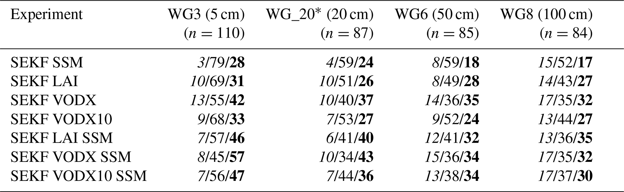
Table 3 provides the average correlations to the in situ stations for each of the experiments and at each of the depths. As previously seen in Mucia et al. (2020), correlations strongly drop as the depths become lower. To two significant figures, the correlations at 5 cm are all identical at 0.75. There is very slightly more variability at lower depths with 20 cm scores ranging from 0.68 for the OL to 0.70 for all the experiments jointly assimilating vegetation and soil moisture observations. Similar variations are present for the 50 and 100 cm depths. Notably, the 100 cm scores are all the same at 0.48 except for the OL and SEKF SSM experiments with 0.46.
Table 3Average correlations scores between USCRN in situ soil moisture observations and LDAS-Monde soil moisture at 5, 20, 50, and 100 cm depths. Bold values indicate the highest score at each depth.

*WG_20 is a weighted average of WG4 and WG5 in order to directly compare to 20 cm observations from USCRN.
Statistical bootstrapping was performed on all the calculated values, before rounding significant figures, to calculate the upper and lower bounds of the 95 % confidence intervals (CIs). The resulting CIs showed that at every depth, all the experiments' mean correlations were within every CI, meaning no experiment could be said to be statistically different from any other at the same depth.
Seen throughout these results is the changing number of stations (n) used in the analyses. The 5 cm comparisons have 110 stations, 20 cm uses 87 stations, 50 cm uses 85 stations, and 100 cm uses 84 stations. This is simply due to the fact that USCRN cannot install soil moisture or soil temperature probes in hard or rocky ground layers, as stated in the USCRN soil climate observations documentation (NCEI NOAA, 2022). In all cases, the 5 and 10 cm probes are installed, but deeper layers depend on the regolith type.
To better analyze differences on a more individual scale, the normalized information contribution of the correlations (NICr) were calculated for each experiment and each depth in comparison to the OL. These NICr values tell us by how much the assimilation experiments improved or degraded scores in respect to the OL. Table 4 displays each experiment and depth and the number of stations that were degraded (italics), neutral, and improved (bold). This approach avoids averaging scores (which can be strongly impacted by smaller numbers of extreme scores) while still providing a performance overview of the whole domain.
Table 4Number of degraded (italics)/neutral/improved (bold) USCRN stations after assimilation using NICr between the OL and various LDAS-Monde experiments at 5, 20, 50, and 100 cm depths. Stations are considered improved if the NICr is greater than 3, degraded if the score is less than 3, and neutral if it is between −3 and 3.
*WG_20 is a weighted average of WG4 and WG5 in order to directly compare to 20 cm observations from USCRN.
In a similar manner, Fig. 9 displays the PDF of the distribution of differences in correlation for each of the four depths compared to the OL and looks at the responses of the SEKF SSM, SEKF LAI, SEKF VODX, SEKF LAI SSM, and SEKF VODX SSM experiments.
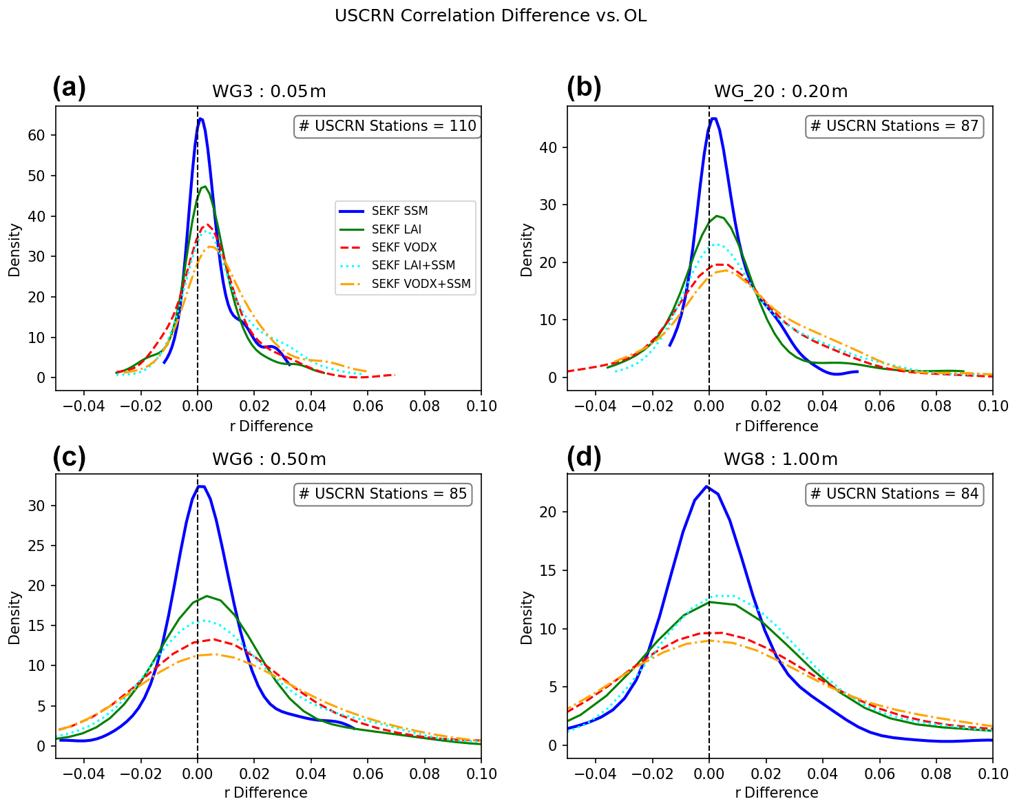
Figure 9Probability distribution functions of the distribution of correlation differences between the OL and SEKF SSM (solid bold blue line), SEKF LAI (solid green line), SEKF VODX (dashed red line), SEKF LAI SSM (dotted cyan line), and SEKF VODX SSM (dash-dotted orange line) for USCRN at (a) WG3 (5 cm), (b) WG_20 (20 cm), (c) WG6 (50 cm), and (d) WG8 (100 cm) between 2011 and 2018.
In regard to the impact of assimilating re-scaled VOD in lieu of LAI, the NICr scores, based on the in situ observations, provide evidence that SEKF VODX and SEKF LAI are similar and comparable. SEKF VODX increases the number of improved stations compared to SEKF LAI at all depths while also keeping constant or slightly increasing the number of degraded stations. The improved stations outnumber the degraded ones at all depths. Additionally, the SEKF VODX10 experiment shows stronger similarities to SEKF LAI than to SEKF VODX, indicating that the differences are due to the more frequent assimilation of VODX. These results demonstrate that re-scaled VODX can indeed be a suitable substitute for LAI in LDAS-Monde.
3.3 Impact of individual and joint assimilation of vegetation variables and SSM
While previously discussed above when assessing correlations and NICr for USCRN, this section will go into more detail regarding the effects of jointly assimilating variables of vegetation (LAI or matched VODX) and SSM in LDAS-Monde. We have already seen that the joint assimilation provides a noticeable increase in improved USCRN stations relative to the OL, over the single assimilation of vegetation variables or SSM.
Figure 10 presents the same type of figure as previously, looking at the monthly scores of four LSVs of interest over CONUS but including the joint assimilation experiments of SEKF LAI SSM and SEKF VODX SSM. The main concern in this figure and the following text is determining the improvement, if any, between the solid (single assimilation) and segmented (joint assimilation) red and green lines. As seen in panel (a), there is no discernible difference between the single and joint assimilation for LAI. But as panels (b) and (c) show, jointly assimilating vegetation and SSM produces slightly improved monthly correlations over the whole CONUS domain for GPP and ET respectively. These improvements are primarily seen in the months of June through August, and while the changes are small, they indicate consistent improvements over the single assimilation of LAI or matched VODX. Regarding the variable of SSM, the joint assimilation strongly improves the monthly correlations from LAI to LAI SSM and from VODX to VODX SSM. To reiterate, because the SSM observations assimilated are the same used for comparison in panel (d), it is merely an indication that the data assimilation is truly shifting model soil moisture values closer to those of observations.

Figure 10Graphs of monthly correlations over CONUS between the LDAS-Monde OL (solid blue line), SEKF SSM (dash-dotted cyan line), SEKF LAI (solid green line with star markers), SEKF VODX (solid red line with cross markers), SEKF LAI SSM (dashed green line), and SEKF VODX SSM (dotted red line) and satellite-derived observations of (a) LAI (2003 to 2018), (b) GPP (2003 to 2013), (c) ET (2003 to 2018), and (d) SSM (2003 to 2018).
When assessing with in situ observations, both the NICr table and PDFs, the 5 cm changes are the strongest, with SEKF VODX SSM providing the highest number of improved stations while having some of the lowest number of degraded stations. SEKF LAI SSM and SEKF VODX10 SSM perform similarly but with a reduction in improved stations. Assimilating just LAI, VODX, or VODX10 consistently under-performs in terms of their matching joint assimilation experiments by increasing the number of degraded stations while having fewer improved stations. And finally, SEKF SSM, while showing the fewest degraded stations, also has the fewest improved. As depths get lower, the numbers become closer. It is generally still seen that the joint assimilation of vegetation and soil moisture improves more stations than the individual assimilation, and the number of stations degraded stays similar. These trends go to show that the joint assimilation has distinct added value in soil moisture monitoring and will be discussed in more detail in the following sections.
Overall, the use of the USCRN in situ observations agrees with the hypothesis that the assimilation of vegetation has stronger effects on soil moisture in the root zone than the assimilation of SSM. It also goes to show that the assimilation of VODX is on a par with or even an improvement on the assimilation of LAI.
4.1 Analysis of re-scaled X-band VOD as an LAI proxy
In the comparison of VOD and LAI before seasonal linear re-scaling, it is immediately apparent that vegetation type plays a large role in their relationship. These values seen and described in the results seem to indicate that heavily forested regions have only weak correlations between VOD and LAI observations. In this research, the improvements to GPP from the assimilation of X-band VOD can be explained by a better sensitivity of X-band VOD to the leaf biomass.
While direct assimilation of VOD may be possible in some data assimilation systems (such as L-band VOD in CCDAS, as performed by Scholze et al., 2019), this is not possible in LDAS-Monde, as the NIT version of ISBA simulates neither wood biomass nor specific leaf area (SLA), both necessary for simulating VOD. Additionally, the objective of VOD data assimilation in CCDAS is to constrain certain model parameters, while the objective of assimilating re-scaled X-band VOD in LDAS-Monde is to sequentially assimilate observations in order to constrain the day-to-day trajectory of the ISBA state variables, without changing model parameter values. Although ISBA is an uncalibrated model, it performs as well as other state-of-the-art models in inter-comparison experiments (e.g., Fig. B2 in Friedlingstein et al., 2020), even without assimilation. Moreover, studies have shown that VOD may be sensitive to rainwater interception by leaves (e.g., Saleh et al., 2006). The ISBA model is able to simulate interception, but there is no simple way to simulate the physical interception effect on VOD. It is for this reason that a statistical re-scaling of VOD towards an LAI proxy was pursued.
After seasonal linear re-scaling the VOD to match the LAI observations, hysteresis patterns over C3 and C4 crops emerged. Due to these patches being dominated by cultivated vegetation, it is possible that heavier ground litter during and after harvesting produces a stronger VOD response while at lower LAI. This effect is more apparent in C4 crops potentially due to their overall higher LAI and VOD values. Leaf water interception, on both growing plants and ground litter, could also disproportionately increase the VOD observations, leading to an offset. Future studies could include filtering and analyzing this LAI–VOD relationship, accounting for leaf water interception. Additionally, VOD being more strongly related to leaf biomass than to LAI could lead to a non-constant LAI-to-VOD ratio. This ratio could be related to SLA, as pointed out by Shamambo et al. (2019). This effect would be most marked over near-uniform vegetation types, including some unmixed forests and many crops, and would emerge during the growing season. This matches the observed hysteresis most strongly seen in areas dominated by C3 and C4 crop types and in the growing seasons of spring and summer found in this study. Yet another explanation could be linked to the surface roughness. Fernandez-Moran et al. (2015) and Hornbuckle et al. (2016) found that satellite microwave retrievals are impacted by surface roughness as well as vegetation water content and soil moisture. As management decisions for agricultural producers can impact a field's roughness (i.e., by plowing or tilling), it is possible that higher values of microwave retrievals and ultimately VOD may be at least partially explained by a higher roughness. Further analysis of LAI and VOD over agricultural lands of varying roughness could be conducted to move towards better understanding this phenomenon.
4.2 Does the assimilation of matched VOD improve LDAS-Monde's ability to monitor drought?
After assimilation, the SEKF VODX experiment provided either comparable or improved seasonal representation of GPP and ET, two important LSVs with regard to agricultural droughts. The distribution of correlations for these LSVs also confirms that the assimilation of VODX provides approximately equal or improved correlations to GPP and ET over this domain. With the assessment with the in situ USCRN, this idea is strengthened as SEKF VODX provided more improved stations at all soil depths. And even though the average correlations were statistically indistinguishable, the trend still showed some improvement on SEKF VODX. Further studies comparing to in situ soil moisture with a stronger significance would be a suitable follow-up to solidify this trend.
4.3 Does the joint assimilation of vegetation variables and soil moisture provide better initial conditions?
Over the entire CONUS domain, there is evidence indicating added value for GPP and ET variables from joint vegetation and soil moisture assimilation. In conjunction with the results from the USCRN analysis, joint assimilation does, overall, show more potential value than assimilation of vegetation-related variables and few, if any, drawbacks. Additionally, it is shown that the assimilation of vegetation, be it LAI or matched VODX, has a far stronger impact on the LSVs of LAI, GPP, and ET compared to the assimilation of SSM.
The small impact of assimilating SSM can be explained by the fact that we use a state-of-the art land surface model able to represent diffusion processes into the soil with many layers. In dry conditions, the simulated SSM is decoupled from soil moisture of deeper soil layers. As a result, assimilating SSM has a limited impact on the model state variables (Parrens et al., 2014). On the other hand, directly assimilating LAI impacts deep soil layers, and a more efficient analysis of root zone soil moisture can be performed than by assimilating SSM alone (see also Fig. 4 in Albergel et al., 2017). The detrimental effect on the assimilation of decoupling of surface soil moisture was described in past studies and is not specific to the ISBA LSM. For example, Capehart and Carlson (1997) showed that decoupling is caused by strong evaporation rates, with or without vegetation cover. However, a limitation of the standard version of ISBA used in this study is that a single composite soil–vegetation energy budget is used and the effect of plant residues on evaporation and on surface temperature is not represented. A new version of the ISBA model includes a multiple energy budget together with a representation of litter in forests (Napoly et al., 2017) that will be generalized to low vegetation in the next version of SURFEX. Using this new capability could improve the benefit of assimilating SMOS (Soil Moisture And Ocean Salinity), SMAP (Soil Moisture Active Passive) or ASCAT (Advanced Scatterometer) SSM retrievals or level-1 observations.
Another step in the direction of improving initial conditions consists of directly assimilating level-1 data, such as ASCAT radar backscatter or microwave brightness temperature from passive instruments into LDAS-Monde. This would allow the use of all the information contained in the signal, including soil moisture and vegetation, and at the same time reduce observations errors in the data assimilation (Shamambo et al., 2019; Shamambo, 2020). A major step in this development is the solution of the observation operator, and current steps towards developing this operator are focused on using machine learning approaches to find the optimal term.
By improving initial conditions of the LDAS, next steps also include testing drought forecasting by combining these known improvements through more frequent and joint assimilation of observations with LDAS-Monde's forecast capacity. The analysis of drought forecast accuracy and potential warning time could prove useful for agricultural managers and stakeholders.
This study finds a generally positive relationship between observations of LAI and VODX. This relationship still contains variability, strongly linked to dominant vegetation. These results agrees with previous work comparing vegetation cover and conditions to VOD. Coniferous forests consistently had the weakest correlation, while C3 and C4 crops typically had the best. Seasonality also dramatically changed the LAI–VODX relationship, with winter scores typically the lowest and summer and autumn correlations typically the strongest. Matched VODX was far more strongly correlated to LAI observations than non-matched VODX, as expected, but still exhibited significant variation.
This study then demonstrated the utility of the assimilation of microwave X-band VOD into LDAS-Monde, as well as showing a slight advantage by using a joint assimilation of vegetation-related observations (VOD or LAI) in combination with SSM. This assessment over the United States showed improved representation of ET and GPP, compared to independent observations, over some months' assimilation of VOD. The improvements seen in GPP and ET correlations by assimilating matched VODX in place of LAI are almost entirely due to the more frequent observations of VOD. This is shown because the experiment SEKF VODX10, which assimilated matched VODX at the same frequency as LAI observations, performs considerably worse than the natural VODX observation frequency.
Using in situ observations of soil moisture, the joint assimilation of vegetation-related observations and SSM reduced the number of degraded correlations while increasing the number of improved stations for the top 20 cm of soil. Additionally, when assessing the RZSM, the assimilation of SSM by itself proved to be weaker than that of vegetation (LAI or VOD) alone, even at the uppermost layers of soil.
Follow-up studies will bring these improvements into the LDAS-Monde forecast configuration and will investigate the capability of early detection and warning of drought events.
LDAS-Monde is a part of the ISBA land surface model and is available open source via the surface modeling platform called SURFEX. SURFEX can be downloaded freely at http://www.umr-cnrm.fr/surfex/data/OPEN-SURFEX/open_surfex_v8_1_20210914.tar.gz (last access: 5 May 2022; CNRM, 2016) using a CeCILL-C license (a French equivalent to the LGPL; http://cecill.info/licences/Licence_CeCILL_V1.1-US.html, last access: 5 May 2022; CEA et al., 2013). It is updated at a relatively low frequency (every 3 to 6 months). If more frequent updates are needed or if what is required is not in Open-SURFEX (Dr Hook, FA/LFI formats, Gaussian grid), you are invited to follow the procedure to obtain an SVN account and to access real-time modifications of the code (see the instructions via the first link). The developments presented in this study stemmed from SURFEX version 8.1. LDAS-Monde technical documentation and contact points are freely available at https://opensource.umr-cnrm.fr/attachments/2961/OpenLdasMonde_V2.0.tar.gz (last access: 5 May 2022; CNRM, 2019).
ERA5 data are available from Hersbach et al. (2018) (https://doi.org/10.24381/cds.adbb2d47), CCI SSM from the ESA Climate Office (https://doi.org/10.5285/0683e320d8634a37aa1d9ef62dd41a0d, Dorigo et al., 2020; https://data.ceda.ac.uk/neodc/esacci/soil_moisture/data/daily_files/COMBINED/v04.7, last access: 5 May 2022), CGLS LAI from Copernicus (https://land.copernicus.vgt.vito.be/PDF/portal/Application.html#Browse;Root=512260;Collection=1000083;Time=NORMAL,NORMAL,-1,,,-1,,, last access: 5 May 2022; Copernicus, 2020), VODCA from Zenodo (https://doi.org/10.5281/zenodo.2575599, Moesinger et al., 2019), USCRN soil moisture observations from NOAA (https://www.ncei.noaa.gov/access/crn/qcdatasets.html, last access: 5 May 2022; NCEI NOAA, 2022), and FLUXCOM GPP from https://www.fluxcom.org/ (last access: 5 May 2022; FluxCom, 2022).
The supplement related to this article is available online at: https://doi.org/10.5194/bg-19-2557-2022-supplement.
AM, CA, and JCC conceptualized the project. AM led the investigation, determined the methodology, and wrote the original draft of the paper. All co-authors contributed to the review and editing of the paper.
The contact author has declared that neither they nor their co-authors have any competing interests.
Publisher’s note: Copernicus Publications remains neutral with regard to jurisdictional claims in published maps and institutional affiliations.
This article is part of the special issue “Microwave remote sensing for improved understanding of vegetation–water interactions (BG/HESS inter-journal SI)”. It is a result of the EGU General Assembly 2020, 3–8 May 2020.
The authors would like to thank Martha Anderson (USDA) and Christopher Hain (NASA) for kindly providing the ALEXI data.
This research has received funding from the French Make Our Planet Great Again PhD program of 2018 (grant no. 927908C) and from the European Union Horizon 2020 research and innovation program (grant agreement no. 958927 (CoCO2)).
This paper was edited by Matthias Forkel and reviewed by two anonymous referees.
Albergel, C., Calvet, J.-C., Mahfouf, J.-F., Rüdiger, C., Barbu, A. L., Lafont, S., Roujean, J.-L., Walker, J. P., Crapeau, M., and Wigneron, J.-P.: Monitoring of water and carbon fluxes using a land data assimilation system: a case study for southwestern France, Hydrol. Earth Syst. Sci., 14, 1109–1124, https://doi.org/10.5194/hess-14-1109-2010, 2010. a
Albergel, C., Munier, S., Leroux, D. J., Dewaele, H., Fairbairn, D., Barbu, A. L., Gelati, E., Dorigo, W., Faroux, S., Meurey, C., Le Moigne, P., Decharme, B., Mahfouf, J.-F., and Calvet, J.-C.: Sequential assimilation of satellite-derived vegetation and soil moisture products using SURFEX_v8.0: LDAS-Monde assessment over the Euro-Mediterranean area, Geosci. Model Dev., 10, 3889–3912, https://doi.org/10.5194/gmd-10-3889-2017, 2017. a, b, c, d, e, f
Albergel, C., Dutra, E., Munier, S., Calvet, J.-C., Munoz-Sabater, J., de Rosnay, P., and Balsamo, G.: ERA-5 and ERA-Interim driven ISBA land surface model simulations: which one performs better?, Hydrol. Earth Syst. Sci., 22, 3515–3532, https://doi.org/10.5194/hess-22-3515-2018, 2018a. a
Albergel, C., Munier, S., Bocher, A., Bonan, B., Zheng, Y., Draper, C., Leroux, D., and Calvet, J.-C.: LDAS-Monde Sequential Assimilation of Satellite Derived Observations Applied to the Contiguous US: An ERA-5 Driven Reanalysis of the Land Surface Variables, Remote Sens., 10, 1627, https://doi.org/10.3390/rs10101627, 2018b. a
Albergel, C., Dutra, E., Bonan, B., Zheng, Y., Munier, S., Balsamo, G., de Rosnay, P., Muñoz-Sabater, J., and Calvet, J.-C.: Monitoring and Forecasting the Impact of the 2018 Summer Heatwave on Vegetation, Remote Sens., 11, 520, https://doi.org/10.3390/rs11050520, 2019. a, b
Albergel, C., Zheng, Y., Bonan, B., Dutra, E., Rodríguez-Fernández, N., Munier, S., Draper, C., de Rosnay, P., Muñoz-Sabater, J., Balsamo, G., Fairbairn, D., Meurey, C., and Calvet, J.-C.: Data assimilation for continuous global assessment of severe conditions over terrestrial surfaces, Hydrol. Earth Syst. Sci., 24, 4291–4316, https://doi.org/10.5194/hess-24-4291-2020, 2020. a, b, c
Anav, A., Friedlingstein, P., Beer, C., Ciais, P., Harper, A., Jones, C., Murray-Tortarolo, G., Papale, D., Parazoo, N. C., Peylin, P., Piao, S., Sitch, S., Viovy, N., Wiltshire, A., and Zhao, M.: Spatiotemporal patterns of terrestrial gross primary production: A review, Rev. Geophys., 53, 785–818, https://doi.org/10.1002/2015RG000483, 2015. a
Anderson, M., Norman, J. M., Diak, G., Kustas, W. P., and Mecikalski, J. R.: A Two-Source Time-Integrated Model for Estimating Surface Fluxes Using Thermal Infrared Remote Sensing, Remote Sens. Environ., 60, 195–216, https://doi.org/10.1016/S0034-4257(96)00215-5, 1997. a
Anderson, M. C., Norman, J. M., Mecikalski, J. R., Otkin, J. A., and Kustas, W. P.: A climatological study of evapotranspiration and moisture stress across the continental United States based on thermal remote sensing: 1. Model formulation, J. Geophys. Res., 112, D10117, https://doi.org/10.1029/2006JD007506, 2007a. a
Anderson, M. C., Norman, J. M., Mecikalski, J. R., Otkin, J. A., and Kustas, W. P.: A climatological study of evapotranspiration and moisture stress across the continental United States based on thermal remote sensing: 2. Surface moisture climatology, J. Geophys. Res., 112, D11112, https://doi.org/10.1029/2006JD007507, 2007b. a
Anderson, M. C., Hain, C., Wardlow, B., Pimstein, A., Mecikalski, J. R., and Kustas, W. P.: Evaluation of Drought Indices Based on Thermal Remote Sensing of Evapotranspiration over the Continental United States, J. Climate, 24, 2025–2044, https://doi.org/10.1175/2010JCLI3812.1, 2011. a
Baldocchi, D.: 'Breathing' of the terrestrial biosphere: lessons learned from a global network of carbon dioxide flux measurement systems, Aust. J. Bot., 56, 1–26, https://doi.org/10.1071/BT07151, 2008. a
Barbu, A. L., Calvet, J.-C., Mahfouf, J.-F., Albergel, C., and Lafont, S.: Assimilation of Soil Wetness Index and Leaf Area Index into the ISBA-A-gs land surface model: grassland case study, Biogeosciences, 8, 1971–1986, https://doi.org/10.5194/bg-8-1971-2011, 2011. a, b
Barbu, A. L., Calvet, J.-C., Mahfouf, J.-F., and Lafont, S.: Integrating ASCAT surface soil moisture and GEOV1 leaf area index into the SURFEX modelling platform: a land data assimilation application over France, Hydrol. Earth Syst. Sci., 18, 173–192, https://doi.org/10.5194/hess-18-173-2014, 2014. a, b
Bell, J. E., Palecki, M. A., Baker, C. B., Collins, W. G., Lawrimore, J. H., Leeper, R. D., Hall, M. E., Kochendorfer, J., Meyers, T. P., Wilson, T., and Diamond, H. J.: U.S. Climate Reference Network Soil Moisture and Temperature Observations, J. Hydrometeorol., 14, 977–988, https://doi.org/10.1175/JHM-D-12-0146.1, 2013. a
Bonan, B., Albergel, C., Zheng, Y., Barbu, A. L., Fairbairn, D., Munier, S., and Calvet, J.-C.: An ensemble square root filter for the joint assimilation of surface soil moisture and leaf area index within the Land Data Assimilation System LDAS-Monde: application over the Euro-Mediterranean region, Hydrol. Earth Syst. Sci., 24, 325–347, https://doi.org/10.5194/hess-24-325-2020, 2020. a, b, c
Boone, A. and Etchevers, P.: An Intercomparison of Three Snow Schemes of Varying Complexity Coupled to the Same Land Surface Model: Local-Scale Evaluation at an Alpine Site, J. Hydrometeorol., 2, 374–394, https://doi.org/10.1175/1525-7541(2001)002<0374:AIOTSS>2.0.CO;2, 2001. a
Boone, A., Masson, V., Meyers, T., and Noilhan, J.: The Influence of the Inclusion of Soil Freezing on Simulations by a Soil–Vegetation–Atmosphere Transfer Scheme, J. Appl. Meteorol., 39, 1544–1569, https://doi.org/10.1175/1520-0450(2000)039<1544:TIOTIO>2.0.CO;2, 2000. a
Bréda, N. J. J.: Ground-based measurements of leaf area index: a review of methods, instruments and current controversies, J. Exp. Bot., 54, 2403–2417, https://doi.org/10.1093/jxb/erg263, 2003. a
Bruce, J. P.: Natural Disaster Reduction and Global Change, B. Am. Meteorol. Soc., 75, 1831–1835, https://doi.org/10.1175/1520-0477(1994)075<1831:NDRAGC>2.0.CO;2, 1994. a
Calvet, J.-C.: Investigating soil and atmospheric plant water stress using physiological and micrometeorological data, Agr. Forest Meteorol., 103, 229–247, https://doi.org/10.1016/S0168-1923(00)00130-1, 2000. a
Calvet, J.-C. and Champeaux, J.-L.: L'apport de la télédétection spatiale à la modélisation des surfaces continentales, La Météorologie, 108, 52–58, https://doi.org/10.37053/lameteorologie-2020-0016, 2020 (in French). a
Calvet, J.-C. and Soussana, J.-F.: Modelling CO2-enrichment effects using an interactive vegetation SVAT scheme, Agr. Forest Meteorol., 108, 129–152, https://doi.org/10.1016/S0168-1923(01)00235-0, 2001. a
Calvet, J.-C., Noilhan, J., Roujean, J.-L., Bessemoulin, P., Cabelguenne, M., Olioso, A., and Wigneron, J.-P.: An interactive vegetation SVAT model tested against data from six contrasting sites, Agr. Forest Meteorol., 92, 73–95, https://doi.org/10.1016/S0168-1923(98)00091-4, 1998. a, b
Calvet, J.-C., Rivalland, V., Picon-Cochard, C., and Guehl, J.-M.: Modelling forest transpiration and CO2 fluxes—response to soil moisture stress, Agr. Forest Meteorol., 124, 143–156, https://doi.org/10.1016/j.agrformet.2004.01.007, 2004. a, b
Capehart, W. J. and Carlson, T. N.: Decoupling of surface and near-surface soil water content: A remote sensing perspective, Water Resour. Res., 33, 1383—1395, https://doi.org/10.1029/97WR00617, 1997. a
CEA, CNRS, and INRIA: CeCILL-C license, http://cecill.info/licences/Licence_CeCILL_V1.1-US.html (last access: 5 May 2022), 2013. a
CNRM: SURFEX code, CNRM, http://www.umr-cnrm.fr/surfex/data/OPEN-SURFEX/open_surfex_v8_1_20210914.tar.gz (last access: 5 May 2022), 2016. a
CNRM: LDAS-Monde technical documentation and contact points, CNRM, https://opensource.umr-cnrm.fr/attachments/2961/OpenLdasMonde_V2.0.tar.gz (last access: 5 May 2022), 2019. a
Cook, E. R., Seager, R., Cane, M. A., and Stahle, D. W.: North American drought: Reconstructions, causes, and consequences, Earth-Sci. Rev., 81, 93–134, https://doi.org/10.1016/j.earscirev.2006.12.002, 2007. a
Copernicus: CGLS LAI, Copernicus, https://land.copernicus.vgt.vito.be/PDF/portal/Application.html#Browse;Root=512260;Collection=1000083;Time=NORMAL,NORMAL,-1,,,-1,, (last access: 5 May 2022), 2020. a
Copernicus Global Land Operations: Copernicus Global Land Operations “Vegetation and Energy” Product User Manual, Tech. rep., https://land.copernicus.eu/global/sites/cgls.vito.be/files/products/CGLOPS1_PUM_LAI1km-V2_I1.33.pdf (last access: 5 May 2022), 2019. a, b
De Lannoy, G. J. M., de Rosnay, P., and Reichle, R. H.: Soil Moisture Data Assimilation, Springer Berlin Heidelberg, Berlin, Heidelberg, 701–743, https://doi.org/10.1007/978-3-642-39925-1_32, 2019. a
Decharme, B., Boone, A., Delire, C., and Noilhan, J.: Local evaluation of the Interaction between Soil Biosphere Atmosphere soil multilayer diffusion scheme using four pedotransfer functions, J. Geophys. Res., 116, D20126, https://doi.org/10.1029/2011JD016002, 2011. a
Decharme, B., Brun, E., Boone, A., Delire, C., Le Moigne, P., and Morin, S.: Impacts of snow and organic soils parameterization on northern Eurasian soil temperature profiles simulated by the ISBA land surface model, The Cryosphere, 10, 853–877, https://doi.org/10.5194/tc-10-853-2016, 2016. a
Di Napoli, C., Pappenberger, F., and Cloke, H. L.: Verification of Heat Stress Thresholds for a Health-Based Heat-Wave Definition, J. Appl. Meteorol. Clim., 58, 1177–1194, https://doi.org/10.1175/JAMC-D-18-0246.1, 2019. a
Diamond, H. J., Karl, T. R., Palecki, M. A., Baker, C. B., Bell, J. E., Leeper, R. D., Easterling, D. R., Lawrimore, J. H., Meyers, T. P., Helfert, M. R., Goodge, G., and Thorne, P. W.: U.S. Climate Reference Network after One Decade of Operations: Status and Assessment, B. Am. Meteorol. Soc., 94, 485–498, https://doi.org/10.1175/BAMS-D-12-00170.1, 2013. a
Dorigo, W., Preimesberger, W., Pasik, A., Moesinger, L., Van der Schalie, R., Hahn, S., Scanlon, T., Wagner, W., Gruber, A., Kidd, R., Paulik, C., Reimer, C., and De Jeu, R.: ESA Soil Moisture Climate Change Initiative (Soil_Moisture_cci): COMBINED Product, Version 04.7, Centre for Environmental Data Analysis [data set], https://doi.org/10.5285/0683e320d8634a37aa1d9ef62dd41a0d, 2020 (data available at: https://data.ceda.ac.uk/neodc/esacci/soil_moisture/data/daily_files/COMBINED/v04.7, last access: 5 May 2022). a
Fairbairn, D., Barbu, A. L., Napoly, A., Albergel, C., Mahfouf, J.-F., and Calvet, J.-C.: The effect of satellite-derived surface soil moisture and leaf area index land data assimilation on streamflow simulations over France, Hydrol. Earth Syst. Sci., 21, 2015–2033, https://doi.org/10.5194/hess-21-2015-2017, 2017. a, b, c
Faroux, S., Kaptué Tchuenté, A. T., Roujean, J.-L., Masson, V., Martin, E., and Le Moigne, P.: ECOCLIMAP-II/Europe: a twofold database of ecosystems and surface parameters at 1 km resolution based on satellite information for use in land surface, meteorological and climate models, Geosci. Model Dev., 6, 563–582, https://doi.org/10.5194/gmd-6-563-2013, 2013. a
Fernandez-Moran, R., Wigneron, J.-P., Lopez-Baeza, E., Al-Yaari, A., Coll-Pajaron, A., Mialon, A., Miernecki, M., Parrens, M., Salgado-Hernanz, P., Schwank, M., Wang, S., and Kerr, Y.: Roughness and vegetation parameterizations at L-band for soil moisture retrievals over a vineyard field, Remote Sens. Environ., 170, 269–279, https://doi.org/10.1016/j.rse.2015.09.006, 2015. a
FluxCom: https://www.fluxcom.org/, last access: 5 May 2022. a
Fox, A. M., Hoar, T. J., Anderson, J. L., Arellano, A. F., Smith, W. K., Litvak, M. E., MacBean, N., Schimel, D. S., and Moore, D. J. P.: Evaluation of a Data Assimilation System for Land Surface Models Using CLM4.5, J. Adv. Model. Earth Sy., 10, 2471–2494, https://doi.org/10.1029/2018MS001362, 2018. a
Friedl, M. A., Schimel, D. S., Michaelsen, J., Davis, F. W., and Walker, H.: Estimating grassland biomass and leaf area index using ground and satellite data, Int. J. Remote Sens., 15, 1401–1420, https://doi.org/10.1080/01431169408954174, 1994. a
Friedlingstein, P., O'Sullivan, M., Jones, M. W., Andrew, R. M., Hauck, J., Olsen, A., Peters, G. P., Peters, W., Pongratz, J., Sitch, S., Le Quéré, C., Canadell, J. G., Ciais, P., Jackson, R. B., Alin, S., Aragão, L. E. O. C., Arneth, A., Arora, V., Bates, N. R., Becker, M., Benoit-Cattin, A., Bittig, H. C., Bopp, L., Bultan, S., Chandra, N., Chevallier, F., Chini, L. P., Evans, W., Florentie, L., Forster, P. M., Gasser, T., Gehlen, M., Gilfillan, D., Gkritzalis, T., Gregor, L., Gruber, N., Harris, I., Hartung, K., Haverd, V., Houghton, R. A., Ilyina, T., Jain, A. K., Joetzjer, E., Kadono, K., Kato, E., Kitidis, V., Korsbakken, J. I., Landschützer, P., Lefèvre, N., Lenton, A., Lienert, S., Liu, Z., Lombardozzi, D., Marland, G., Metzl, N., Munro, D. R., Nabel, J. E. M. S., Nakaoka, S.-I., Niwa, Y., O'Brien, K., Ono, T., Palmer, P. I., Pierrot, D., Poulter, B., Resplandy, L., Robertson, E., Rödenbeck, C., Schwinger, J., Séférian, R., Skjelvan, I., Smith, A. J. P., Sutton, A. J., Tanhua, T., Tans, P. P., Tian, H., Tilbrook, B., van der Werf, G., Vuichard, N., Walker, A. P., Wanninkhof, R., Watson, A. J., Willis, D., Wiltshire, A. J., Yuan, W., Yue, X., and Zaehle, S.: Global Carbon Budget 2020, Earth Syst. Sci. Data, 12, 3269–3340, https://doi.org/10.5194/essd-12-3269-2020, 2020. a
Gelaro, R., McCarty, W., Suárez, M. J., Todling, R., Molod, A., Takacs, L., Randles, C. A., Darmenov, A., Bosilovich, M. G., Reichle, R., Wargan, K., Coy, L., Cullather, R., Draper, C., Akella, S., Buchard, V., Conaty, A., da Silva, A. M., Gu, W., Kim, G.-K., Koster, R., Lucchesi, R., Merkova, D., Nielsen, J. E., Partyka, G., Pawson, S., Putman, W., Rienecker, M., Schubert, S. D., Sienkiewicz, M., and Zhao, B.: The Modern-Era Retrospective Analysis for Research and Applications, Version 2 (MERRA-2), J. Climate, 30, 5419–5454, https://doi.org/10.1175/JCLI-D-16-0758.1, 2017. a
Gibelin, A.-L., Calvet, J.-C., Roujean, J.-L., Jarlan, L., and Los, S. O.: Ability of the land surface model ISBA-A-gs to simulate leaf area index at the global scale: Comparison with satellites products, J. Geophys. Res., 111, D18102, https://doi.org/10.1029/2005JD006691, 2006. a, b
Gitelson, A. A., Viña, A., Arkebauer, T. J., Rundquist, D. C., Keydan, G., and Leavitt, B.: Remote estimation of leaf area index and green leaf biomass in maize canopies, Geophys. Res. Lett., 30, 1248, https://doi.org/10.1029/2002GL016450, 2003. a
Hansen, M. C., Defries, R. S., Townshend, J. R. G., and Sohlberg, R.: Global land cover classification at 1 km spatial resolution using a classification tree approach, Int. J. Remote Sens., 21, 1331–1364, https://doi.org/10.1080/014311600210209, 2000. a
Hersbach, H., Bell, B., Berrisford, P., Biavati, G., Horányi, A., Muñoz Sabater, J., Nicolas, J., Peubey, C., Radu, R., Rozum, I., Schepers, D., Simmons, A., Soci, C., Dee, D., and Thépaut, J.-N.: ERA5 hourly data on single levels from 1979 to present, Copernicus Climate Change Service (C3S) Climate Data Store (CDS) [data set], https://doi.org/10.24381/cds.adbb2d47, 2018. a, b
Hersbach, H., Bell, B., Berrisford, P., Hirahara, S., Horányi, A., Muñoz‐Sabater, J., Nicolas, J., Peubey, C., Radu, R., Schepers, D., Simmons, A., Soci, C., Abdalla, S., Abellan, X., Balsamo, G., Bechtold, P., Biavati, G., Bidlot, J., Bonavita, M., Chiara, G., Dahlgren, P., Dee, D., Diamantakis, M., Dragani, R., Flemming, J., Forbes, R., Fuentes, M., Geer, A., Haimberger, L., Healy, S., Hogan, R. J., Hólm, E., Janisková, M., Keeley, S., Laloyaux, P., Lopez, P., Lupu, C., Radnoti, G., Rosnay, P., Rozum, I., Vamborg, F., Villaume, S., and Thépaut, J.: The ERA5 global reanalysis, Q. J. Roy. Meteor. Soc., 146, 1999–2049, https://doi.org/10.1002/qj.3803, 2020. a
Hornbuckle, B. K., Patton, J. C., VanLoocke, A., Suyker, A. E., Roby, M. C., Walker, V. A., Iyer, E. R., Herzmann, D. E., and Endacott, E. A.: SMOS optical thickness changes in response to the growth and development of crops, crop management, and weather, Remote Sens. Environ., 180, 320–333, https://doi.org/10.1016/j.rse.2016.02.043, 2016. a
IPCC: Summary for Policymakers, in: Global warming of 1.5 ∘C. An IPCC Special Report on the impacts of global warming of 1.5 ∘C above pre-industrial levels and related global greenhouse gas emission pathways, in the context of strengthening the global response to the threat of climate change, sustainable development, and efforts to eradicate poverty, edited by: Masson-Delmotte, V., Zhai, P., Pörtner, H. O., Roberts, D., Skea, J., Shukla, P. R., Pirani, A. , Moufouma-Okia, W. , Péan, , Pidcock, R., Connors, S., Matthews, J. B. R. , Chen, Y. , Zhou, X. , Gomis, M. I. , Lonnoy, E., Maycock, T., Tignor, M., and Waterfield, T., World Meteorological Organization, Geneva, Switzerland, 32 pp., ISBN 978-92-9169-151-7, 2018. a, b
Jackson, T. J. and Schmugge, T. J.: Vegetation effects on the microwave emission of soils, Remote Sens. Environ., 36, 203–212, https://doi.org/10.1016/0034-4257(91)90057-D, 1991. a
Jackson, T. J., Schmugge, T. J., and Wang, J. R.: Passive microwave sensing of soil moisture under vegetation canopies, Water Resour. Res., 18, 1137–1142, https://doi.org/10.1029/WR018i004p01137, 1982. a
Jung, M., Reichstein, M., and Bondeau, A.: Towards global empirical upscaling of FLUXNET eddy covariance observations: validation of a model tree ensemble approach using a biosphere model, Biogeosciences, 6, 2001–2013, https://doi.org/10.5194/bg-6-2001-2009, 2009. a
Jung, M., Koirala, S., Weber, U., Ichii, K., Gans, F., Camps-Valls, G., Papale, D., Schwalm, C., Tramontana, G., Reichstein, M., Gustau-Camps-Valls, Papale, D., Schwalm, C., Tramontana, G., and Reichstein, M.: The FLUXCOM ensemble of global land-atmosphere energy fluxes, Scientific Data, 6, 74, https://doi.org/10.1038/s41597-019-0076-8, 2018. a
Jung, M., Schwalm, C., Migliavacca, M., Walther, S., Camps-Valls, G., Koirala, S., Anthoni, P., Besnard, S., Bodesheim, P., Carvalhais, N., Chevallier, F., Gans, F., Goll, D. S., Haverd, V., Köhler, P., Ichii, K., Jain, A. K., Liu, J., Lombardozzi, D., Nabel, J. E. M. S., Nelson, J. A., O'Sullivan, M., Pallandt, M., Papale, D., Peters, W., Pongratz, J., Rödenbeck, C., Sitch, S., Tramontana, G., Walker, A., Weber, U., and Reichstein, M.: Scaling carbon fluxes from eddy covariance sites to globe: synthesis and evaluation of the FLUXCOM approach, Biogeosciences, 17, 1343–1365, https://doi.org/10.5194/bg-17-1343-2020, 2020. a
Konings, A. G., Piles, M., Rötzer, K., McColl, K. A., Chan, S. K., and Entekhabi, D.: Vegetation optical depth and scattering albedo retrieval using time series of dual-polarized L-band radiometer observations, Remote Sens. Environ., 172, 178–189, https://doi.org/10.1016/j.rse.2015.11.009, 2016. a
Kumar, S. V., Reichle, R. H., Koster, R. D., Crow, W. T., and Peters-Lidard, C. D.: Role of Subsurface Physics in the Assimilation of Surface Soil Moisture Observations, J. Hydrometeorol., 10, 1534–1547, https://doi.org/10.1175/2009JHM1134.1, 2009. a
Kumar, S. V., Holmes, T. R., Bindlish, R., de Jeu, R., and Peters-Lidard, C.: Assimilation of vegetation optical depth retrievals from passive microwave radiometry, Hydrol. Earth Syst. Sci., 24, 3431–3450, https://doi.org/10.5194/hess-24-3431-2020, 2020. a, b, c, d, e
Lacaze, R., Balsamo, G., Baret, F., Bradley, A., Calvet, J.-C., Camacho, F., D'Andrimont, R., Freitas, S., Makhmara, H., Naeimi, V., Pacholczyk, P., Poilvé, H., Smets, B., Tansey, K., Trigo, I., Wagner, W., and Weiss, M.: GEOLAND2 – TOWARDS AN OPERATIONAL GMES LAND MONITORING CORE SERVICE; FIRST RESULTS OF THE BIOGEOPHYSICAL PARAMETER CORE MAPPING SERVICE, edited by: Wagner, W. and Székely, B., in: ISPRS TC VII Symposium – 100 Years ISPRS, Vienna, Austria, 5–7 July 2010, IAPRS, Vol. XXXVIII, Part 7B, 354–359, https://publik.tuwien.ac.at/files/PubDat_192445.pdf (last access: 5 May 2022), 2010. a
Lasslop, G., Reichstein, M., Papale, D., Richardson, A. D., Arneth, A., Barr, A., Stoy, P., and Wohlfahrt, G.: Separation of net ecosystem exchange into assimilation and respiration using a light response curve approach: critical issues and global evaluation, Glob. Change Biol., 16, 187–208, https://doi.org/10.1111/j.1365-2486.2009.02041.x, 2010. a
Law, B., Falge, E., Gu, L., Baldocchi, D., Bakwin, P., Berbigier, P., Davis, K., Dolman, A., Falk, M., Fuentes, J., Goldstein, A., Granier, A., Grelle, A., Hollinger, D., Janssens, I., Jarvis, P., Jensen, N., Katul, G., Mahli, Y., Matteucci, G., Meyers, T., Monson, R., Munger, W., Oechel, W., Olson, R., Pilegaard, K., Paw U, K., Thorgeirsson, H., Valentini, R., Verma, S., Vesala, T., Wilson, K., and Wofsy, S.: Environmental controls over carbon dioxide and water vapor exchange of terrestrial vegetation, Agr. Forest Meteorol., 113, 97–120, https://doi.org/10.1016/S0168-1923(02)00104-1, 2002. a
Lievens, H., Martens, B., Verhoest, N., Hahn, S., Reichle, R., and Miralles, D.: Assimilation of global radar backscatter and radiometer brightness temperature observations to improve soil moisture and land evaporation estimates, Remote Sens. Environ., 189, 194–210, https://doi.org/10.1016/j.rse.2016.11.022, 2017. a
Ling, X.-L., Fu, C.-B., Yang, Z.-L., and Guo, W.-D.: Comparison of different sequential assimilation algorithms for satellite-derived leaf area index using the Data Assimilation Research Testbed (version Lanai), Geosci. Model Dev., 12, 3119–3133, https://doi.org/10.5194/gmd-12-3119-2019, 2019. a
Mahfouf, J., Bergaoui, K., Draper, C., Bouyssel, F., Taillefer, F., and Taseva, L.: A comparison of two off‐line soil analysis schemes for assimilation of screen level observations, J. Geophys. Res., 114, D08105, https://doi.org/10.1029/2008JD011077, 2009. a
Masson, V., Le Moigne, P., Martin, E., Faroux, S., Alias, A., Alkama, R., Belamari, S., Barbu, A., Boone, A., Bouyssel, F., Brousseau, P., Brun, E., Calvet, J.-C., Carrer, D., Decharme, B., Delire, C., Donier, S., Essaouini, K., Gibelin, A.-L., Giordani, H., Habets, F., Jidane, M., Kerdraon, G., Kourzeneva, E., Lafaysse, M., Lafont, S., Lebeaupin Brossier, C., Lemonsu, A., Mahfouf, J.-F., Marguinaud, P., Mokhtari, M., Morin, S., Pigeon, G., Salgado, R., Seity, Y., Taillefer, F., Tanguy, G., Tulet, P., Vincendon, B., Vionnet, V., and Voldoire, A.: The SURFEXv7.2 land and ocean surface platform for coupled or offline simulation of earth surface variables and fluxes, Geosci. Model Dev., 6, 929–960, https://doi.org/10.5194/gmd-6-929-2013, 2013. a
McNally, A., Arsenault, K., Kumar, S., Shukla, S., Peterson, P., Wang, S., Funk, C., Peters-Lidard, C. D., and Verdin, J. P.: A land data assimilation system for sub-Saharan Africa food and water security applications, Scientific Data, 4, 170012, https://doi.org/10.1038/sdata.2017.12, 2017. a
Meesters, A., DeJeu, R., and Owe, M.: Analytical Derivation of the Vegetation Optical Depth From the Microwave Polarization Difference Index, IEEE Geosci. Remote S., 2, 121–123, https://doi.org/10.1109/LGRS.2005.843983, 2005. a
Mesinger, F., DiMego, G., Kalnay, E., Mitchell, K., Shafran, P. C., Ebisuzaki, W., Jović, D., Woollen, J., Rogers, E., Berbery, E. H., Ek, M. B., Fan, Y., Grumbine, R., Higgins, W., Li, H., Lin, Y., Manikin, G., Parrish, D., and Shi, W.: North American Regional Reanalysis, B. Am. Meteorol. Soc., 87, 343–360, https://doi.org/10.1175/BAMS-87-3-343, 2006. a
Mialon, A., Rodríguez-Fernández, N. J., Santoro, M., Saatchi, S., Mermoz, S., Bousquet, E., and Kerr, Y. H.: Evaluation of the Sensitivity of SMOS L-VOD to Forest Above-Ground Biomass at Global Scale, Remote Sens., 12, 1450, https://doi.org/10.3390/rs12091450, 2020. a
Mo, T., Choudhury, B. J., Schmugge, T. J., Wang, J. R., and Jackson, T. J.: A model for microwave emission from vegetation-covered fields, J. Geophys. Res., 87, 11229, https://doi.org/10.1029/JC087iC13p11229, 1982. a
Moesinger, L., Dorigo, W., De Jeu, R., Van der Schalie, R., Scanlon, T., Teubner, I., and Forkel, M.: The global long-term microwave vegetation optical depth climate archive VODCA (1.0), Zenodo [data set], https://doi.org/10.5281/zenodo.2575599, 2019. a
Moesinger, L., Dorigo, W., de Jeu, R., van der Schalie, R., Scanlon, T., Teubner, I., and Forkel, M.: The global long-term microwave Vegetation Optical Depth Climate Archive (VODCA), Earth Syst. Scientific Data, 12, 177–196, https://doi.org/10.5194/essd-12-177-2020, 2020. a, b, c
Mucia, A., Bonan, B., Zheng, Y., Albergel, C., and Calvet, J.-C.: From Monitoring to Forecasting Land Surface Conditions Using a Land Data Assimilation System: Application over the Contiguous United States, Remote Sens., 12, 2020, https://doi.org/10.3390/rs12122020, 2020. a, b, c, d
Napoly, A., Boone, A., Samuelsson, P., Gollvik, S., Martin, E., Seferian, R., Carrer, D., Decharme, B., and Jarlan, L.: The interactions between soil–biosphere–atmosphere (ISBA) land surface model multi-energy balance (MEB) option in SURFEXv8 – Part 2: Introduction of a litter formulation and model evaluation for local-scale forest sites, Geosci. Model Dev., 10, 1621–1644, https://doi.org/10.5194/gmd-10-1621-2017, 2017. a
NCEI NOAA: USCRN soil moisture observations, NCEI NOAA, https://www.ncei.noaa.gov/pub/data/uscrn/products/daily01/, last access: 5 May 2022. a, b
Noilhan, J. and Mahfouf, J.-F. F.: The ISBA land surface parameterisation scheme, Global Planet. Change, 13, 145–159, https://doi.org/10.1016/0921-8181(95)00043-7, 1996. a
Noy-Meir, I.: Desert Ecosystems: Environment and Producers, Annu. Rev. Ecol. Syst., 4, 25–51, https://doi.org/10.1146/annurev.es.04.110173.000325, 1973. a
Obasi, G.: WMO's role in the international decade for natural disaster reduction, B. Am. Meteorol. Soc., 75, 1655–1662, 1994. a
Owe, M., De Jeu, R., and Walker, J.: A methodology for surface soil moisture and vegetation optical depth retrieval using the microwave polarization difference index, IEEE T. Geosci. Remote, 39, 1643–1654, https://doi.org/10.1109/36.942542, 2001. a
Owe, M., de Jeu, R., and Holmes, T.: Multisensor historical climatology of satellite-derived global land surface moisture, J. Geophys. Res., 113, F01002, https://doi.org/10.1029/2007JF000769, 2008. a
Parrens, M., Mahfouf, J.-F., Barbu, A. L., and Calvet, J.-C.: Assimilation of surface soil moisture into a multilayer soil model: design and evaluation at local scale, Hydrol. Earth Syst. Sci., 18, 673–689, https://doi.org/10.5194/hess-18-673-2014, 2014. a
Pastorello, G., Trotta, C., Canfora, E., Chu, H., Christianson, D., Cheah, Y.-W., Poindexter, C., Chen, J., Elbashandy, A., Humphrey, M., Isaac, P., Polidori, D., Reichstein, M., Ribeca, A., van Ingen, C., Vuichard, N., Zhang, L., Amiro, B., Ammann, C., Arain, M. A., Ardö, J., Arkebauer, T., Arndt, S. K., Arriga, N., Aubinet, M., Aurela, M., Baldocchi, D., Barr, A., Beamesderfer, E., Marchesini, L. B., Bergeron, O., Beringer, J., Bernhofer, C., Berveiller, D., Billesbach, D., Black, T. A., Blanken, P. D., Bohrer, G., Boike, J., Bolstad, P. V., Bonal, D., Bonnefond, J.-M., Bowling, D. R., Bracho, R., Brodeur, J., Brümmer, C., Buchmann, N., Burban, B., Burns, S. P., Buysse, P., Cale, P., Cavagna, M., Cellier, P., Chen, S., Chini, I., Christensen, T. R., Cleverly, J., Collalti, A., Consalvo, C., Cook, B. D., Cook, D., Coursolle, C., Cremonese, E., Curtis, P. S., D'Andrea, E., da Rocha, H., Dai, X., Davis, K. J., Cinti, B. D., de Grandcourt, A., Ligne, A. D., De Oliveira, R. C., Delpierre, N., Desai, A. R., Di Bella, C. M., di Tommasi, P., Dolman, H., Domingo, F., Dong, G., Dore, S., Duce, P., Dufrêne, E., Dunn, A., Dušek, J., Eamus, D., Eichelmann, U., ElKhidir, H. A. M., Eugster, W., Ewenz, C. M., Ewers, B., Famulari, D., Fares, S., Feigenwinter, I., Feitz, A., Fensholt, R., Filippa, G., Fischer, M., Frank, J., Galvagno, M., Gharun, M., Gianelle, D., Gielen, B., Gioli, B., Gitelson, A., Goded, I., Goeckede, M., Goldstein, A. H., Gough, C. M., Goulden, M. L., Graf, A., Griebel, A., Gruening, C., Grünwald, T., Hammerle, A., Han, S., Han, X., Hansen, B. U., Hanson, C., Hatakka, J., He, Y., Hehn, M., Heinesch, B., Hinko-Najera, N., Hörtnagl, L., Hutley, L., Ibrom, A., Ikawa, H., Jackowicz-Korczynski, M., Janouš, D., Jans, W., Jassal, R., Jiang, S., Kato, T., Khomik, M., Klatt, J., Knohl, A., Knox, S., Kobayashi, H., Koerber, G., Kolle, O., Kosugi, Y., Kotani, A., Kowalski, A., Kruijt, B., Kurbatova, J., Kutsch, W. L., Kwon, H., Launiainen, S., Laurila, T., Law, B., Leuning, R., Li, Y., Liddell, M., Limousin, J.-M., Lion, M., Liska, A. J., Lohila, A., López-Ballesteros, A., López-Blanco, E., Loubet, B., Loustau, D., Lucas-Moffat, A., Lüers, J., Ma, S., Macfarlane, C., Magliulo, V., Maier, R., Mammarella, I., Manca, G., Marcolla, B., Margolis, H. A., Marras, S., Massman, W., Mastepanov, M., Matamala, R., Matthes, J. H., Mazzenga, F., McCaughey, H., McHugh, I., McMillan, A. M. S., Merbold, L., Meyer, W., Meyers, T., Miller, S. D., Minerbi, S., Moderow, U., Monson, R. K., Montagnani, L., Moore, C. E., Moors, E., Moreaux, V., Moureaux, C., Munger, J. W., Nakai, T., Neirynck, J., Nesic, Z., Nicolini, G., Noormets, A., Northwood, M., Nosetto, M., Nouvellon, Y., Novick, K., Oechel, W., Olesen, J. E., Ourcival, J.-M., Papuga, S. A., Parmentier, F.-J., Paul-Limoges, E., Pavelka, M., Peichl, M., Pendall, E., Phillips, R. P., Pilegaard, K., Pirk, N., Posse, G., Powell, T., Prasse, H., Prober, S. M., Rambal, S., Rannik, Ü., Raz-Yaseef, N., Rebmann, C., Reed, D., de Dios, V. R., Restrepo-Coupe, N., Reverter, B. R., Roland, M., Sabbatini, S., Sachs, T., Saleska, S. R., Sánchez-Cañete, E. P., Sanchez-Mejia, Z. M., Schmid, H. P., Schmidt, M., Schneider, K., Schrader, F., Schroder, I., Scott, R. L., Sedlák, P., Serrano-Ortíz, P., Shao, C., Shi, P., Shironya, I., Siebicke, L., Šigut, L., Silberstein, R., Sirca, C., Spano, D., Steinbrecher, R., Stevens, R. M., Sturtevant, C., Suyker, A., Tagesson, T., Takanashi, S., Tang, Y., Tapper, N., Thom, J., Tomassucci, M., Tuovinen, J.-P., Urbanski, S., Valentini, R., van der Molen, M., van Gorsel, E., van Huissteden, K., Varlagin, A., Verfaillie, J., Vesala, T., Vincke, C., Vitale, D., Vygodskaya, N., Walker, J. P., Walter-Shea, E., Wang, H., Weber, R., Westermann, S., Wille, C., Wofsy, S., Wohlfahrt, G., Wolf, S., Woodgate, W., Li, Y., Zampedri, R., Zhang, J., Zhou, G., Zona, D., Agarwal, D., Biraud, S., Torn, M., and Papale, D.: The FLUXNET2015 dataset and the ONEFlux processing pipeline for eddy covariance data, Scientific Data, 7, 225, https://doi.org/10.1038/s41597-020-0534-3, 2020. a
Reichstein, M., Falge, E., Baldocchi, D., Papale, D., Aubinet, M., Berbigier, P., Bernhofer, C., Buchmann, N., Gilmanov, T., Granier, A., Grunwald, T., Havrankova, K., Ilvesniemi, H., Janous, D., Knohl, A., Laurila, T., Lohila, A., Loustau, D., Matteucci, G., Meyers, T., Miglietta, F., Ourcival, J.-M., Pumpanen, J., Rambal, S., Rotenberg, E., Sanz, M., Tenhunen, J., Seufert, G., Vaccari, F., Vesala, T., Yakir, D., and Valentini, R.: On the separation of net ecosystem exchange into assimilation and ecosystem respiration: review and improved algorithm, Glob. Change Biol., 11, 1424–1439, https://doi.org/10.1111/j.1365-2486.2005.001002.x, 2005. a
Rodell, M., Houser, P. R., Jambor, U., Gottschalck, J., Mitchell, K., Meng, C.-J., Arsenault, K., Cosgrove, B., Radakovich, J., Bosilovich, M., Entin, J. K., Walker, J. P., Lohmann, D., and Toll, D.: The Global Land Data Assimilation System, B. Am. Meteorol. Soc., 85, 381–394, https://doi.org/10.1175/BAMS-85-3-381, 2004. a
Rodríguez-Fernández, N. J., Mialon, A., Mermoz, S., Bouvet, A., Richaume, P., Al Bitar, A., Al-Yaari, A., Brandt, M., Kaminski, T., Le Toan, T., Kerr, Y. H., and Wigneron, J.-P.: An evaluation of SMOS L-band vegetation optical depth (L-VOD) data sets: high sensitivity of L-VOD to above-ground biomass in Africa, Biogeosciences, 15, 4627–4645, https://doi.org/10.5194/bg-15-4627-2018, 2018. a
Saatchi, S., Marlier, M., Chazdon, R. L., Clark, D. B., and Russell, A. E.: Impact of spatial variability of tropical forest structure on radar estimation of aboveground biomass, Remote Sens. Environ., 115, 2836–2849, https://doi.org/10.1016/j.rse.2010.07.015, 2011. a
Saleh, K., Wigneron, J.-P., de Rosnay, P., Calvet, J.-C., Escorihuela, M. J., Kerr, Y., and Waldteufel, P.: Impact of rain interception by vegetation and mulch on the L-band emission of natural grass, Remote Sens. Environ., 101, 127–139, https://doi.org/10.1016/j.rse.2005.12.004, 2006. a, b
Sawada, Y., Koike, T., and Walker, J. P.: A land data assimilation system for simultaneous simulation of soil moisture and vegetation dynamics, J. Geophys. Res.-Atmos., 120, 5910–5930, https://doi.org/10.1002/2014JD022895, 2015. a
Scholze, M., Kaminski, T., Knorr, W., Voßbeck, M., Wu, M., Ferrazzoli, P., Kerr, Y., Mialon, A., Richaume, P., Rodríguez-Fernández, N., Vittucci, C., Wigneron, J., Mecklenburg, S., and Drusch, M.: Mean European Carbon Sink Over 2010–2015 Estimated by Simultaneous Assimilation of Atmospheric CO2, Soil Moisture, and Vegetation Optical Depth, Geophys. Res. Lett., 46, 13796–13803, https://doi.org/10.1029/2019GL085725, 2019. a, b
Shamambo, D. C.: Assimilation de données satellitaires pour le suivi des ressources en eau dans la zone Euro-Méditerranée, PhD thesis, http://www.theses.fr/2020TOU30143/document (last access: 5 May 2022), 2020. a
Shamambo, D. C., Bonan, B., Calvet, J.-C., Albergel, C., and Hahn, S.: Interpretation of ASCAT Radar Scatterometer Observations Over Land: A Case Study Over Southwestern France, Remote Sens., 11, 2842, https://doi.org/10.3390/rs11232842, 2019. a, b, c
Skamarock, W., Klemp, J., Dudhia, J., Gill, D., Barke, D., Wang, W., and Powers, J.: A Description of the Advanced Research WRF Version 2, Tech. rep. no. NCAR/TN-468+STR, National Center for Atmospheric Research,Mesoscale and Microscale Meteorology Division, Boulder, CO, https://doi.org/10.5065/D6DZ069T, 2005. a
Tall, M., Albergel, C., Bonan, B., Zheng, Y., Guichard, F., Dramé, M., Gaye, A., Sintondji, L., Hountondji, F., Nikiema, P., and Calvet, J.-C.: Towards a Long-Term Reanalysis of Land Surface Variables over Western Africa: LDAS-Monde Applied over Burkina Faso from 2001 to 2018, Remote Sens., 11, 735, https://doi.org/10.3390/rs11060735, 2019. a
Teubner, I. E., Forkel, M., Wild, B., Mösinger, L., and Dorigo, W.: Impact of temperature and water availability on microwave-derived gross primary production, Biogeosciences, 18, 3285–3308, https://doi.org/10.5194/bg-18-3285-2021, 2021. a
Tramontana, G., Jung, M., Schwalm, C. R., Ichii, K., Camps-Valls, G., Ráduly, B., Reichstein, M., Arain, M. A., Cescatti, A., Kiely, G., Merbold, L., Serrano-Ortiz, P., Sickert, S., Wolf, S., and Papale, D.: Predicting carbon dioxide and energy fluxes across global FLUXNET sites with regression algorithms, Biogeosciences, 13, 4291–4313, https://doi.org/10.5194/bg-13-4291-2016, 2016. a
van der Schalie, R., de Jeu, R., Kerr, Y., Wigneron, J., Rodríguez-Fernández, N., Al-Yaari, A., Parinussa, R., Mecklenburg, S., and Drusch, M.: The merging of radiative transfer based surface soil moisture data from SMOS and AMSR-E, Remote Sens. Environ., 189, 180–193, https://doi.org/10.1016/j.rse.2016.11.026, 2017. a
Verger, A., Baret, F., and Weiss, M.: Near Real-Time Vegetation Monitoring at Global Scale, IEEE J. Sel. Top. Appl., 7, 3473–3481, https://doi.org/10.1109/JSTARS.2014.2328632, 2014. a
Watson, D.: Comparative Physiological Studies on the Growth of Field Crops: I. Variation in Net Assimilation Rate and Leaf Area between Species and Varieties, and within and between Years, Ann. Bot., 11, 41–76, https://www.jstor.org/stable/42907002?seq=1 (last access: 5 May 2022), 1947. a
Wigneron, J.-P., Kerr, Y., Chanzy, A., and Jin, Y.-Q.: Inversion of surface parameters from passive microwave measurements over a soybean field, Remote Sens. Environ., 46, 61–72, https://doi.org/10.1016/0034-4257(93)90032-S, 1993. a
Xia, Y., Mitchell, K., Ek, M., Cosgrove, B., Sheffield, J., Luo, L., Alonge, C., Wei, H., Meng, J., Livneh, B., Duan, Q., and Lohmann, D.: Continental-scale water and energy flux analysis and validation for North American Land Data Assimilation System project phase 2 (NLDAS-2): 2. Validation of model-simulated streamflow, J. Geophys. Res., 117, D03110, https://doi.org/10.1029/2011JD016051, 2012a. a
Xia, Y., Mitchell, K., Ek, M., Sheffield, J., Cosgrove, B., Wood, E., Luo, L., Alonge, C., Wei, H., Meng, J., Livneh, B., Lettenmaier, D., Koren, V., Duan, Q., Mo, K., Fan, Y., and Mocko, D.: Continental-scale water and energy flux analysis and validation for the North American Land Data Assimilation System project phase 2 (NLDAS-2): 1. Intercomparison and application of model products, J. Geophys. Res., 117, D03109, https://doi.org/10.1029/2011JD016048, 2012b. a