Summer trends and drivers of sea surface fCO₂ and pH changes observed in the southern Indian Ocean over the last two decades (1998–2019)

The decadal changes in the fugacity of CO₂ (fCO₂) and pH in surface waters are investigated in the southern Indian Ocean (45–57^∘ S) using repeated summer observations, including measurements of fCO₂, total alkalinity (A_T) and total carbon (C_T) collected over the period 1998–2019 in the frame of the French monitoring programme OISO (Océan Indien Service d'Observation). We used three datasets (underway fCO₂, underway A_T–C_T and station A_T–C_T) to evaluate the trends of fCO₂ and pH and their drivers, including the accumulation of anthropogenic CO₂ (C_ant). The study region is separated into six domains based on the frontal system and biogeochemical characteristics: (i) high-nutrient low-chlorophyll (HNLC) waters in the polar front zone (PFZ) and (ii) north part and (iii) south part of HNLC waters south of the polar front (PF), as well as the highly productive zones in fertilised waters near (iv) Crozet Island and (v) north and (vi) south of Kerguelen Island. Almost everywhere, we obtained similar trends in surface fCO₂ and pH using the fCO₂ or A_T–C_T datasets. Over the period 1998–2019, we observed an increase in surface fCO₂ and a decrease in pH ranging from +1.0 to +4.0 µatm yr⁻¹ and from −0.0015 to −0.0043 yr⁻¹, respectively. South of the PF, the fCO₂ trend is close to the atmospheric CO₂ rise (+2.0 µatm yr⁻¹), and the decrease in pH is in the range of the mean trend for the global ocean (around −0.0020 yr⁻¹); these trends are driven by the warming of surface waters (up to +0.04 ^∘C yr⁻¹) and the increase in C_T mainly due to the accumulation of C_ant (around +0.6 µmol kg⁻¹ yr⁻¹). In the PFZ, our data show slower fCO₂ and pH trends (around +1.3 µatm yr⁻¹ and −0.0013 yr⁻¹, respectively) associated with an increase in A_T (around +0.4 µmol kg⁻¹ yr⁻¹) that limited the impact of a more rapid accumulation of C_ant north of the PF (up to +1.1 µmol kg⁻¹ yr⁻¹). In the fertilised waters near Crozet and Kerguelen islands, fCO₂ increased and pH decreased faster than in the other domains, between +2.2 and +4.0 µatm yr⁻¹ and between −0.0023 and −0.0043 yr⁻¹. The fastest trends of fCO₂ and pH are found around Kerguelen Island north and south of the PF. These trends result from both a significant warming (up to +0.07 ^∘C yr⁻¹) and a rapid increase in C_T (up to +1.4 µmol kg⁻¹ yr⁻¹) mainly explained by the uptake of C_ant. Our data also show rapid changes in short periods and a relative stability of both fCO₂ and pH in recent years at several locations both north and south of the PF, which leaves many open questions, notably the tipping point for the saturation state of carbonate minerals that remains highly uncertain. This highlights the need to maintain observations in the long-term in order to explore how the carbonate system will evolve in this region in the next decades.

1 Introduction

Carbon dioxide (CO₂) emissions into the atmosphere have been steadily increasing since the beginning of the industrial age (Friedlingstein et al., 2020) mainly due to the burning of fossil fuel, land use change and cement production (Hartmann et al., 2013). Between a quarter and a third of this anthropogenic CO₂ is absorbed by the ocean (Takahashi et al., 2009; Friedlingstein et al., 2020) and isolated from the atmosphere with the sinking of dense water masses (Sabine et al., 2004; Khatiwala et al., 2009; Gruber et al., 2019a; Canadell et al., 2021). However, the uptake of CO₂ by the ocean is not spatially uniform and varies according to different processes such as solubility, photosynthesis and ocean circulation. About half of the CO₂ uptake occurs in the Southern Ocean (south of 35^∘ S; Landschützer et al., 2016; Long et al., 2021), and this region accounts for ∼ 40 % of the storage of anthropogenic CO₂ in the ocean interior (Sabine et al., 2004; Khatiwala et al., 2009) due to the formation of dense waters that transport anthropogenic CO₂ below the surface mixed layer (e.g. Lo Monaco et al., 2005b; Gruber et al., 2019a). It is now well recognised that the Southern Ocean experienced changes in the carbon uptake at decadal scale in response to natural or climate-induced variability (notably the southern annual mode): a weakening of CO₂ uptake in the 1990s in connection with increasing winds (e.g. Le Quéré et al., 2007; Metzl, 2009; Lenton et al., 2009), followed by a reversal of this trend until the early 2010s (Landschützer et al., 2015), and since 2011 a decrease in the CO₂ sink has been detected (Keppler and Landschützer, 2019). As atmospheric CO₂ concentration increased uniformly in the Southern Hemisphere, the multi-decadal variation in the ocean CO₂ sink in the Southern Ocean is mainly linked to the temporal variability in the fugacity of CO₂ (fCO₂) in surface waters controlled by external and internal processes such as cooling/warming, freshening, mixing, convection or upwelling, while the role of biological activity is mostly recognised at the interannual scale (Gregor et al., 2018).

The accumulation of anthropogenic CO₂ in the ocean changed the state of CO₂ chemistry in seawater and has led to a pH decrease by approximately 0.1 units in surface waters since the beginning of the 19th century (Canadell et al., 2021), a phenomenon commonly known as ocean acidification (Doney et al., 2009). This process alters the biogeochemical carbon cycles as it reduces the availability of carbonate ions, thus lowering the calcium carbonate saturation state and threatening calcifying organisms (e.g. plankton, corals; Doney et al., 2009). Ocean acidification is now recognised, along with warming and sea level rise, as one of the seven “ocean indicators” for global change (WMO/GCOS, 2018). As carbonate ion concentration is naturally low at high latitudes (Takahashi et al., 2014), the accumulation of anthropogenic CO₂ in the Southern Ocean raises particular concerns as surface waters could become undersaturated with respect to carbonate before the end of the 21st century (Orr et al., 2005; McNeil and Matear, 2008; Munro et al., 2015). This, however, depends on both the anthropogenic CO₂ emission scenario (Bopp et al., 2013; Sasse et al., 2015; Jiang et al., 2019; Kwiatkowski et al., 2020) and the model-specific/dependent evolution of the Southern Ocean carbon sink.

Global ocean biogeochemical models (GOBMs) have attempted to reproduce the ocean CO₂ sink over several decades since the 1960s, and in the future, the are generally consistent with data-based methods at global scale, but at regional scale, discrepancies are pronounced especially in the Southern Ocean (Hauck et al., 2020). The comparison of fCO₂ (and air–sea fluxes) in the Southern Ocean between models and observations also shows discrepancies at seasonal scale due to incorrect or missing biophysical processes in models (e.g. Lenton et al., 2013; Kessler and Tjiputra, 2016; Mongwe et al., 2018) leading to large biases in timing and amplitude of the C_T and/or SST (sea surface temperature) cycles (a value of simulated annual ocean CO₂ sink might be correct but for the wrong reasons). This is a problem when using current earth system models (ESMs) to project future changes in the ocean CO₂ sink (Kessler and Tjiputra, 2016) or ocean acidification in the Southern Ocean (Sasse et al., 2015). For these reasons, it is important to continue the investigation of the carbon cycle from observations as a benchmark to the models.

The long-term decrease in sea surface pH has been revealed from direct observations at regional scale (notably at time-series stations, e.g. Bates et al., 2014) or at global scale using reconstructed pH fields (e.g. Lauvset et al., 2015; Jiang et al., 2019; Chau et al., 2020; Gregor and Gruber, 2021; Iida et al., 2021). In the Southern Ocean the spatio-temporal variability in CO₂ and thus pH can be large in summer due to biological processes (e.g. Ishii et al., 1998; Jabaud-Jan et al., 2004; Bakker et al., 2007, 2008; Lourantou and Metzl, 2011; Jones et al., 2012); therefore, the fCO₂ and pH trends estimated from summer data have larger uncertainties than the winter trends (Lenton et al., 2012; Hauri et al., 2016). To reduce these uncertainties, one needs long-term (20 years or more) sea surface observations of oceanic carbon parameters, as obtained for example in the North Atlantic (e.g. Leseurre et al., 2020; Pérez et al., 2021) or in the western North Pacific (e.g. Midorikawa et al., 2010). To date, such long-term times-series observations in the Southern Ocean have been only obtained in the Atlantic sector (Drake Passage) or in the western Antarctic Peninsula (Takahashi et al., 2014; Hauri et al., 2016; Munro et al., 2015; Fay et al., 2018; Brown et al., 2019). Such observations have been also conducted in the Indian–Pacific sector, albeit not regularly (seven summer cruises over 1969–2010; Midorikawa et al., 2012). In other regions of the Southern Ocean, the trends of fCO₂ were evaluated from the synthesis of fCO₂ data and vary between +0.9 and +4.2 µatm yr⁻¹ (Metzl, 2009; Takahashi et al., 2009, 2012; Lourantou and Metzl, 2011; Lenton et al., 2012; Fay and McKinley, 2014; Tjiputra et al., 2014; Lauvset et al., 2015). This range corresponds to different regions and periods, but most values in the open ocean are close to the increase in the atmosphere (around +2.0 µatm yr⁻¹). A few results present negative fCO₂ trends in summer, but these are not significant, for example −0.8 (± 1.0) µatm yr⁻¹ in the western Antarctic Peninsula over 1993–2017 (Brown et al., 2019) or −0.9 (± 2.5) µatm yr⁻¹ in the Atlantic sector over 2001–2008 (Lenton et al., 2012), highlighting the difficulty to evaluate the trends in summer when only using a few years of data.

Similar to fCO₂, the pH trends previously estimated in the Southern Ocean present a large range (Table S1 in the Supplement). This is not surprising as the observed pH trends in this region were generally deduced from fCO₂ data, i.e. not from direct pH measurements. The fCO₂ data syntheses such as the LDEO (Lamont–Doherty Earth Observatory) database (Takahashi et al., 2009) or the SOCAT (Surface Ocean CO₂ Atlas) database (Bakker et al., 2016), were associated with total alkalinity (A_T) reconstructed from salinity (e.g. Lee et al., 2006) to calculate pH or total carbon (C_T) trends and evaluate their drivers (Lenton et al., 2012; Lauvset et al., 2015; Iida et al., 2021). For pH, the trends estimated in surface waters of the Southern Ocean range between −0.0023 and −0.0015 yr⁻¹. However, similar to fCO₂, the observations in the western Antarctic Peninsula present a different pH trend, i.e. positive of +0.0020 (± 0.0002) yr⁻¹, explained by a decrease in C_T ranging between −0.2 and −0.8 µmol kg⁻¹ yr⁻¹ (Hauri et al., 2016; Brown et al., 2019). In the Drake Passage, observations present contrasting pH trends depending on the season and location, ranging between −0.0021 (± 0.0006) yr⁻¹ in the northern part in summer and −0.0008 (± 0.0004) yr⁻¹ in the southern part in winter (Munro et al., 2015).

Given the large range of fCO₂ and pH trends depending on the regions, season and periods considered, it is important to document and understand these trends in the various sectors of the Southern Ocean. In this paper, we investigate the surface fCO₂ and pH trends and their drivers in the Indian sector of the Southern Ocean using high-quality direct measurements of C_T, A_T and fCO₂ from repeated cruises conducted since 1998. Our dataset enables us to compare the pH trends deduced either from fCO₂ observations and A_T reconstructed from salinity (e.g. method used by Lauvset et al., 2015) or pH calculated using sea surface A_T and C_T observations (e.g. method used by Leseurre et al., 2020). It also enables us to evaluate the drivers of the observed trends, including the accumulation of anthropogenic CO₂ (C_ant) estimated just below the summer mixed layer.

Figure 1 Map of the Indian sector of the Southern Ocean. The eight stations reoccupied are identified by white circles. The two major fronts are represented by white lines: the sub-Antarctic (SAF, 12 ^∘C isotherm) and the polar (PF, 5.2 ^∘C isotherm) fronts. The background corresponds to the summer climatological surface waters chlorophyll a concentration (mg m⁻³) (Aqua Modis data generated by Nasa's Ocean Color: https://oceancolor.gsfc.nasa.gov/ (last access: 15 June 2017); January 2002–2017 composite with a spatial resolution of 4 km). Figure produced with ODV (Schlitzer, 2021).

2 Material and methods

2.1 Study area

The region investigated here presents two major hydrological fronts (Fig. 1): the sub-Antarctic front (SAF) defined here as the isotherm 12 ^∘C and the polar front (PF) defined by the isotherm 5.2 ^∘C (the mean position of the fronts in January is deduced from temperature and salinity observations in surface and subsurface waters). South of the SAF, one finds generally HNLC conditions (high-nutrient low-chlorophyll; Minas and Minas, 1992) mainly due to iron limitation (Martin et al., 1990; de Baar et al., 2005). However, localised areas in the Southern Ocean offer a favourable environment for phytoplankton development notably due to the island mass effect that supplies micronutrients (iron) to the surface waters (e.g. Moore and Abbott, 2000; Tyrrell et al., 2005; Jones et al., 2012; Borrione and Schlitzer, 2013). In the Indian sector, such favourable environments are found near Crozet and Kerguelen archipelagoes where recurrent phytoplankton blooms lead to large C_T and fCO₂ drawdown in spring–summer (Bakker et al., 2007; Blain et al., 2007, 2008; Jouandet et al., 2008; Lourantou and Metzl, 2011; Lo Monaco et al., 2014). These blooms are well characterised from satellite observations (Fig. 1) and present large interannual variability (both in extension and chlorophyll a concentrations). The contrasted biogeochemical regimes in our study region (HNLC versus fertilised regions) lead to large difference in the CO₂ uptake during austral summer, with a strong CO₂ sink observed in Crozet and Kerguelen blooms and a relatively small CO₂ sink in HNLC waters (Metzl et al., 2006; Lo Monaco et al., 2014).

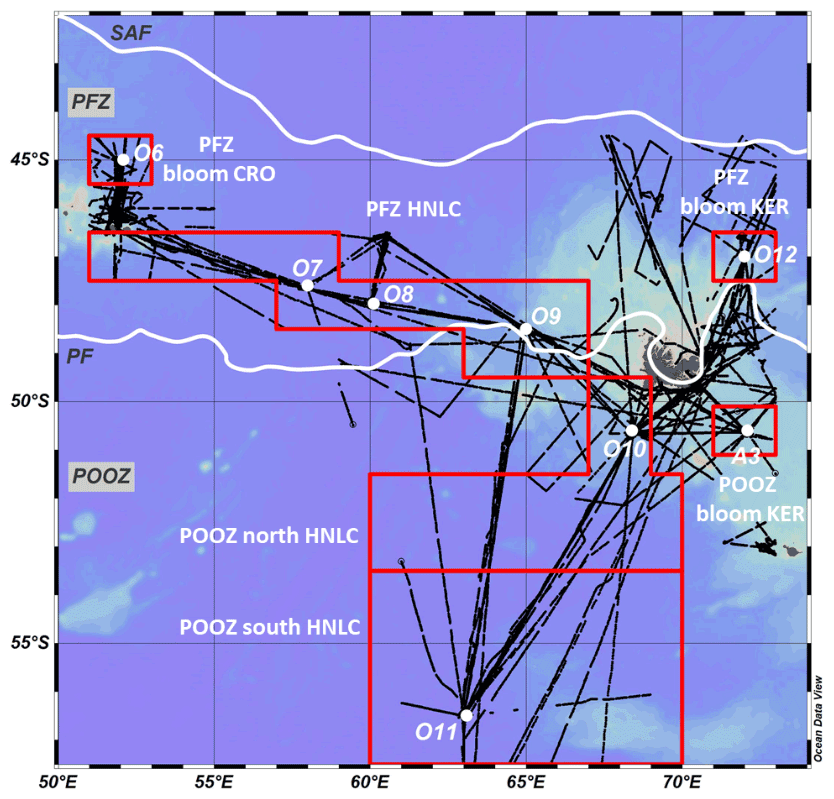
Figure 2 Tracks of summer cruises in 1998–2019 with sea surface fCO₂ data (black dots) from SOCAT version v2020 (Bakker et al., 2020). The six areas identified in Tables 2–4 are represented with red square boxes. SAF and PF are indicated in white as in Fig. 1. PFZ stands for polar front zone and POOZ for permanent open-ocean zone (i.e. north of the winter ice edge). Bathymetry is plotted as background based on GEBCO-2019 (figure produced with ODV; Schlitzer, 2021).

To investigate the decadal fCO₂ and pH trends we thus separate the domain in six main sectors (Fig. 2): (i) HNLC waters in the polar front zone (PFZ) between the SAF and the PF and (ii) north and (iii) south parts of HNLC waters south of the PF in the permanent open-ocean zone (POOZ), as well as the phytoplanktonic bloom regions associated with (iv) the Crozet shelf and (v) the north and (vi) the south of Kerguelen shelf.

The HNLC waters in the POOZ have been divided into northern and southern parts because the two stations in this region are very distant (O10: 50.6^∘ S; O11: 56.6^∘ S; Fig. 1). Station O10 is at the edge of the continental shelf of Kerguelen (bottom depth 1650 m) and was occupied more often than Station O11 in the open ocean (bottom depth 4850 m).

2.2 Data collection and measurements

This study is based on observations collected in the framework of the French long-term monitoring programme OISO (Océan Indien Service d'Observation) initiated in 1998. During these OISO cruises, both sea surface underway and water-column measurements are collected. Data in the water column were collected using a CTD sensor (conductivity–temperature–depth) coupled to an oxygen (O₂) sensor and a fluorimeter and equipped with twenty-four 12 L Niskin bottles to sample for A_T, C_T, O₂, nutrients and chlorophyll a (chl a). In addition, surface samples were collected every 4 to 8 h for salinity, nutrients and chl a. Analytical methods for these cruises followed the protocols used since 1998 described previously (e.g. Metzl et al., 2006; Metzl, 2009; Mahieu et al., 2020; Lo Monaco et al., 2021).

Temperature and salinity were measured using a SeaBird thermosalinograph (SBE 45) for surface data and a SeaBird CTD (SBE911+) for water-column profiles. A control of the CTD data, and in some cases an adjustment, is done using the discrete salinity samples analysed at LOCEAN (Laboratoire d'Océanographie et du Climat: Expérimentation et Approches Numériques) using a Guildline Autosal or Portasal salinometer and using IAPSO standards provided by Ocean Scientific International Ltd (OSIL). Accuracies of temperature and salinity are, respectively, 0.005 ^∘C and 0.01. The O₂ sensor data were also checked against measurements of samples collected from the Niskin bottles and analysed on board following the Winkler method (Carpenter, 1965) using a METTLER titrator and iodate standards provided by OSIL.

A_T and C_T were semi-continuously (3 to 4 samples per hour) measured in surface waters using a potentiometric titration method (Edmond, 1970) in a closed cell. The same method is used (on board) to analyse the samples collected in the water column. The repeatability for A_T and C_T based on the analysis of duplicates (in surface waters and around 1000 m or in bottom waters) varies from 1.0 to 3.5 µmol kg⁻¹. The accuracy of A_T and C_T measurements (always better than ± 3.0 µmol kg⁻¹ for all cruises since 1998) was ensured by daily analyses of certified reference materials (CRMs) provided by the A. G. Dickson laboratory (Scripps Institute of Oceanography).

For fCO₂ measurements, sea surface water was continuously equilibrated with a “thin-film-type” equilibrator thermostated with surface seawater (Poisson et al., 1993). The CO₂ in the dried gas was measured with a non-dispersive infrared analyser (NDIR; Siemens ULTRAMAT 5F or 6F). Standard gases for calibration (around 270, 350 and 480 ppm and certified at LSCE, Laboratoire des Sciences du Climat et de l'Environnement) were measured every 5 to 7 h. To correct the CO₂ molar fraction (xCO₂) dry measurements to fCO₂ in situ data, we used polynomials given by Weiss and Price (1980) for vapour pressure and by Copin-Montegut (1988, 1989) for temperature.

For nutrients (nitrite, nitrate, silicate and, for some years, phosphate), samples were filtered (at 0.2 µm) and either poisoned with HgCl₂ and kept cold (for nitrite, nitrate and silicate) or frozen at −80 ^∘C (for phosphate). Nitrite, nitrate and silicate were analysed on board or at LOCEAN by colorimetry using an auto-analyser (Bran + Luebbe) according to the method of Tréguer and Le Corre (1975) until 2009, then following the method of Coverly et al. (2009). The uncertainty of these measurements is on the order of ± 0.1 µmol kg⁻¹. Phosphate samples (for some cruises) were analysed using a spectrometer according to the method of Murphy and Riley (1962) and revised by Strickland and Parsons (1972), with an uncertainty of ± 0.02 µmol kg⁻¹.

For the water-column data obtained between 1998 and 2011 secondary quality controls were performed in the frame of the CARINA (Carbon Dioxide in the Atlantic Ocean) and GLODAP-v2 (Global Ocean Data Analysis Project version 2) projects (Lo Monaco et al., 2010; Key et al., 2015; Olsen et al., 2016). For OISO cruises conducted since 2012 (not yet included in GLODAP-v2) we proceeded to a data quality control following the same protocol as for GLODAP-v2 (comparison with deep waters), and we found no systematic bias for the properties measured during these cruises as described in detail by Mahieu et al. (2020). All the data (and metadata) will be delivered to OCADS (Ocean Carbon and Acidification Data System) NCEI (National Centers for Environmental Information) database and to GLODAP-v2-2023.

The surface underway fCO₂, A_T and C_T data (and metadata) are available at the NCEI/OCADS database (http://www.ncei.noaa.gov/access/ocean-carbon-data-system/oceans/VOS_Program/OISO.html, last access: 30 April 2020). The oceanic fCO₂ data are also available in the SOCAT data product (Bakker et al., 2016). Note that all the data used come from fCO₂ measurements from OISO cruises, except one in 2004/2005 near Crozet Island (expocode 74E320041213 in SOCAT). Note also that when added to SOCAT, original fCO₂ data are recomputed (Pfeil et al., 2013) using the temperature correction from Takahashi et al. (1993). Given the small difference between sea surface temperature (SST) and equilibrium temperature, the fCO₂ data from our cruises are identical (within 1.0 µatm) in SOCAT and NCEI/OCADS. Here we used fCO₂ values as provided by SOCAT.

2.3 Data selection

To investigate the fCO₂ and pH trends and their drivers over the period 1998–2019 we used the observations regularly conducted during summer cruises (one summer cruise per year, between December and beginning of March). The sea surface fCO₂ and pH trends were evaluated using three datasets: (i) underway temperature, salinity and fCO₂ data, (ii) underway temperature, salinity, A_T and C_T data, and (iii) temperature, salinity, A_T and C_T data averaged in the summer mixed layer at each station representative of each domain (Figs. 1 and 2).

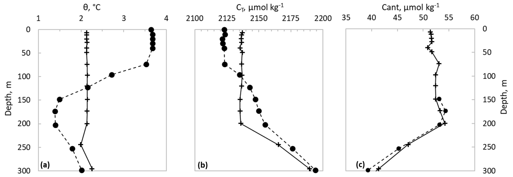
Figure 3 Vertical profiles of (a) potential temperature, (b) C_T and (c) C_ant (TrOCA method) for two seasons: during winter (July 2000, cross) and summer (January 2001, circle) at Station O10. The C_ant concentrations for each year were estimated just below the summer mixed layer. Note that C_ant during summer in the upper layer is uncertain (results not shown) but below 125 m C_ant in summer should correspond to C_ant in winter.

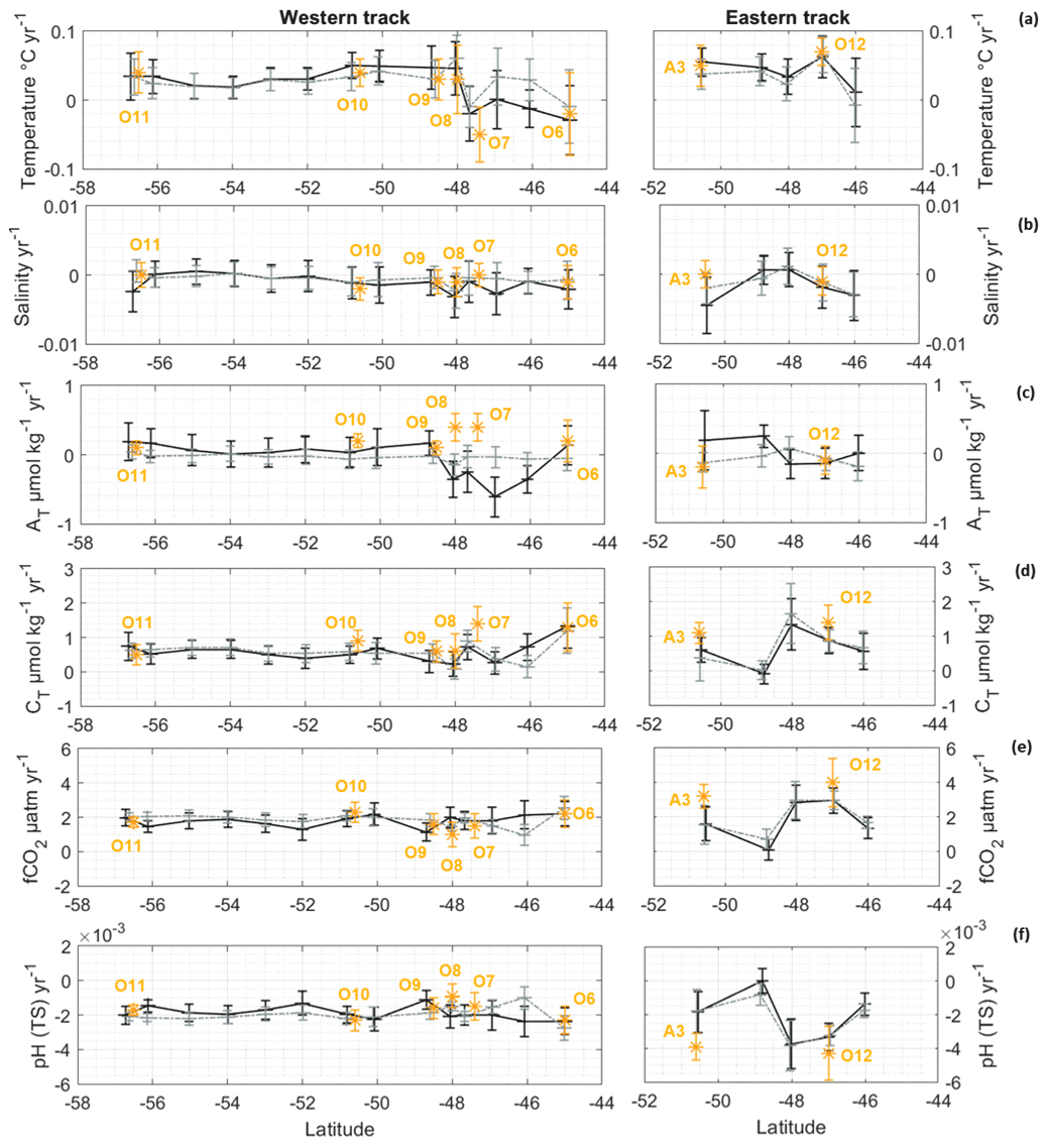
Figure 4 Trends (per year) of temperature (a), salinity (b), A_T (c), C_T (d), fCO₂ (e) and pH (f) evaluated from the fCO₂ surface dataset (in grey), the A_T and C_T surface dataset (in black), and the A_T and C_T data in the mixed layer at each station (in orange) along the western and eastern tracks (see Fig. S4 in the Supplement). The computation method is explained in the Sect. 2.3.

In order to estimate the trends from underway datasets, gridded values for each cruise were averaged in boxes of 1^∘ of latitude and 2^∘ of longitude. Some boxes were enlarged if the surrounding boxes were homogeneous for both physical and biogeochemical parameters. Then, trends were estimated provided some conditions were fulfilled (as on Fig. 4): the box must contain at least eight cruises (years) and must have been visited at the beginning of the period in at least one of the years of 1998, 1999 and 2000, as well at the end of the period, in at least one of the years of 2017, 2018 and 2019. Finally, the boxes were grouped into six large regions (Fig. 2). As we are interested in separating the anthropogenic signal from natural variability for both fCO₂ and pH trends, and because anthropogenic CO₂ concentrations are not well evaluated in surface waters, we also estimated the trends at each station selecting the data just below the summer mixed layer (a layer referred to as BML). South of the PF, this subsurface layer corresponds to the winter water clearly identified by a subsurface temperature minimum observed in summer at 150–200 m (Fig. 3; Metzl et al., 2006; Mackay and Watson, 2021).

From the station dataset, the mixed layer was defined for each station and each year. To evaluate the depth of the mixed layer, we carefully looked at profiles for each station and each period and identified the layer where properties are homogeneous (including O₂, nutrients, A_T and C_T). On average the summer mixed layer depth over the period 1998–2019 is between 50 and 75 m for the PFZ region (stations O6–O9 and O12) and between 75 and 100 m for the POOZ region (stations A3, O10 and O11). Results for each station in the mixed layer will then be compared to those obtained in the corresponding boxes and regions.

2.4 Calculations of the carbonate system parameters and contributions

Any parameter of the carbonate system can be computed from two other carbonate system parameters, together with temperature, salinity, silicate and phosphate data. In this study, we compared the measured fCO₂ to fCO₂ calculated from A_T and C_T, as well as pH calculated either from A_T and C_T or from fCO₂ and A_T (reconstructed from salinity, see below). When nutrient data were missing (notably phosphate that was not measured during all cruises), we used monthly climatological values derived from the OISO data available over the period 1998–2019. Because nutrient interannual variability is low, this choice does not impact the carbonate system parameter calculations. The calculation programme used is CO₂SYS originally developed by Lewis et al. (1998). We used the MATLAB version (van Heuven et al., 2011) that now includes error propagation (Orr et al., 2018). The constants of thermodynamic equilibrium of CO₂ in seawater used are K₁ (for the dissociation of carbonic acid) and K₂ (for the bicarbonate ion) defined by Mehrbach et al. (1973) and refitted by Dickson and Millero (1987). The total boron value is calculated according to Uppström (1974), and the KHSO₄ dissociation constant is from Dickson (1990). The adopted pH scale is total scale. When A_T data were not available, it was estimated from salinity. The correlation between sea surface A_T and salinity in the open ocean is modelled with an empirical linear relationship (Millero et al., 1998; Friis et al., 2003). Here we used the A_T–S relationship estimated from the OISO data (underway A_T and C_T dataset) over the period 1998–2019 (summer cruises; Eq. 1).

$$\begin{array}{}\text{(1)}& A_{\mathrm{T}}=\mathrm{64.341}\times S+\mathrm{106.764}\end{array}$$

(RMSE = 7.485 µmol kg⁻¹, r² = 0.41, n = 4775).

In order to quantify the accumulation of anthropogenic carbon (C_ant) below the mixed layer, two methods were used: the TrOCA method (Traceur combinant Oxygène, Carbone et Alcalinité), developed by Touratier and Goyer (2004) and refitted by Touratier et al. (2007), and the preformed carbon method (C⁰), independently developed by Brewer (1978) and Chen and Millero (1979), using the parameterisations from Lo Monaco et al. (2005b) for the Indian sector of the Southern Ocean.

The method of Touratier and Goyet (2004) is based on the quasi-conservative tracer TrOCA defined according to Eq. (2). The tracer TrOCA contains information on both the origin of water masses and the invasion of anthropogenic carbon. Touratier and Goyet (2004) showed that for a given year, there is a relationship between the distribution of TrOCA in the ocean and potential temperature (θ). Touratier et al. (2007) improved the relationship by adding A_T in the formulation. Using data collected in old deep water (free from anthropogenic carbon), they proposed an empirical relationship to predict the pre-industrial value of TrOCA (TrOCA⁰ in Eq. 3). The accumulation of C_ant (Eq. 4) can be inferred from the increase in TrOCA since the pre-industrial era. The coefficients used in Eqs. (2)–(4) are as follows: a = 1.279; b = 7.511; c = −1.087 × 10⁻²; d = −7.81 × 10⁵ (Touratier et al., 2007).

$$\begin{array}{}\text{(2)}& {\displaystyle }& {\displaystyle }\mathrm{TrOCA}={\mathrm{O}}_{\mathrm{2}}+a(C_{\mathrm{T}}-\mathrm{0.5}{A}_{\mathrm{T}})\text{(3)}& {\displaystyle }& {\displaystyle }{\mathrm{TrOCA}}^{\mathrm{0}}=\exp \left\{b+\left(c\mathit{\theta }\right)+\left({\displaystyle \frac{d}{A_{\mathrm{T}}^{\mathrm{2}}}}\right)\right\}\text{(4)}& {\displaystyle }& {\displaystyle }{C}_{\mathrm{ant}}^{\mathrm{TrOCA}}={\displaystyle \frac{\mathrm{TrOCA}-{\mathrm{TrOCA}}^{\mathrm{0}}}{a}}\end{array}$$

The C⁰ method is a back-calculation technique that evaluates the preformed carbon concentration (concentration at the surface at the time of water mass formation, C^0,t) and its pre-industrial component. Indeed, C^0,t (that can be estimated by removing the inorganic carbon generated in situ by biological processes, C_bio) is composed of a pre-industrial part (C^0,PI) and an anthropogenic part (C_ant) resulting from the uptake of anthropogenic CO₂ from the atmosphere. Thus, anthropogenic carbon in the ocean interior can be calculated from C_T measurements by correcting for its natural components (C_bio and C^0,PI) according to Eq. (5). The pre-industrial component will not be discussed here because, as a time constant, it does not contribute to the evolution of C_ant (refer to the study by Lo Monaco et al., 2005b). The biological contribution is the carbon added by carbonate dissolution (C_carb) and the remineralisation of the soft tissue (C_soft). It can be determined from measurements of A_T, O₂, and the molar ratios $\frac{\mathrm{C}}{{\mathrm{O}}_{\mathrm{2}}}$ and $\frac{\mathrm{N}}{{\mathrm{O}}_{\mathrm{2}}}$ (here we used the ratio determined by Körtzinger et al., 2001), according to Eqs. (6)–(8).

$$\begin{array}{}\text{(5)}& {\displaystyle }& {\displaystyle }{C}_{{\mathrm{ant}}^{\mathrm{0}}}=C^{\mathrm{0},t}-C^{\mathrm{0},\mathrm{PI}}=C_{\mathrm{T}}-C_{\mathrm{bio}}-C^{\mathrm{0},\mathrm{PI}}\text{(6)}& {\displaystyle }& {\displaystyle }{C}_{\mathrm{bio}}=C_{\mathrm{carb}}+C_{\mathrm{soft}}\text{(7)}& {\displaystyle }& {\displaystyle }{C}_{\mathrm{carb}}=\mathrm{0.5}\left\{\left(A_{\mathrm{T}}-A_{\mathrm{T}}^{\mathrm{0}}\right)-\left({\displaystyle \frac{\mathrm{N}}{{\mathrm{O}}_{\mathrm{2}}}}\text{AOU}\right)\right\}\text{(8)}& {\displaystyle }& {\displaystyle }{C}_{\mathrm{soft}}=-{\displaystyle \frac{\mathrm{C}}{{\mathrm{O}}_{\mathrm{2}}}}\text{AOU}\end{array}$$

Two other terms are introduced into Eqs. (7) and (8): preformed A_T ($A_{\mathrm{T}}^{\mathrm{0}}$) and apparent oxygen utilisation (AOU). $A_{\mathrm{T}}^{\mathrm{0}}$ is derived from a multiparametric relationship observed in surface water in winter (at the time of water mass formation). Studies have shown that A_T in surface waters varies in relation to oceanic tracers such as temperature, salinity and nutrients (Poisson and Chen, 1987; Körtzinger et al., 1998). It is possible to estimate $A_{\mathrm{T}}^{\mathrm{0}}$ by assuming that the relationship between A_T and other oceanic tracers has remained the same since the pre-industrial era. This assumption is supported by observations (see “Results” section). Furthermore, since the air–sea exchange of oxygen is rapid and winter mixed layers are not too deep, winter O₂ concentrations in surface waters are close to equilibrium with the atmosphere (except in areas covered with sea ice). We thus assume that the preformed oxygen corresponds to oxygen saturation (${\mathrm{O}}_{\mathrm{2}}^{\mathrm{sat}}$). The term AOU is thus introduced and defined as the difference between oxygen saturation (which depends on the temperature of the water; Benson and Krause, 1980) and the measured oxygen (AOU = ${\mathrm{O}}_{\mathrm{2}}^{\mathrm{sat}}$ − O₂).

The trends in fCO₂ and pH can be driven by changes in temperature, salinity, A_T and/or C_T (e.g. Keeling et al., 2004; Munro et al., 2015; Leseurre et al., 2020). For C_T, this includes the contribution of C_ant and the natural component (C_T = C_ant + C_nat). The contribution of each driver is evaluated by allowing a change in only one parameter according to their observed trend while setting the other parameters to their mean values (Eq. 9). The uncertainty of the contribution was evaluated by performing 1000 random perturbations within the range of the standard deviation of the observed trends in temperature, salinity, A_T and C_T.

$$\begin{array}{}\text{(9)}& {\displaystyle \frac{\mathrm{d}X}{\mathrm{d}t}}={\displaystyle \frac{\partial X}{\partial T}}{\displaystyle \frac{\mathrm{d}T}{\mathrm{d}t}}+{\displaystyle \frac{\partial X}{\partial S}}{\displaystyle \frac{\mathrm{d}S}{\mathrm{d}t}}+{\displaystyle \frac{\partial X}{\partial A_{\mathrm{T}}}}{\displaystyle \frac{\mathrm{d}{A}_{\mathrm{T}}}{\mathrm{d}t}}+{\displaystyle \frac{\partial X}{\partial C_{\mathrm{T}}}}{\displaystyle \frac{\mathrm{d}{C}_{\mathrm{T}}}{\mathrm{d}t}},\end{array}$$

where X corresponds to fCO₂ or pH.

We tested the impact of fresh water fluxes on A_T and C_T by normalising to a salinity of 34 (following the method of Munro et al. (2015) in the Drake Passage of the Southern Ocean). The contribution of A_T and C_T being very close to the ones of normalised A_T and C_T, we chose not to discuss these last ones in this paper.

3 Results

3.1 Decadal trends in surface waters

The trends in surface waters estimated using the three datasets are presented in Fig. 4 and listed in Tables 2–4. For clarity we separated the western and eastern tracks (west and east of 70^∘ E). As expected in the context of global warming, we observe a warming in surface waters south of 48^∘ S (+0.05 ^∘C yr⁻¹ on average; Fig. 4a, Tables 2–4); however, there is no significant change in salinity (Fig. 4b). Thus, A_T calculated from salinity (Eq. 1) does not present a decadal change, which is confirmed by A_T measurements (underway and station data) with the exception of a small area in the PFZ near 47–48^∘ S on the western track (Fig. 4c). In this area, underway A_T measurements suggest a slight decrease, whereas the mixed layer data (stations O7 and O8) suggest an increase in A_T of +0.4 µmol kg⁻¹ yr⁻¹ (Fig. 4c, Table 2). Note that at Station O7 we also observed an anomaly in the temperature trend (cooling; Fig. 4a) that may reflect small-scale variability (due to the intermittent presence of eddies or meanders).

The trends in C_T obtained from measured values (underway or station data) or calculated values (from fCO₂ observations) show a good agreement. Surface C_T concentrations increased in all regions (Fig. 4d) by +0.4 to +1.4 µmol kg⁻¹ yr⁻¹ (Tables 2–4). The C_T trends are rather homogeneous in the south (around +0.6 µmol kg⁻¹ yr⁻¹) and present more variability in the eastern region (near Kerguelen Island). As expected, the trend in fCO₂ is positive in all regions (from +1.0 to +4.0 µatm yr⁻¹; Fig. 4e, Tables 2–4), and it is generally very similar when using underway fCO₂ measurements or fCO₂ calculated with A_T–C_T pairs from both underway and mixed layer data. The same is true for the pH trend calculated from the three datasets: it is always negative (from −0.0014 to −0.0043 yr⁻¹; Fig. 4f, Tables 2–4) and generally in good agreement. As for temperature and C_T, the fCO₂ and pH trends are rather homogeneous south of 50^∘ S and more variable in the vicinity of Kerguelen Plateau (eastern track) where the variations in pH mirror those of fCO₂ and C_T.

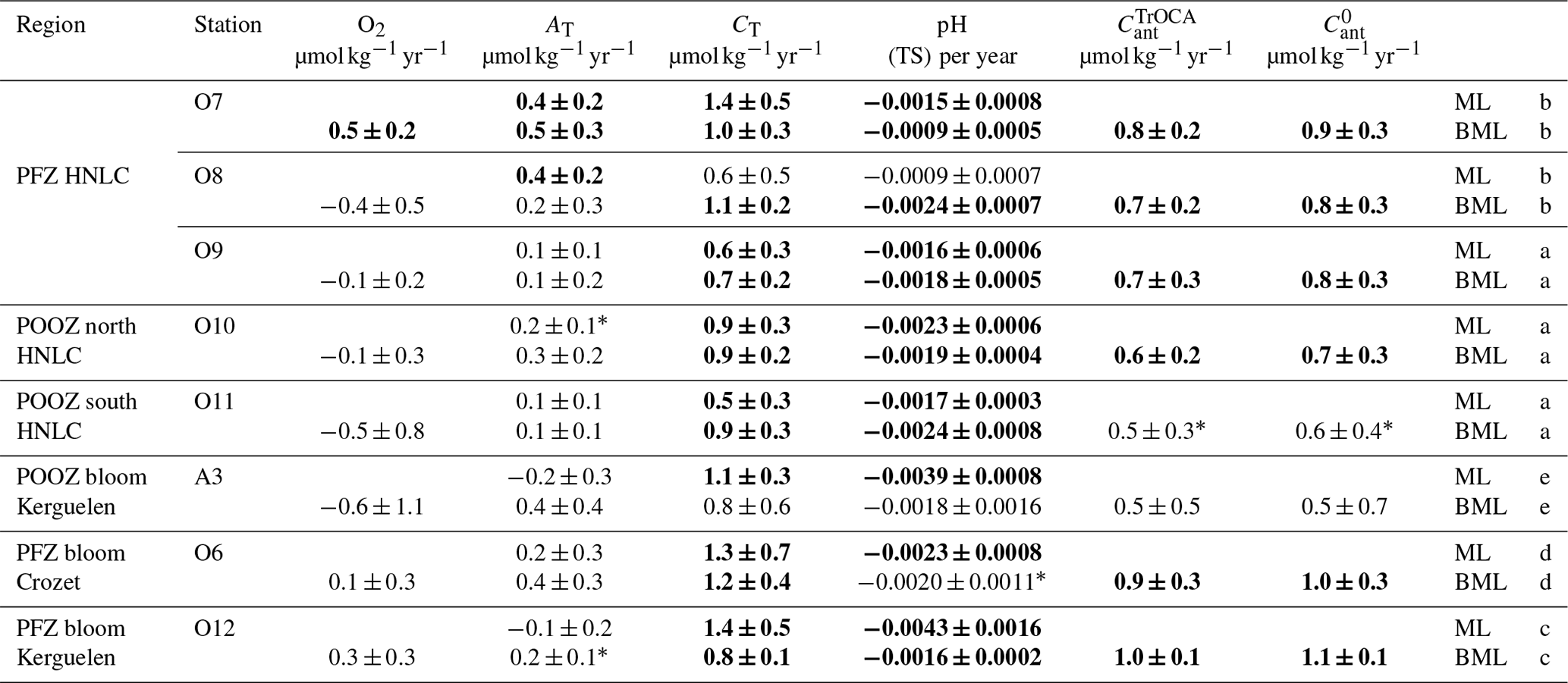
Table 1 Trends (per year) of O₂, A_T, C_T, pH (total scale, TS) and C_ant (TrOCA and C⁰ methods) evaluated from the A_T and C_T data in the summer mixed layer (ML) and below the summer mixed layer (BML) at each station between (a) 1998 and 2019, (b) 1998 and 2017, (c) 1999 and 2019, (d) 2000 and 2019, and (e) 2005 and 2019. C_ant is only estimated below the mixed layer (see Fig. 3). The significant trends (Student's t test) are represented in bold (at 95 %) or with a star (at 90 %).

The three datasets generally show similar changes, which indicates that the trends evaluated locally (in the mixed layer) are representative of the trends observed in wider areas (underway data). This does not hold in the Kerguelen bloom because stations O12 and A3 are generally in high production areas, while the underway data averaged in the boxes also include lower production areas (Fig. 1). In the next sections we will focus on the results from the mixed layer (stations) data that we grouped in three domains (PFZ HNLC, POOZ HNLC and bloom regions). We choose this dataset because it can be completed by subsurface data, allowing for the calculation of anthropogenic CO₂ (C_ant).

Figure 5 C_T trends in the summer mixed layer (ML) and below the summer mixed layer (BML). Decomposition of $C_T^{\mathrm{BML}}$ in C_ant (TrOCA and C⁰ methods) and C_bio from C⁰ method. The three phytoplanktonic bloom stations are reported in yellow (last three) and are separated from the HNLC stations (first five, shown in blue). To help the interpretation, a map with the localisation of these station is included (same map as Fig. 1).

3.2 Drivers of surface fCO₂ and pH trends

3.2.1 Accumulation of anthropogenic CO₂

To gain insight into the C_T, fCO₂ and pH trends, we separated the natural versus anthropogenic CO₂ contributions in subsurface water masses by selecting the data below the summer mixed layer (BML in Table 1). As described in Sect. 2, we used two methods to estimate C_ant. In the investigated domain south of the SAF we obtained C_ant concentrations ranging from 40 to 75 µmol kg⁻¹ for the TrOCA method and from 35 to 80 µmol kg⁻¹ for the C⁰ method. The difference in C_ant concentrations can be explained by uncertainties in the pre-industrial terms (TrOCA⁰, Eq. 3; C^0,PI, Eq. 5; e.g. Pardo et al., 2014). Since the pre-industrial terms should remain steady for a given water mass, the errors cancel out when estimating a change in C_ant, and therefore the two methods give very similar trends ranging from +0.5 to +1.1 µmol kg⁻¹ yr⁻¹ depending on the region (Table 1). In most regions, the C_ant trend is relatively close to the C_T trend calculated below the mixed layer (BML in Table 1, Fig. 5). Some small differences can be attributed to natural processes (e.g. change in biological activity or mixing) that need to be considered when interpreting the fCO₂ and pH trends. Our results also show a north–south gradient of C_ant trends (Table 1), with higher values at the two northernmost sites (+0.9 to +1.1 µmol kg⁻¹ yr⁻¹, stations O6 and O12), medium values farther south in the PFZ (+0.7 to +0.9 µmol kg⁻¹ yr⁻¹, stations O7–O9) and lower trends south of the PF (+0.5 to +0.7 µmol kg⁻¹ yr⁻¹, stations A3, O10 and O11).

Table 2 Trends (per year) evaluated in the HNLC part of PFZ, from the fCO₂ surface dataset, the A_T and C_T surface dataset and the A_T and C_T data in the mixed layer at each station (O7–O9), estimated between (a) 1998 and 2019 or (b) 1998 and 2017. The significant trends (Student's t test) are represented in bold (at 95 %) or with a star (at 90 %).

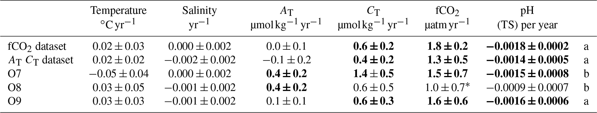
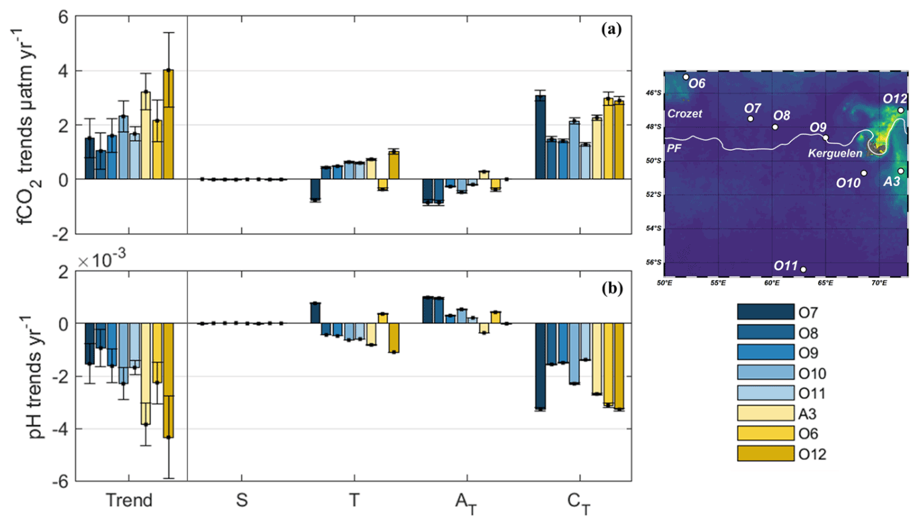
Figure 6 Trends and decomposition of fCO₂ (a) and pH (b) in the summer mixed layer, according to Eq. (9). The effect of change in salinity (S), temperature (T), A_T and C_T is shown. The three phytoplanktonic bloom stations are reported in yellow (last three) and are separated from the HNLC stations (first five, shown in blue). To help the interpretation, a map with the localisation of these station is included (same map as Fig. 1).

3.2.2 The polar front zone

Data collected in the PFZ between Crozet and Kerguelen islands (stations O7–O9) show a surface fCO₂ increase between +1.0 and +1.6 µatm yr⁻¹ and a pH decrease between −0.0009 and −0.0016 yr⁻¹ (Table 2). At stations O7 and O9 the fCO₂ and pH trends in the mixed layer are similar (around +1.5 µatm yr⁻¹ and −0.0015 yr⁻¹) and coherent with those derived from underway fCO₂ or A_T–C_T observations averaged in the PFZ HNLC domain. However, the processes that explain these trends are different. At Station O7, the rapid increase in C_T (+1.4 µmol kg⁻¹ yr⁻¹) is countered by an increase in A_T (+0.4 µmol kg⁻¹ yr⁻¹) and the cooling of surface waters (Fig. 6a and b). A very similar increase in A_T is observed below the mixed layer, while the C_T trend is slightly lower and mainly explained by the accumulation of C_ant (Table 1). The small difference between the surface and subsurface C_T trends of +0.4 µmol kg⁻¹ yr⁻¹ at Station O7 could be due to a larger accumulation of C_ant or higher natural variability at the surface. In contrast, at Station O9 the C_T trends are the same in surface and subsurface waters and identical to the C_ant trend below the mixed layer (all around +0.7 µmol kg⁻¹ yr⁻¹). At this station we did not observe a significant trend in temperature or A_T, and thus surface fCO₂ and pH trends are solely attributed to the accumulation of C_ant (Figs. 5 and 6). Finally, Station O8 shows a mixed scenario: the surface C_T trend is as low as for Station O9 (around +0.6 µmol kg⁻¹ yr⁻¹) and could be mainly explained by the accumulation of C_ant, but the trends in surface fCO₂ and pH are also affected by an increase in A_T (like for Station O7). Note that at Station O8 the C_T trend observed below the mixed layer could result from both anthropogenic and natural processes, as suggested by the decrease in oxygen (although not significant, not shown) that could reflect an increase in organic matter remineralisation (significant contribution of C_bio in Fig. 5).

Table 3 Trends (per year) evaluated in the HNLC part of (1) the north and (2) the south POOZ, from the fCO₂ surface dataset, the A_T and C_T surface dataset, and the A_T and C_T data in the mixed layer at each station (O10 and O11), estimated between (a) 1998 and 2019. The significant trends (Student's t test) are represented in bold (at 95 %) or with a star (at 90 %).

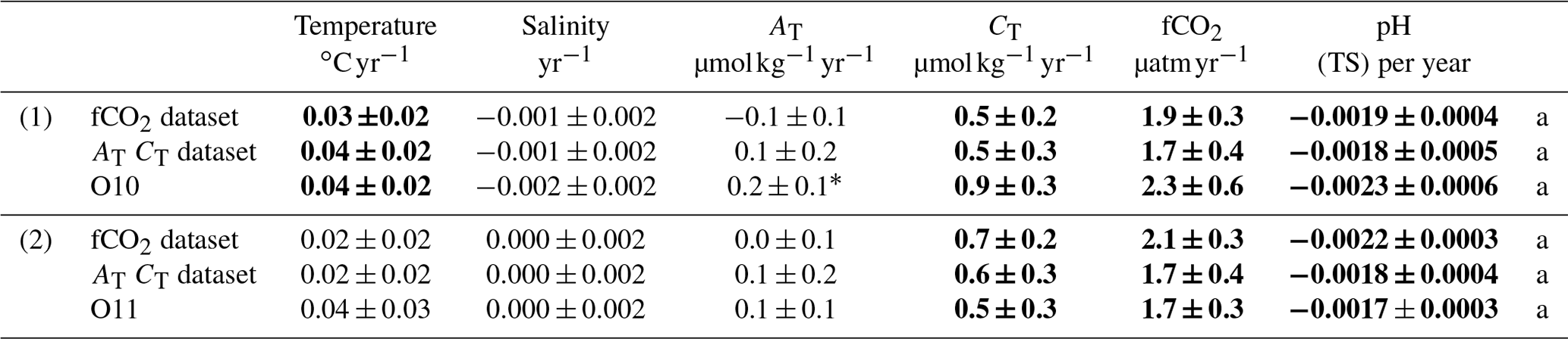
3.2.3 The POOZ HNLC

South of the polar front in the POOZ HNLC waters we found similar results at the northern station (O10 around 50^∘ S) and southern station (O11 at 56^∘ S) (Figs. 5 and 6). In this large domain, the surface fCO₂ increase (between +1.7 and +2.3 µatm yr⁻¹) and pH decrease (between −0.0017 and −0.0023 yr⁻¹) are mainly explained by the C_T increase (between +0.5 and +0.9 µmol kg⁻¹ yr⁻¹) and, to a lesser extent, by the sea surface warming (up to +0.04 ^∘C yr⁻¹) (Table 3, Fig. 6). In this region we detect only a small increase in A_T at Station O10 (+0.2 µmol kg⁻¹ yr⁻¹; Table 3). Results obtained below the mixed layer at both stations suggest that the C_T change (+0.9 µmol kg⁻¹ yr⁻¹) can be mainly explained by the accumulation of C_ant (between +0.5 and +0.7 µmol kg⁻¹ yr⁻¹; Table 1), but other processes (or residuals of about 30 %) also contribute to the trend (Fig. 5).

Table 4 Trends (per year) evaluated in the phytoplanktonic bloom of (1) Crozet in the PFZ and of Kerguelen in the (2) PFZ and (3) POOZ, from the fCO₂ surface dataset, the A_T and C_T surface dataset, and the A_T and C_T data in the mixed layer at each station (O6, O12 and A3), estimated between (c) 1999 and 2019, (d) 2000 and 2019, and (e) 2005 and 2019. The significant trends (Student's t test) are represented in bold (at 95 %) or with a star (at 90 %).

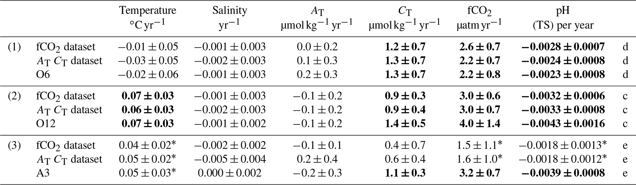
3.2.4 Phytoplanktonic blooms near Crozet and Kerguelen islands

In the phytoplanktonic bloom regions near Crozet and Kerguelen islands, fCO₂ increased and pH decreased faster than in the corresponding HNLC waters (PFZ or POOZ; Table 4, Fig. 4e and f). North of Crozet Island (Station O6, in the PFZ), the increase in fCO₂ (+2.2 ± 0.8 µatm yr⁻¹) and decrease in pH (−0.0023 ± 0.0008 yr⁻¹) are mainly driven by a rapid increase in C_T (+1.3 ± 0.7 µmol kg⁻¹ yr⁻¹; Table 4, Fig. 6). A similar C_T trend is found below the mixed layer (Table 1) and is mainly explained by the increase in C_ant (around +0.9 or +1.0 µmol kg⁻¹ yr⁻¹; Table 1, Fig. 5). The fastest trends of fCO₂ and pH are found around Kerguelen Island at Station O12 in the PFZ (+4.0 ± 1.4 µatm yr⁻¹ and −0.0043 ± 0.0016 yr⁻¹) and Station A3 in the POOZ (+3.2 ± 0.7 µatm yr⁻¹ and −0.0039 ± 0.0008 yr⁻¹; Table 4). These trends result from both a significant warming (up to +0.07 ± 0.03 ^∘C yr⁻¹) and a rapid increase in C_T (up to +1.4 ± 0.5 µmol kg⁻¹ yr⁻¹; Table 4, Fig. 6). The C_T trend is slightly lower below the mixed layer at Station O12 (+0.8 ± 0.1 µmol kg⁻¹ yr⁻¹; Table 1) and is mainly explained by the accumulation of C_ant (Table 1, Fig. 5). Our data also show an increase in oxygen below the mixed layer at Station O12 (not shown) suggesting a decrease in organic matter remineralisation that could be partly compensated for by an increase in carbonate dissolution (increase in A_T; Table 1), leading to a small negative contribution of C_bio (Fig. 5). Note that at Station A3, repeated sampling started in 2005, and the trends were thus estimated for a shorter period (2005–2019) with fewer data collected in the water column than underway. This probably explains why the C_T, C_ant and pH trends are not significant below the mixed layer (Table 1, large uncertainty in C_ant compared to the other stations).

4 Discussion

4.1 Accumulation of anthropogenic CO₂

Our C_ant calculations based on subsurface data and two different methods show an increase between +0.5 and +1.1 µmol kg⁻¹ yr⁻¹, which suggests that most of the trends in surface C_T, fCO₂ and pH could be explained by the uptake of anthropogenic CO₂ by the ocean. In the region 40–60^∘ S, the C_T increase expected from equilibration with rising atmospheric CO₂ (+2.1 µatm yr⁻¹) would range from +0.8 to +1.2 µmol kg⁻¹ yr⁻¹ (theoretical C_T trend calculated at constant A_T, temperature and salinity). This range is due to the north–south variation in the $C_{\mathrm{T}}/A_{\mathrm{T}}$ ratio (or Revelle factor) from 0.88 at 45^∘ S to 0.94 at 60^∘ S (from 10 to 15 for the Revelle factor) based on our A_T–C_T observations. We thus expect to observe lower C_ant trends to the south (where the $C_{\mathrm{T}}/A_{\mathrm{T}}$ ratio is higher), which is in very good agreement with our results (Table 1). Such contrasting C_ant trends in the upper ocean north and south of the PF seem to be a permanent feature in the Southern Ocean (e.g. McNeil et al., 2001; Sabine et al., 2008; Tanhua et al., 2017; Gruber et al., 2019a, b). This latitudinal contrast is coherent with the C_ant change in the upper layer, estimated at the global scale by Gruber et al. (2019a) between 1994 and 2007. In the southern Indian sector, they estimated a mean C_ant accumulation of +10.7 (± 1.0) µmol kg⁻¹ in the band 45–50^∘ S and +6.0 (± 1.1) µmol kg⁻¹ in the band 50–55^∘ S south of the PF. This corresponds to a trend of +0.8 µmol kg⁻¹ yr⁻¹ in the north and of +0.5 µmol kg⁻¹ yr⁻¹ in the south, in good agreement with our results in the PFZ and POOZ (Table 1). Notice that this is an independent comparison as Gruber et al. (2019a, b) did not use the data presented here because their diagnostic approach requires phosphate data in the water column that were not measured during our cruises in 1998–2007. Our results also suggest higher C_ant trends in the PFZ at the two northernmost stations (+0.9 to +1.1 µmol kg⁻¹ yr⁻¹). Tanhua et al. (2017) also evaluated pronounced C_T changes (up to +1.2 µmol kg⁻¹ yr⁻¹) in subsurface waters of the PFZ from observations conducted in the South Atlantic (at about 0–10^∘ E) between 1990 and 2012. Note that the increase in C_ant in the POOZ is expected to become slower and slower as the Revelle factor increases slightly over time (by about +0.025 yr⁻¹ from 1998 to 2019 in the POOZ), which would reduce the CO₂ uptake by the ocean. However, the upwelling of C_T-rich but C_ant-poor deep waters is also an important process to consider as it controls both the relatively low C_ant concentrations estimated below the mixed layer south of the PF (e.g. Lo Monaco et al., 2005a; Pardo et al., 2014) and the uptake of CO₂ from the atmosphere (e.g. Le Quéré et al., 2007; Metzl, 2009).

4.2 Trends and drivers in the POOZ

Although the C_ant trends are smaller in the POOZ, the fCO₂ and pH trends in surface waters are slightly higher there than those observed in HNLC waters of the PFZ. This is because in the POOZ the fCO₂ and pH trends are driven by both C_ant (accounting for about 75 %) and the warming in surface waters (25 %). The warming in the POOZ over 1998–2019 deduced from our summer data both at the surface and in the mixed layer (between +0.02 and +0.05 ^∘C yr⁻¹) agrees with SST decadal trends derived at large scale in the Southern Ocean (e.g. Freeman and Lovenduski, 2015, for summer over 1998–2014; Auger et al., 2021, for summer over 1993–2017). In agreement with Auger et al. (2021), our data also indicate a pronounced sea surface warming around Kerguelen Island (between +0.04 and +0.07 ^∘C yr⁻¹).

Our data also suggest that in the POOZ HNLC region biological processes did not contribute to the decadal trend of oceanic fCO₂ and C_T. This is supported by low trends of surface chl a concentrations derived from remote sensing data over 1998–2012 (Gregg and Rousseaux, 2014) and confirmed after 2012 (result not shown). We note, however, that biological processes can have a large impact on fCO₂ and C_T at the interannual scale, which may bias the decadal trends.

4.2.1 Comparisons for the HNLC waters of the POOZ

Decadal fCO₂ trends (10 years or more) south of the PF deduced from (more or less) regular observations have been previously investigated in the Indian Ocean sector (Metzl, 2009; Xue et al., 2015), in the Atlantic Ocean sector at Drake Passage (Munro et al., 2015) and at large scale in the Southern Ocean (Takahashi et al., 2009; Lauvset et al., 2015; Table S1). Our results in the western Indian POOZ for the period 1998–2019 in summer (+2.1 ± 0.3 µatm yr⁻¹) are close to the fCO₂ trend deduced from winter data selected in the band 50–60^∘ S for the years 1986–2007 (+2.1 ± 0.6 µatm yr⁻¹; Takahashi et al., 2009), whereas Lauvset et al. (2015) estimated a lower fCO₂ trend in the Southern Ocean subpolar seasonally stratified (SO-SPSS) biome (+1.5 ± 0.1 µatm yr⁻¹ for 1991–2011). Xue et al. (2015) also estimated a much lower fCO₂ rate of +1.3 (± 0.4) µatm yr⁻¹ over 1993–2011 using summer observations in the eastern Indian sector, but these authors also noticed very contrasting trends when evaluated on shorter periods: +4.5 (± 1.0) µatm yr⁻¹ over 1993–1999 and +0.9 (± 0.5) µatm yr⁻¹ over 2000–2011. They attributed this change in the trend to the variation in the Southern Annular Mode (SAM) index happening around the year 2000, a direct link that we did not clearly detect in our observations. Our results in the Indian POOZ for summer are also higher than those observed in the Atlantic sector at Drake Passage over 2002–2015 (Munro et al., 2015) where the summer trend estimated south of the PF is +1.3 (± 0.9) µatm yr⁻¹. During winter, the fCO₂ trend of +0.7 (± 0.4) µatm yr⁻¹ south of the PF at Drake Passage over 2002–2015 (Munro et al., 2015) is more than 2 times lower than our estimate in the Indian POOZ when comparing data collected in August 2000 and June–July 2019 (+1.9 µatm yr⁻¹; Appendix A). Those fCO₂ trends in the Drake Passage have been revisited for the years 2002–2016 and extended to the SO-SPSS biome (Fay et al., 2018). In winter Fay et al. (2018) found a fCO₂ trend in the SO-SPSS of +1.8 (± 0.3) µatm yr⁻¹, close to our winter estimate, whereas in summer they found a fCO₂ trend of +1.2 (± 0.2) µatm yr⁻¹ much lower than in the atmosphere, suggesting that the carbon sink has been growing over 2002–2016 in the subpolar Southern Ocean (Fay et al., 2018). At first hand, this difference with our result is surprising as Fay et al. (2018) used the fCO₂ data from SOCAT version v5 that included the fCO₂ data from the OISO cruises in the southern Indian sector for the period 2002–2016. Interestingly, when selecting the same period as in Fay et al. (2018), we estimated a trend of +0.9 (± 0.2) µatm yr⁻¹ over 2002–2016 in the Indian POOZ, supporting the slow rates derived in the SO-SPSS biome for this period (Fay et al., 2018), as well as the rate observed over 2000–2011 in summer south of the PF in the eastern Indian sector (Xue et al., 2015). This highlights the sensitivity of the fCO₂ (or pH) trends to the period selected (and the start/end year pair), especially during summer (Fay and McKinley, 2013; Xue et al., 2015; Leseurre et al., 2020).

The averaged fCO₂ trend that we estimated over 1998–2019 in the POOZ (+2.1 ± 0.3 µatm yr⁻¹) is close to the trend in the atmosphere, suggesting that there is no significant deviation in CO₂ uptake for equilibration with the atmosphere in summer. This is opposite to a first analysis also based on fCO₂ data in the Indian POOZ but limited to the period 1991–2007 (Metzl, 2009), when the fCO₂ trend for summer was +2.4 (± 0.2) µatm yr⁻¹, leading to a reduction in the CO₂ sink. However, we found that in recent years oceanic fCO₂ increased at a much smaller rate (+0.3 ± 0.2 µatm yr⁻¹ over 2007–2019) compared to 1991–2007 (Metzl, 2009). In addition, when selecting the period 1998–2007, we estimated a much more rapid trend of +5.3 (± 0.4) µatm yr⁻¹ (Fig. S1 Station O11 in the Supplement), comparable to the trend observed in the eastern Indian sector in summer over 1993–1999 (Xue et al., 2015). This sensitivity of the fCO₂ trends to the period clearly visible in our data and previously reported in other sectors of the Southern Ocean (Xue et al., 2015; Fay et al., 2018) implies significant interannual to pluri-annual variations in the air–sea CO₂ fluxes in the Southern Ocean (e.g. Landschützer et al., 2015, 2016; Keppler and Landschützer, 2019).

The rapid fCO₂ increase in the Southern Ocean observed in the 1990s that implied a reduction of the carbon sink was interpreted as resulting from the intensification of the westerlies associated with a positive SAM index (probably driven by accelerating greenhouse gas emissions and stratospheric ozone depletion), which would have enhanced the upwelling of C_T-rich deep waters (e.g. Le Quéré et al., 2007; Lenton et al., 2009). Although ocean or coupled climate–carbon models suggest a close large-scale connection between the SAM and the carbon uptake in the Southern Ocean in the 1990s (Lenton and Matear, 2007; Le Quéré et al., 2007; Lovenduski et al., 2007; Lenton et al., 2009; Hauck et al., 2013; Gruber et al., 2019b), this does not hold for recent decades. Over 1990–2019, the mean annual SAM index remained mostly positive (except in 1996, 2002 and 2019), whereas the carbon sink in the Southern Ocean increased in the 2000s as opposed to the 1990s (Landschützer et al., 2015; Fay et al., 2018; Keppler and Landschützer, 2019). The link between the SAM and the fCO₂ trends (and air–sea CO₂ fluxes) at high latitudes based on regional observations over the last two or three decades is still an open question (Lenton et al., 2012; Ritter et al., 2017; Gregor et al., 2018; Keppler and Landschützer, 2019). The same holds for the pH trends that are closely linked to the fCO₂ trends. As opposed to observations in the eastern Indian sector (Xue et al., 2015, 2018), we did not identify in the POOZ a clear link between fCO₂ or pH variability and the SAM index for the period 1998–2019, a conclusion also deduced from the time-series data for the Drake Passage over 2002–2015 (Munro et al., 2015).

For pH our results in the HNLC POOZ over 1998–2019 in summer indicate a decrease ranging from −0.0017 to −0.0023 yr⁻¹. This is in the range of that deduced in the SO-SPSS biome over 1991–2011 (−0.0021 yr⁻¹; Lauvset et al., 2015), in the eastern Indian sector of the Southern Ocean for the period 1969–2003 (−0.0020 yr⁻¹; Midorikawa et al., 2012) and close to the trends observed over a shorter period of time in the southern Drake Passage in summer over 2002–2015 (−0.0017 yr⁻¹; Munro et al., 2015) or in the eastern Indian sector for the period 2001–2011 (−0.0016 yr⁻¹; Xue et al., 2018; Table S1). Once again, one should keep in mind that the trends are very sensitive to the period considered. Indeed, our time series in the southern POOZ highlights a rapid pH decrease over 1998–2005 (around −0.0050 ± 0.0016 yr⁻¹) and relatively stable pH values over 2010–2019 (Fig. S1 O11). This decadal change in the pH trend is directly linked to C_T and fCO₂ that also showed reduced trends in recent years in the POOZ. From our data we did not identify specific changes in the trends of other properties (e.g. temperature, salinity, A_T, oxygen or nutrients), and at that stage we had no clear explanation of the origin of the slowdown of the C_T, fCO₂ and pH trends in surface waters (e.g. change in circulation, mixing, biological processes).

Our results in HNLC waters of the Indian POOZ show significant pluri-annual variations in the CO₂ sink during summer that support previous studies conducted at the scale of the whole Southern Ocean (e.g. Landschützer et al. 2016), but our results only characterise the summer period, and one may wonder whether they also hold for the winter period. This issue was investigated using alternative data collected in our study region by a Saildrone USV (uncrewed surface vehicle) in June–July 2019 (Sutton et al., 2021) compared to OISO data collected in August 2000 (Appendix A).

4.2.2 Trends above Kerguelen Plateau south of the PF (Station A3)

Station A3 is located just south of the polar front above Kerguelen Plateau (Fig. 1) in a spring–summer bloom that occurs each year in this iron-fertilised area (Blain et al., 2007; Jouandet et al., 2008). An interesting result at this station is the fast trends derived in the mixed layer for C_T (+1.1 µmol kg⁻¹ yr⁻¹), fCO₂ (+3.2 µatm yr⁻¹) and pH (−0.0039 yr⁻¹) that are much higher than those obtained in HNLC waters (for example at Station O10 south-west of Kerguelen). It is worth remembering that fewer re-occupations were conducted at Station A3 since it was first sampled in 2005 (Fig. S1 A3), and, as this region presents high C_T, fCO₂ and pH variability in summer (both spatial and temporal) linked to the level and phasing of the phytoplankton bloom, the trends have larger uncertainties. For example, in late January 2014 and 2019 we observed relatively lower fCO₂ and C_T concentrations compared to the preceding years (Fig. S1 A3) that were linked to a more pronounced bloom during these periods. At that location, results from a multi-sensor mooring deployed from October 2016 to April 2017 showed high fCO₂ and C_T temporal variability in the surface layer (within 300–400 µatm and 2120–2160 µmol kg⁻¹ at 40 m; Pellichero et al., 2020). The underway surface fCO₂ data collected in this region in summer also presented very large spatial variability each year with gradients up to 100 µatm between data within and outside the bloom, as was first observed in January 1991 in this region (Poisson et al., 1993). Large spatial variability was also found in the underway C_T data in which differences of C_T within and out of the bloom can reach 30 µmol kg⁻¹ (Jouandet et al., 2008). At Station A3, the fCO₂, pH and C_T trends derived from the A_T–C_T data in the mixed layer are much stronger than those derived from surface underway data (Table 4). This is because we averaged the surface underway data in a grid square of 1^∘ × 1^∘ (the red box around Station A3 in Fig. 2), which somehow smooths the high spatial variability in most properties, whereas the mixed layer (station) data were all collected at the same position (but at different periods from mid-January to late-February). As an extreme case we compared the fCO₂ data in January 1991 (Poisson et al., 1993) with those obtained in January 2019 in the same region. Surprisingly, we observed almost the same fCO₂ values (Fig. S2 in the Supplement), although one would expect an increase of about +50 µatm over 28 years due to anthropogenic CO₂ uptake, not considering the warming of +0.7 ^∘C between 1991 and 2019. Thus, in January 2019 the region was a strong carbon sink reaching −100 µatm, whereas it was about −40 µatm in 1991. Again, this highlights the large interannual variations that are observed in summer in this bloom region and that limit the detection of the decadal trends in this region.

At Station A3, the data collected below the mixed layer (in the winter water) could partially reflect the properties of the surface layer during the preceding winter. Thus, our data may suggest lower trends in surface C_T and pH in winter than the rapid trends observed in summer in the surface mixed layer. However, this result is highly uncertain given the error associated with the trends derived below the mixed layer (Table 1). We have no direct observations in winter, but Station A3 was sampled in October 2005, 2011 and 2016 (pre-bloom periods before the summer stratification; e.g. Pellichero et al., 2020). Based on these three cruises we estimated an increase in fCO₂ of +2.2 (± 0.5) µatm yr⁻¹ (or +1.8 µatm yr⁻¹ when correcting for the observed warming of +0.05 ^∘C yr⁻¹) close to the atmospheric CO₂ increase. Using the A_T–S relationship (Eq. 1) and fCO₂ data in October 2005, 2011 and 2016, we estimated a C_T increase of +0.50 (± 0.15) µmol kg⁻¹ yr⁻¹, which is 2 times smaller than the trend obtained in summer from the mixed layer data but close to that deduced from the underway data (Table 4) and equal to the C_ant trend calculated below the mixed layer (Table 1). Results for pH calculated with fCO₂ data for October 2005, 2011 and 2016 lead to a decrease in pH with a rate of −0.0021 yr⁻¹ (± 0.0006), in better agreement with the values obtained in summer using underway data than using the station data (Table 4).

In conclusion, although there are large uncertainties about the fCO₂ and pH trends at Station A3 above the Kerguelen Plateau due to the variability in summer and the short time series (2005–2019), we believe that the rapid trends derived in the surface layer from the station data (in summer) are somehow real, but they result from a rapid increase in fCO₂ (decrease in pH) between 2007 and 2008 (detected in the station and underway datasets; Fig. S1 A3) that was followed by the stagnation of fCO₂ and pH values in recent years (according to the station dataset) or a reversal of the trends (according to the underway datasets). The reasons for such changes are still unknown, but this result highlights the need for pursuing this time series in order to properly predict the evolution of the carbonate system and the impact of ocean acidification in this region known as a biological hotspot.

4.3 Trends and drivers in the PFZ

For the PFZ lying between the SAF and the PF (Fig. 1), we separated the trend analysis in three domains: the HNLC zone between Crozet and Kerguelen islands (stations O7, O8 and O9) and the two northernmost stations located in fertilised waters north of Crozet (Station O6) and north of Kerguelen (Station O12).

4.3.1 Trends in the PFZ between Crozet and Kerguelen (stations O7–O9)

To estimate the trends of the properties at a regional scale in the PFZ HNLC waters we averaged the data along the repeated track between Crozet and Kerguelen islands (Fig. 2). In this domain, the fCO₂ and pH trends deduced from the underway and mixed layer (station) datasets appeared slightly lower than at higher latitudes (Fig. 4, Table 2). Because the C_ant trends are higher in the PFZ than in the POOZ, one would expect to observe higher fCO₂ and pH trends in the PFZ, but this is the opposite.

This region is influenced by the southern branch of the strong SAF current (observed in the band 43–47^∘ S) with a part deflected southward downstream of Crozet Island (Park et al., 1993). This circulation imprints zonal variability in surface properties and is most pronounced in the western part of the track around 55–58^∘ E where a signal of warmer water and lower fCO₂ was regularly observed in all seasons (Poisson et al., 1993). An example is shown for the OISO-14 cruise in January 2006 (Fig. S3 in the Supplement) showing low fCO₂ and C_T around 56–59^∘ E and higher concentrations east of 60^∘ E (this is also seen for nutrients, not shown). Such a zonal distribution motivated the repeated occupations of stations O7 and O8 located, respectively, at 58 and 60^∘ E: Station O7 was initially selected to reoccupy a historical station visited in 1978 and 1985 (GEOSECS and INDIGO-1 cruises) and to sample the intrusion of the warmer water from the north, while Station O8 aimed at sampling water in the PFZ less influenced by the southern branch of the SAF current. Station O9 is located on the western side of the Kerguelen archipelago and north of the Skiff Bank centred around 50^∘ S, 65^∘ E that rises up to 200 m below the surface (Fig. 2). This topographic feature controls the position of the PF that experiences seasonal and interannual variability in this region (Pauthenet et al., 2018). As opposed to stations O7 and O8, a temperature minimum (between 1.7 and 2.3 ^∘C) was observed almost each year around 200 m at Station O9 characterising the winter water and indicating that this location was very close to the PF at the boundary between the PFZ and the POOZ. Data from Station O9 were thus successfully selected to mimic C_T and fCO₂ distribution for austral winter in the Southern Ocean (Mackay and Watson, 2021).

The variability in the frontal system and currents in the PFZ between Crozet and Kerguelen islands imprints interannual changes in surface properties, which are more pronounced than in the POOZ. Note that for some years, not all three stations were visited (see Fig. S1 stations O7–O9), and the trends might be sensitive to the sampled years. For these reasons (frontal zone and sampling), we expected to observe some differences in the decadal change in surface properties, as well as in the drivers of fCO₂ and pH trends (Fig. 6). Indeed, at Station O7 we observed a cooling in surface waters not identified at stations O8 and O9 (Fig. 4a, Table 2) that actually occurred over a short period (2010–2017; see Fig. S1 O7). Over this short period, we also observed a rapid increase in C_T, which explains that the C_T trend in surface waters was also much higher at Station O7 than at stations O8 and O9 (Fig. 4d, Table 2). The surface underway data recorded near Station O7 (within the red box in Fig. 1) also showed a small cooling and higher C_T trend (Fig. S1 O7), supporting this signal. As cooling is also seen at depth at Station O7 (down to 300 m) we do not attribute this cooling to a change in air–sea heat fluxes. Instead, this is probably linked to the variability in the frontal system or of the meandering structure of the currents downstream of Crozet Island.

An intriguing result for stations O7 and O8 is the positive A_T trend observed in the mixed layer and below the mixed layer but not identified from underway A_T data and not observed at Station O9 (Tables 1 and 2). This A_T signal is not seen when reconstructing A_T from salinity, suggesting that it is biologically driven (e.g. presence of calcifying organisms; Balch et al., 2016) and that the A_T–S relationship is not always suitable to mimic the A_T distribution in this region. The impact of the A_T increase in the mixed layer is to decrease (increase) fCO₂ (pH), which opposes the effect of anthropogenic CO₂ uptake (Fig. 6a and b).

4.3.2 The phytoplanktonic bloom regions in the PFZ (stations O6 and O12)

Over the full period 1998–2019, the fastest fCO₂ and pH trends were observed at stations O6 and O12 located in the vicinity of Crozet and Kerguelen islands in phytoplanktonic bloom regions north of the PF (in the PFZ). As noted above, the C_ant trends at these northernmost stations are the highest (related to the $C_{\mathrm{T}}/A_{\mathrm{T}}$ ratio and possibly less mixing in winter with the C_ant-poor deep waters).

The Crozet bloom (Station O6)

Station O6 is located at 45^∘ S north of Crozet Island and south of the SAF and is close to or within the iron-fertilised phytoplankton bloom that occurs annually from September to January in this region (Planquette et al., 2007; Pollard et al., 2007; Venables et al., 2007; Sanial et al., 2014; Fig. 1). This bloom usually peaks in October, and therefore the biogeochemical data used in this study are the result of the biological processes that occurred a few months preceding the cruises. Thus, we could expect that the trends that we observed at this location are less sensitive to the cruise period (between December and February) than those observed at Station A3 (described above) where the bloom generally peaks in December.

Previous analyses showed that this region experienced high spatial variability in fCO₂ (up to 100 µatm over a few miles) depending on the location of the frontal system and the bloom (Poisson et al., 1993; Metzl et al., 2006; Bakker et al., 2007). During several summer cruises we locally observed very low fCO₂ (< 280 µatm) and low C_T (near or < 2060 µmol kg⁻¹) in the region 44–46^∘ S. However, such local signals were smoothed when averaging the data in the 1^∘ × 1^∘ grid box, so they will not strongly impact the observed decadal trends derived from the underway datasets. Occasionally, we also observed low A_T concentrations probably linked to intermittent coccolithophorid blooms occurring in this region (Balch et al., 2016; Terrats et al., 2020). These A_T variations that drive higher fCO₂ were rather local and had no impact on the decadal A_T trend that could result from a progressive increase or decline in calcifying species production in this region over 20 years as was suggested in other Southern Ocean sectors (e.g. Freeman and Lovenduski, 2015).

The Crozet bloom presents interannual variations (in location, extent and duration) that imprints variability in C_T and fCO₂ and could lead to uncertainty in the decadal trends. In addition, the station location at 45^∘ S being close to the frontal system and meandering structure north of Crozet Island (Park et al., 1993; Pollard et al., 2007), it also experienced significant variations clearly identified in both temperature and salinity (Fig. S1 O6). This suggests that different water masses were sampled in different years. This, together with the bloom intensity, explains that the uncertainties in the trends for all properties are larger at Station O6 than at most other stations (Table 4). For example, sea surface was 3 ^∘C warmer in 2001 than the year before (Fig. S1 O6), and C_T concentration was lower by 40 µmol kg⁻¹. Consequently, fCO₂ was lower in 2001 than in 2000 by about 40 µatm despite higher SST. In 2001, the C_T concentration was the lowest of the time series. This C_T anomaly in 2001 is not associated with much higher chl a compared to 2000 (not shown), so we conclude that it is due to different water mass characteristics rather than local biological processes (i.e. warmer water from the north in 2001). The same conclusion applies at the end of the time series (in 2018–2019) when C_T was low compared to previous years and reversed the trend caused by the accumulation of anthropogenic CO₂. However, satellite data suggest that the bloom was relatively weak in 2014–2016, which probably adds to the accumulation of C_ant and led to high C_T and fCO₂ values for 3 consecutive years. Despite spatial variations around Station O6 caused by the bloom or water mass transport, the C_T, fCO₂ and pH trends evaluated for 2000–2019 around Station O6 are almost the same for the three different datasets (Table 4, Fig. 4), confirming the rapid fCO₂ increase (+2.6 µatm yr⁻¹) and pH decrease (−0.0028 yr⁻¹). As temperature, salinity and A_T did not change significantly over 20 years, the fast fCO₂ and pH trends in this region are directly linked to the rapid increase in C_T in surface waters (+1.3 µmol kg⁻¹ yr⁻¹; Figs. 5 and 6).

The large interannual variations observed in surface waters were not detected below the mixed layer, and thus the trends in C_T and C_ant below the mixed layer present lower uncertainties compared to those estimated in surface waters (Table 1). Note that at this station C_ant concentrations were calculated between 75 and 125 m (below the summer mixed layer), which is below the deep chlorophyll maximum occasionally observed at this station (around 50–75 m). The C_ant trend calculated here (around +0.9 or +1.0 µmol kg⁻¹ yr⁻¹ depending on the method) is in very good agreement with the theoretical trend of +0.9 µmol kg⁻¹ yr⁻¹ calculated at 45^∘ S assuming that the ocean is in equilibrium with the atmosphere (using an atmospheric fCO₂ increase of +2.1 µatm yr⁻¹ and constant A_T).

To conclude, our observations in this fertilised oceanic domain north of Crozet Island showed a fast increase in fCO₂ and a fast decrease in pH that are mainly driven by the accumulation of anthropogenic CO₂. The relative stability of the biological processes over the last two decades is confirmed by nutrient data (here silicate and nitrate) that did not present any significant trend over 1998–2019. The same is true for surface chl a derived from SeaWiFS and MODIS at that location (45^∘ S, 52^∘ E) or when averaged over the bloom region (e.g. Gregg and Rousseaux, 2014). Processes such as mixing or advection also appear secondary to explain the observed decadal fCO₂ and pH changes in this region, although we observed occasionally different water masses at the station location. Finally, we note that our data suggest a small cooling around Station O6 (although not significant) that agrees with the analysis by Auger et al. (2021) and would lower the fCO₂ and pH trends (as opposed to the warming observed around Kerguelen and in the POOZ).

The Kerguelen bloom (Station O12)

Station O12 is located north of Kerguelen Island between the PF and the SAF, and like for Station O6 described above, it experienced strong phytoplankton blooms in spring–summer (Fig. 1). This station is situated near the bottom of the slope of Kerguelen Plateau just south of a very strong dynamic eastward jet (sometimes up to 1.5 m s⁻¹ based on acoustic Doppler current profiler, ADCP, data), associated with the southern branch of the SAF (around 45–47^∘ S) and regularly observed in this region (Park et al., 1993; Lourantou and Metzl, 2011). This strong eastward current can transport the bloom triggered in the fertilised waters above or close to Kerguelen Plateau (around 70^∘ E) as far as 100^∘ E. This bloom generally starts in November and presents high interannual variability. For example, a very strong bloom occurred in austral summer 1997–1998. In the beginning of February 1998, we observed very high chl a concentrations at Station O12 (up to 17 µg L⁻¹ in the layer 0–30 m). The surface fCO₂ was very low, around 215 µatm at Station O12 (with minima below 200 µatm to the south), as well as C_T concentrations (around 2030 µmol kg⁻¹ at Station O12; Fig. S1 O12). The 1998 bloom was also marked by very high O₂ concentrations (up to 357 µmol kg⁻¹ never observed previously in the PFZ circumpolar waters) that caused low AOU values (around 60 µmol kg⁻¹) and low nitrate concentrations (around 10.5 µmol kg⁻¹, while it is usually around 20 µmol kg⁻¹). It is worth noting that the C_T concentrations in February 1998 in the mixed layer were much lower compared to those observed at the same location more than 10 years before, in March 1985 (C_T = 2090 µmol kg⁻¹) or in February 1987 (C_T = 2050 µmol kg⁻¹) during the INDIGO cruises, indicating that the impact of the bloom in 1998 dominated the effect of C_T increase due to anthropogenic CO₂ uptake over 10 years. Therefore, the data obtained in February 1998 could create suspicious fCO₂, C_T or pH trends calculated over 1998–2019. For this reason, the trends presented in this paper were calculated after removing this large anomaly (i.e. trends evaluated over the period 1999–2019). Another interesting signal in this time series was observed in late January 2015 with low surface fCO₂ and C_T concentrations (fCO₂ was about the same range as observed at the beginning of the time series 16 years before; Fig. S1 O12). The 2015 anomaly in fCO₂ and C_T was probably the result of a prolonged bloom that occurred in this region from October 2014 to January 2015.

Although the region around Station O12 presents very high spatial variability in fCO₂ and C_T in summer linked to biological processes (fCO₂ variations up to 200 µatm in a few miles were commonly observed during the cruises), the results from the fCO₂ and A_T–C_T surface underway data averaged in the 1^∘ × 1^∘ box or in the mixed layer at Station O12 all indicate fast trends with fCO₂ trends between +3.0 to +4.0 µatm yr⁻¹ and pH trends between −0.0032 and −0.0043 yr⁻¹. For fCO₂, the data collected in the last decade confirm a previous result obtained in the same region over the period 1998–2011 (fCO₂ trend of +4.2 µatm yr⁻¹; Lourantou and Metzl, 2011), indicating that the system moved in a relatively steady state over 1998–2019 with a rate of fCO₂ always higher than in the atmosphere. This suggests a decline in the carbon sink in summer for more than two decades at that location.

As opposed to Station O6, both surface temperature and salinity appear relatively stable from one year to the other, but a warming around +0.07 ^∘C yr⁻¹ is detected from the three datasets, in agreement with the analysis by Auger et al. (2021). Our driver analysis shows that the fast fCO₂ and pH trends around Station O12 are explained by both the warming of the surface layer and a fast increase in C_T (+1.4 µmol kg⁻¹ yr⁻¹). These rapid trends are no longer found below the mixed layer (representing winter conditions), where the increase in C_T is directly related to the increase in C_ant. The fast C_T increase observed in surface waters could be related to a change in biological processes (e.g. decrease in primary production or community change, but this was not detected in the OISO data for the moment). Lourantou and Metzl (2011) also concluded that the fast fCO₂ trend in this region was probably linked to a change in primary productivity and suggested that a decrease in wind speed in this region may have reduced the mixed layer depth, implying less input of nutrients (including iron) to the surface layer. However, the long-term change in chl a is not clearly revealed in this region of high spatial variability (Gregg and Rousseaux 2014), and nutrient data from the OISO cruises do not reveal a specific change over 1999–2019.

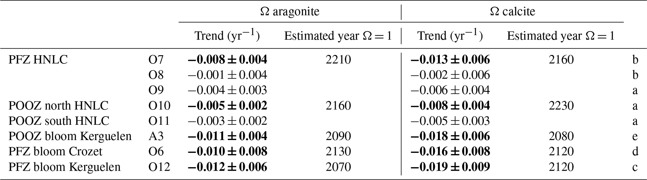
Table 5 Trends (per year) of Ω aragonite and Ω calcite, evaluated from the A_T and C_T dataset in the summer mixed layer at each station between (a) 1998 and 2019, (b) 1998 and 2017, (c) 1999 and 2019, (d) 2000 and 2019, and (e) 2005 and 2019. The significant trends (Student's t test) are represented in bold (at 95 %). Years of transition to Ω = 1 are also estimated when the trends are significant.

4.4 Saturation state of carbonate minerals

The accumulation of anthropogenic CO₂ in the ocean leads to acidification and decreases the saturation state of carbonate minerals in seawater (aragonite, Ω_Ar, and calcite, Ω_Ca). To date, surface waters are still super-saturated with respect to both aragonite and calcite (Ω > 1), but as Ω is minimum in the cold waters at high latitudes, the undersaturation state could be reached there by 2030–2050, depending on future CO₂ emission levels (Orr et al., 2005; McNeil and Matear, 2008), which raises particular concerns for calcifying species such as pteropods, planktonic foraminifera and coccolithophorids. As the year 2030 is approaching we should now see if these projections based on ocean biogeochemical models and different emission scenarios are real. Our observations clearly show a decrease in Ω_Ar and Ω_Ca over all of the study region (Table 5, Fig. S1). The lowest Ω values are found at the southernmost station (56.5^∘ S) and are around 1.5 for aragonite and 2.4 for calcite in January 2019. Note that according to the climatology by Takahashi et al. (2014), we expect lower values in September by about 0.2 to 0.3 for aragonite and 0.3 to 0.4 for calcite, indicating that undersaturation is not yet reached in surface waters in the southern Indian Ocean. The tipping point when the Southern Ocean will become saturated with respect to aragonite or calcite (Ω = 1) depends on the present value of Ω_Ar and Ω_Ca, their seasonality (Sasse et al., 2015), and their future trends.

To have a taste of when the tipping point might happen, we projected the trends of Ω_Ar and Ω_Ca estimated from our observations into the future. We estimated that undersaturation in January might not be reached before 2070 for aragonite and 2080 for calcite in regions where the pH trends are the fastest (Table 5, stations O12, A3 and O6). Based on the seasonal amplitude in Ω_Ar and Ω_Ca given by Takahashi et al. (2014), it might be reached in September between 15 and 25 years earlier. In the other regions it might not be reached within the next 100 years for aragonite in January (or within the next 40 years in September) and 150 years for calcite in January (100 years in September). Such calculations, however, remain highly uncertain as we have found large temporal variations in pH (hence Ω) trends, and we did not take into account CO₂ emission scenarios. In addition, the trends in Ω may not be uniform in the Southern Ocean. It can be noted that our fastest trends (−0.012 yr⁻¹ for aragonite and −0.019 yr⁻¹ for calcite; Table 5) correspond to the mean trends reported in the Drake Passage for summer (−0.013 yr⁻¹ for aragonite and −0.020 yr⁻¹ for calcite; Munro et al., 2015) or to the trend observed for aragonite in the eastern Indian sector over 1991–2000 (−0.018 yr⁻¹, whereas it was −0.007 yr⁻¹ over 2000–2011; Xue et al., 2018). Again, this highlights the sensitivity of the trends to the periods and regions and the need for more studies based on observations not only in surface waters but also in the water column to evaluate the rate of shoaling of Ω as previously shown in the eastern Indian southern sector (Pardo et al., 2017).

5 Concluding comments and perspectives

Given the importance of the Southern Ocean in climate (past, present and future) it is crucial to document and understand the changes occurring in this remote region. In this study, we investigated the evolution of CO₂ and pH in the surface layer of the Indian sector during summer using measurements of fCO₂, A_T and C_T obtained almost every year since 1998. This new analysis extends in time and for pH the previous work of Metzl (2009) and Lourantou and Metzl (2011), who estimated fCO₂ changes over 1991–2011 in the same region. It also extends their analyses using additional datasets (A_T–C_T) to quantify the drivers of the fCO₂ and pH trends including the contributions of C_ant evaluated here in subsurface waters. To our knowledge such a regular biogeochemical monitoring in the Southern Ocean is only conducted in the Drake Passage (since 2002; Munro et al., 2015). These time series are key to support the changes detected at the scale of the Southern Ocean or regional studies based on a limited number of reoccupations. A_T and C_T measurements are also essential as a complement to fCO₂ or pH as these are key properties, with temperature, that govern the variability in oceanic CO₂ sinks and sources and ocean acidification, but these data are still sparse in the Southern Ocean. In addition, there is a need to better evaluate models, not only from fCO₂ data or reconstructed fCO₂ products (Hauck et al., 2020) but also using C_T and A_T.

This study offers new fCO₂, C_T and A_T data at the surface and in the water column to validate GOBMs or ESMs (Kessler and Tjiputra, 2016) used to simulate the ocean CO₂ sink in the recent past or to predict the coupling between climate change and the ocean carbon cycle in the future. This would help to reduce the uncertainties and be confident in the projections of acidification in the Southern Ocean to better evaluate its impact on marine ecosystems, especially in marine protected areas such as around Crozet and Kerguelen islands (French Austral Lands and Seas nature reserves, UNESCO Heritage, https://whc.unesco.org/en/list/1603/, last access: 10 January 2022). Overall, this new analysis shows the importance of maintaining long-term observations. It is worth noting that the fCO₂ and pH trends were only evaluated for the summer season; complementing the ship observations with BGC-ARGO (Biogeochemical Argo) floats or drones such as at Drake Passage (Fay et al., 2018) and/or Saildrone USV (Sutton et al., 2021) is a challenge for the future studies at basin scale in the Southern Ocean in order to detect the trends in all seasons.

Appendix A: An evaluation of fCO₂ and pH trends in winter in the POOZ

In the Indian Ocean HNLC POOZ region, the modest CO₂ sink in summer is balanced by a CO₂ source in winter linked to upwelling and vertical mixing that bring C_T-rich deep waters to the surface (Metzl et al., 2006). When winter pCO₂ data were included in the air–sea CO₂ fluxes climatology (Takahashi et al., 2009), this led to an annual CO₂ source in the Indian POOZ of around +0.5 $\mathrm{mol}\mathrm{C}{\mathrm{m}}^{-\mathrm{2}}{\mathrm{yr}}^{-\mathrm{1}}$. The CO₂ source is stronger in the Indian sector of the POOZ due to higher winds and gas exchange coefficient in this region especially during winter (Takahashi et al., 2009; Wanninkhof and Triñanes, 2017). The stronger CO₂ source in the Indian POOZ is also confirmed by recent methods based on SOCAT fCO₂ observations (e.g. Chau et al., 2022), as well as when complementing the SOCAT fCO₂ data with GLODAP C_T data (Olsen et al., 2019) below the summer mixed layer to mimic the winter fCO₂ in surface waters (Mackay and Watson, 2021).

The winter CO₂ source south of the PF was also recently observed with autonomous probes on BGC-ARGO floats over 2014–2017 (SOCCOM project; Gray et al., 2018; Bushinsky et al., 2019), as well as in 2019 on a USV (Sutton et al., 2021). Interestingly, in June 2019, the USV sailed close to Station O11 and recorded high fCO₂ in the Indian POOZ at that period (maximum ΔfCO₂ of +25 µatm and mean ΔfCO₂ of +8.7 ± 7.4 µatm in this region). The fCO₂ recorded by the USV in June 2019 (mean fCO₂ = 398.7 ± 6.3 µatm) was much higher than our observations in January 2019 in the same region (fCO₂ = 376.4 ± 4.3 µatm). This is coherent with the fCO₂ seasonal cycle previously observed in this region (Metzl et al., 2006). There, the local hourly CO₂ source in June 2019 based on USV data was as high as +5 and +0.7 g C m⁻² per month when averaged in June–July 2019 in the Indian POOZ (Sutton et al., 2021). This is remarkably close to the climatological flux in June–July in the same region (+0.69 ± 0.62 g C m⁻² per month; Takahashi et al., 2009).

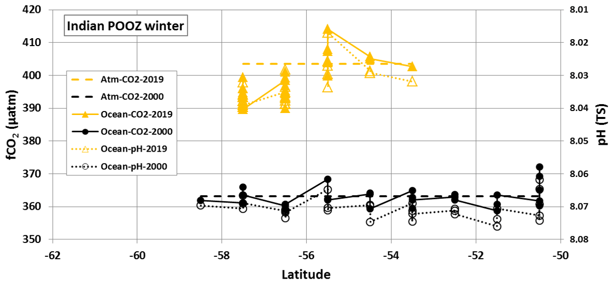
Figure A1 Monthly (gridded 1 × 1) fCO₂ and pH in the POOZ in austral winter 2000 (OISO-5, in black) and 2019 (USV, in yellow). Dotted lines represent the atmospheric fCO₂ in 2000 and 2019. The mean difference in fCO₂ is +35.8 µatm in 19 years, i.e. +1.9 µatm yr⁻¹. The mean difference in pH is −0.0368 in 19 years, i.e. −0.0019 yr⁻¹. Note that pH scale is reversed for easier reading.

Although there are very few fCO₂ observations in austral winter in this region, we attempted to use the winter data available in the Indian POOZ to compare with the trends we evaluated for summer. Here we used the data collected in August 2000 in the POOZ in the band 50–56^∘ S (Metzl et al., 2006) and compared them with the fCO₂ data from the USV in June 2019 in the same region (Sutton et al., 2021). Averaged monthly fCO₂ values were 362.9 (± 3.1) µatm in August 2000 and 398.7 (± 6.3) µatm in June 2019, indicating a clear fCO₂ increase of +35.8 µatm over 19 years (Fig. A1). This translates into a rate of +1.9 µatm yr⁻¹, which is close to that observed in the atmosphere (+2.1 µatm yr⁻¹ for 2000–2019) and in the range of the trend we deduced from our time series in summer 1998–2019 around Station O11 (+1.7 to +2.1 µatm yr⁻¹ depending on the datasets; Table 3). Below, we further investigate these data to evaluate whether the fCO₂ increase from winter 2000 to winter 2019 can also be mainly attributed to the accumulation of anthropogenic CO₂.

Based on the USV data (Sutton et al., 2021) available in SOCAT-v2021 (Bakker et al., 2021) we calculated the C_T concentrations from SST, fCO₂ and A_T (using a similar approach to that of Eq. 1); in June 2019 we estimated surface C_T concentrations between 2160 and 2185 µmol kg⁻¹ in the Indian POOZ from the USV data. This is higher than our observations in January 2019 (C_T = 2153.7 ± 0.6 µmol kg⁻¹ in the mixed layer at Station O11) and coherent with what we know about the C_T seasonality of around 15–20 µmol kg⁻¹ in this region (Metzl et al., 2006; Takahashi et al., 2014; Broullón et al., 2020; see also Fig. 3). At Station O11 in January 2019, the C_T concentration in the winter water (at 150 m) was 2175 µmol kg⁻¹. Correcting for organic matter remineralisation (AOU = 14 µmol kg⁻¹ at 150 m) the surface C_T concentration in winter would be 2164 µmol kg⁻¹. This is very close to the mean C_T deduced from the USV data (C_T = 2163.6 ± 5.0 µmol kg⁻¹) and, not surprisingly, higher than C_T concentrations calculated with fCO₂ data for August 2000 (C_T = 2151.4 ± 5.5 µmol kg⁻¹). The difference in C_T in winter over 19 years is +12.2 µmol kg⁻¹, leading to a trend of +0.64 µmol kg⁻¹ yr⁻¹ in the range of the decadal C_T trend we estimated in summer at Station O11 (+0.5 to +0.7 µmol kg⁻¹; Table 3) and close to the C_ant trend estimated below the mixed layer (+0.5 to +0.6 µmol kg⁻¹; Table 1). In addition, the pH calculated with fCO₂ data and A_T–S was 8.0706 (± 0.0032) in August 2000 and 8.0338 (± 0.0054) in June 2019 (Fig. A1), leading to a trend of −0.0019 yr⁻¹ in the same range as deduced from summer observations (Table 3). Although the derived trends for the winter season are only deduced from two periods (2019 versus 2000), these results support our conclusion based on repeated summer data that most of the fCO₂ and pH changes over 1998–2019 in the POOZ are driven by continuous anthropogenic carbon uptake (modulated by a small warming during summer).